The Magnetic Sun: Reversals and Long-Term Variations

Abstract

A didactic introduction to current thinking on some aspects of the solar dynamo is given for geophysicists and planetary scientists.

1 Introduction

For a long time, solar dynamo theory was in an advantageous situation compared to planetary dynamo theory. In the Sun, dynamo generated magnetic fields can be directly measured on the boundary of the turbulent, conducting domain where they are generated; and the timescales of their variations are short enough for direct observational follow-up. Solar observations also put many constraints on the motions in the convective zone, significantly restricting the otherwise very wide range of admissible mean field dynamo models.

In the past 15 years, however, planetary dynamo theorists have turned the table. Realistic numerical simulations of the complete geodynamo have been made possible by the rapid increase in the available computing power. While the parameter range for which such simulations are feasible is still far from realistic, extrapolations based on the available results have allowed important inferences on the behaviour of planetary dynamos (Christensen, Schmitt and Rempel 2009, Petrovay 2009).

In the light of these developments, learning from solar dynamo theory may have lost much of its former appeal to geophysicists, especially as it has become increasingly clear that the two classes of dynamos operate in fundamentally different modes, under very different conditions. Yet, keeping track with advance in the other field may not be without profit for either area. Even though the overall mechanisms may be very different, there may be many elements of each system where intriguing parallels exist.

A comprehensive review of solar dynamo theory is beyond the scope of the present article; for this, we refer the reader to papers by Petrovay (2000), Charbonneau (2005), Solanki, Inhester and Schüssler (2006) and Jones, Thompson and Tobias (2009).

Aside from reproducing the dipole dominance and other morphological traits of the geomagnetic field, two aspects of the geodynamo that are critical for judging the merits of its models are field reversals and long-term variations: whether or not a model can produce such effects in a way qualitatively, and if possible quantitatively similar to the geological record, has become a testbed for geodynamo simulations. It may thus be of special interest to review our current understanding of the analogues of these phenomena in the Sun. This is the purpose of the present paper.

In Section 2 we outline what solar observations suggest about the causes of reversals, i.e. the Babcock–Leighton mechanism. Two questions naturally arising from this discussion are given further attention in Sections 3 and 4. Section 5 briefly discusses some issues related to long-term variations of solar activity, while Section 6 concludes the paper, pointing out some interesting parallel phenomena in solar and planetary dynamos.

2 Reversals and global magnetism on the Sun

Information about large scale flows in the solar convective envelope can place important constraints on dynamo models. In the solar photosphere (the thin layer where most of the visible radiation originates) these flows can be directly detected by the tracking of individual features and by the Doppler effect. But in recent decades helioseismology (a technique analoguous to terrestrial seismology, see review by Howe 2009) has also shed light on subsurface flows. In particular, the internal differential rotation pattern is now known in much of the solar interior. It is characterized by a marked latitudinal differential rotation (faster equator, slower poles) throughout the convective envelope, while the radiative interior rotates like a rigid body. A thin transitional layer known as the tachocline separates the two regions. Meridional circulation, on the other hand is currently only known in the outermost part of the convective zone where it is directed from the equator towards the poles. A return flow is obviously expected in deeper layers but this has not yet been detected.

The invention of the magnetograph in 1959 marked a breakthrough in the study of solar magnetism. The output of this instrument, the magnetogram, is basically an intensity-coded map of the circular polarization over the solar disk. Circular polarization in turn is due to the Zeeman effect and, in a rather wide range (up to field strengths of $\sim 1\,$kG), it scales linearly with the line of sight component of the magnetic field strength. Apart from the saturation at kilogauss fields, then, a magnetogram is essentially a map of the line of sight magnetic field strength over the solar disk in the photosphere. Conventionally, fields with northern polarity are shown in white, while fields with southern polarity are shown in black.

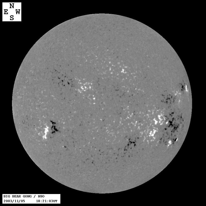
Figure 1: A solar magnetogram: a map of the line of sight magnetic field strength over the solar disk. Fields with northern (southern) polarity are shown in white (black). ©Big Bear Observatory

Figure 1 shows an arbitrarily chosen magnetogram as an example. It is immediately clear that the strongest magnetic concentrations, called active regions (AR), occur in bipolar pairs. Filtergrams and non-optical images showing the higher layers of the solar atmosphere confirm that these pairs mark the footpoints of large magnetic loops protruding from the Sun’s interior into its atmosphere. In white light images these active regions appear as dark sunspot groups and bright, filamentary facular areas. The lifetime of spots, faculæ and active regions is finite: turbulent motions in the solar photosphere ultimately lead to their dispersal over a period not exceeding a few weeks.

In addition to the strong active regions, Fig. 1 also displays some weaker and more extended magnetic concentrations, also in bipolar pairs (e.g. a bit upper left from the center). These features, only seen in magnetograms, are the remains of decayed active regions, the bipolar pair of flux concentrations being dispersed over an ever wider area of the solar surface. Ultimately, all that is left is a pair of unipolar areas —areas of quiet sun where the ubiquitous small-scale background magnetic field is dominated by one polarity or another.

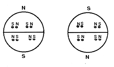
Figure 2: Sketch illustrating Hale’s polarity rules in the growing phase of two consecutive 11-year cycles (left and right, respectively)

We can see that the bipolar magnetic pairs are mostly oriented in the E-W direction, (with a slight tilt, to be discussed below). In the northern hemisphere, the N polarity patches lie to the west of their S polarity pairs, while in the southern hemisphere the situation is opposite. In the image, the direction of solar rotation is left to right and the rotational axis is approximately vertical and in the plane of the sky. “Western patches” are therefore referred to as the preceding polarity part of the active region, while their eastern pairs are the following polarity part. The rule we have just noticed then says that, at any given instant of time, preceding polarities of solar active regions are uniform over one hemisphere and opposite between the two hemispheres. Measurements performed during the course of several solar cycles show that, in any given hemisphere, the preceding polarity remains unchanged during the course of each 11-year solar cycle, while it alternates between cycles. This regularity, known as Hale’s polarity rules, is schematically illustrated in Fig. 2. This implies that the true period of solar activity is 22 years in the magnetic sense.

This sketch also shows one further regularity in the polarities. The weak large-scale magnetic field is usually opposite near the two rotational poles, and these polarities also alternate with a 22 year periodicity. However, the phase of this 22 year cycle is offset by about $\pi/2$ from the active region cycle, i.e. magnetic pole reversal does not occur in solar minimum. Instead, reversals typically take place 1–2 years after solar maximum, right in the middle of a cycle (as cycle profiles are asymmetric).

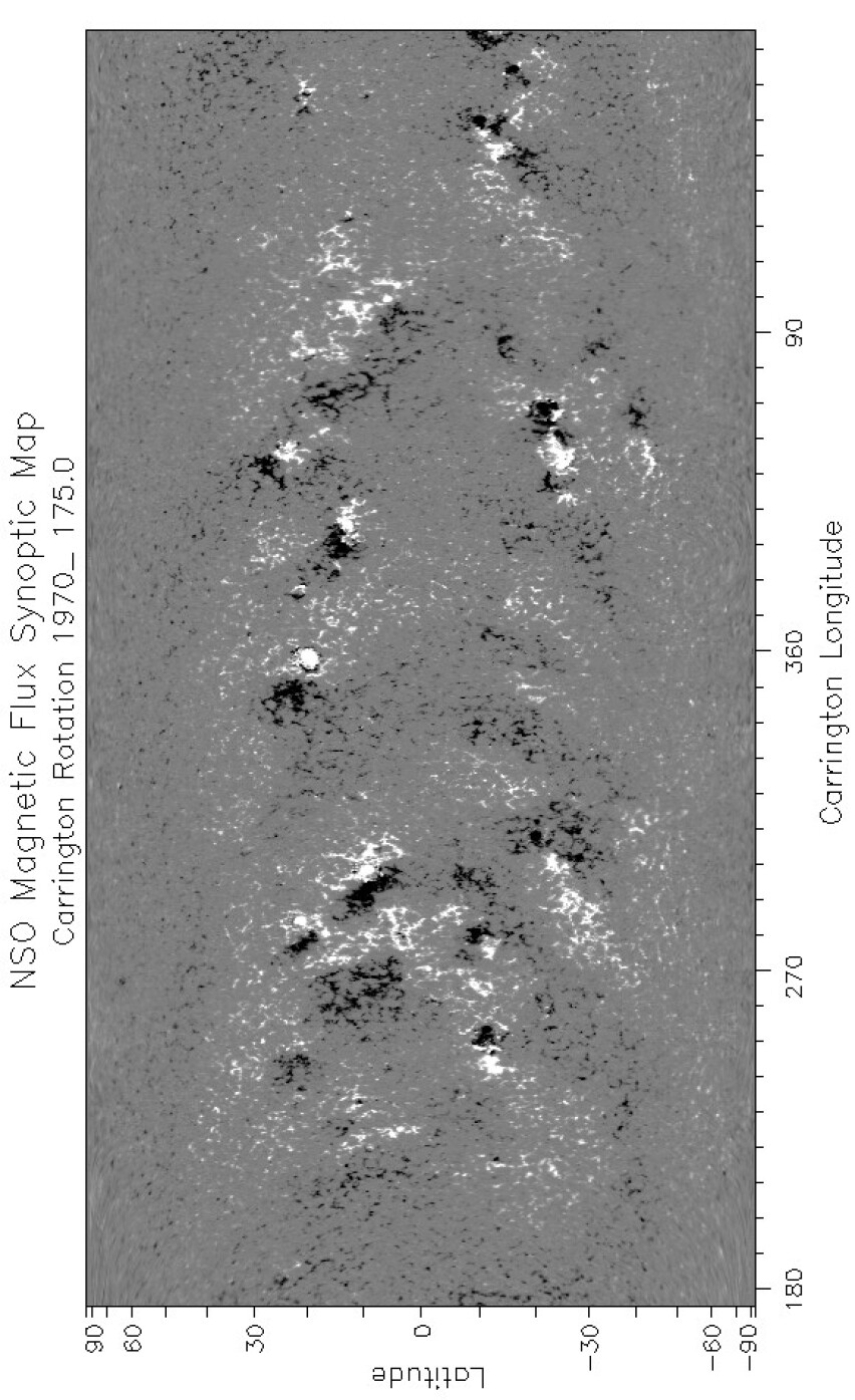
Figure 3: A synoptic magnetic map of the Sun ©NSO

Systematic magnetograph studies coupled with pioneering work on magnetic flux transport shed light on the apparent origin of the field reversal already in the 1960s (Babcock 1961, Leighton 1964). For a better understanding of how this so-called Babcock–Leighton mechanism works, consider a synoptic magnetic map like the one shown in Fig. 3. Such synoptic maps are essentially constructed by taking a narrow vertical strip from the center of each daily magnetogram (i.e. along the central meridian) and sticking them together from left to right, in a time sequence covering one synodic solar rotation. In this way we arrive at a “quasi-instantaneous” (in as much as $P_{\mathrm{rot}}\ll 11$ years) magnetic map of the full solar surface. In Fig. 3 we see further ample evidence of Hale’s polarity rules, but what is more interesting is the systematic deviation of the orientation of bipolar pairs from the E–W direction. It is clear that following polarity parts of active regions are systematically closer to the poles than their preceding polarity counterparts, and the tilt angle of the AR axis increases with heliographic latitude —a phenomenon known as Joy’s law.

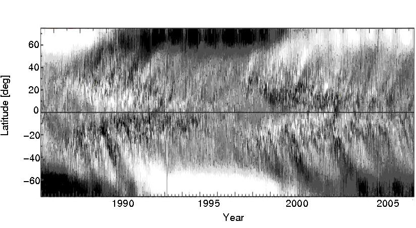
Figure 4: The magnetic butterfly diagram: longitudinally averaged magnetic field strength as a function of latitude and time, based on Mt. Wilson Observatory data. The grayscale goes from -2 G (black) to +2 G (white).

As a consequence of Joy’s law, upon the decay of active regions the resulting following polarity unipolar areas will be predominantly found on the poleward side of the active latitude belt. Now recall from Fig. 2 that in the early phase of a solar cycle, the following polarity in a given hemisphere is opposite to the polarity of the corresponding pole. As the decay of ever newer active regions replenishes its magnetic flux, this following polarity belt, located poleward of the active latitudes, will expand towards the pole, a process greatly helped by turbulent magnetic diffusion and by the advection of the large scale magnetic fields due to the Sun’s large scale meridional circulation. Ultimately, shortly after solar maximum, the preceding polarity patches around the two poles shrink to oblivion, and following polarity takes over: a reversal has taken place.

The process can be followed in the “magnetic butterfly diagram” shown in Fig. 4. Each pixel in this plot represents the intensity-coded value of the longitudinally averaged magnetic field strength at the given heliographic latitude and time. The butterfly wing shaped areas of intense magnetic activity at low latitudes represent the activity belts, migrating from medium latitudes towards the equator during the course of each solar cycle. The poleward drift apparent at high latitudes, in turn, corresponds to the poleward expansion of following polarity areas discussed above. It is clear that the reversal of the predominant magnetic polarity near the poles is due to this poleward drift, confirming the Babcock–Leighton scenario.

However compellingly the observations argue for such a scenario, two open questions remain.

1. What is the origin of the latitude-dependent tilt of active regions (Joy’s law)?
In the Babcock–Leighton scenario this tilt is clearly the ultimate cause of flux reversals. $\alpha\omega$ dynamo models rather naturally lead to predominantly toroidal, i.e. E–W oriented magnetic fields, so the tilt compared to this prevalent direction is likely to develop during the process of magnetic flux emergence from deeper layers into the atmosphere. This leads us to discuss flux emergence models in Section 3.

2. Do magnetic flux redistribution processes seen at the surface indeed play an important role in the dynamo, or are they just manifestations of similar, more robust processes taking place deep within the Sun?

The nice consistent cause-and-effect chain involved in the Babcock–Leighton scenario (AR tilt $+$ AR decay $\rightarrow$ $f$-polarity unipolar belt; $f$-polarity belt $+$ flux transport $\rightarrow$ reversal) seems to argue strongly for the first option. However, as we will see in Section 4 below, keeping the surface physically decoupled from the deeper layers is not easy, and such models invariably need to rely on some rather dubious physical assumptions. Thus, while parametric models of the first type can be fine-tuned to show impressive agreement with observations, their physical foundations remain shaky. Conversely, models based on more sound and plausible physical assumptions have had limited success in reproducing the details of observations. This constitutes the main dichotomy in current (mainstream) solar dynamo thinking, to be discussed in Section 4.

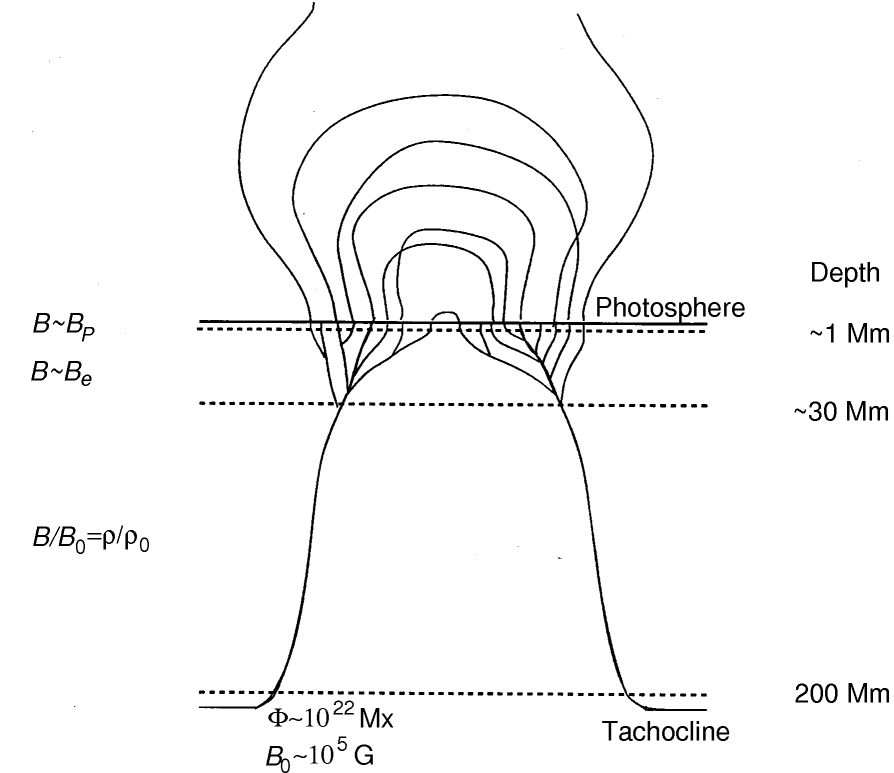
Figure 5: Sketch of the probable subsurface magnetic structure of an active region. $B_{P}=(2\mu_{0}P)^{1/2}$ is the pressure equipartition field strength, $P$ being the thermal gas pressure outside the flux tube. $B_{e}$ is the turbulent equipartition field strength as defined in the text.

3 Flux emergence

The current mainstream picture of the subsurface magnetic structure of solar active regions is sketched in Fig. 5. The observed distribution and proper motion patterns of sunspots and other magnetic elements in active regions are strongly suggestive of the so-called magnetic tree scenario: the cluster of smaller and larger magnetic flux tubes that manifest themselves as sunspots, facular points etc. in the photospheric layers of an active region are all connected in the deeper layers in a tree-like structure. The characteristic sizes of unipolar patches in a typical bipolar active region suggest that the trunk of this magnetic tree starts to fragment into branches at a relatively shallow depth, on the order of $\sim 10\,$% of the thickness of the convective zone. During the emergence of the tree structure, magnetic elements, corresponding to mesh points of the tree branches with the surface, naturally seem to converge into larger elements, ultimately forming large sunspots. This is just how sunspots are observed to be formed.

The natural initial configuration for such a magnetic loop, fragmented in its upper reaches, is a strong toroidal (i.e. horizontal and E–W oriented) magnetic flux bundle lying below the surface. The high field strength is a requirement imposed by the strict adherence to Hale’s polarity rules. Indeed, there are almost no exceptions to these rules among large active regions, so the drag force associated with the vigorous turbulent convective flows in the solar envelope must be small compared to other forces acting on the tube, in particular the curvature force. As the total magnetic flux of the tube must be similar to the flux of large active regions ($\sim 10^{22}\,$Mx), from this condition it can be estimated that the field strength must significantly exceed the equipartition field $B_{e}$ where the magnetic and turbulent pressures are equal ($B_{e}^{2}/2\mu_{o}=\rho\langle v^{2}\rangle/2$). It follows that $B\mathrel{\mathchoice{\vbox{\offinterlineskip\halign{\hfil$\displaystyle#$\hfil\cr>\cr\sim\cr}}}{\vbox{\offinterlineskip\halign{\hfil$\textstyle#$\hfil\cr>\cr\sim\cr}}}{\vbox{\offinterlineskip\halign{\hfil$\scriptstyle#$\hfil\cr>\cr\sim\cr}}}{\vbox{\offinterlineskip\halign{\hfil$\scriptscriptstyle#$\hfil\cr>\cr\sim\cr}}}}10^{4}\,$G ($\sim 1\,$T) in the deep convective zone.

It is however well known (Parker 1975) that such strong horizontal magnetic flux tubes cannot be stably stored in a superadiabatic or neutrally stable environment. The magnetic pressure implies that the gas pressure inside the flux tube is reduced in order to maintain pressure equilibrium with the environment. The associated decrease in density of the compressible plasma makes the flux tube magnetically buoyant. In order for such tubes to remain rooted in the solar interior while only a finite section of them emerges in the form of a loop, the initial tube must reside below the convective zone proper, in the subadiabatically stratified layer below. This layer coincides with the region of strong rotational shear between the rigidly rotating solar interior and the differentially rotating convective envelope, the above mentioned tachocline.

The emergence of flux loops formed on such strong toroidal flux bundles lying in the tachocline is driven by an instability. Often referred to as the Parker instability, this is a buoyancy driven instability of finite wavenumber perturbations of the tube (while the $k=0$ mode remains stable, so the tube remains rooted in the tachocline). The first models of this process employed the thin flux tube approximation (Spruit 1981) where the tube is essentially treated as a one-dimensional object. The emergence process was first followed into the nonlinear regime, throughout the convective zone, by Moreno-Insertis (1986); the action of Coriolis force and spherical geometry were incorporated in later models. Since the mid-1990s models have started to break away from the thin flux tube approximation and by now full 3D simulations of the emergence process have become the norm (see review by Fan 2004). Indeed, flux emergence models represent probably the most successful chapter in the research of the origin of solar activity in the last few decades.

As the total magnetic flux of the toroidal flux tube is set equal to typical active region fluxes, emergence models are left with only one free parameter: the initial field strength $B_{0}$. (Twist is introduced as a further free parameter in 3D models.) Comparing models with different values of $B_{0}$ to the observed structure and dynamics of sunspot groups, it was recognized about two decades ago (Petrovay 1991) that the value of $B_{0}$ must be surprisingly high, in the order of $10^{5}$ G, exceeding $B_{e}$ by an order of magnitude. This came as a surprise, as flux expulsion in a turbulent medium was known to concentrate diffuse magnetic fields in tubes and amplify them to $\sim B_{e}$, but not to significantly higher values. Yet there are at least four independent lines of argument to support this assertion.

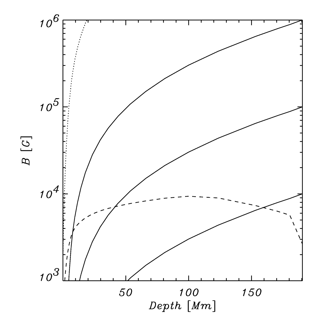
Figure 6: Magnetic field strength as a function of depth in the quasiadiabatic convective zone in an emerging flux tube for initial field strenghts of 10, 100, and 1000 kG (solid lines). Dashed line: turbulent equipartition field; dotted line: thermal equipartition field

1. Fragmentation depth. As the rise through the convective zone takes place on a relatively short timescale ($\sim 1\,$month), matter inside the flux tube expands adiabatically. Most of the convective zone (except the uppermost few hundred km) is also very nearly adiabatically stratified, and the magnetic pressure is negligible compared to the thermal pressure here, so the relative density contrast between the inside of the tube and its surroundings will remain relatively small. The field strength inside the loop is then given by $B/B_{0}=\rho/\rho_{0}$, the ’0’ index referring to values at the bottom of the convective zone. The resulting values of $B$ as a function of depth $z$ are plotted in Fig. 6. It is apparent that at a certain depth $B$ drops below the turbulent equipartition field strength $B_{e}$. Above this level the magnetic field is unable to suppress turbulence and the external turbulent motions will penetrate the tube. Flux expulsion processes taking place in parallel with the further emergence of the loop are then expected to fragment the top of the loop into a number of smaller flux tubes, resulting in the magnetic tree structure. As we have seen, observations suggest that this fragmentation occurs at a depth of a few tens of megameters: Fig. 6 then clearly suggests $B_{0}\sim 10^{5}\,$G.
   

2. Emergence latitudes. For weaker tubes, the buoyancy and the curvature force are also weaker, so the Coriolis force, independent of the field strength, will play a more dominant role in the dynamics of the emerging loop. Tubes with $B_{0}\ll 10^{5}\,$G are so strongly deflected by the Coriolis force that they will emerge approximately parallel to the rotation axis. As the bottom of the convective zone lies at 0.7 photospheric radii, weak flux tubes emerging from here cannot reach the surface at latitudes below 45 degrees, in contradiction to observations (Choudhuri and Gilman 1987, Choudhuri 1989).
   

3. Joy’s law. Tubes with higher values of $B_{0}$ will emerge approximately radially, yet the effect of Coriolis force on them is not negligible. The meridional component of the Coriolis force acting on the downflows in the tilted legs of the emerging loop will twist the plane of the loop out of the azimuthal plane, resulting in a tilt in the orientation of active regions relative to the E–W direction. This tilt increases with heliographic latitude, thus explaining the observed Joy’s law. Quantitative comparison between models and observations again shows that Joy’s law is best reproduced for $B_{0}\sim 10^{5}\,$G (D’Silva and Choudhuri 1993).
   

   

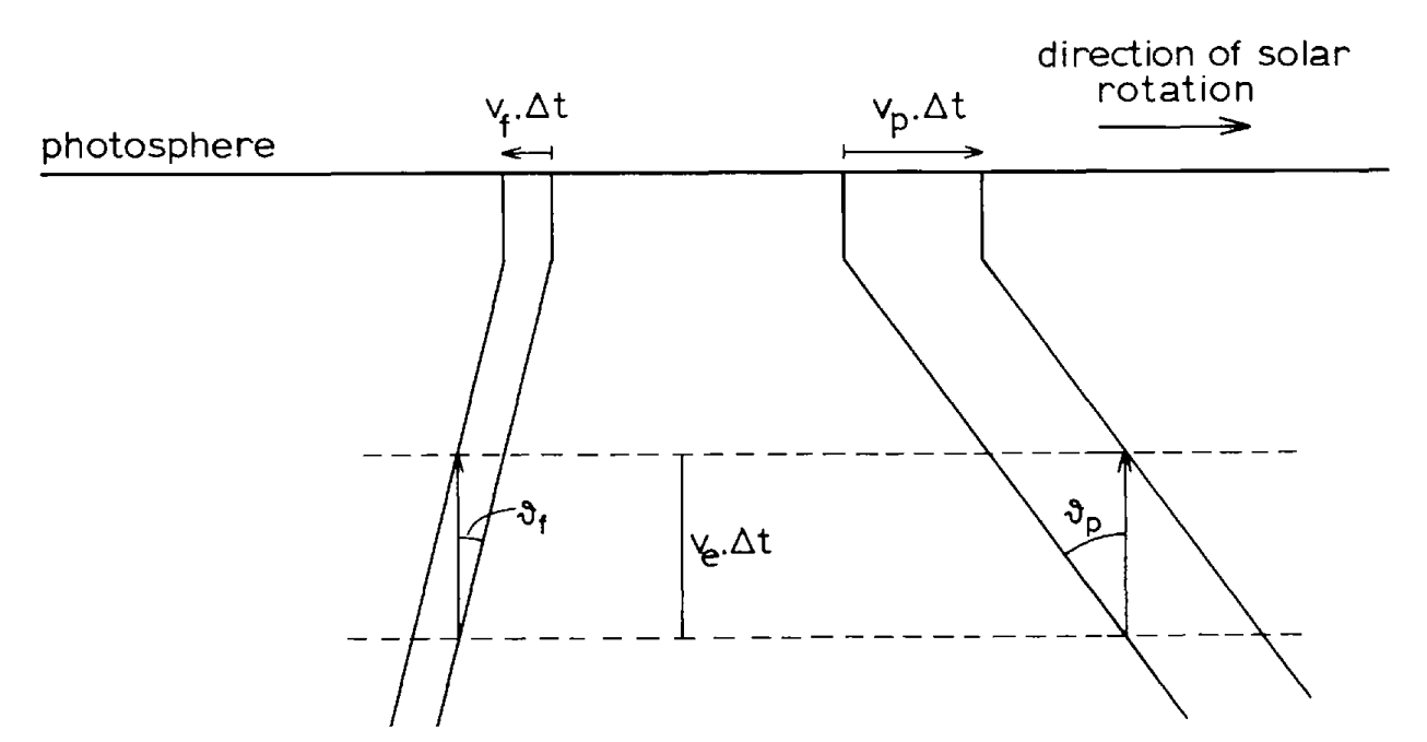
   Figure 7: Interpretation of sunspot proper motions by the emergence of an asymmetric flux loop (after van Driel-Gesztelyi and Petrovay 1990)

4. Sunspot proper motions. The azimuthal component of the Coriolis force acting on the downflows in the tilted legs of the emerging loop has two consequences. On the one hand, as this component is westward in both legs, it will distort the shape of the emerging loop so that it will become asymmetrical, the following leg being less inclined to the vertical than the preceding leg. On the other hand, this westward force results in a wavelike translational motion of the loop as a whole compared to the ambient medium: the active region is then expected to rotate faster than quiet sun plasma. It is indeed well known that sunspots and other magnetic tracers generally show some superrotation compared to the Doppler rotation rate of the ambient plasma. In the past, some confusion arose due to the fact that this superrotation appears to be time dependent: newborn sunspot groups rotate fastest, their rotation rate steadily declines during the growth phase of the group, until it becomes stagnant at a rate only slightly above the plasma rotation rate from the time when the group reaches its maximal development. This apparent change in the rotation rate, however, was shown to be a purely geometrical projection effect (van Driel-Gesztelyi and Petrovay 1990), as a consequence of the asymmetrical shape of the loop (cf. Fig. 7). Again, detailed quantitative comparisons of sunspot proper motion observations with the dynamics of emerging flux tube models (Moreno-Insertis, Caligari and Schuessler 1994, Caligari, Moreno-Insertis and Schüssler 1995) indicate optimal agreement for $B_{0}\sim 10^{5}\,$G.

In summary: flux emergence models have led to the rather firm conclusion that solar active regions are the product of the buoyancy driven rise of strong magnetic flux loops through the convective zone. The loops arise from small perturbations of strong toroidal flux bundles lying in the solar tachocline, at the bottom of the convective zone. (These tubes may be preexistent, or alternatively they may detach from a continuous flux distribution as a result of the perturbation.) A number of independent arguments indicate that the field strength in these toroidal tubes is on the order of $10^{5}\,$G. The origin of the tilt in active regions orientations relative to the E–W direction is clearly identified as the action of Coriolis force on the emerging flux loops, twisting them out of the azimuthal plane.

4 Alternative global scenarios for the solar dynamo

As we have seen in Sections 2 and 3, the Babcock–Leighton mechanism offers a very attractive explanation of the cyclic polar reversals and activity variations observed on the Sun. During the flux emergence process, the Coriolis force twists the plane of the flux loops out of the azimuthal plane, so they acquire a poloidal magnetic field component. With the turbulent dispersal of the active regions, this poloidal field component contributes to the large-scale diffuse solar magnetic field. Advected towards the poles by meridional circulation, it ultimately brings about the reversal of the global poloidal magnetic field of the Sun. This reversed poloidal field is then advected down into the tachocline by the meridional circulation near the poles. Continuity requires that plasma advected to the poles near the surface by meridional circulation must be returned to the equator at some depth; in the simplest case of a one-cell circulation this will occur near the bottom of the convective zone. This deep equatorward counterflow then advects the poloidal field towards the equator at some slower speed, while differential rotation winds it up, resulting in an ever stronger toroidal field component. By the time it reaches latitudes below about $35^{\circ}$, this advected toroidal field reaches, at least intermittently, the intensity of $\sim 10^{5}\,$G and starts to erupt in the form of buoyancy driven loops, closing the cycle. The equatorward propagation of active latitudes, manifest in the butterfly diagram, is thus solely due to the advection of toroidal fields by the meridional circulation.

Flux transport dynamos:

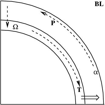
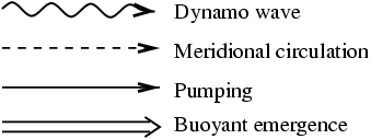
Interface dynamos:

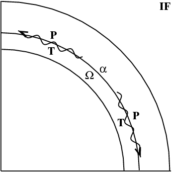
Figure 8: Sketches illustrating the basic concepts of the two main solar dynamo scenarios

This scenario was already qualitatively outlined by Babcock (1961) (with the difference that he attributed the rise and tilt of flux loops to helical convection). By now we have detailed quantitative models for the solar dynamo along these lines (Dikpati and Charbonneau 1999, Nandy and Choudhuri 2001). As all migration phenomena in the butterfly diagram are explained by the advection of magnetic flux in this picture, these models are known as flux transport dynamos.

Flux transport models have become quite successful in reproducing many of the observational details such as the shape of the butterfly diagram. This is to a large extent due to their very good parametrizability. There are, however, serious doubts concerning their physical consistency.

One issue concerns vertical flux transport. In order to have a poleward flux transport near the surface and an equatorward transport near the bottom, the surface and the tachocline must be kept incomunicado on a timescale comparable to the solar cycle. However, simple mixing length estimates suggest that the turbulent magnetic diffusivity in the convective zone is in the range $10^{2}$–$10^{3}\,$km²/s, so the timescale for the surface field to diffuse down to the bottom across the the convective zone of depth $d=2\cdot 10^{5}\,$km is a few years, certainly less than the solar cycle length. The above mentioned value of the diffusivity is confirmed by calibrations based on surface flux redistribution. So, in order to effectively decouple surface and bottom, flux transport dynamos invariably need to rely to some ad hoc assumptions regarding magnetic diffusivity: suppressing it in the bulk of the convective zone, making it highly anisotropic etc.

A further difficulty is related to the flow pattern envisaged in these kinematic models. The equatorward return flow of meridional circulation is assumed to spatially overlap with the tachocline, i.e. the subadiabatic layer where the toroidal field can be stably stored and where it is amplified by the strong rotational shear. But this assumption is very dubious from a dynamical/thermal point of view. To penetrate the subadiabatically stratified upper radiative zone, the plasma partaking in the meridional flow would have to get rid of its extra entropy so buoyancy will not inhibit its submergence. This, however, can only occur on a slow, thermal timescale. Numerical estimates show that the maximal circulation speed in the subadiabatic tachocline is a few cm/s, way too slow for flux transport models to work.

An alternative approach to the solar dynamo is, then, to try to construct models from first principles, without introducing physically unsubstantiated assumptions. Such a model cannot ignore the achievements of flux emergence models and needs to be based on the assumption that the strong toroidal flux tubes responsible for solar activity phenomena reside in the subadiabatic tachocline, and then are presumably also generated there, given the strong rotational shear.

Significant work has been done on the role of a stably stratified convective overshoot layer, coincident witha shear layer (tachocline) in large-scale dynamos (cf. Tobias 2009 and Brandenburg 2009). The slow meridional circulation allowed here cannot be responsible for the latitudinal migration of the toroidal field as seen in the butterfly diagram. Instead, this must be the manifestation of a classic dynamo wave, as already suggested by Parker (1955). The tachocline is, however, probably not turbulent enough to support a strong $\alpha$-effect, so the site of the $\alpha$-effect must be in the convective zone, adjacent to the tachocline, where convective downflows diverge, resulting in $\alpha<0$ in the northern hemisphere as required for an equatorward propagating dynamo wave at the low latitudes where $\partial\Omega/\partial r>0$.

In these interface dynamos, then, the dynamo wave is excited as a surface wave on the interface between the tachocline and the convective zone. Their classic analytical prototype was constructed by Parker (1993). At higher latitudes, where $\partial\Omega/\partial r<0$ this model naturally results in a poleward propagating dynamo wave, possibly explaining the poleward migration of unipolar areas and other phenomena in this part of the Sun. This is an attractive feature of these models, but the question naturally arises, whether the equatorward return flow that must be present in the lower convective zone if not in the tachocline, i.e. on one side of the interface will affect these results. This was examined by Petrovay and Kerekes (2004) in an extension of Parker’s analytical work to the case of a meridional flow. It was found that for parameters relevant to the solar case the meridional flow is unable to overturn the direction of propagation of dynamo waves, nor will it significantly affect their growth rates. For a related study of the effect of other flux transport mechanisms on the interface dynamos see Mason, Hughes and Tobias (2008).

A number of detailed numerical interface dynamos models have been constructed for the Sun (Charbonneau and MacGregor 1997, Markiel and Thomas 1999, Dikpati, Gilman and MacGregor 2005). It must be admitted that at present they are unable to reproduce the observed features of the solar activity cycle as satisfactorily as some flux transport models can. However, this is clearly a consequence of the fact that these models lack the kind of physical arbitrariness that characterizes some flux kinematical transport models, where the arbitrary prescription of flow geometries and amplitudes (esp. for the meridional flow) leaves much more space to play around with parameters until an acceptable fit to observations results.

5 Long term variations

In the geodynamo, field reversals and long-term variations are closely related. Indeed, reversals are the most important kind of long term variation. In the Sun, however, the field regularly reverses in every 11-year cycle: in fact, reversals are the essence of the 11/22-year cycle. Long term variations, in turn, are a completely independent topic. It is impossible to give a comprehensive review of this area in the present introductory paper (see Usoskin and Mursula 2003, Usoskin 2008 for much more exhaustive overviews); instead, we limit ourselves to mentioning some salient points and recent results.

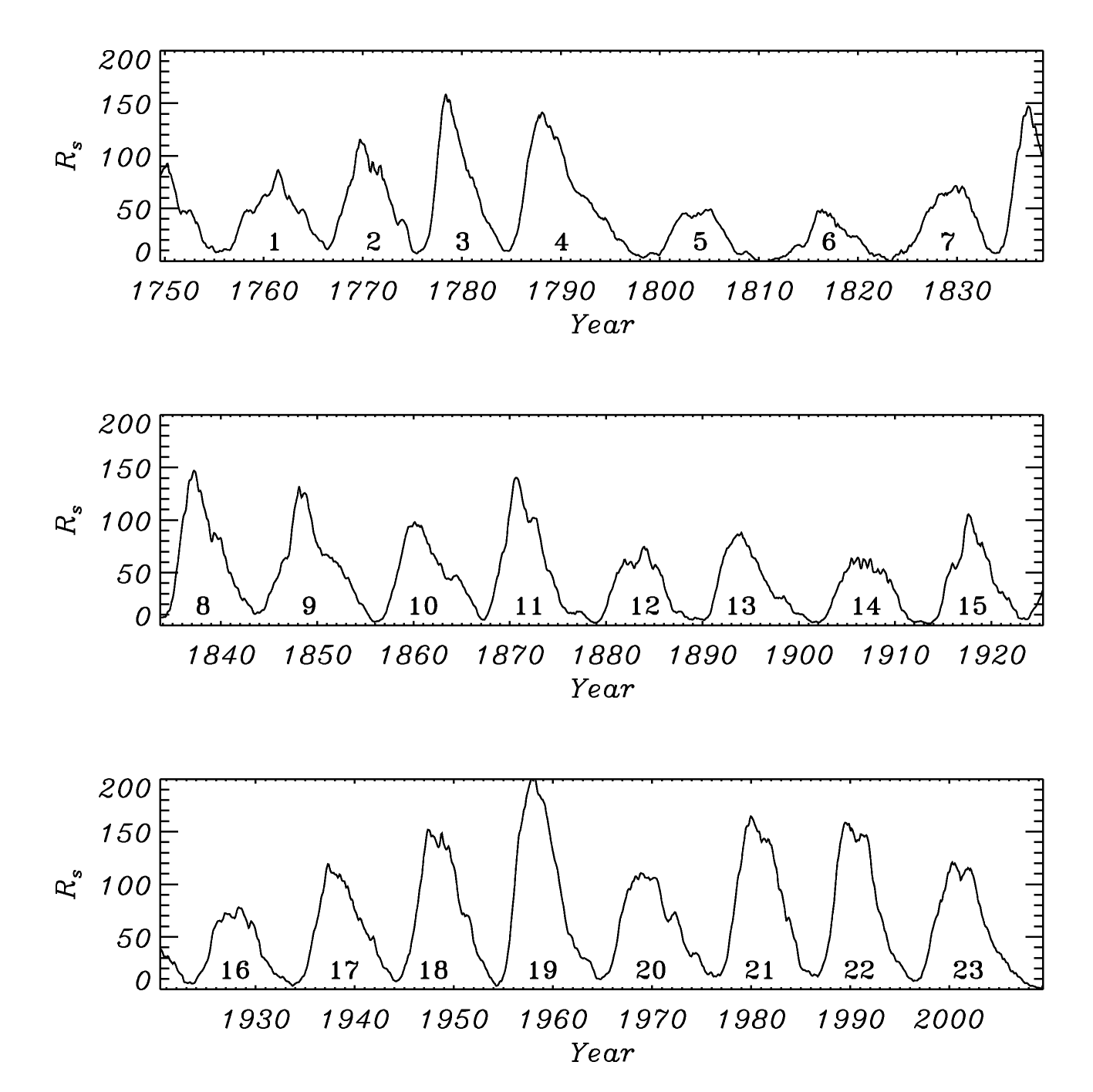
Figure 9: Variation of the smoothed (13-month boxcar average) relative sunspot number with time. Solar cycles are numbered.

Figure 9 presents the variation of the relative sunspot number in the last three centuries, for which the most reliable direct data exist. From historical solar observations going back another century we know that immediately before the period covered by Fig. 9, the Sun underwent an unusally quiet period lasting nearly 70 years: in this so-called Maunder minimum there were hardly any spots seen on the Sun at all. At the other extreme lies the Modern Maximum: the series of unusually strong cycles that started in the mid-20th century and seems to be just about to come to an end now.

Various terrestrial proxies of solar activity have made it possible to reconstruct long term activity variations (albeit not necessarily individual cycles) over a substantially longer time span. The best results were found from studies of the abundance of the cosmogenic ¹⁰Be isotope in Greenland ice cores. These studies led to a reconstruction of the history of solar activity in the last 9000 years with a time resolution of about 10 years (Beer, Vonmoos and Muscheler 2006). Recently, data with even better, annual resolution have become available for the last six centuries (Berggren et al. 2009).

One interesting result from these studies concerns the histogram of decadal activity levels (Usoskin, Solanki and Kovaltsov 2007). It was found that the overall shape of this histogram is compatible with a normal distribution; however, significant excesses or “shoulders” appear at both extremes. In other words, times of very low and very high solar activity are overabundant relative to a Gaussian statistics. These results suggest that grand minima and grand maxima are more than random fluctuations: they are indeed physically distinct states of the dynamo. Long term variations in the intermediate states, in turn, seem to be driven by stochastic effects, resulting in nearly Gaussian statistics.

Attempts to explain the long term variation in solar activity, as well as grand minima and maxima, include stochastic fluctuations in dynamo parameters (Ossendrijver 2000, Moss et al. 2008); nonlinear dynamos with chaotic behaviour (Beer, Tobias and Weiss 1998, Brooke et al. 1998) or with two alternative stationary dynamo solutions (Petrovay 2007). The shape of the histogram discussed above suggests a bimodal solution with strong stochastic forcing resulting in an actual solution that random walks in between the attractors for most of the time.

It should be noted that radionuclide based reconstructions of solar activity involve several uncertainties. On the long timescales we are concerned with, the most important such effect is the parallel long term variation in the geomagnetic field. The atmospheric cosmic ray flux, and thereby the radionuclide production rate, is the net result of the shading effects of both the interplanetary and the terrestrial magnetic fields, so long-term normalization of the solar modulation crucially depends on the correct subtraction of the geomagnetic contribution. Issues such as just how exceptionally strong the most recent grand maximum (the Modern Maximum) was, are strongly influenced by these effects.

6 Conclusion: analogies and differences with respect to the geodynamo

At the most basic level, the same processes generate magnetic field in the Earth’s core and inside the Sun: the shearing of magnetic field lines by differential rotation ($\Omega$-effect) and their twisting by helical motions ($\alpha$-effect) that obtain a preferred handedness from the action of Coriolis forces. Also, some magnetic phenomena may have similar causes. For example, paired flux spots at low latitudes in the geomagnetic field at the core-mantle boundary have been tentatively explained by the expulsion of toroidal flux tubes (Bloxham 1986), in analogy to the generation of sunspots. But although this interpretation is supported by some geodynamo models (Christensen and Olson 2003), other explanations for low-latitude magnetic structures have been put forward (Finlay and Jackson 2003). Meridional flow is thought to play the essential role for reversals of the solar magnetic field. This has also been demonstrated in a simple reversing geodynamo model (Wicht and Olson 2004). However, the reversal behaviour in this model is nearly cyclic as in case of the Sun, in contrast to the stochastic reversals of the geomagnetic field. In a less idealized geodynamo model with random reversals, impulsive upwellings have been identified as the cause for polarity changes (Aubert, Aurnou and Wicht 2008). These upwellings transport and amplify a multipolar magnetic field from depth to the outer boundary. While possible analogies between the solar dynamo and the geodynamo can stimulate our thinking, we must keep their limitations in mind.

Which differences in physical conditions lead to the rather distinct behaviour of the solar dynamo and the geodynamo? One important difference is that the plasma in the solar convection zone is sufficiently compressible and that the field strength is high enough so that magnetic pressure and magnetic buoyancy play an essential role for the dynamics of flux tubes. These effects are probably unimportant in Earth’s core. Another difference is that the Coriolis force has a stronger influence in the geodynamo than it has in the slowly rotating Sun. This notion is supported by the observation that much more rapidly rotating stars of low mass seem to have strong large-scale magnetic fields that are frequently dominated by the axial dipole component (Donati et al. 2008). Their observed field strengths follow the same scaling law as the observed fields of Earth and Jupiter and the field intensity found in geodynamo models at sufficiently rapid rotation (Christensen, Holzwarth and Reiners 2009). A third difference arises from the much slower motion and therefore lower magnetic Reynolds number in the geodynamo.

The moderate value of the magnetic Reynolds number makes the magnetic induction process in the Earth’s core amenable to direct numerical simulations without the need to take recourse to turbulent magnetic diffusivities or parameterized turbulent $\alpha$-effects. This is perhaps the most important reason for the success of geodynamo models in reproducing many observed properties of the geomagnetic field without need for ad-hoc assumptions. However, our more limited knowledge of the geomagnetic field at the top of the core, in comparison to that of the field in the solar photosphere, makes the task simpler for a geodynamo modeller. Also, helioseismology has revealed the distribution of zonal flow in the solar convection zone and a fully consistent solar dynamo model must reproduce this flow pattern as well as the magnetic field properties. Comparable information is lacking for the Earth and a geodynamo model can be declared successful once it captures the general properties of the large-scale geomagnetic field.