Estimates of MM type for the multivariate linear model

Nadia L. Kudraszowaa{}^{\text{a}} and Ricardo A. Maronnabb{}^{\text{b}}
aa{}^{\text{a}}University of La Plata and CONICET (nkudraszow@mate.unlp.edu.ar)
bb{}^{\text{b}}University of La Plata and C.I.C.P.B.A. (rmaronna@retina.ar)
Abstract

We propose a class of robust estimates for multivariate linear models. Based on the approach of MM estimation (Yohai 1987, [27]), we estimate the regression coefficients and the covariance matrix of the errors simultaneously. These estimates have both high breakdown point and high asymptotic efficiency under Gaussian errors. We prove consistency and asymptotic normality assuming errors with an elliptical distribution. We describe an iterative algorithm for the numerical calculation of these estimates. The advantages of the proposed estimates over their competitors are demonstrated through both simulated and real data.

Keywords: Robust methods; MM-estimate; Multivariate linear model.

1 Introduction

Consider a multivariate linear model (MLM) with random predictors, i.e., we observe n๐‘›n independent identically distributed (i.i.d.) (p+q)๐‘๐‘ž(p+q)-dimensional vectors, ๐ณi=(๐ฒiโ€ฒ,๐ฑiโ€ฒ)subscript๐ณ๐‘–superscriptsubscript๐ฒ๐‘–โ€ฒsuperscriptsubscript๐ฑ๐‘–โ€ฒ\mathbf{z}_{i}=(\mathbf{y}_{i}^{\prime},\mathbf{x}_{i}^{\prime}) with 1โ‰คiโ‰คn1๐‘–๐‘›1\leq i\leq n, where ๐ฒi=(yiโ€‹1,โ€ฆ,yiโ€‹q)โ€ฒโˆˆโ„q,๐ฑi=(xiโ€‹1,โ€ฆ,xiโ€‹p)โ€ฒโˆˆโ„pformulae-sequencesubscript๐ฒ๐‘–superscriptsubscript๐‘ฆ๐‘–1โ€ฆsubscript๐‘ฆ๐‘–๐‘žโ€ฒsuperscriptโ„๐‘žsubscript๐ฑ๐‘–superscriptsubscript๐‘ฅ๐‘–1โ€ฆsubscript๐‘ฅ๐‘–๐‘โ€ฒsuperscriptโ„๐‘\mathbf{y}_{i}=(y_{i1},\ldots,y_{iq})^{\prime}\in\mathbb{R}^{q},\;\;\;\mathbf{x}_{i}=(x_{i1},\ldots,x_{ip})^{\prime}\in\mathbb{R}^{p} and โ€ฒ denotes the transpose. The ๐ฒisubscript๐ฒ๐‘–\mathbf{y}_{i} are the response vectors and the ๐ฑisubscript๐ฑ๐‘–\mathbf{x}_{i} are the predictors and both satisfy the equation

๐ฒi=๐0โ€ฒโ€‹๐ฑi+๐ฎiโ€‹โ€„โ€„โ€„โ€„โ€„โ€„1โ‰คiโ‰คn,subscript๐ฒ๐‘–superscriptsubscript๐0โ€ฒsubscript๐ฑ๐‘–subscript๐ฎ๐‘–1๐‘–๐‘›\mathbf{y}_{i}=\mathbf{B}_{0}^{\prime}\mathbf{x}_{i}+\mathbf{u}_{i}\;\;\;\;\;\;1\leq i\leq n, (1.1)

where ๐0โˆˆโ„pร—qsubscript๐0superscriptโ„๐‘๐‘ž\mathbf{B}_{0}\in\mathbb{R}^{p\times q} is the matrix of the regression parameters and ๐ฎisubscript๐ฎ๐‘–\mathbf{u}_{i} is a q๐‘žq-dimensional vector independent of ๐ฑisubscript๐ฑ๐‘–\mathbf{x}_{i}. If ๐ฑiโ€‹p=1subscript๐ฑ๐‘–๐‘1\mathbf{x}_{ip}=1 for all 1โ‰คiโ‰คn1๐‘–๐‘›1\leq i\leq n, we obtain a regression model with intercept.

We denote the distributions of ๐ฑisubscript๐ฑ๐‘–\mathbf{x}_{i} and ๐ฎisubscript๐ฎ๐‘–\mathbf{u}_{i} by G0subscript๐บ0G_{0} and F0subscript๐น0F_{0}, respectively, and ๐šบ0subscript๐šบ0\mathbf{\Sigma}_{0} is the covariance matrix of the ๐ฎisubscript๐ฎ๐‘–\mathbf{u}_{i}. The p๐‘p-multivariate normal distribution with mean vector ๐๐\boldsymbol{\mu} and covariance matrix ๐šบ๐šบ\mathbf{\Sigma} is denoted by Npโ€‹(๐,๐šบ)subscript๐‘๐‘๐๐šบN_{p}(\boldsymbol{\mu},\mathbf{\Sigma}).

In the case of ๐ฎisubscript๐ฎ๐‘–\mathbf{u}_{i} with distribution Nqโ€‹(๐ŸŽ,๐šบ0)subscript๐‘๐‘ž0subscript๐šบ0N_{q}(\mathbf{0},\mathbf{\Sigma}_{0}), the maximum likelihood estimate (MLE) of ๐0subscript๐0\mathbf{B}_{0} is the least squares estimate (LSE), and the MLE of ๐šบ0subscript๐šบ0\mathbf{\Sigma}_{0} is the sample covariance matrix of the residuals. It is known that these estimates are not robust: a small fraction of outliers may have a large effect on their values.

Several approaches have been proposed to deal with this problem. The first proposal of a robust estimate for the MLM was given Koenker and Portnoy [14]. They proposed to apply a regression M-estimator, based on a convex loss function, to each coordinate of the response vector. The problems with this estimate is lack of affine equivariance and zero breakdown point. Several other estimates without these problem were defined later. Rousseeuw et al. [22] proposed estimates for the MLM based on a robust estimate of the covariance matrix of ๐ณ=(๐ฑโ€ฒ,๐ฒโ€ฒ)๐ณsuperscript๐ฑโ€ฒsuperscript๐ฒโ€ฒ\mathbf{z}=(\mathbf{x}^{\prime},\mathbf{y}^{\prime}). Bilodeau and Duchesne [5] extended the S-estimates introduced by Davies [7] for multivariate location and scatter; then Van Aelst and Willems [26] studied the robustness of these estimators. Agullรณ et al. [1] extended the minimum covariance determinant estimate introduced by Rousseeuw [21] and Roelandt et al. [20] extended the definition of GS-estimates introduced by Croux et al. [6]. These estimates have a high breakdown point but are not highly efficient when the errors are Gaussian and q๐‘žq is small. In order to solve this, Agullรณ et al. [1] improved the efficiency of their estimates, maintaining their high breakdown point, by considering one-step reweighting and one-step Newton-Raphson GM-estimates. Garcรญa Ben et al. [8] extended ฯ„๐œ\tau-estimates for multivariate regression, obtaining a estimate with high breakdown point and a high Gaussian efficiency. Another important approach to obtain robust and efficient estimates is contrained M (CM) estimation, proposed by Mendes and Tyler [17] for regression and by Kent and Tyler [13] for multivariate location and scatter. The bias of CM estimates for regression was studied by Berrendero et al. [3]. Following this approach, Bai et al. [2] proposed CM estimates for the multivariate linear model.

In this paper we propose robust estimates for the linear model based on the MM approach, first proposed by Yohai [27] for the univariate linear model, and later by Lopuhaรค [15], Tatsuoka et al. [25] and Salibiรกn-Barrera et al. [23] for multivariate location and scatter. We show that our estimates have both a high breakdown point and a high normal efficiency.

In Section 2 we define MM-estimates for the MLM and prove some properties. In Section 3 and 4 we study their breakdown point and Influence Function. In Section 5 and 6 we study the asymptotic properties (consistency and asymptotic normality) of the MM-estimates assuming random predictors and errors with an elliptical unimodal distribution. In Section 7 we describe a computing algorithm based on an iterative weighted MLE. In Section 8 we present the results of a simulation study and a real example in Section 9. All the proofs can be found in the Appendix.

2 Definition and properties

Before defining our class of robust estimates for the MLM, we will define a robust estimate of scale.

Definition 1.

Given a sample of size n๐‘›n, ๐ฏ=(v1,โ€ฆ,vn)๐ฏsubscript๐‘ฃ1โ€ฆsubscript๐‘ฃ๐‘›\mathbf{v}=(v_{1},\ldots,v_{n}), an M-estimate of scale sโ€‹(๐ฏ)๐‘ ๐ฏs(\mathbf{v}) is defined as the value of s๐‘ s that is solution of

1nโ€‹โˆ‘i=1nฯ0โ€‹(vis)=b,1๐‘›superscriptsubscript๐‘–1๐‘›subscript๐œŒ0subscript๐‘ฃ๐‘–๐‘ ๐‘\displaystyle{\frac{1}{n}\displaystyle{\sum_{i=1}^{n}\rho_{0}\left(\frac{v_{i}}{s}\right)}=b,} (2.1)

where bโˆˆ(0,1)๐‘01b\in(0,1), or s=0๐‘ 0s=0 if โ™ฏโ€‹(vi=0)โ‰ฅnโ€‹(1โˆ’b)โ™ฏsubscript๐‘ฃ๐‘–0๐‘›1๐‘\sharp(v_{i}=0)\geq n(1-b), where โ™ฏโ™ฏ\sharp is the symbol for cardinality.

In this paper we use b=0.5๐‘0.5b=0.5, which ensures the maximal asymptotic breakdown point (see [11]).

The function ฯ0subscript๐œŒ0\rho_{0} should satisfy the following definition.

Definition 2.

A ฯ๐œŒ\rho-function will denote a function ฯโ€‹(u)๐œŒ๐‘ข\rho(u) which is a continuous nondecreasing function of |u|๐‘ข|u| such that ฯโ€‹(0)=0๐œŒ00\rho(0)=0, supuฯโ€‹(u)=1subscriptsupremum๐‘ข๐œŒ๐‘ข1\sup_{u}\rho(u)=1, and ฯโ€‹(u)๐œŒ๐‘ข\rho(u) is increasing for nonnegative u๐‘ขu such that ฯโ€‹(u)<1๐œŒ๐‘ข1\rho(u)<1.

Note that according to the terminology of Maronna et al. [16] this would be a โ€œbounded ฯ๐œŒ\rho-functionโ€. A popular ฯ๐œŒ\rho-function is the bisquare function:

ฯBโ€‹(u)=1โˆ’(1โˆ’u2)3โ€‹Iโ€‹(|u|โ‰ค1),subscript๐œŒ๐ต๐‘ข1superscript1superscript๐‘ข23๐ผ๐‘ข1\rho_{B}(u)=1-(1-u^{2})^{3}I(|u|\leq 1), (2.2)

where Iโ€‹(โ‹…)๐ผโ‹…I(\cdot) is the indicator function.

Definition 3.

Given a vector ๐ฎ๐ฎ\mathbf{u} and a positive definite matrix ๐•๐•\mathbf{V}, the Mahalanobis norm of ๐ฎ๐ฎ\mathbf{u} with respect to ๐•๐•\mathbf{V} is defined as

dโ€‹(๐ฎ,๐•)=(๐ฎโ€ฒโ€‹๐•โˆ’1โ€‹๐ฎ)1/2.๐‘‘๐ฎ๐•superscriptsuperscript๐ฎโ€ฒsuperscript๐•1๐ฎ12d(\mathbf{u},\mathbf{V})=(\mathbf{u}^{\prime}\mathbf{V}^{-1}\mathbf{u})^{1/2}.

For particular given ๐โˆˆโ„pร—q๐superscriptโ„๐‘๐‘ž\mathbf{B}\in\mathbb{R}^{p\times q} and ๐šบโˆˆโ„qร—q๐šบsuperscriptโ„๐‘ž๐‘ž\mathbf{\Sigma}\in\mathbb{R}^{q\times q}, we denote by diโ€‹(๐,๐šบ)subscript๐‘‘๐‘–๐๐šบd_{i}(\mathbf{B},\mathbf{\Sigma}) (i=1,โ€ฆ,n๐‘–1โ€ฆ๐‘›i=1,\dots,n) the Mahalanobis norms of the residuals with respect to the matrix ๐šบ๐šบ\mathbf{\Sigma}, that is,

diโ€‹(๐,๐šบ)=(๐ฎ^iโ€‹(๐)โ€ฒโ€‹๐šบโˆ’1โ€‹๐ฎ^iโ€‹(๐))1/2,subscript๐‘‘๐‘–๐๐šบsuperscriptsubscript^๐ฎ๐‘–superscript๐โ€ฒsuperscript๐šบ1subscript^๐ฎ๐‘–๐12d_{i}(\mathbf{B},\mathbf{\Sigma})=(\widehat{\mathbf{u}}_{i}(\mathbf{B})^{\prime}\mathbf{\Sigma}^{-1}\widehat{\mathbf{u}}_{i}(\mathbf{B}))^{1/2},

with ๐ฎ^iโ€‹(๐)=๐ฒiโˆ’๐โ€ฒโ€‹๐ฑisubscript^๐ฎ๐‘–๐subscript๐ฒ๐‘–superscript๐โ€ฒsubscript๐ฑ๐‘–\widehat{\mathbf{u}}_{i}(\mathbf{B})=\mathbf{y}_{i}-\mathbf{B}^{\prime}\mathbf{x}_{i}.

Using the concepts defined before, we can describe an MM-estimate for the MLM by the following procedure:

Let (๐~n,๐šบ~n)subscript~๐๐‘›subscript~๐šบ๐‘›(\widetilde{\mathbf{B}}_{n},\widetilde{\mathbf{\Sigma}}_{n}) be an initial estimate of (๐0,๐šบ0)subscript๐0subscript๐šบ0(\mathbf{B}_{0},\mathbf{\Sigma}_{0}), with high breakdown point and such that |๐šบ~n|=1subscript~๐šบ๐‘›1|\widetilde{\mathbf{\Sigma}}_{n}|=1, where |๐šบ~n|subscript~๐šบ๐‘›|\widetilde{\mathbf{\Sigma}}_{n}| is the determinant of ๐šบ~nsubscript~๐šบ๐‘›\widetilde{\mathbf{\Sigma}}_{n}. Compute the Mahalanobis norms of the residuals using (๐~n,๐šบ~n)subscript~๐๐‘›subscript~๐šบ๐‘›(\widetilde{\mathbf{B}}_{n},\widetilde{\mathbf{\Sigma}}_{n}),

diโ€‹(๐~n,๐šบ~n)=(๐ฎ^iโ€ฒโ€‹(๐~n)โ€‹๐šบ~nโˆ’1โ€‹๐ฎ^iโ€‹(๐~n))1/21โ‰คiโ‰คn.formulae-sequencesubscript๐‘‘๐‘–subscript~๐๐‘›subscript~๐šบ๐‘›superscriptsuperscriptsubscript^๐ฎ๐‘–โ€ฒsubscript~๐๐‘›superscriptsubscript~๐šบ๐‘›1subscript^๐ฎ๐‘–subscript~๐๐‘›121๐‘–๐‘›d_{i}(\widetilde{\mathbf{B}}_{n},\widetilde{\mathbf{\Sigma}}_{n})=(\widehat{\mathbf{u}}_{i}^{\prime}(\widetilde{\mathbf{B}}_{n})\widetilde{\mathbf{\Sigma}}_{n}^{-1}\widehat{\mathbf{u}}_{i}(\widetilde{\mathbf{B}}_{n}))^{1/2}\hskip 20.00003pt1\leq i\leq n. (2.3)

Then, compute the M-estimate of scale ฯƒ^n:=sโ€‹(๐โ€‹(๐~n,๐šบ~n))assignsubscript^๐œŽ๐‘›๐‘ ๐subscript~๐๐‘›subscript~๐šบ๐‘›\hat{\sigma}_{n}:=s(\mathbf{d}(\widetilde{\mathbf{B}}_{n},\widetilde{\mathbf{\Sigma}}_{n})) of the above norms, defined by (2.1), using a function ฯ0subscript๐œŒ0\rho_{0} as specified in Definition 2 and b=0.5๐‘0.5b=0.5.

Let ฯ1subscript๐œŒ1\rho_{1} be another ฯ๐œŒ\rho-function such that

ฯ1โ‰คฯ0subscript๐œŒ1subscript๐œŒ0\rho_{1}\leq\rho_{0} (2.4)

and let ๐’ฎqsubscript๐’ฎ๐‘ž\mathcal{S}_{q} be the set of all positive definite symmetric qร—q๐‘ž๐‘žq\times q matrices.

Let (๐^n,๐šช^n)subscript^๐๐‘›subscript^๐šช๐‘›(\widehat{\mathbf{B}}_{n},\widehat{\mathbf{\Gamma}}_{n}) be any local minimum of

Sโ€‹(๐,๐šช)=โˆ‘i=1nฯ1โ€‹(diโ€‹(๐,๐šช)ฯƒ^n)๐‘†๐๐šชsuperscriptsubscript๐‘–1๐‘›subscript๐œŒ1subscript๐‘‘๐‘–๐๐šชsubscript^๐œŽ๐‘›S(\mathbf{B},\mathbf{\Gamma})=\sum_{i=1}^{n}\rho_{1}\left(\frac{d_{i}(\mathbf{B},\mathbf{\Gamma})}{\hat{\sigma}_{n}}\right) (2.5)

in โ„pร—qร—๐’ฎqsuperscriptโ„๐‘๐‘žsubscript๐’ฎ๐‘ž\mathbb{R}^{p\times q}\times\mathcal{S}_{q}, which satisfies

Sโ€‹(๐^n,๐šช^n)โ‰คSโ€‹(๐~n,๐šบ~n)๐‘†subscript^๐๐‘›subscript^๐šช๐‘›๐‘†subscript~๐๐‘›subscript~๐šบ๐‘›S(\widehat{\mathbf{B}}_{n},\widehat{\mathbf{\Gamma}}_{n})\leq S(\widetilde{\mathbf{B}}_{n},\widetilde{\mathbf{\Sigma}}_{n}) (2.6)

and |๐šช^n|=1subscript^๐šช๐‘›1|\widehat{\mathbf{\Gamma}}_{n}|=1. Then the MM-estimate of ๐0subscript๐0\mathbf{B}_{0} is defined as ๐^nsubscript^๐๐‘›\widehat{\mathbf{B}}_{n}, and the respective estimate of ๐šบ0subscript๐šบ0\mathbf{\Sigma}_{0} is

๐šบ^n=ฯƒ^n2โ€‹๐šช^n.subscript^๐šบ๐‘›superscriptsubscript^๐œŽ๐‘›2subscript^๐šช๐‘›\widehat{\mathbf{\mathbf{\Sigma}}}_{n}=\hat{\sigma}_{n}^{2}\widehat{\mathbf{\Gamma}}_{n}. (2.7)

In the MM-estimates for the univariate linear model the residuals are used as a tool of outlier detection, in the MM-estimates for the multivariate linear model the Mahalanobis norms of the residuals play the same role. To compute the M-escale it is necessary to have an initial estimate of ๐0subscript๐0\mathbf{B}_{0}, to compute the residuals, and an initial estimate of the shape of ๐šบ0subscript๐šบ0\mathbf{\Sigma}_{0}, ๐šบ0/|๐šบ0|1/qsubscript๐šบ0superscriptsubscript๐šบ01๐‘ž\mathbf{\Sigma}_{0}/|\mathbf{\Sigma}_{0}|^{1/q}, to compute the Mahalanobis norms of the residuals.

Remark 1.

One form of choosing the ฯ๐œŒ\rho-functions ฯ0subscript๐œŒ0\rho_{0} and ฯ1subscript๐œŒ1\rho_{1} in such a way that they satisfy (2.4) is the following. Let ฯ๐œŒ\rho be a ฯ๐œŒ\rho-function and let 0<c0<c10subscript๐‘0subscript๐‘10<c_{0}<c_{1}. We take

ฯ0=ฯโ€‹(u/c0)โ€‹ย andย โ€‹ฯ1=ฯโ€‹(u/c1).subscript๐œŒ0๐œŒ๐‘ขsubscript๐‘0ย andย subscript๐œŒ1๐œŒ๐‘ขsubscript๐‘1\rho_{0}=\rho(u/c_{0})\;\;\;\text{ and }\;\;\;\rho_{1}=\rho(u/c_{1}). (2.8)

The value c0subscript๐‘0c_{0} should be chosen such that the asymptotic value of ฯƒ^nsubscript^๐œŽ๐‘›\hat{\sigma}_{n} is one when the errors ๐ฎisubscript๐ฎ๐‘–\mathbf{u}_{i}, with i=1,โ€ฆ,n๐‘–1โ€ฆ๐‘›i=1,\dots,n, have distribution Nqโ€‹(๐ŸŽ,๐ˆ)subscript๐‘๐‘ž0๐ˆN_{q}(\mathbf{0},\mathbf{I}). The choice of c1subscript๐‘1c_{1} will determine the asymptotic efficiency of the MM-estimate. For more details see Remark 5.

The following theorem implies that the absolute minimum of Sโ€‹(๐,๐šช/|๐šช|1/q)๐‘†๐๐šชsuperscript๐šช1๐‘žS(\mathbf{B},\mathbf{\Gamma}/|\mathbf{\Gamma}|^{1/q}) in โ„pร—qร—๐’ฎqsuperscriptโ„๐‘๐‘žsubscript๐’ฎ๐‘ž\mathbb{R}^{p\times q}\times\mathcal{S}_{q} exists. Clearly, from this absolute minimum we can obtain an MM-estimate. However, any other local minimum (๐,๐šช)๐๐šช(\mathbf{B},\mathbf{\Gamma}) which satisfies (2.6), may also be used to get an MM-estimate with high breakdown point and with high efficiency under Gaussian errors.

Before stating the theorem we define knsubscript๐‘˜๐‘›k_{n} as the maximum number of observations (๐ฒiโ€ฒ,๐ฑiโ€ฒ)superscriptsubscript๐ฒ๐‘–โ€ฒsuperscriptsubscript๐ฑ๐‘–โ€ฒ(\mathbf{y}_{i}^{\prime},\mathbf{x}_{i}^{\prime}) of a sample that are in a hyperplane, i.e.,

kn:=maxโ€–๐ฏโ€–+โ€–๐ฐโ€–>0โก#โ€‹{i:๐ฏโ€ฒโ€‹๐ฑi+๐ฐโ€ฒโ€‹๐ฒi=๐ŸŽ}.assignsubscript๐‘˜๐‘›subscriptnorm๐ฏnorm๐ฐ0#conditional-set๐‘–superscript๐ฏโ€ฒsubscript๐ฑ๐‘–superscript๐ฐโ€ฒsubscript๐ฒ๐‘–0k_{n}:=\max_{\|\mathbf{v}\|+\|\mathbf{w}\|>0}\#\{i:\mathbf{v}^{\prime}\mathbf{x}_{i}+\mathbf{w}^{\prime}\mathbf{y}_{i}=\mathbf{0}\}. (2.9)
Theorem 1.

Let ๐™={๐ณ1,โ€ฆ,๐ณn}๐™subscript๐ณ1โ€ฆsubscript๐ณ๐‘›\mathbf{Z}=\{\mathbf{z}_{1},\ldots,\mathbf{z}_{n}\} be a sample of size n๐‘›n satisfying the MLM (1.1), where ๐ณi=(๐ฒiโ€ฒ,๐ฑiโ€ฒ)subscript๐ณ๐‘–superscriptsubscript๐ฒ๐‘–โ€ฒsuperscriptsubscript๐ฑ๐‘–โ€ฒ\mathbf{z}_{i}=(\mathbf{y}_{i}^{\prime},\mathbf{x}_{i}^{\prime}). If kn/n<0.5subscript๐‘˜๐‘›๐‘›0.5k_{n}/n<0.5 then there is a pair (๐^n,๐šช^n)subscript^๐๐‘›subscript^๐šช๐‘›(\widehat{\mathbf{B}}_{n},\widehat{\mathbf{\Gamma}}_{n}) that minimizes the function Sโ€‹(๐,๐šช)๐‘†๐๐šชS(\mathbf{B},\mathbf{\Gamma}), defined in (2.5), for all (๐,๐šช)โˆˆโ„pร—qร—๐’ฎq๐๐šชsuperscriptโ„๐‘๐‘žsubscript๐’ฎ๐‘ž(\mathbf{B},\mathbf{\Gamma})\in\mathbb{R}^{p\times q}\times\mathcal{S}_{q} such that |๐šช|=1๐šช1{|\mathbf{\Gamma}|=1}.

The proof of this theorem can be found in the Appendix.

In the following theorem we obtain the estimating equations of MM-estimates.

Theorem 2.

Assume that ฯ1subscript๐œŒ1\rho_{1} is differentiable. Then the MM-estimates (๐^n,๐šบ^n)subscript^๐๐‘›subscript^๐šบ๐‘›(\widehat{\mathbf{B}}_{n},\widehat{\mathbf{\mathbf{\Sigma}}}_{n}) satisfy the following equations:

โˆ‘i=1nWโ€‹(diโ€‹(๐^n,๐šบ^n))โ€‹๐ฎ^iโ€‹(๐^n)โ€‹๐ฑiโ€ฒ=๐ŸŽsuperscriptsubscript๐‘–1๐‘›๐‘Šsubscript๐‘‘๐‘–subscript^๐๐‘›subscript^๐šบ๐‘›subscript^๐ฎ๐‘–subscript^๐๐‘›superscriptsubscript๐ฑ๐‘–โ€ฒ0\displaystyle{\sum_{i=1}^{n}W\left(d_{i}(\widehat{\mathbf{B}}_{n},\widehat{\mathbf{\mathbf{\Sigma}}}_{n})\right)\widehat{\mathbf{u}}_{i}(\widehat{\mathbf{B}}_{n})\mathbf{x}_{i}^{\prime}=\mathbf{0}} (2.10)
๐šบ^n=qโ€‹โˆ‘i=1nWโ€‹(diโ€‹(๐^n,๐šบ^n))โ€‹๐ฎ^iโ€‹(๐^n)โ€‹๐ฎ^iโ€‹(๐^n)โ€ฒโˆ‘i=1nฯˆ1โ€‹(diโ€‹(๐^n,๐šบ^n))โ€‹diโ€‹(๐^n,๐šบ^n)subscript^๐šบ๐‘›๐‘žsuperscriptsubscript๐‘–1๐‘›๐‘Šsubscript๐‘‘๐‘–subscript^๐๐‘›subscript^๐šบ๐‘›subscript^๐ฎ๐‘–subscript^๐๐‘›subscript^๐ฎ๐‘–superscriptsubscript^๐๐‘›โ€ฒsuperscriptsubscript๐‘–1๐‘›subscript๐œ“1subscript๐‘‘๐‘–subscript^๐๐‘›subscript^๐šบ๐‘›subscript๐‘‘๐‘–subscript^๐๐‘›subscript^๐šบ๐‘›\displaystyle{\widehat{\mathbf{\mathbf{\Sigma}}}_{n}=q\frac{\sum_{i=1}^{n}W\left(d_{i}(\widehat{\mathbf{B}}_{n},\widehat{\mathbf{\mathbf{\Sigma}}}_{n})\right)\widehat{\mathbf{u}}_{i}(\widehat{\mathbf{B}}_{n})\widehat{\mathbf{u}}_{i}(\widehat{\mathbf{B}}_{n})^{\prime}}{\sum_{i=1}^{n}\psi_{1}\left(d_{i}(\widehat{\mathbf{B}}_{n},\widehat{\mathbf{\mathbf{\Sigma}}}_{n})\right)d_{i}(\widehat{\mathbf{B}}_{n},\widehat{\mathbf{\mathbf{\Sigma}}}_{n})}} (2.11)

where ฯˆ1โ€‹(u)=ฯ1โ€ฒโ€‹(u)subscript๐œ“1๐‘ขsuperscriptsubscript๐œŒ1โ€ฒ๐‘ข\psi_{1}(u)=\rho_{1}^{\prime}(u) and Wโ€‹(u)=ฯˆ1โ€‹(u)/u๐‘Š๐‘ขsubscript๐œ“1๐‘ข๐‘ขW(u)=\psi_{1}(u)/u.

Remark 2.

As we can see in equation (2.10), the j๐‘—jth column of ๐^nsubscript^๐๐‘›\widehat{\mathbf{B}}_{n} is the weighted LSE corresponding to the univariate regression whose dependent variable is the j๐‘—jth component of ๐ฒ๐ฒ\mathbf{y}, the vector of independent variables is the same that in the multivariate regression and the observation i๐‘–i receives the weight Wโ€‹(diโ€‹(๐^n,๐šบ^n))๐‘Šsubscript๐‘‘๐‘–subscript^๐๐‘›subscript^๐šบ๐‘›W\left(d_{i}(\widehat{\mathbf{B}}_{n},\widehat{\mathbf{\mathbf{\Sigma}}}_{n})\right). Furthermore, by (2.11), ๐šบ^nsubscript^๐šบ๐‘›\widehat{\mathbf{\mathbf{\Sigma}}}_{n} is proportional to the sample covariance matrix of the weighted residuals with the same weights. As these weights depend on the estimates ๐^nsubscript^๐๐‘›\widehat{\mathbf{B}}_{n} and ๐šบ^nsubscript^๐šบ๐‘›\widehat{\mathbf{\mathbf{\Sigma}}}_{n}, we cannot use the relations (2.10) and (2.11) to compute the estimates, but they will be used to formulate an iterative algorithm in Section 6.

Remark 3.

If ๐~nsubscript~๐๐‘›\widetilde{\mathbf{B}}_{n} is regression-, affine- and scale-equivariant and ๐šบ~nsubscript~๐šบ๐‘›\widetilde{\mathbf{\Sigma}}_{n} is affine-equivariant and regression- and scale-invariant. Then ๐^nsubscript^๐๐‘›\widehat{\mathbf{B}}_{n} will be regression-, affine- and scale-equivariant and ๐šบ^nsubscript^๐šบ๐‘›\widehat{\mathbf{\mathbf{\Sigma}}}_{n} will be regression- and scale-invariant and affine-equivariant.

3 Breakdown Point

Now, to investigate the robustness of the MM-estimates, we will seek a lower bound of their finite sample breakdown point. The finite sample breakdown point of the coefficient matrix estimate is the smallest fraction of outliers that make the estimator unbounded, and the finite sample breakdown point of the covariance matrix estimate is the smallest fraction of outliers that make the estimate unbounded or singular.

Let ๐™={๐ณ1,โ€ฆ,๐ณn}๐™subscript๐ณ1โ€ฆsubscript๐ณ๐‘›\mathbf{Z}=\{\mathbf{z}_{1},\ldots,\mathbf{z}_{n}\} be a sample of size n๐‘›n that satisfies the MLM (1.1), where ๐ณi=(๐ฒiโ€ฒ,๐ฑiโ€ฒ)subscript๐ณ๐‘–superscriptsubscript๐ฒ๐‘–โ€ฒsuperscriptsubscript๐ฑ๐‘–โ€ฒ\mathbf{z}_{i}=(\mathbf{y}_{i}^{\prime},\mathbf{x}_{i}^{\prime}) and let ๐^^๐\widehat{\mathbf{B}} and ๐šบ^^๐šบ\widehat{\mathbf{\Sigma}} be estimates of ๐0subscript๐0\mathbf{B}_{0} and ๐šบ0subscript๐šบ0\mathbf{\Sigma}_{0} respectively. We define

๐’ตm={๐™โˆ—={๐ณ1โˆ—,โ€ฆ,๐ณnโˆ—}โ€‹ย such thatย โ€‹โ™ฏโ€‹{i:๐ณi=๐ณiโˆ—}โ‰ฅnโˆ’m},subscript๐’ต๐‘šsuperscript๐™superscriptsubscript๐ณ1โ€ฆsuperscriptsubscript๐ณ๐‘›ย such thatย โ™ฏconditional-set๐‘–subscript๐ณ๐‘–superscriptsubscript๐ณ๐‘–๐‘›๐‘š\mathcal{Z}_{m}=\{\mathbf{Z}^{*}=\{\mathbf{z}_{1}^{*},\ldots,\mathbf{z}_{n}^{*}\}\text{ such that }\sharp\{i:\mathbf{z}_{i}=\mathbf{z}_{i}^{*}\}\geq n-m\},
Smโ€‹(๐™,๐^)=sup{โ€–๐^โ€‹(๐™โˆ—)โ€–2โ€‹ย withย โ€‹๐™โˆ—โˆˆ๐’ตm},subscript๐‘†๐‘š๐™^๐supremumsubscriptnorm^๐superscript๐™2ย withย superscript๐™subscript๐’ต๐‘šS_{m}(\mathbf{Z},\widehat{\mathbf{B}})=\sup\{\|\widehat{\mathbf{B}}(\mathbf{Z}^{*})\|_{2}\text{ with }\mathbf{Z}^{*}\in\mathcal{Z}_{m}\},
Sm+โ€‹(๐™,๐šบ^)=sup{ฮป1โ€‹(๐šบ^โ€‹(๐™โˆ—))โ€‹ย withย โ€‹๐™โˆ—โˆˆ๐’ตm}superscriptsubscript๐‘†๐‘š๐™^๐šบsupremumsubscript๐œ†1^๐šบsuperscript๐™ย withย superscript๐™subscript๐’ต๐‘šS_{m}^{+}(\mathbf{Z},\widehat{\mathbf{\Sigma}})=\sup\{\lambda_{1}(\widehat{\mathbf{\Sigma}}(\mathbf{Z}^{*}))\text{ with }\mathbf{Z}^{*}\in\mathcal{Z}_{m}\}

y

Smโˆ’โ€‹(๐™,๐šบ^)=inf{ฮปqโ€‹(๐šบ^โ€‹(๐™โˆ—))โ€‹ย withย โ€‹๐™โˆ—โˆˆ๐’ตm},superscriptsubscript๐‘†๐‘š๐™^๐šบinfimumsubscript๐œ†๐‘ž^๐šบsuperscript๐™ย withย superscript๐™subscript๐’ต๐‘šS_{m}^{-}(\mathbf{Z},\widehat{\mathbf{\Sigma}})=\inf\{\lambda_{q}(\widehat{\mathbf{\Sigma}}(\mathbf{Z}^{*}))\text{ with }\mathbf{Z}^{*}\in\mathcal{Z}_{m}\},

where ฮป1โ€‹(๐šบ^โ€‹(๐™โˆ—))subscript๐œ†1^๐šบsuperscript๐™\lambda_{1}(\widehat{\mathbf{\Sigma}}(\mathbf{Z}^{*})) and ฮปqโ€‹(๐šบ^โ€‹(๐™โˆ—))subscript๐œ†๐‘ž^๐šบsuperscript๐™\lambda_{q}(\widehat{\mathbf{\Sigma}}(\mathbf{Z}^{*})) are the largest and smallest eigenvalue of ๐šบ^โ€‹(๐™โˆ—)^๐šบsuperscript๐™\widehat{\mathbf{\Sigma}}(\mathbf{Z}^{*}) respectively.

Definition 4.

The finite sample breakdown point of ๐^^๐\widehat{\mathbf{B}} is ฮตโˆ—โ€‹(๐™,๐^)=mโˆ—/nsuperscript๐œ€๐™^๐superscript๐‘š๐‘›\varepsilon^{*}(\mathbf{Z},\widehat{\mathbf{B}})=m^{*}/n where

mโˆ—=minโก{m:Smโ€‹(๐™,๐^)=โˆž},superscript๐‘š:๐‘šsubscript๐‘†๐‘š๐™^๐m^{*}=\min\{m:S_{m}(\mathbf{Z},\widehat{\mathbf{B}})=\infty\},

the finite sample breakdown point of ๐šบ^^๐šบ\widehat{\mathbf{\Sigma}} is ฮตโˆ—โ€‹(๐™,๐šบ^)=mโˆ—/nsuperscript๐œ€๐™^๐šบsuperscript๐‘š๐‘›\varepsilon^{*}(\mathbf{Z},\widehat{\mathbf{\Sigma}})=m^{*}/n where

mโˆ—=minโก{m:1Smโˆ’โ€‹(๐™,๐šบ^)+Sm+โ€‹(๐™,๐šบ^)=โˆž}superscript๐‘š:๐‘š1superscriptsubscript๐‘†๐‘š๐™^๐šบsuperscriptsubscript๐‘†๐‘š๐™^๐šบm^{*}=\min\{m:\frac{1}{S_{m}^{-}(\mathbf{Z},\widehat{\mathbf{\Sigma}})}+S_{m}^{+}(\mathbf{Z},\widehat{\mathbf{\Sigma}})=\infty\}

and ฮตnโˆ—โ€‹(๐™,๐^,๐šบ^)=minโก{ฮตโˆ—โ€‹(๐™,๐^),ฮตโˆ—โ€‹(๐™,๐šบ^)}subscriptsuperscript๐œ€๐‘›๐™^๐^๐šบsuperscript๐œ€๐™^๐superscript๐œ€๐™^๐šบ\varepsilon^{*}_{n}(\mathbf{Z},\widehat{\mathbf{B}},\widehat{\mathbf{\Sigma}})=\min\{\varepsilon^{*}(\mathbf{Z},\widehat{\mathbf{B}}),\varepsilon^{*}(\mathbf{Z},\widehat{\mathbf{\Sigma}})\}.

The following theorem gives a lower bound for the breakdown point of MM-estimates.

Theorem 3.

Let ๐™={๐ณ1,โ€ฆ,๐ณn}๐™subscript๐ณ1โ€ฆsubscript๐ณ๐‘›\mathbf{Z}=\{\mathbf{z}_{1},\ldots,\mathbf{z}_{n}\}, with ๐ณi=(๐ฒiโ€ฒ,๐ฑiโ€ฒ)subscript๐ณ๐‘–superscriptsubscript๐ฒ๐‘–โ€ฒsuperscriptsubscript๐ฑ๐‘–โ€ฒ\mathbf{z}_{i}=(\mathbf{y}_{i}^{\prime},\mathbf{x}_{i}^{\prime}) that satisfies the MLM (1.1), and knsubscript๐‘˜๐‘›k_{n} defined in (2.9). Consider ฯ0subscript๐œŒ0\rho_{0} and ฯ1subscript๐œŒ1\rho_{1} two ฯ๐œŒ\rho-functions that satisfy (2.4) and suppose that kn<n/2subscript๐‘˜๐‘›๐‘›2k_{n}<n/2. Then

ฮตnโˆ—โ€‹(๐™,๐^n,๐šบ^n)โ‰ฅminโก(ฮตnโˆ—โ€‹(๐™,๐~n,๐šบ~n),[n/2]โˆ’knn).subscriptsuperscript๐œ€๐‘›๐™subscript^๐๐‘›subscript^๐šบ๐‘›subscriptsuperscript๐œ€๐‘›๐™subscript~๐๐‘›subscript~๐šบ๐‘›delimited-[]๐‘›2subscript๐‘˜๐‘›๐‘›\varepsilon^{*}_{n}(\mathbf{Z},\widehat{\mathbf{B}}_{n},\widehat{\mathbf{\mathbf{\Sigma}}}_{n})\geq\min\left(\varepsilon^{*}_{n}(\mathbf{Z},\widetilde{\mathbf{B}}_{n},\widetilde{\mathbf{\Sigma}}_{n}),\frac{[n/2]-k_{n}}{n}\right). (3.1)

Since knsubscript๐‘˜๐‘›k_{n} is always greater or equal than p+qโˆ’1๐‘๐‘ž1p+q-1, if ฮตnโˆ—โ€‹(๐™,๐~n,๐šบ~n)subscriptsuperscript๐œ€๐‘›๐™subscript~๐๐‘›subscript~๐šบ๐‘›\varepsilon^{*}_{n}(\mathbf{Z},\widetilde{\mathbf{B}}_{n},\widetilde{\mathbf{\Sigma}}_{n}) is close to 0.50.50.5 the maximum lower bound will be ([n/2]โˆ’(p+qโˆ’1))/ndelimited-[]๐‘›2๐‘๐‘ž1๐‘›({[n/2]-(p+q-1)})/{n}, i.e. when the points are in general position the finite sample breakdown point is close to 0.50.50.5 for large n๐‘›n.

If we didnโ€™t fix b=0.5๐‘0.5b=0.5 and if kn<nโ€‹(1โˆ’b)subscript๐‘˜๐‘›๐‘›1๐‘k_{n}<n(1-b), we would have the same bound as in (3.1) but with [nโ€‹(1โˆ’b)]delimited-[]๐‘›1๐‘[n(1-b)] in place of [n/2]delimited-[]๐‘›2[n/2]. In this case, the maximum finite sample breakdown point would be attained in b=0.5โˆ’kn/n๐‘0.5subscript๐‘˜๐‘›๐‘›b=0.5-k_{n}/n which is very close to our choice of b=0.5๐‘0.5b=0.5 when kn/nsubscript๐‘˜๐‘›๐‘›k_{n}/n is small.

4 Influence function

Consider an estimate ๐œฝ^nsubscript^๐œฝ๐‘›\widehat{\boldsymbol{\boldsymbol{\theta}}}_{n} depending on a sample ๐™={๐ณ1,โ€ฆ,๐ณn}๐™subscript๐ณ1โ€ฆsubscript๐ณ๐‘›\mathbf{Z}=\{\mathbf{z}_{1},\dots,\mathbf{z}_{n}\} of i.i.d. variables in โ„ksuperscriptโ„๐‘˜\mathbb{R}^{k} with distribution H๐œฝsubscript๐ป๐œฝH_{\boldsymbol{\boldsymbol{\theta}}}, where ๐œฝโˆˆฮ˜โŠ‚โ„m๐œฝฮ˜superscriptโ„๐‘š\boldsymbol{\boldsymbol{\theta}}\in\Theta\subset\mathbb{R}^{m}. Let T๐‘‡T be an estimating functional of ๐œฝ๐œฝ\boldsymbol{\theta} such that ๐“โ€‹(Hn)=๐œฝ^n๐“subscript๐ป๐‘›subscript^๐œฝ๐‘›\mathbf{T}(H_{n})=\widehat{\boldsymbol{\boldsymbol{\theta}}}_{n}, where Hnsubscript๐ป๐‘›H_{n} is the corresponding empirical distribution. Suppose that ๐“๐“\mathbf{T} is Fisher consistent, i.e. ๐“โ€‹(H๐œฝ)=๐œฝ๐“subscript๐ป๐œฝ๐œฝ\mathbf{T}(H_{\boldsymbol{\boldsymbol{\theta}}})=\boldsymbol{\theta}. The influence function of ๐“๐“\mathbf{T}, introduced by Hampel [9], measures the effect on the functional of a small fraction of point mass contamination. If ฮด๐ณsubscript๐›ฟ๐ณ\delta_{\mathbf{z}} denotes the probability distribution that assigns mass 1 to ๐ฑ๐ฑ\mathbf{x}, then the influence function is defined by

Iโ€‹Fโ€‹(๐ณ,๐“,๐œฝ)=limฮตโ†’0๐“โ€‹((1โˆ’ฮต)โ€‹H๐œฝ+ฮตโ€‹ฮด๐ณ)โˆ’๐“โ€‹(H๐œฝ)ฮต=โˆ‚๐“โ€‹((1โˆ’ฮต)โ€‹H๐œฝ+ฮตโ€‹ฮด๐ณ)โˆ‚ฮต|ฮต=0,๐ผ๐น๐ณ๐“๐œฝsubscriptโ†’๐œ€0๐“1๐œ€subscript๐ป๐œฝ๐œ€subscript๐›ฟ๐ณ๐“subscript๐ป๐œฝ๐œ€evaluated-at๐“1๐œ€subscript๐ป๐œฝ๐œ€subscript๐›ฟ๐ณ๐œ€๐œ€0IF(\mathbf{z},\mathbf{T},{\boldsymbol{\boldsymbol{\theta}}})=\displaystyle{\lim_{\varepsilon\to 0}}\frac{\mathbf{T}((1-\varepsilon)H_{\boldsymbol{\boldsymbol{\theta}}}+\varepsilon\delta_{\mathbf{z}})-\mathbf{T}(H_{\boldsymbol{\boldsymbol{\theta}}})}{\varepsilon}=\displaystyle{\left.\frac{\partial\mathbf{T}((1-\varepsilon)H_{\boldsymbol{\boldsymbol{\theta}}}+\varepsilon\delta_{\mathbf{z}})}{\partial\varepsilon}\right|_{\varepsilon=0}},

In our case, ๐ณ=(๐ฒโ€ฒ,๐ฑโ€ฒ)โ€ฒ๐ณsuperscriptsuperscript๐ฒโ€ฒsuperscript๐ฑโ€ฒโ€ฒ\mathbf{z}=(\mathbf{y}^{\prime},\mathbf{x}^{\prime})^{\prime} satisfy the linear model (โ€‹1.1โ€‹)italic-(1.1italic-)\eqref{MLM}, ๐œฝ=(๐0,๐šบ0)๐œฝsubscript๐0subscript๐šบ0\boldsymbol{\boldsymbol{\theta}}=(\mathbf{B}_{0},\mathbf{\Sigma}_{0}) and H๐œฝ=H0subscript๐ป๐œฝsubscript๐ป0H_{\boldsymbol{\boldsymbol{\theta}}}=H_{0}. Let ๐“0,1subscript๐“01\mathbf{T}_{0,1}, ๐“0,2subscript๐“02\mathbf{T}_{0,2} be the functional estimates asociated to the inicial estimates ๐~nsubscript~๐๐‘›\widetilde{\mathbf{B}}_{n} and ๐šบ~nsubscript~๐šบ๐‘›\widetilde{\mathbf{\Sigma}}_{n}, and ๐“1subscript๐“1\mathbf{T}_{1}, ๐“2subscript๐“2\mathbf{T}_{2} the functional estimates corresponding to the MM-estimates ๐^nsubscript^๐๐‘›\widehat{\mathbf{B}}_{n} and ๐šบ^nsubscript^๐šบ๐‘›\widehat{\mathbf{\mathbf{\Sigma}}}_{n}. Then, according to (2.10) and (2.11), given a distribution function H๐ปH of (๐ฒโ€ฒ,๐ฑโ€ฒ)โ€ฒsuperscriptsuperscript๐ฒโ€ฒsuperscript๐ฑโ€ฒโ€ฒ(\mathbf{y}^{\prime},\mathbf{x}^{\prime})^{\prime}, the pair (๐“1โ€‹(H),๐“2โ€‹(H))subscript๐“1๐ปsubscript๐“2๐ป(\mathbf{T}_{1}(H),\mathbf{T}_{2}(H)) is the value of (๐,๐šบ)๐๐šบ(\mathbf{B},\mathbf{\Sigma}) satisfying

EHโ€‹Wโ€‹(dโ€‹(๐,๐šบ))โ€‹๐ฎ^โ€‹(๐)โ€‹๐ฑโ€ฒ=๐ŸŽ,subscript๐ธ๐ป๐‘Š๐‘‘๐๐šบ^๐ฎ๐superscript๐ฑโ€ฒ0\displaystyle{E_{H}W\left(d(\mathbf{B},\mathbf{\Sigma})\right)\widehat{\mathbf{u}}(\mathbf{B})\mathbf{x}^{\prime}=\mathbf{0}},
๐šบ=qโ€‹EHโ€‹Wโ€‹(dโ€‹(๐,๐šบ))โ€‹๐ฎ^โ€‹(๐)โ€‹๐ฎ^โ€‹(๐)โ€ฒEH0โ€‹ฯˆ1โ€‹(dโ€‹(๐,๐šบ))โ€‹dโ€‹(๐,๐šบ),๐šบ๐‘žsubscript๐ธ๐ป๐‘Š๐‘‘๐๐šบ^๐ฎ๐^๐ฎsuperscript๐โ€ฒsubscript๐ธsubscript๐ป0subscript๐œ“1๐‘‘๐๐šบ๐‘‘๐๐šบ\displaystyle{\mathbf{\Sigma}=q\frac{E_{H}W\left(d(\mathbf{B},\mathbf{\Sigma})\right)\widehat{\mathbf{u}}(\mathbf{B})\widehat{\mathbf{u}}(\mathbf{B})^{\prime}}{E_{H_{0}}\psi_{1}\left(d(\mathbf{B},\mathbf{\Sigma})\right)d(\mathbf{B},\mathbf{\Sigma})}},

and

๐šบ=Sโ€‹(H)2โ€‹๐šช,ย withย โ€‹|๐šช|=1,formulae-sequence๐šบ๐‘†superscript๐ป2๐šชย withย ๐šช1\mathbf{\Sigma}=S(H)^{2}\mathbf{\Gamma},\text{ with }|\mathbf{\Gamma}|=1,

where dโ€‹(๐,๐šบ)=dโ€‹(๐ฎ^โ€‹(๐),๐šบ)๐‘‘๐๐šบ๐‘‘^๐ฎ๐๐šบd(\mathbf{B},\mathbf{\Sigma})=d(\widehat{\mathbf{u}}(\mathbf{B}),\mathbf{\Sigma}), ๐ฎ^โ€‹(๐)=๐ฒโˆ’๐โ€ฒโ€‹๐ฑ^๐ฎ๐๐ฒsuperscript๐โ€ฒ๐ฑ\widehat{\mathbf{u}}(\mathbf{B})=\mathbf{y}-\mathbf{B}^{\prime}\mathbf{x} and

EHโ€‹ฯ0โ€‹(dโ€‹(๐“0,1โ€‹(H),๐“0,2โ€‹(H))Sโ€‹(H))=๐ŸŽ.subscript๐ธ๐ปsubscript๐œŒ0๐‘‘subscript๐“01๐ปsubscript๐“02๐ป๐‘†๐ป0\displaystyle{E_{H}\rho_{0}\left(\frac{d(\mathbf{T}_{0,1}(H),\mathbf{T}_{0,2}(H))}{S(H)}\right)=\mathbf{0}}.

Note that the M-estimate of scale, ฯƒ^nsubscript^๐œŽ๐‘›\hat{\sigma}_{n}, used in the definition of MM-estimates (๐^n,๐šบ^n)subscript^๐๐‘›subscript^๐šบ๐‘›(\widehat{\mathbf{B}}_{n},\widehat{\mathbf{\mathbf{\Sigma}}}_{n}), verify ฯƒ^n=Sโ€‹(Hn)subscript^๐œŽ๐‘›๐‘†subscript๐ป๐‘›\hat{\sigma}_{n}=S(H_{n}), where Hnsubscript๐ป๐‘›H_{n} is the empirical distribution of ๐ณ1,โ€ฆ,๐ณnsubscript๐ณ1โ€ฆsubscript๐ณ๐‘›\mathbf{z}_{1},\dots,\mathbf{z}_{n}.

Next we will state the influence function of MM-estimators for the case where errors in (1.1) have an elliptical distribution with unimodal density. For that, we need to make the following assumptions:

(A1) ฯ1subscript๐œŒ1\rho_{1} is strictly increasing in [0,ฮบ]0๐œ…[0,\kappa] and constant in [ฮบ,+โˆž)๐œ…[\kappa,+\infty) for some constant ฮบ<โˆž๐œ…\kappa<\infty.

(A2) PG0โ€‹(๐โ€ฒโ€‹๐ฑ=0)<0.5subscript๐‘ƒsubscript๐บ0superscript๐โ€ฒ๐ฑ00.5P_{G_{0}}(\mathbf{B}^{\prime}\mathbf{x}=0)<0.5 for all ๐โˆˆโ„pร—q๐superscriptโ„๐‘๐‘ž\mathbf{B}\in\mathbb{R}^{p\times q}.

(A3) The distribution F0subscript๐น0F_{0} of ๐ฎisubscript๐ฎ๐‘–\mathbf{u}_{i} has a density of the form

f0โ€‹(๐ฎ)=f0โˆ—โ€‹(๐ฎโ€ฒโ€‹๐šบ0โˆ’1โ€‹๐ฎ)|๐šบ0|1/2subscript๐‘“0๐ฎsuperscriptsubscript๐‘“0superscript๐ฎโ€ฒsuperscriptsubscript๐šบ01๐ฎsuperscriptsubscript๐šบ012f_{0}(\mathbf{u})=\frac{f_{0}^{*}(\mathbf{u}^{\prime}\mathbf{\Sigma}_{0}^{-1}\mathbf{u})}{|\mathbf{\Sigma}_{0}|^{1/2}} (4.1)

where f0โˆ—superscriptsubscript๐‘“0f_{0}^{*} is nonincreasing and has at least one point of decrease in the interval where ฯ1subscript๐œŒ1\rho_{1} is strictly increasing.

(A4) G0subscript๐บ0G_{0} has second moments and EG0โ€‹(๐ฑ๐ฑโ€ฒ)subscript๐ธsubscript๐บ0superscript๐ฑ๐ฑโ€ฒE_{G_{0}}(\mathbf{x}{\mathbf{x}}^{\prime}) is no singular.

Theorem 4.

Let (๐ฒ0โ€ฒ,๐ฑ0โ€ฒ)superscriptsubscript๐ฒ0โ€ฒsuperscriptsubscript๐ฑ0โ€ฒ(\mathbf{y}_{0}^{\prime},\mathbf{x}_{0}^{\prime}) be a random vector satisfying the MLM (1.1) with parameters ๐0subscript๐0\mathbf{B}_{0} and ๐šบ0subscript๐šบ0\mathbf{\Sigma}_{0}. Assume that (S1)-(S4) hold and that the partial derivatives of EH0โ€‹Wโ€‹(dโ€‹(๐0,๐šบ0)/Sโ€‹(H0))โ€‹๐ฎ^โ€‹(๐0)โ€‹๐ฑโ€ฒsubscript๐ธsubscript๐ป0๐‘Š๐‘‘subscript๐0subscript๐šบ0๐‘†subscript๐ป0^๐ฎsubscript๐0superscript๐ฑโ€ฒ\displaystyle{E_{H_{0}}W\left(d(\mathbf{B}_{0},\mathbf{\Sigma}_{0})/S(H_{0})\right)\widehat{\mathbf{u}}(\mathbf{B}_{0})\mathbf{x}^{\prime}} can be obtained differentiating with respect to each parameter inside the expectation, where H0subscript๐ป0H_{0} is the distribution of (๐ฒโ€ฒ,๐ฑโ€ฒ)โ€ฒsuperscriptsuperscript๐ฒโ€ฒsuperscript๐ฑโ€ฒโ€ฒ(\mathbf{y}^{\prime},\mathbf{x}^{\prime})^{\prime}. Suppose that the functional estimates associated to the initial estimates ๐~nsubscript~๐๐‘›\widetilde{\mathbf{B}}_{n} and ๐šบ~nsubscript~๐šบ๐‘›\widetilde{\mathbf{\Sigma}}_{n} are affine-equivariant. Then, the influence function for the functional estimator ๐“1subscript๐“1\mathbf{T}_{1} corresponding to the MM-estimate ๐^nsubscript^๐๐‘›\widehat{\mathbf{B}}_{n} is

Iโ€‹Fโ€‹(๐ณ0,๐“1,๐0,๐šบ0)๐ผ๐นsubscript๐ณ0subscript๐“1subscript๐0subscript๐šบ0\displaystyle IF(\mathbf{z}_{0},\mathbf{T}_{1},\mathbf{B}_{0},\mathbf{\Sigma}_{0})
=\displaystyle= cโˆ’1โ€‹Wโ€‹(((๐ฒ0โˆ’๐0โ€ฒโ€‹๐ฑ0)โ€ฒโ€‹๐šบ0โˆ’1โ€‹(๐ฒ0โˆ’๐0โ€ฒโ€‹๐ฑ0))1/2ฯƒ0)โ€‹EG0โ€‹(๐ฑ๐ฑโ€ฒ)โˆ’1โ€‹๐ฑ0โ€‹(๐ฒ0โˆ’๐0โ€ฒโ€‹๐ฑ0)โ€ฒ,superscript๐‘1๐‘Šsuperscriptsuperscriptsubscript๐ฒ0superscriptsubscript๐0โ€ฒsubscript๐ฑ0โ€ฒsuperscriptsubscript๐šบ01subscript๐ฒ0superscriptsubscript๐0โ€ฒsubscript๐ฑ012subscript๐œŽ0subscript๐ธsubscript๐บ0superscriptsuperscript๐ฑ๐ฑโ€ฒ1subscript๐ฑ0superscriptsubscript๐ฒ0superscriptsubscript๐0โ€ฒsubscript๐ฑ0โ€ฒ\displaystyle c^{-1}W\left(\frac{\left((\mathbf{y}_{0}-\mathbf{B}_{0}^{\prime}\mathbf{x}_{0})^{\prime}\mathbf{\Sigma}_{0}^{-1}(\mathbf{y}_{0}-\mathbf{B}_{0}^{\prime}\mathbf{x}_{0})\right)^{1/2}}{\sigma_{0}}\right)E_{G_{0}}(\mathbf{x}\mathbf{x}^{\prime})^{-1}\mathbf{x}_{0}(\mathbf{y}_{0}-\mathbf{B}_{0}^{\prime}\mathbf{x}_{0})^{\prime},

where ฯƒ0=Sโ€‹(H0)subscript๐œŽ0๐‘†subscript๐ป0\sigma_{0}=S(H_{0})ย ย ย  and

c=EF0โ€‹Wโ€ฒโ€‹((๐ฎโ€ฒโ€‹๐šบ0โ€‹๐ฎ)1/2/ฯƒ0)โ€‹(๐ฎโ€ฒโ€‹๐šบ0โ€‹๐ฎ)1/2qโ€‹ฯƒ0+EF0โ€‹Wโ€‹((๐ฎโ€ฒโ€‹๐šบ0โ€‹๐ฎ)1/2ฯƒ0).๐‘subscript๐ธsubscript๐น0superscript๐‘Šโ€ฒsuperscriptsuperscript๐ฎโ€ฒsubscript๐šบ0๐ฎ12subscript๐œŽ0superscriptsuperscript๐ฎโ€ฒsubscript๐šบ0๐ฎ12๐‘žsubscript๐œŽ0subscript๐ธsubscript๐น0๐‘Šsuperscriptsuperscript๐ฎโ€ฒsubscript๐šบ0๐ฎ12subscript๐œŽ0c=\frac{E_{F_{0}}W^{\prime}\left((\mathbf{u}^{\prime}\mathbf{\Sigma}_{0}\mathbf{u})^{1/2}/{\sigma_{0}}\right)(\mathbf{u}^{\prime}\mathbf{\Sigma}_{0}\mathbf{u})^{1/2}}{q\sigma_{0}}+E_{F_{0}}W\left(\frac{(\mathbf{u}^{\prime}\mathbf{\Sigma}_{0}\mathbf{u})^{1/2}}{\sigma_{0}}\right).

As in the case of MM-estimators for univariate linear regression, the influence function of the proposed MM-estimate is unbounded.

5 Consistency

We will now show the consistency of MM-estimates for multivariate regression for the case in which errors in (1.1) have an elliptical distribution with an unimodal density. For this, we need the following additional assumptions:

Theorem 5.

Let (๐ฒiโ€ฒ,๐ฑiโ€ฒ)superscriptsubscript๐ฒ๐‘–โ€ฒsuperscriptsubscript๐ฑ๐‘–โ€ฒ(\mathbf{y}_{i}^{\prime},\mathbf{x}_{i}^{\prime}), 1โ‰คiโ‰คn1๐‘–๐‘›1\leq i\leq n, be a random sample of the MLM (1.1) with parameters ๐0subscript๐0\mathbf{B}_{0} and ๐šบ0subscript๐šบ0\mathbf{\Sigma}_{0}. Assume that ฯ0subscript๐œŒ0\rho_{0} and ฯ1subscript๐œŒ1\rho_{1} are ฯ๐œŒ\rho-functions that satisfy the relation (2.4), that (A1)-(A3) hold and that the initial estimates ๐~nsubscript~๐๐‘›\widetilde{\mathbf{B}}_{n} and ๐šบ~nsubscript~๐šบ๐‘›\widetilde{\mathbf{\Sigma}}_{n} are consistent for ๐0subscript๐0\mathbf{B}_{0} and ๐šช0subscript๐šช0\mathbf{\Gamma}_{0} respectively, where ๐šช0=๐šบ0โ€‹|๐šบ0|โˆ’1/qsubscript๐šช0subscript๐šบ0superscriptsubscript๐šบ01๐‘ž\mathbf{\Gamma}_{0}=\mathbf{\Sigma}_{0}|\mathbf{\Sigma}_{0}|^{-1/q}; then the MM-estimates ๐^nsubscript^๐๐‘›\widehat{\mathbf{B}}_{n} and ๐šบ^nsubscript^๐šบ๐‘›\widehat{\mathbf{\mathbf{\Sigma}}}_{n} satisfy

(a) limnโ†’โˆž๐^n=๐0subscriptโ†’๐‘›subscript^๐๐‘›subscript๐0\lim_{n\rightarrow\infty}\widehat{\mathbf{B}}_{n}=\mathbf{B}_{0} a.s..

(b) limnโ†’โˆž๐šบ^n=ฯƒ02โ€‹๐šบ0subscriptโ†’๐‘›subscript^๐šบ๐‘›superscriptsubscript๐œŽ02subscript๐šบ0\lim_{n\rightarrow\infty}\widehat{\mathbf{\mathbf{\Sigma}}}_{n}=\sigma_{0}^{2}\mathbf{\Sigma}_{0} a.s. with ฯƒ0subscript๐œŽ0\sigma_{0} defined by

EF0โ€‹(ฯ0โ€‹((๐ฎโ€ฒโ€‹๐šช0โˆ’1โ€‹๐ฎ)1/2ฯƒ0))=b.subscript๐ธsubscript๐น0subscript๐œŒ0superscriptsuperscript๐ฎโ€ฒsuperscriptsubscript๐šช01๐ฎ12subscript๐œŽ0๐‘E_{F_{0}}\left(\rho_{0}\left(\frac{(\mathbf{u}^{\prime}\mathbf{\Gamma}_{0}^{-1}\mathbf{u})^{1/2}}{\sigma_{0}}\right)\right)=b. (5.1)

6 Asymptotic Normality

Before obtaining the limit distribution of ๐^nsubscript^๐๐‘›\widehat{\mathbf{B}}_{n} we need to make some additional assumptions.

(A5) ฯ1subscript๐œŒ1\rho_{1} is differentiable, ฯˆ1=ฯ1โ€ฒsubscript๐œ“1superscriptsubscript๐œŒ1โ€ฒ\psi_{1}=\rho_{1}^{\prime} and Wโ€‹(u)=ฯˆ1โ€‹(u)/u๐‘Š๐‘ขsubscript๐œ“1๐‘ข๐‘ขW(u)=\psi_{1}(u)/u is differentiable with bounded derivative.

(A6) EG0โ€‹โ€–๐ฑโ€–4<โˆžsubscript๐ธsubscript๐บ0superscriptnorm๐ฑ4E_{G_{0}}\|\mathbf{x}\|^{4}<\infty, EG0โ€‹โ€–๐ฑโ€–6<โˆžsubscript๐ธsubscript๐บ0superscriptnorm๐ฑ6E_{G_{0}}\|\mathbf{x}\|^{6}<\infty, EH0โ€‹โ€–๐ฑโ€–4โ€‹โ€–๐ฒโ€–2<โˆžsubscript๐ธsubscript๐ป0superscriptnorm๐ฑ4superscriptnorm๐ฒ2E_{H_{0}}\|\mathbf{x}\|^{4}\|\mathbf{y}\|^{2}<\infty and EH0โ€‹โ€–๐ฑโ€–2โ€‹โ€–๐ฒโ€–4<โˆžsubscript๐ธsubscript๐ป0superscriptnorm๐ฑ2superscriptnorm๐ฒ4E_{H_{0}}\|\mathbf{x}\|^{2}\|\mathbf{y}\|^{4}<\infty, where H0subscript๐ป0H_{0} is the distribution of ๐ณ=(๐ฒโ€ฒ,๐ฑโ€ฒ)โ€ฒ๐ณsuperscriptsuperscript๐ฒโ€ฒsuperscript๐ฑโ€ฒโ€ฒ\mathbf{z}=(\mathbf{y}^{\prime},\mathbf{x}^{\prime})^{\prime}.

(A7) Let ๐œฝ=(๐,๐šบ)๐œฝ๐๐šบ\boldsymbol{\theta}=(\mathbf{B},\mathbf{\Sigma}) and

ฯ•โ€‹(๐ณ;๐œฝ)=Wโ€‹(dโ€‹(๐,๐šบ))โ€‹vecโ€‹((๐ฒโˆ’๐โ€ฒโ€‹๐ฑ)โ€‹๐ฑโ€ฒ).italic-ฯ•๐ณ๐œฝ๐‘Š๐‘‘๐๐šบvec๐ฒsuperscript๐โ€ฒ๐ฑsuperscript๐ฑโ€ฒ\phi(\mathbf{z};\boldsymbol{\theta})=W\left(d(\mathbf{B},\mathbf{\Sigma})\right)\text{vec}((\mathbf{y}-\mathbf{B}^{\prime}\mathbf{x})\mathbf{x}^{\prime}). (6.1)

The function ฮฆโ€‹(๐œฝ)=EH0โ€‹ฯ•โ€‹(๐ณ;๐œฝ)ฮฆ๐œฝsubscript๐ธsubscript๐ป0italic-ฯ•๐ณ๐œฝ\Phi(\boldsymbol{\theta})=E_{H_{0}}\phi(\mathbf{z};\boldsymbol{\theta}) has a partial derivative โˆ‚ฮฆ/โˆ‚vecโ€‹(๐โ€ฒ)โ€ฒฮฆvecsuperscriptsuperscript๐โ€ฒโ€ฒ\partial\Phi/\partial\text{vec}(\mathbf{B}^{\prime})^{\prime} which is continuous at ๐œฝ0=(๐0,ฯƒ02โ€‹๐šบ0)subscript๐œฝ0subscript๐0superscriptsubscript๐œŽ02subscript๐šบ0\boldsymbol{\theta}_{0}=(\mathbf{B}_{0},\sigma_{0}^{2}\mathbf{\Sigma}_{0}) and the matrix

๐šฒ=โˆ‚ฮฆโ€‹(๐,๐šบ)โˆ‚vecโ€‹(๐โ€ฒ)โ€ฒโ€‹(๐0,ฯƒ02โ€‹๐šบ0)๐šฒฮฆ๐๐šบvecsuperscriptsuperscript๐โ€ฒโ€ฒsubscript๐0superscriptsubscript๐œŽ02subscript๐šบ0\mathbf{\Lambda}=\frac{\partial\Phi(\mathbf{B},\mathbf{\Sigma})}{\partial\text{vec}(\mathbf{B}^{\prime})^{\prime}}{(\mathbf{B}_{0},\sigma_{0}^{2}\mathbf{\Sigma}_{0})} (6.2)

is non singular.

Theorem 6.

Let ๐ณi=(๐ฒiโ€ฒ,๐ฑiโ€ฒ)subscript๐ณ๐‘–superscriptsubscript๐ฒ๐‘–โ€ฒsuperscriptsubscript๐ฑ๐‘–โ€ฒ\mathbf{z}_{i}=(\mathbf{y}_{i}^{\prime},\mathbf{x}_{i}^{\prime}), with 1โ‰คiโ‰คn1๐‘–๐‘›1\leq i\leq n, be a random sample from the model (1.1) with parameters ๐0subscript๐0\mathbf{B}_{0} and ๐šบ0subscript๐šบ0\mathbf{\Sigma}_{0}. Assume that the ฯ๐œŒ\rho-function ฯ1subscript๐œŒ1\rho_{1} satisfies (A1), that (A3)-(A7) hold and that the estimates ๐~nsubscript~๐๐‘›\widetilde{\mathbf{B}}_{n} and ๐šบ~nsubscript~๐šบ๐‘›\widetilde{\mathbf{\Sigma}}_{n} are consistent for ๐0subscript๐0\mathbf{B}_{0} and ๐šช0=๐šบ0โ€‹|๐šบ0|โˆ’1/qsubscript๐šช0subscript๐šบ0superscriptsubscript๐šบ01๐‘ž\mathbf{\Gamma}_{0}=\mathbf{\Sigma}_{0}|\mathbf{\Sigma}_{0}|^{-1/q} respectively; then n1/2โ€‹vecโ€‹(๐^nโ€ฒโˆ’๐0โ€ฒ)โ†’dNqโ€‹pโ€‹(๐ŸŽ,๐•)superscriptโ†’๐‘‘superscript๐‘›12vecsuperscriptsubscript^๐๐‘›โ€ฒsuperscriptsubscript๐0โ€ฒsubscript๐‘๐‘ž๐‘0๐•n^{1/2}\text{vec}(\widehat{\mathbf{B}}_{n}^{\prime}-\mathbf{B}_{0}^{\prime})\stackrel{{\scriptstyle d}}{{\rightarrow}}N_{qp}(\mathbf{0},\mathbf{V}), where โ†’dsuperscriptโ†’๐‘‘\stackrel{{\scriptstyle d}}{{\rightarrow}} denotes convergence in distribution and

๐•=๐šฒโˆ’1โ€‹๐Œโ€‹๐šฒโˆ’1โ€ฒ๐•superscript๐šฒ1๐Œsuperscriptsuperscript๐šฒ1โ€ฒ\mathbf{V}=\mathbf{\Lambda}^{-1}\mathbf{M}{\mathbf{\Lambda}^{-1}}^{\prime} (6.3)

where ๐Œ๐Œ\mathbf{M} is the covariance matrix ฯ•โ€‹(๐ณ1,(๐0,ฯƒ02โ€‹๐šบ0))italic-ฯ•subscript๐ณ1subscript๐0superscriptsubscript๐œŽ02subscript๐šบ0\phi(\mathbf{z}_{1},(\mathbf{B}_{0},\sigma_{0}^{2}\mathbf{\Sigma}_{0})), with ฯ•italic-ฯ•\phi defined in (6.1) and ๐šฒ๐šฒ\mathbf{\Lambda} is defined in (6.2).

Assumptions (A4)-(A7) are sufficient to prove Theorem 6, but we conjecture that the limit distribution of ๐^nsubscript^๐๐‘›\widehat{\mathbf{B}}_{n} can be proved under less restrictive hypotheses.

Remark 4.

Note that the rate of convergence of the MM-estimates depends only on the consistency but not on the rate of convergence, of the initial estimates.

Under suitable differentiability conditions we can obtain a more detailed expression of the covariance matrix ๐•๐•\mathbf{V} of Theorem 6.

Proposition 7.

If W1โ€‹(u)=Wโ€‹(u)subscript๐‘Š1๐‘ข๐‘Š๐‘ขW_{1}(u)=W(\sqrt{u}) is differentiable with bounded derivative and the initial estimates (๐~n,๐šบ~n)subscript~๐๐‘›subscript~๐šบ๐‘›(\widetilde{\mathbf{B}}_{n},\widetilde{\mathbf{\Sigma}}_{n}) are affine-equivariant, then

๐•=[ฯƒ02qโ€‹EF0โ€‹(ฯˆ1โ€‹(vฯƒ0))2/(EF0โ€‹Wโˆ—โ€‹(vฯƒ0))2]โ€‹(EG0โ€‹๐ฑ๐ฑโ€ฒ)โˆ’1โŠ—๐šบ0๐•tensor-productdelimited-[]superscriptsubscript๐œŽ02๐‘žsubscript๐ธsubscript๐น0superscriptsubscript๐œ“1๐‘ฃsubscript๐œŽ02superscriptsubscript๐ธsubscript๐น0superscript๐‘Š๐‘ฃsubscript๐œŽ02superscriptsubscript๐ธsubscript๐บ0superscript๐ฑ๐ฑโ€ฒ1subscript๐šบ0\displaystyle{\mathbf{V}=\left[\frac{\sigma_{0}^{2}}{q}E_{F_{0}}\left(\psi_{1}\left(\frac{v}{\sigma_{0}}\right)\right)^{2}\biggl{/}\left(E_{F_{0}}W^{*}\left(\frac{v}{\sigma_{0}}\right)\right)^{2}\right](E_{G_{0}}\mathbf{x}\mathbf{x}^{\prime})^{-1}\otimes\mathbf{\Sigma}_{0}} (6.4)

where

Wโˆ—โ€‹(vฯƒ0)=2qโ€‹ฯƒ02โ€‹W1โ€ฒโ€‹(v2ฯƒ02)โ€‹v2+Wโ€‹(vฯƒ0)superscript๐‘Š๐‘ฃsubscript๐œŽ02๐‘žsuperscriptsubscript๐œŽ02superscriptsubscript๐‘Š1โ€ฒsuperscript๐‘ฃ2superscriptsubscript๐œŽ02superscript๐‘ฃ2๐‘Š๐‘ฃsubscript๐œŽ0W^{*}\left(\frac{v}{\sigma_{0}}\right)=\frac{2}{q\sigma_{0}^{2}}W_{1}^{\prime}\left(\frac{v^{2}}{\sigma_{0}^{2}}\right)v^{2}+W\left(\frac{v}{\sigma_{0}}\right) (6.5)

and

v=(๐ฎโ€ฒโ€‹๐šบ0โˆ’1โ€‹๐ฎ)1/2.๐‘ฃsuperscriptsuperscript๐ฎโ€ฒsuperscriptsubscript๐šบ01๐ฎ12v=\left(\mathbf{u}^{\prime}\mathbf{\Sigma}_{0}^{-1}\mathbf{u}\right)^{1/2}.

From the proof of Proposition 7 (see Appendix), it is easily seen that if W1โ€‹(u)subscript๐‘Š1๐‘ขW_{1}(u) is continuously differentiable with bounded derivative, assumption (A7) holds if and only if EF0โ€‹Wโˆ—โ€‹((๐ฎโ€ฒโ€‹๐šบ0โˆ’1โ€‹๐ฎ)1/2/ฯƒ0)โ‰ 0.subscript๐ธsubscript๐น0superscript๐‘Šsuperscriptsuperscript๐ฎโ€ฒsuperscriptsubscript๐šบ01๐ฎ12subscript๐œŽ00E_{F_{0}}W^{*}\left({\left(\mathbf{u}^{\prime}\mathbf{\Sigma}_{0}^{-1}\mathbf{u}\right)^{1/2}}/{\sigma_{0}}\right)\neq 0.

Remark 5.

The covariance matrix of the MLE, is given by

๐•=(EF0โ€‹(v2)/q)โ€‹(EG0โ€‹๐ฑ๐ฑโ€ฒ)โˆ’1โŠ—๐šบ0.๐•tensor-productsubscript๐ธsubscript๐น0superscript๐‘ฃ2๐‘žsuperscriptsubscript๐ธsubscript๐บ0superscript๐ฑ๐ฑโ€ฒ1subscript๐šบ0\mathbf{V}=\left({E_{F_{0}}(v^{2})}/{q}\right)(E_{G_{0}}\mathbf{x}\mathbf{x}^{\prime})^{-1}\otimes\mathbf{\Sigma}_{0}.

Then the asymptotic relative efficiency of the MM-estimate ๐^nsubscript^๐๐‘›\widehat{\mathbf{B}}_{n} with respect to the MLE is

Aโ€‹Rโ€‹Eโ€‹(ฯˆ1,F0)=EF0โ€‹(v2)โ€‹(EF0โ€‹Wโˆ—โ€‹(vฯƒ0))2ฯƒ02โ€‹EF0โ€‹(ฯˆ1โ€‹(vฯƒ0))2.๐ด๐‘…๐ธsubscript๐œ“1subscript๐น0subscript๐ธsubscript๐น0superscript๐‘ฃ2superscriptsubscript๐ธsubscript๐น0superscript๐‘Š๐‘ฃsubscript๐œŽ02superscriptsubscript๐œŽ02subscript๐ธsubscript๐น0superscriptsubscript๐œ“1๐‘ฃsubscript๐œŽ02ARE(\psi_{1},F_{0})=E_{F_{0}}(v^{2})\frac{\left(E_{F_{0}}W^{*}\left(\frac{v}{\sigma_{0}}\right)\right)^{2}}{{\sigma_{0}^{2}}E_{F_{0}}\left(\psi_{1}\left(\frac{v}{\sigma_{0}}\right)\right)^{2}}. (6.6)

As we mentioned in Remark 1, to obtain an MM-estimate which simultaneously has high breakdown point and high efficiency under normal errors it suffices to choose c0subscript๐‘0c_{0} and c1subscript๐‘1c_{1} in (2.8) appropriately. The constant c0subscript๐‘0c_{0} can be chosen so that

Eโ€‹(ฯโ€‹((๐ฎโ€ฒโ€‹๐šช0โˆ’1โ€‹๐ฎ)1/2c0))=b,๐ธ๐œŒsuperscriptsuperscript๐ฎโ€ฒsuperscriptsubscript๐šช01๐ฎ12subscript๐‘0๐‘E\left(\rho\left(\frac{(\mathbf{u}^{\prime}\mathbf{\Gamma}_{0}^{-1}\mathbf{u})^{1/2}}{c_{0}}\right)\right)=b, (6.7)

where ๐ฎ๐ฎ\mathbf{u} is Nqโ€‹(๐ŸŽ,๐šบ0)subscript๐‘๐‘ž0subscript๐šบ0N_{q}(\mathbf{0},\mathbf{\Sigma}_{0}), ๐šบ0=|๐šบ0|1/qโ€‹๐šช0subscript๐šบ0superscriptsubscript๐šบ01๐‘žsubscript๐šช0\mathbf{\Sigma}_{0}=|\mathbf{\Sigma}_{0}|^{1/q}\mathbf{\Gamma}_{0} y b=0.5๐‘0.5b=0.5, this ensures a high breakdown point and that the asymptotic relative efficiency (6.6) depends only of c1subscript๐‘1c_{1}. Then, c1subscript๐‘1c_{1} can be chosen so that the MM-estimate has the desired efficiency without affecting the breakpoint that depends only of c0subscript๐‘0c_{0}.

Table 1 gives the values of c0subscript๐‘0c_{0} verifying (6.7) for different values of q๐‘žq. Table 2 gives the values of c1subscript๐‘1c_{1} needed to attain different levels of asymptotic efficiency. In both cases the function ฯ๐œŒ\rho from (2.8) is equal to the bisquare function, ฯBsubscript๐œŒ๐ต\rho_{B}, given in (2.2).

q๐‘žq 1 2 3 4 5 10
c0subscript๐‘0c_{0} 1.56 2.66 3.45 4.10 4.65 6.77
Table 1: Values of c0subscript๐‘0c_{0} for the bisquare function.
Aโ€‹Rโ€‹E๐ด๐‘…๐ธARE q๐‘žq
1 2 3 4 5 10
0.80 3.14 3.51 3.82 4.10 4.34 5.39
0.90 3.88 4.28 4.62 4.91 5.18 6.38
0.95 4.68 5.12 5.48 5.76 6.10 7.67
Table 2: Values of c1subscript๐‘1c_{1} for the bisquare function to attain given values of the asymptotic relative efficiency (Aโ€‹Rโ€‹E๐ด๐‘…๐ธARE) under normal errors.

7 Computing algorithm

In this section we propose an iterative algorithm to compute ๐^nsubscript^๐๐‘›\widehat{\mathbf{B}}_{n} and ๐šบ^nsubscript^๐šบ๐‘›\widehat{\mathbf{\mathbf{\Sigma}}}_{n} based on the Remark 2. Let ๐ณi=(๐ฒiโ€ฒ,๐ฑiโ€ฒ)subscript๐ณ๐‘–superscriptsubscript๐ฒ๐‘–โ€ฒsuperscriptsubscript๐ฑ๐‘–โ€ฒ\mathbf{z}_{i}=(\mathbf{y}_{i}^{\prime},\mathbf{x}_{i}^{\prime}) be a sample of size n๐‘›n and assume we have computed the initial estimates ๐~nsubscript~๐๐‘›\widetilde{\mathbf{B}}_{n} and ๐šบ~nsubscript~๐šบ๐‘›\widetilde{\mathbf{\mathbf{\Sigma}}}_{n} with high breakdown point and such that |๐šบ~n|=1subscript~๐šบ๐‘›1|\widetilde{\mathbf{\mathbf{\Sigma}}}_{n}|=1.

  1. 1.

    Using the initial values ๐~(0)=๐~nsuperscript~๐0subscript~๐๐‘›\widetilde{\mathbf{B}}^{(0)}=\widetilde{\mathbf{B}}_{n} and ๐šช~(0)=๐šบ~nsuperscript~๐šช0subscript~๐šบ๐‘›\widetilde{\mathbf{\Gamma}}^{(0)}=\widetilde{\mathbf{\mathbf{\Sigma}}}_{n}, compute the M-estimate of scale ฯƒ^n:=sโ€‹(๐โ€‹(๐~(0),๐šช~(0)))assignsubscript^๐œŽ๐‘›๐‘ ๐superscript~๐0superscript~๐šช0\hat{\sigma}_{n}:=s(\mathbf{d}(\widetilde{\mathbf{B}}^{(0)},\widetilde{\mathbf{\Gamma}}^{(0)})), defined by (2.1), using a function ฯ0subscript๐œŒ0\rho_{0} as in the definition and b=0.5๐‘0.5b=0.5 and the matrix ๐šบ~(0)=ฯƒ^n2โ€‹๐šช~(0)superscript~๐šบ0superscriptsubscript^๐œŽ๐‘›2superscript~๐šช0\widetilde{\mathbf{\Sigma}}^{(0)}=\hat{\sigma}_{n}^{2}\widetilde{\mathbf{\Gamma}}^{(0)}.

  2. 2.

    Compute the weights ฯ‰iโ€‹0=Wโ€‹(diโ€‹(๐~(0),๐šบ~(0)))subscript๐œ”๐‘–0๐‘Šsubscript๐‘‘๐‘–superscript~๐0superscript~๐šบ0\omega_{i0}=W\left(d_{i}(\widetilde{\mathbf{B}}^{(0)},\widetilde{\mathbf{\Sigma}}^{(0)})\right) for 1โ‰คiโ‰คn.1๐‘–๐‘›1\leq i\leq n. These weights are used to compute each column of ๐~(1)superscript~๐1\widetilde{\mathbf{B}}^{(1)} separately by weighted least squares.

  3. 3.

    Compute the matrix

    ๐‚~(1)=โˆ‘i=1nฯ‰iโ€‹0โ€‹๐ฎ^iโ€‹(๐~(1))โ€‹๐ฎ^iโ€ฒโ€‹(๐~(1)),superscript~๐‚1superscriptsubscript๐‘–1๐‘›subscript๐œ”๐‘–0subscript^๐ฎ๐‘–superscript~๐1superscriptsubscript^๐ฎ๐‘–โ€ฒsuperscript~๐1\displaystyle{{\widetilde{\mathbf{C}}^{(1)}}=\sum_{i=1}^{n}\omega_{i0}\widehat{\mathbf{u}}_{i}(\widetilde{\mathbf{B}}^{(1)})\widehat{\mathbf{u}}_{i}^{\prime}(\widetilde{\mathbf{B}}^{(1)})},

    and with it the matrix ๐šบ~(1)=ฯƒ^n2โ€‹๐‚~(1)/|๐‚~(1)|1/qsuperscript~๐šบ1superscriptsubscript^๐œŽ๐‘›2superscript~๐‚1superscriptsuperscript~๐‚11๐‘ž\widetilde{\mathbf{\Sigma}}^{(1)}=\hat{\sigma}_{n}^{2}\widetilde{\mathbf{C}}^{(1)}/|\widetilde{\mathbf{C}}^{(1)}|^{1/q}.

  4. 4.

    Suppose that we have already computed ๐~(kโˆ’1)superscript~๐๐‘˜1\widetilde{\mathbf{B}}^{(k-1)} and ๐šบ~(kโˆ’1)superscript~๐šบ๐‘˜1\widetilde{\mathbf{\Sigma}}^{(k-1)}. Then ๐~(k)superscript~๐๐‘˜\widetilde{\mathbf{B}}^{(k)} and ๐šบ~(k)superscript~๐šบ๐‘˜\widetilde{\mathbf{\Sigma}}^{(k)} are computed using the steps 2 and 3 but starting from ๐~(kโˆ’1)superscript~๐๐‘˜1\widetilde{\mathbf{B}}^{(k-1)} and ๐šบ~(kโˆ’1)superscript~๐šบ๐‘˜1\widetilde{\mathbf{\Sigma}}^{(k-1)} instead of ๐~(0)superscript~๐0\widetilde{\mathbf{B}}^{(0)} and ๐šบ~(0)superscript~๐šบ0\widetilde{\mathbf{\Sigma}}^{(0)}.

  5. 5.

    The procedure is stopped at step k๐‘˜k if the relative absolute differences of all elements of the matrices ๐~(k)superscript~๐๐‘˜\widetilde{\mathbf{B}}^{(k)} and ๐~(kโˆ’1)superscript~๐๐‘˜1\widetilde{\mathbf{B}}^{(k-1)} and the relative absolute differences of all the Mahalanobis norms of residuals ๐ฎ^iโ€‹(๐~(k))subscript^๐ฎ๐‘–superscript~๐๐‘˜\widehat{\mathbf{u}}_{i}(\widetilde{\mathbf{B}}^{(k)}) and ๐ฎ^iโ€‹(๐~(kโˆ’1))subscript^๐ฎ๐‘–superscript~๐๐‘˜1\widehat{\mathbf{u}}_{i}(\widetilde{\mathbf{B}}^{(k-1)}) with respect to ๐šบ~(k)superscript~๐šบ๐‘˜\widetilde{\mathbf{\Sigma}}^{(k)} and ๐šบ~(kโˆ’1)superscript~๐šบ๐‘˜1\widetilde{\mathbf{\Sigma}}^{(k-1)} respectively are smaller than a given value ฮด๐›ฟ\delta.

The following theorem, whose proof can be found in the Appendix, shows that the iterative procedure to compute MM-estimates yields the descent of the objective function.

Theorem 8.

If Wโ€‹(u)๐‘Š๐‘ขW(u) is nonincreasing in |u|๐‘ข|u| then at each iteration of the algorithm the function โˆ‘i=1nฯ1โ€‹(diโ€‹(๐,๐šบ))superscriptsubscript๐‘–1๐‘›subscript๐œŒ1subscript๐‘‘๐‘–๐๐šบ\sum_{i=1}^{n}\rho_{1}\left(d_{i}(\mathbf{{B}},\mathbf{{\mathbf{\Sigma}}})\right) is nonincreasing.

8 Simulation

8.1 Simulation design

To investigate the performance of the proposed estimates we performed a simulation study.
- We consider the MLM given by (1.1) for two cases: p=2๐‘2p=2, q=2๐‘ž2q=2 and p=2๐‘2p=2, q=5๐‘ž5q=5. Due to the equivariance of the estimators we take, without loss of generality, ๐0=๐ŸŽsubscript๐00\mathbf{B}_{0}=\mathbf{0} and ๐šบ0=๐ˆqsubscript๐šบ0subscript๐ˆ๐‘ž\mathbf{\Sigma}_{0}=\mathbf{I}_{q}. The errors ๐ฎisubscript๐ฎ๐‘–\mathbf{u}_{i} are generated from an Nqโ€‹(๐ŸŽ,๐ˆ)subscript๐‘๐‘ž0๐ˆN_{q}(\mathbf{0},\mathbf{I}) distribution and the predictors ๐ฑisubscript๐ฑ๐‘–\mathbf{x}_{i} from an Npโ€‹(๐ŸŽ,๐ˆ)subscript๐‘๐‘0๐ˆN_{p}(\mathbf{0},\mathbf{I}) distribution.

- The sample size is 100100100 and the number of replications is 100010001000. We consider uncontaminated samples and samples that contain 10%percent1010\% of identical outliers of the form (๐ฑ0,๐ฒ0)subscript๐ฑ0subscript๐ฒ0(\mathbf{x}_{0},\mathbf{y}_{0}) with ๐ฑ0=(x0,0,โ€ฆ,0)subscript๐ฑ0subscript๐‘ฅ00โ€ฆ0\mathbf{x}_{0}=(x_{0},0,\dots,0) and ๐ฒ0=(mโ€‹x0,0,โ€ฆ,0)subscript๐ฒ0๐‘šsubscript๐‘ฅ00โ€ฆ0\mathbf{y}_{0}=(mx_{0},0,\dots,0). The values of x0subscript๐‘ฅ0x_{0} considered are 111 (low leverage outliers) and 101010 (high leverage outliers). We take a grid of values of m๐‘šm, starting at 00. The grid was chosen in order that all robust estimates attain the maximum values of their error measure.
- Let ๐^(k)superscript^๐๐‘˜\widehat{\mathbf{B}}^{(k)} be the estimate of ๐0subscript๐0\mathbf{B}_{0} obtained in the k๐‘˜kth replication. Then, since we are taking ๐0=๐ŸŽsubscript๐00\mathbf{B}_{0}=\mathbf{0}, the estimate of the mean squared error (MSE) is given by

MSE=11000โ€‹(โˆ‘k=11000โˆ‘i=1pโˆ‘j=1q(๐~iโ€‹j(k))2).MSE11000superscriptsubscript๐‘˜11000superscriptsubscript๐‘–1๐‘superscriptsubscript๐‘—1๐‘žsuperscriptsubscriptsuperscript~๐๐‘˜๐‘–๐‘—2\text{MSE}=\frac{1}{1000}\left(\sum_{k=1}^{1000}\sum_{i=1}^{p}\sum_{j=1}^{q}\left(\widetilde{\mathbf{B}}^{(k)}_{ij}\right)^{2}\right).

It must be recalled that the distributions of robust estimates under contamination are themselves heavy-tailed, and it is therefore prudent to evaluate their performance through robust measures (see [11] Sec. 1.4, p. 12, and [10] p.75). For this reason, we employed both MSE, and trimmed mean squared error (TMSE), which compute the 10%percent1010\% (upper) trimmed average of

{โˆ‘i=1pโˆ‘j=1q(๐~iโ€‹j(k))2}k=11000.superscriptsubscriptsuperscriptsubscript๐‘–1๐‘superscriptsubscript๐‘—1๐‘žsuperscriptsubscriptsuperscript~๐๐‘˜๐‘–๐‘—2๐‘˜11000\left\{\sum_{i=1}^{p}\sum_{j=1}^{q}\left(\widetilde{\mathbf{B}}^{(k)}_{ij}\right)^{2}\right\}_{k=1}^{1000}.

The results given below correspond to this MSE, although the TMSE yields qualitatively similar results (in the uncontaminated case the results are the same).

8.2 Description of the estimators

For each case, four estimates are computed: the MLE, an S-estimate, a ฯ„๐œ\tau-estimate and an MM-estimate.

For the MLM, the S-estimates are defined by

(๐^,๐šบ^)=argโกminโก{|๐šบ|:(๐,๐šบ)โˆˆโ„pร—qร—๐’ฎq}^๐^๐šบ:๐šบ๐๐šบsuperscriptโ„๐‘๐‘žsubscript๐’ฎ๐‘ž(\widehat{\mathbf{B}},\widehat{\mathbf{\Sigma}})=\arg\min\{|\mathbf{\Sigma}|:(\mathbf{B},\mathbf{\Sigma})\in\mathbb{R}^{p\times q}\times\mathcal{S}_{q}\}

subject to

s2โ€‹(d1โ€‹(๐,๐šบ),โ€ฆ,dnโ€‹(๐,๐šบ))=q,superscript๐‘ 2subscript๐‘‘1๐๐šบโ€ฆsubscript๐‘‘๐‘›๐๐šบ๐‘žs^{2}(d_{1}(\mathbf{B},\mathbf{\Sigma}),\dots,d_{n}(\mathbf{B},\mathbf{\Sigma}))=q,

where s๐‘ s is an M-estimate of scale.

Garcรญa Ben et al. [8] extended ฯ„๐œ\tau-estimates to the MLM by defining

(๐^,๐šบ^)=argโกminโก{|๐šบ|:(๐,๐šบ)โˆˆโ„pร—qร—๐’ฎq}^๐^๐šบ:๐šบ๐๐šบsuperscriptโ„๐‘๐‘žsubscript๐’ฎ๐‘ž(\widehat{\mathbf{B}},\widehat{\mathbf{\Sigma}})=\arg\min\{|\mathbf{\Sigma}|:(\mathbf{B},\mathbf{\Sigma})\in\mathbb{R}^{p\times q}\times\mathcal{S}_{q}\}

subject to

ฯ„2โ€‹(d1โ€‹(๐,๐šบ),โ€ฆ,dnโ€‹(๐,๐šบ))=ฮบ,superscript๐œ2subscript๐‘‘1๐๐šบโ€ฆsubscript๐‘‘๐‘›๐๐šบ๐œ…\tau^{2}(d_{1}(\mathbf{B},\mathbf{\Sigma}),\dots,d_{n}(\mathbf{B},\mathbf{\Sigma}))=\kappa, (8.1)

where the ฯ„๐œ\tau-scale is defined by

ฯ„2โ€‹(๐ฏ)=(s2โ€‹(๐ฏ)/n)โ€‹โˆ‘i=1nฯ2โ€‹(|vi|/sโ€‹(๐ฏ)),superscript๐œ2๐ฏsuperscript๐‘ 2๐ฏ๐‘›superscriptsubscript๐‘–1๐‘›subscript๐œŒ2subscript๐‘ฃ๐‘–๐‘ ๐ฏ\tau^{2}(\mathbf{v})=(s^{2}(\mathbf{v})/{n})\sum_{i=1}^{n}\rho_{2}\left({|v_{i}|}/{s(\mathbf{v})}\right), (8.2)

where ๐ฏ=(v1,โ€ฆ,vn)๐ฏsubscript๐‘ฃ1โ€ฆsubscript๐‘ฃ๐‘›\mathbf{v}=(v_{1},\dots,v_{n}), ฯ๐œŒ\rho is a ฯ๐œŒ\rho-function and s๐‘ s is an M-estimate of scale.

The robust estimates are based on bisquare ฯ๐œŒ\rho-functions. The M-estimate of scale used in the S-estimate is defined by ฯ0โ€‹(u)=ฯBโ€‹(u/c0)subscript๐œŒ0๐‘ขsubscript๐œŒ๐ต๐‘ขsubscript๐‘0\rho_{0}(u)=\rho_{B}(u/c_{0}), and b=0.5๐‘0.5b=0.5 so that the S-estimate has breakdown point 0.50.50.5 (see Table 1). The ฯ„๐œ\tau-estimate uses the same ฯ0subscript๐œŒ0\rho_{0} and b๐‘b as the S-estimate to compute the M-scale and ฯ2โ€‹(u)=ฯBโ€‹(u/c2)subscript๐œŒ2๐‘ขsubscript๐œŒ๐ต๐‘ขsubscript๐‘2\rho_{2}(u)=\rho_{B}(u/c_{2}), where c2subscript๐‘2c_{2} is chosen together with the constant ฮบ๐œ…\kappa, from equation (8.1), so that the ฯ„๐œ\tau-estimate has an ARE equal to 0.900.900.90 when the errors are Gaussian (see Table 2 in [8] in which ฮบ=6โ€‹ฮบ2/c22๐œ…6subscript๐œ…2superscriptsubscript๐‘22\kappa=6\kappa_{2}/c_{2}^{2}). The initial estimate needed to compute the ฯ„๐œ\tau-estimate is computed using 2000 subsamples. The MM-estimate uses the same ฯ0subscript๐œŒ0\rho_{0} as the S-estimate to compute the M-estimate of scale and ฯ1โ€‹(u)=ฯBโ€‹(u/c1)subscript๐œŒ1๐‘ขsubscript๐œŒ๐ต๐‘ขsubscript๐‘1\rho_{1}(u)=\rho_{B}(u/c_{1}), where c1subscript๐‘1c_{1} is chosen so that the MM-estimate has an ARE equal to 0.900.900.90 when the errors are Gaussian (see Table 2). We use the S-estimates as (๐~n,๐šบ~n)subscript~๐๐‘›subscript~๐šบ๐‘›(\widetilde{\mathbf{B}}_{n},\widetilde{\mathbf{\Sigma}}_{n}) and the value of ฮด๐›ฟ\delta in step 5 of the computing algorithm is taken equal to 10โˆ’4superscript10410^{-4}.

Estimate q=2๐‘ž2q=2 q=5๐‘ž5q=5
MSE SE REFF ARE MSE SE REFF ARE
MLE 0.041 0.001 1.00 1.00 0.103 0.002 1.00 1.00
S-estimate 0.074 0.002 0.55 0.58 0.125 0.002 0.83 0.85
ฯ„๐œ\tau-estimate 0.046 0.001 0.89 0.90 0.116 0.002 0.90 0.90
MM-estimate 0.046 0.001 0.89 0.90 0.116 0.002 0.90 0.90
Table 3: Simulation: mean squared error (MSE), standard error of the MSE (SE), relative efficiency (REFF) and asymptotic relative efficiency (ARE) of the estimates in the uncontaminated case for n=100๐‘›100n=100 and p=2๐‘2p=2.

8.3 Results

Table 3 displays the mean squared errors, the standard errors and the relative efficiencies and asymptotic relative efficiencies with respect to the MLE for the uncontaminated case. It is seen that the relative efficiencies of all robust estimates (computed as the ratio of their respective MSEs and the MSE of the MLE) are close to their asymptotic values. The ฯ„๐œ\tau- and MM- estimates have similar high efficiencies, and both outperform the S-estimator.

Refer to caption
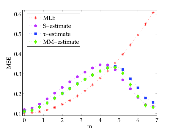
Figure 1: Simulation: mean squared errors for q=2๐‘ž2q=2 and x0=1subscript๐‘ฅ01x_{0}=1.
Refer to caption
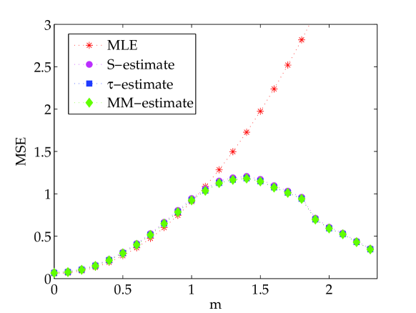
Figure 2: Simulation: mean squared errors for q=2๐‘ž2q=2 and x0=10subscript๐‘ฅ010x_{0}=10.
Refer to caption
Figure 3: Simulation: mean squared errors for q=5๐‘ž5q=5 and x0=1subscript๐‘ฅ01x_{0}=1.
Refer to caption
Figure 4: Simulation: mean squared errors for q=5๐‘ž5q=5 and x0=10subscript๐‘ฅ010x_{0}=10.

In Figures 1, 2, 3 and 4 we show the MSEs of the different estimates under contamination.

In Figure 1, which corresponds to q=2๐‘ž2q=2 and x0=1subscript๐‘ฅ01x_{0}=1, we observe that the MM- and ฯ„๐œ\tau-estimates behave similarly, both having a smaller MSE than the S-estimate except when m๐‘šm is (approximately) between 2.82.82.8 and 444. In this case, the S-estimate has the largest maximum MSE among the robust estimates. As expected, the MSE of the MLE increases without bound for large m๐‘šm. Figure 2 shows the results for q=2๐‘ž2q=2 and x0=10subscript๐‘ฅ010x_{0}=10. S-, ฯ„๐œ\tau- and MM-estimates behave similarly. In Figure 3, which corresponds to q=5๐‘ž5q=5 and x0=1subscript๐‘ฅ01x_{0}=1, the three robust estimates are seen to follow essentially the same pattern. For mโ‰ค4.8๐‘š4.8m\leq 4.8 (approximately) the ฯ„๐œ\tau- and MM- estimates have similar behaviors, both outperforming the S-estimate. For m>4.8๐‘š4.8m>4.8 the S- and MM-estimates have similar behaviors, both outperforming the ฯ„๐œ\tau-estimate. For q=5๐‘ž5q=5 and x0=10subscript๐‘ฅ010x_{0}=10 (figure 4) the behavior of the robust estimates is similar to the one observed for q=2๐‘ž2q=2 and x0=10subscript๐‘ฅ010x_{0}=10 (figure 2).

9 An example with real data

In this Section we analyze a dataset corresponding to electron-probe X ray microanalysis of archeological glass vessels (Janssens et al., [12]). For each of n=180๐‘›180n=180 vessels we have a spectrum on 1920 frequencies and the contents of 13 chemical compounds; the purpose is to predict the contents on the basis of the spectra. In order to limit the size of our data set, we considered only two compounds (responses): P2O5 and PbO; and chose 12 equispaced frequencies between 100 to 400. This interval was chosen because the values of xiโ€‹jsubscript๐‘ฅ๐‘–๐‘—x_{ij} are almost null for frequencies below 100 and above 400. We have therefore p=13๐‘13p=13 and q=2๐‘ž2q=2.

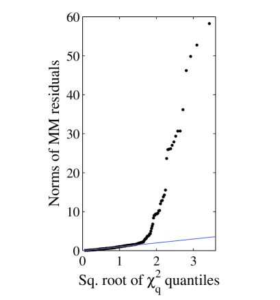
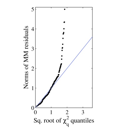
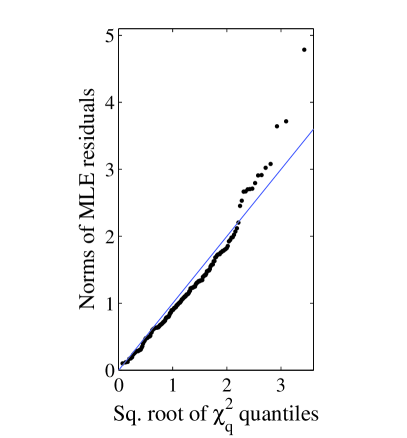
We considered two multivariate regression estimates: the MLE and our MM-estimate. As initial estimate for the MM-estimate we use an S-estimate. The S- and the MM-estimates employ bisquare ฯ๐œŒ\rho-functions with constants such that the MM-estimate has Gaussian ARE equal to 0.95 and the S-estimate has breakdown point 0.5. In Figure 5 we present QQ-plots of the Mahalanobis norms of the residuals of the MLE and the MM-estimate against the root quantiles of the chi-squared distribution with q๐‘žq degrees of freedom. The QQ-plot of the MM-estimate shows clear outliers.

Refer to captionRefer to captionRefer to caption
Figure 5: QQ-plots of the Mahalanobis norms of the residuals of the MM-estimate (left), the MLE (right) and the MM-estimate in the same interval as the MLE (center).
Refer to captionRefer to caption
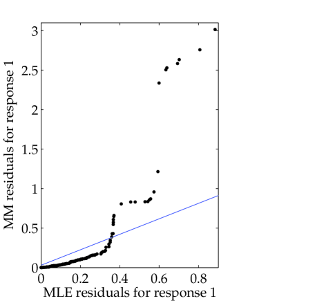
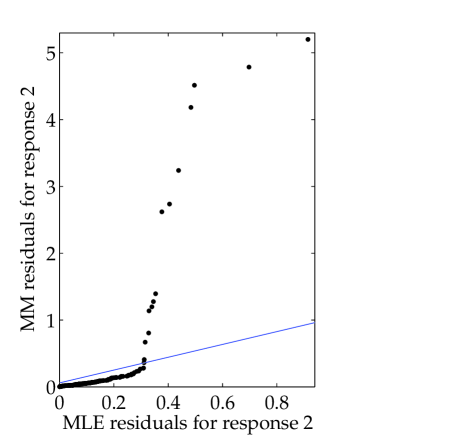
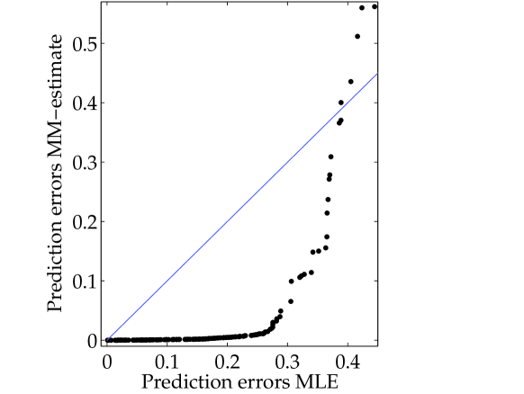
Figure 6: QQ-plots of sorted absolute residuals of MM-estimates vs sorted absolute residuals of MLE for each component of the response. Left plot corresponds to P2O5 (first component) and right to PbO (second component).
ย ย ย ย ย ย ย ย ย ย ย ย ย ย ย MLE ย ย ย ย ย ย ย ย ย ย ย MM-estimate
(0.0645โˆ’0.0008โˆ’0.00080.0348)0.06450.00080.00080.0348\left(\begin{array}[pos]{cc}0.0645&-0.0008\\ -0.0008&0.0348\end{array}\right) (0.0102โˆ’0.0014โˆ’0.00140.0084)0.01020.00140.00140.0084\left(\begin{array}[pos]{cc}0.0102&-0.0014\\ -0.0014&0.0084\end{array}\right)
Table 4: MLE and MM-estimate of the covariance matrix of the errors.
Criterion ย ย ย ย ย ย ย MLE ฯ„๐œ\tau-estimate MM-estimate MM-univariate
Component 1 2 1 2 1 2 1ย ย ย ย ย ย ย ย ย 2
MSE 0.081 0.051 0.351 0.806 0.340 0.682 0.354ย ย ย ย 0.762
ฯ„๐œ\tau-scale 0.044 0.022 0.005 0.007 0.008 0.006 0.005ย ย ย ย 0.006
Table 5: Mean square error (MSE) and ฯ„๐œ\tau-scale of the prediction errors of the MLE, multivariate MM-estimate, ฯ„๐œ\tau-estimate and univariate MM-estimate for each component of the response, computed by cross-validation.

In Figure 6 are compared the sorted absolute values of the residuals of the MLE with those corresponding to the MM-estimator for each component of the response.

The right and left panels of Figure 5 show respectively the QQ-plots of the Mahalanobis norms of the residuals of the MLE and the MM-estimate against the square root quantiles of the chi-squared distribution with q๐‘žq degrees of freedom. For ease of comparison, the center panel shows the MMโ€™s QQ-plot truncated to the size of the MLEโ€™s QQ-plot. The latter shows a very good fit of the norms to the chi-squared distribution, and therefore points out no suspect points, while the MM-estimateโ€™s QQ-plot indicates some 30 possible outliers, i.e. about 16%percent\% of the data.

The MLEโ€™s norms are in general smaller than the MM-estimateโ€™s norms, but this does not mean that the former gives a better fit, since here the residuals are normalized by the respective estimated residual dispersion matrices ๐šบ^0subscript^๐šบ0\widehat{\mathbf{\Sigma}}_{0}. Figure 6 compares the sorted absolute values of the (univariate) residuals of the MLE with those of the MM-estimate for each response. We can see that the majority of the residuals corresponding to the MM-estimate are smaller than those of the MLE.

To understand why the MLEโ€™s norms are in general smaller than the MM-estimateโ€™s norms, while the respective residuals are in general smaller, we show in Table 4 the estimates given by the MLE and MM-estimate of the dispersion matrix of the errors. It is seen that the former is โ€œmuch largerโ€ than the latter, in that its two diagonal elements are respectively six and four times those of the latter.

Refer to captionRefer to caption
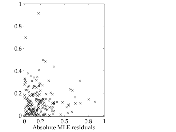
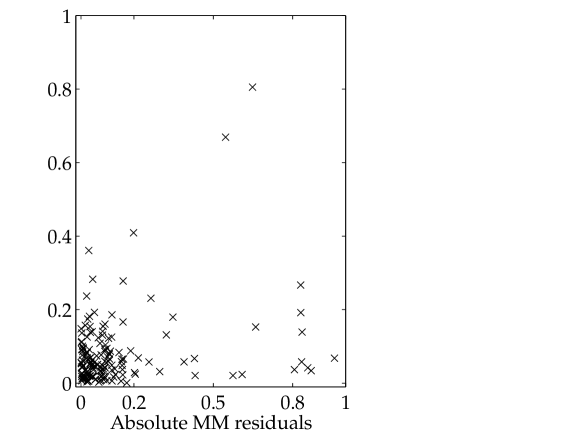
Figure 7: Absolute values of the coordinates of the bidimensional residual vectors corresponding to the MLE (left) and to the MM-estimate (right).

To complete the description of the estimatesโ€™ fit, Figure 7 shows the absolute values of the coordinates of the bidimensional residual vectors, in the right panel (corresponding to residuals of the MM-estimate) is truncated to the size of the left panel (corresponding to residuals of the MLE), and consequently a 10%percent\% of the absolute residuals of the MM-estimate is not shown. It is seen that, while the residuals from MM have a larger range than those from the MLE, they are in general more concentrated near the origin. In general, we may conclude that the MM-estimate gives a good fit to the bulk of the data, at the expense of misfitting a reduced proportion of atypical points, while the MLE tries to fit all data points, including the atypical ones, with the cost of a poor fit to the bulk of the data.

We compared the predictive behaviors of the MLE and the MM-estimates through five-fold cross validation. We also included the univariate MM-estimates corresponding to each component of the response and the ฯ„๐œ\tau-estimate proposed by Garcรญa Ben et al. [8]. As initial estimate for the univariate MM-estimates we use S-estimates. The ฯ„๐œ\tau-, S- and the univariate MM-estimates employ bisquare ฯ๐œŒ\rho-functions with constants such that the univariate MM- and ฯ„๐œ\tau-estimates have Gaussian ARE equal to 0.95 and the S-estimate has breakdown point 0.5. We considered two evaluation criteria: the mean squared error (MSE) and a robust criterion, namely a ฯ„๐œ\tau-scale (8.2) of the predictive errors, both computed separately for each component of the response. In the ฯ„๐œ\tau-scale s๐‘ s is an M-scale with breakdown point 0.5 and ฯ2subscript๐œŒ2\rho_{2} is a bisquare ฯ๐œŒ\rho-function with constant such that the ฯ„๐œ\tau-scale has Gaussian asymptotic efficiency equal to 0.85.

Table 5 shows the results. According to the MSE, the MLE is much better than the robust estimates. However, the ฯ„๐œ\tau-scales yield the opposite conclusion. The reason of this fact is the MSEโ€™s sensitivity to outliers. This result shows how misleading a non-robust criterion may be. According to the ฯ„๐œ\tau-scale, the predictive performance of our MM-estimate for the second component is slightly better than that of the ฯ„๐œ\tau-estimate, while the opposite occurs for the first component. The results obtained with the univariate MM-estimates are similar to those of the multivariate MM.

Refer to captionRefer to caption
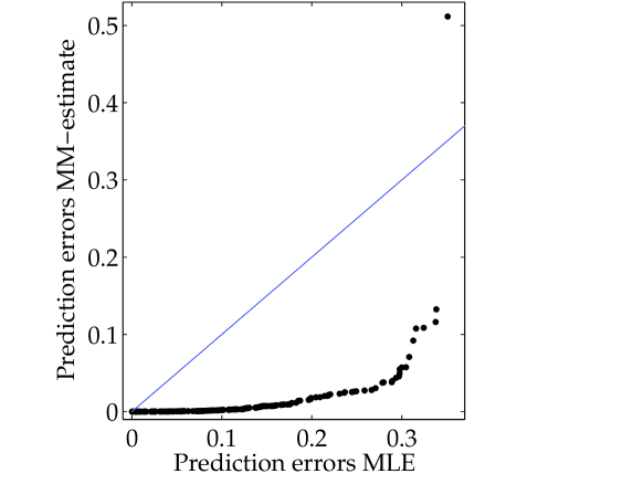
Figure 8: QQ-plots of sorted absolute prediction errors of MM-estimates vs sorted absolute prediction errors of MLE for each component of the response, computed by cross-validation. Left plot corresponds to P2O5 (first component) and right to PbO (second component).

The QQ-plots in Figure 8 compare for each response component the absolute values of the sorted cross validation prediction errors of our MM-estimate with those of the MLE. For reasons of scale, in each QQ-plot the observations with the 12 largest absolute prediction errors were omitted. We can see that most points lie below the identity line representing the identity function, showing that the MM-estimate provides a better prediction for the bulk of the data.

10 Conclusions

In this paper we have presented MM-estimates for the multivariate linear model and showed that they maintain the same good theoretical properties as in the univariate case, such as a high breakdown point and high Gaussian efficiency. The simulation study indicates that it has the desired high efficiency, and that its behavior is in general similar, and in several situations superior, to that of the ฯ„๐œ\tau-estimate; it is also more efficient, and in most situations more robust, than the S-estimate. In the example with real data, our MM-estimate gives a good fit to the bulk of the data, pointing out the existence of atypical points, and shows a good predictive behavior.

Appendix A Appendix

Before showing some of the properties of the MM-estimate, we set the notation for norms of vectors and matrices that we will use later:

Given ๐ฏโˆˆโ„m๐ฏsuperscriptโ„๐‘š\mathbf{v}\in\mathbb{R}^{m}, we denote its 2-norm or Euclidean norm as:

โ€–๐ฏโ€–=โ€–๐ฏโ€–2=(โˆ‘i=1mvi2)1/2,norm๐ฏsubscriptnorm๐ฏ2superscriptsuperscriptsubscript๐‘–1๐‘šsuperscriptsubscript๐‘ฃ๐‘–212\|\mathbf{v}\|=\|\mathbf{v}\|_{2}=\left(\sum_{i=1}^{m}v_{i}^{2}\right)^{1/2},

where visubscript๐‘ฃ๐‘–v_{i} represents the i๐‘–ith element of ๐ฏ๐ฏ\mathbf{v}.

Given a matrix ๐€โˆˆโ„rร—m๐€superscriptโ„๐‘Ÿ๐‘š\mathbf{A}\in\mathbb{R}^{r\times m}, its spectral norm โˆฅโ‹…โˆฅsโ€‹p\|\cdot\|_{sp}, is defined as follows:

โ€–๐€โ€–=โ€–๐€โ€–sโ€‹pnorm๐€subscriptnorm๐€๐‘ ๐‘\displaystyle\|\mathbf{A}\|=\|\mathbf{A}\|_{sp} =maxโก{โ€–๐€๐ฏโ€–:๐ฏโˆˆโ„mโ€‹ย withย โ€‹โ€–๐ฏโ€–=1}absent:norm๐€๐ฏ๐ฏsuperscriptโ„๐‘šย withย norm๐ฏ1\displaystyle=\max\{\|\mathbf{A}\mathbf{v}\|:\mathbf{v}\in\mathbb{R}^{m}\mbox{ with }\|\mathbf{v}\|=1\}
=maxโก{โ€–๐€๐ฏโ€–โ€–๐ฏโ€–:๐ฏโˆˆโ„mโ€‹ย withย โ€‹๐ฏโ‰ 0}.absent:norm๐€๐ฏnorm๐ฏ๐ฏsuperscriptโ„๐‘šย withย ๐ฏ0\displaystyle=\max\left\{\frac{\|\mathbf{A}\mathbf{v}\|}{\|\mathbf{v}\|}:\mathbf{v}\in\mathbb{R}^{m}\mbox{ with }\mathbf{v}\neq 0\right\}. (A.1)

Its 2-norm or Frobenius norm โˆฅโ‹…โˆฅ2\|\cdot\|_{2} is its Euclidean norm if we think the matrix ๐€๐€\mathbf{A} as a vector of โ„m.rsuperscriptโ„formulae-sequence๐‘š๐‘Ÿ\mathbb{R}^{m.r}, i.e.

โ€–๐€โ€–2=[trโ€‹(๐€โ€ฒโ€‹๐€)]1/2=(โˆ‘i=1mโˆ‘j=1n|aiโ€‹j|2)1/2,subscriptnorm๐€2superscriptdelimited-[]trsuperscript๐€โ€ฒ๐€12superscriptsuperscriptsubscript๐‘–1๐‘šsuperscriptsubscript๐‘—1๐‘›superscriptsubscript๐‘Ž๐‘–๐‘—212\|\mathbf{A}\|_{2}=\left[\text{tr}(\mathbf{A}^{\prime}\mathbf{A})\right]^{1/2}=\left(\sum_{i=1}^{m}\sum_{j=1}^{n}|a_{ij}|^{2}\right)^{1/2}, (A.2)

where aiโ€‹jsubscript๐‘Ž๐‘–๐‘—a_{ij} represents to the (i,j)๐‘–๐‘—(i,j)th element of the matrix ๐€๐€\mathbf{A} and trโ€‹(โ‹…)trโ‹…\text{tr}(\cdot) denotes the trace.

Given ๐•โˆˆโ„mร—m๐•superscriptโ„๐‘š๐‘š\mathbf{V}\in\mathbb{R}^{m\times m} we denote its eigenvalues as

ฮป1โ€‹(๐•)โ‰ฅโ€ฆโ‰ฅฮปmโ€‹(๐•),subscript๐œ†1๐•โ€ฆsubscript๐œ†๐‘š๐•\lambda_{1}(\mathbf{V})\geq\ldots\geq\lambda_{m}(\mathbf{V}),

then if ๐•๐•\mathbf{V} is positive definite

โ€–๐•โ€–=maxjโก{ฮปjโ€‹(๐•)}=ฮป1โ€‹(๐•).norm๐•subscript๐‘—subscript๐œ†๐‘—๐•subscript๐œ†1๐•\|\mathbf{V}\|=\max_{j}\{\lambda_{j}(\mathbf{V})\}=\lambda_{1}(\mathbf{V}). (A.3)
Remark 6.

Recall also that for any two norms ||โ‹…||a||\cdot||_{a} and ||โ‹…||b||\cdot||_{b}, we have that

ฮฑโ€‹โ€–๐€โ€–aโ‰คโ€–๐€โ€–bโ‰คฮฒโ€‹โ€–๐€โ€–ฮฑ๐›ผsubscriptnorm๐€๐‘Žsubscriptnorm๐€๐‘๐›ฝsubscriptnorm๐€๐›ผ\alpha\left\|\mathbf{A}\right\|_{a}\leq\left\|\mathbf{A}\right\|_{b}\leq\beta\left\|\mathbf{A}\right\|_{\alpha}

for some ฮฑ๐›ผ\alpha and ฮฒ๐›ฝ\beta and for all matrices ๐€โˆˆโ„rร—m๐€superscriptโ„๐‘Ÿ๐‘š\mathbf{A}\in\mathbb{R}^{r\times m}. In other words, they are equivalent norms, i.e. they induce the same topology in โ„rร—msuperscriptโ„๐‘Ÿ๐‘š\mathbb{R}^{r\times m}. For ||โ‹…||a=||โ‹…||||\cdot||_{a}=||\cdot|| and ||โ‹…||b=||โ‹…||2||\cdot||_{b}=||\cdot||_{2} we have ฮฑ=1๐›ผ1\alpha=1 and ฮฒ=k๐›ฝ๐‘˜\beta=\sqrt{k} where k๐‘˜k is the rank of the matrix ๐€๐€\mathbf{A}.

Recall also that spectral norm and the Frobenius norm are matrix norms, i.e., for any pair of matrices in โ„mร—msuperscriptโ„๐‘š๐‘š\mathbb{R}^{m\times m} ๐€๐€\mathbf{A} and ๐๐\mathbf{B}

โ€–๐€๐โ€–2โ‰คโ€–๐€โ€–2โ€‹โ€–๐โ€–2โ€‹ย andย โ€‹โ€–๐€๐โ€–โ‰คโ€–๐€โ€–โ€‹โ€–๐โ€–.subscriptnorm๐€๐2subscriptnorm๐€2subscriptnorm๐2ย andย norm๐€๐norm๐€norm๐\|\mathbf{A}\mathbf{B}\|_{2}\leq\|\mathbf{A}\|_{2}\|\mathbf{B}\|_{2}\;\;\text{ and }\;\;\|\mathbf{A}\mathbf{B}\|\leq\|\mathbf{A}\|\|\mathbf{B}\|. (A.4)

This property will be used in several times.


Before proving Theorem 1 we will prove the following Lemma:

Lemma 9.

Let ๐ฒโˆˆโ„q๐ฒsuperscriptโ„๐‘ž\mathbf{y}\in\mathbb{R}^{q} and ๐ฑโˆˆโ„p๐ฑsuperscriptโ„๐‘\mathbf{x}\in\mathbb{R}^{p} be fixed vectors. The function

d2โ€‹(๐,๐šบ)=(๐ฒโˆ’๐โ€ฒโ€‹๐ฑ)โ€ฒโ€‹๐šบโˆ’1โ€‹(๐ฒโˆ’๐โ€ฒโ€‹๐ฑ)superscript๐‘‘2๐๐šบsuperscript๐ฒsuperscript๐โ€ฒ๐ฑโ€ฒsuperscript๐šบ1๐ฒsuperscript๐โ€ฒ๐ฑd^{2}(\mathbf{B},\mathbf{\Sigma})=(\mathbf{y}-\mathbf{B}^{\prime}\mathbf{x})^{\prime}\mathbf{\Sigma}^{-1}(\mathbf{y}-\mathbf{B}^{\prime}\mathbf{x})

is continuous in โ„pร—qร—๐’ฎqsuperscriptโ„๐‘๐‘žsubscript๐’ฎ๐‘ž\mathbb{R}^{p\times q}\times\mathcal{S}_{q}.

Proof: We only give the main ideas of the proof. Without loss of generality, due to Remark 6, we can consider in โ„pร—qร—โ„qร—qsuperscriptโ„๐‘๐‘žsuperscriptโ„๐‘ž๐‘ž\mathbb{R}^{p\times q}\times\mathbb{R}^{q\times q} the topology induced by the norm

โ€–|(๐€,๐•)โ€–|=sup{โ€–๐€โ€–2,โ€–๐•โ€–}.delimited-โ€–|delimited-|โ€–๐€๐•supremumsubscriptnorm๐€2norm๐•\||(\mathbf{A},\mathbf{V})\||=\sup\{\|\mathbf{A}\|_{2},\|\mathbf{V}\|\}. (A.5)

Given (๐0,๐šบ0)subscript๐0subscript๐šบ0(\mathbf{B}_{0},\mathbf{\Sigma}_{0}) in โ„pร—qร—โ„qร—qsuperscriptโ„๐‘๐‘žsuperscriptโ„๐‘ž๐‘ž\mathbb{R}^{p\times q}\times\mathbb{R}^{q\times q}, the proof consists in find an upper bound of |d2โ€‹(๐,๐šบ)โˆ’d2โ€‹(๐0,๐šบ0)|superscript๐‘‘2๐๐šบsuperscript๐‘‘2subscript๐0subscript๐šบ0\left|d^{2}(\mathbf{B},\mathbf{\Sigma})-d^{2}(\mathbf{B}_{0},\mathbf{\Sigma}_{0})\right| that tends to 00 when โ€–|(๐,๐šบ)โˆ’(๐0,๐šบ0)โ€–|โ†’0.โ†’delimited-โ€–|delimited-|โ€–๐๐šบsubscript๐0subscript๐šบ00\||(\mathbf{B},\mathbf{\Sigma})-(\mathbf{B}_{0},\mathbf{\Sigma}_{0})\||\rightarrow 0.

Adding and subtracting d2โ€‹(๐0,๐šบ)superscript๐‘‘2subscript๐0๐šบd^{2}(\mathbf{B}_{0},\mathbf{\Sigma}) we have that

|d2โ€‹(๐,๐šบ)โˆ’d2โ€‹(๐0,๐šบ0)|superscript๐‘‘2๐๐šบsuperscript๐‘‘2subscript๐0subscript๐šบ0\displaystyle\left|d^{2}(\mathbf{B},\mathbf{\Sigma})-d^{2}(\mathbf{B}_{0},\mathbf{\Sigma}_{0})\right| โ‰ค\displaystyle\leq |d2โ€‹(๐,๐šบ)โˆ’d2โ€‹(๐0,๐šบ)|+|d2โ€‹(๐0,๐šบ)โˆ’d2โ€‹(๐0,๐šบ0)|.superscript๐‘‘2๐๐šบsuperscript๐‘‘2subscript๐0๐šบsuperscript๐‘‘2subscript๐0๐šบsuperscript๐‘‘2subscript๐0subscript๐šบ0\displaystyle\left|d^{2}(\mathbf{B},\mathbf{\Sigma})-d^{2}(\mathbf{B}_{0},\mathbf{\Sigma})\right|+\left|d^{2}(\mathbf{B}_{0},\mathbf{\Sigma})-d^{2}(\mathbf{B}_{0},\mathbf{\Sigma}_{0})\right|.

Let rโ€‹(๐0)=(๐ฒโˆ’๐0โ€ฒโ€‹๐ฑ)๐‘Ÿsubscript๐0๐ฒsuperscriptsubscript๐0โ€ฒ๐ฑr(\mathbf{B}_{0})=(\mathbf{y}-\mathbf{B}_{0}^{\prime}\mathbf{x}). Using basic tools from linear algebra we obtain

|d2โ€‹(๐,๐šบ)โˆ’d2โ€‹(๐0,๐šบ)|โ‰คqโ€‹โ€–|(๐,๐šบ)โˆ’(๐0,๐šบ0)โ€–|โ€‹(โ€–๐ฑโ€‹โ€–+2โ€–โ€‹rโ€‹(๐0)โ€–)โ€‹โ€–๐ฑโ€–โ€‹ฮป1โ€‹(๐šบโˆ’1),superscript๐‘‘2๐๐šบsuperscript๐‘‘2subscript๐0๐šบ๐‘ždelimited-โ€–|delimited-|โ€–๐๐šบsubscript๐0subscript๐šบ0norm๐ฑnorm2๐‘Ÿsubscript๐0norm๐ฑsubscript๐œ†1superscript๐šบ1\left|d^{2}(\mathbf{B},\mathbf{\Sigma})-d^{2}(\mathbf{B}_{0},\mathbf{\Sigma})\right|\leq q\||(\mathbf{B},\mathbf{\Sigma})-(\mathbf{B}_{0},\mathbf{\Sigma}_{0})\||\left(\|\mathbf{x}\|+2\left\|r(\mathbf{B}_{0})\right\|\right)\|\mathbf{x}\|\lambda_{1}(\mathbf{\Sigma}^{-1}),

and by Weylโ€™s Perturbation Theorem (see [4], pg. 63), we have that

ฮป1โ€‹(๐šบโˆ’1)=1ฮปqโ€‹(๐šบ)<1ฮปqโ€‹(๐šบ0)โˆ’โ€–|(๐,๐šบ)โˆ’(๐0,๐šบ0)โ€–|,subscript๐œ†1superscript๐šบ11subscript๐œ†๐‘ž๐šบ1subscript๐œ†๐‘žsubscript๐šบ0delimited-โ€–|delimited-|โ€–๐๐šบsubscript๐0subscript๐šบ0\lambda_{1}(\mathbf{\Sigma}^{-1})=\frac{1}{\lambda_{q}(\mathbf{\Sigma})}<\frac{1}{\lambda_{q}(\mathbf{\Sigma}_{0})-\||(\mathbf{B},\mathbf{\Sigma})-(\mathbf{B}_{0},\mathbf{\Sigma}_{0})\||}, (A.6)

combining these inequalities we obtain a bound of |d2โ€‹(๐,๐šบ)โˆ’d2โ€‹(๐0,๐šบ)|superscript๐‘‘2๐๐šบsuperscript๐‘‘2subscript๐0๐šบ\left|d^{2}(\mathbf{B},\mathbf{\Sigma})-d^{2}(\mathbf{B}_{0},\mathbf{\Sigma})\right| that tends to 00 when โ€–|(๐,๐šบ)โˆ’(๐0,๐šบ0)โ€–|โ†’0.โ†’delimited-โ€–|delimited-|โ€–๐๐šบsubscript๐0subscript๐šบ00\||(\mathbf{B},\mathbf{\Sigma})-(\mathbf{B}_{0},\mathbf{\Sigma}_{0})\||\rightarrow 0.

If rโ€‹(๐0)=๐ŸŽ๐‘Ÿsubscript๐00r(\mathbf{B}_{0})=\mathbf{0} the lemma is proved, otherwise using the Cauchy-Schwarz inequality and (A.6) we have

|d2โ€‹(๐0,๐šบ)โˆ’d2โ€‹(๐0,๐šบ0)|โ‰คโ€–๐šบ0โˆ’1โ€–โ€‹โ€–rโ€‹(๐0)โ€–2โ€‹โ€–|(๐,๐šบ)โˆ’(๐0,๐šบ0)โ€–|ฮปqโ€‹(๐šบ0)โˆ’โ€–|(๐,๐šบ)โˆ’(๐0,๐šบ0)โ€–|,superscript๐‘‘2subscript๐0๐šบsuperscript๐‘‘2subscript๐0subscript๐šบ0normsuperscriptsubscript๐šบ01superscriptnorm๐‘Ÿsubscript๐02delimited-โ€–|delimited-|โ€–๐๐šบsubscript๐0subscript๐šบ0subscript๐œ†๐‘žsubscript๐šบ0delimited-โ€–|delimited-|โ€–๐๐šบsubscript๐0subscript๐šบ0\displaystyle\left|d^{2}(\mathbf{B}_{0},\mathbf{\Sigma})-d^{2}(\mathbf{B}_{0},\mathbf{\Sigma}_{0})\right|\leq\frac{\|\mathbf{\Sigma}_{0}^{-1}\|\|r(\mathbf{B}_{0})\|^{2}\||(\mathbf{B},\mathbf{\Sigma})-(\mathbf{B}_{0},\mathbf{\Sigma}_{0})\||}{\lambda_{q}(\mathbf{\Sigma}_{0})-\||(\mathbf{B},\mathbf{\Sigma})-(\mathbf{B}_{0},\mathbf{\Sigma}_{0})\||},

which completes the proof. โ– โ– \blacksquare

Proof of Theorem 1: By Lemma 9, it sufices to show that there exist t1subscript๐‘ก1t_{1} and t2subscript๐‘ก2t_{2} such that

inf(๐,๐šช)โˆˆ๐’žโˆ‘i=1nฯโ€‹(diโ€‹(๐,๐šช)ฯƒ^n)>โˆ‘i=1nฯโ€‹(diโ€‹(๐~n,๐šช~n)ฯƒ^n)subscriptinfimum๐๐šช๐’žsuperscriptsubscript๐‘–1๐‘›๐œŒsubscript๐‘‘๐‘–๐๐šชsubscript^๐œŽ๐‘›superscriptsubscript๐‘–1๐‘›๐œŒsubscript๐‘‘๐‘–subscript~๐๐‘›subscript~๐šช๐‘›subscript^๐œŽ๐‘›\displaystyle{\inf_{(\mathbf{B},\mathbf{\Gamma})\in\mathcal{C}}\sum_{i=1}^{n}\rho\left(\frac{d_{i}(\mathbf{B},\mathbf{\Gamma})}{\hat{\sigma}_{n}}\right)>\sum_{i=1}^{n}\rho\left(\frac{d_{i}(\widetilde{\mathbf{B}}_{n},\widetilde{\mathbf{\Gamma}}_{n})}{\hat{\sigma}_{n}}\right)} (A.7)

where

๐’ž={(๐,๐šช)โˆˆโ„pร—qร—๐’ฎqย withย |๐šช|=1:ฮปq(๐šช)โ‰คt1ย orย โˆฅ๐โˆฅ2โ‰ฅt2}.\mathcal{C}=\{(\mathbf{B},\mathbf{\Gamma})\in\mathbb{R}^{p\times q}\times\mathcal{S}_{q}\text{ with }|\mathbf{\Gamma}|=1:\lambda_{q}(\mathbf{\Gamma})\leq t_{1}\text{ or }\|\mathbf{B}\|_{2}\geq t_{2}\}. (A.8)

By definition of knsubscript๐‘˜๐‘›k_{n} we have that for all ๐œฝโˆˆโ„p+q๐œฝsuperscriptโ„๐‘๐‘ž\boldsymbol{\theta}\in\mathbb{R}^{p+q}

โ™ฏโ€‹{i:|๐œฝโ€ฒโ€‹๐ณi|>0}/nโ‰ฅ1โˆ’(kn/n).โ™ฏconditional-set๐‘–superscript๐œฝโ€ฒsubscript๐ณ๐‘–0๐‘›1subscript๐‘˜๐‘›๐‘›\sharp\{i:|\boldsymbol{\theta}^{\prime}\mathbf{z}_{i}|>0\}/n\geq 1-(k_{n}/n).

Taking 0.5<ฮด<1โˆ’(kn/n)5๐›ฟ1subscript๐‘˜๐‘›๐‘›5<\delta<1-(k_{n}/n) and using a compactness argument we can find ฮต>0๐œ€0\varepsilon>0 such that

infโ€–๐œฝโ€–=1โ™ฏโ€‹{i:|๐œฝโ€ฒโ€‹๐ณi|>ฮต}/nโ‰ฅฮด.subscriptinfimumnorm๐œฝ1โ™ฏconditional-set๐‘–superscript๐œฝโ€ฒsubscript๐ณ๐‘–๐œ€๐‘›๐›ฟ\displaystyle{\inf_{\boldsymbol{\|\theta}\|=1}\sharp\{i:|\boldsymbol{\theta}^{\prime}\mathbf{z}_{i}|>\varepsilon\}/n\geq\delta.} (A.9)

Let (๐,๐šช)โˆˆโ„pร—qร—๐’ฎq๐๐šชsuperscriptโ„๐‘๐‘žsubscript๐’ฎ๐‘ž(\mathbf{B},\mathbf{\Gamma})\in\mathbb{R}^{p\times q}\times\mathcal{S}_{q} be such that |๐šช|=1๐šช1|\mathbf{\Gamma}|=1, ๐šซ๐šซ\boldsymbol{\Delta} be the diagonal matrix of eigenvalues of ๐šช๐šช\mathbf{\Gamma} order from lowest to highest and ๐”๐”\mathbf{U} be the orthonormal matrix of eigenvectors of ๐šช๐šช\mathbf{\Gamma} which verifies ๐šช=๐”โ€‹๐šซโ€‹๐”โ€ฒ๐šช๐”๐šซsuperscript๐”โ€ฒ\mathbf{\Gamma}=\mathbf{U}\boldsymbol{\Delta}\mathbf{U}^{\prime}. Then

di2โ€‹(๐,๐šช)superscriptsubscript๐‘‘๐‘–2๐๐šช\displaystyle d_{i}^{2}(\mathbf{B},\mathbf{\Gamma}) =\displaystyle= (๐ฒiโˆ’๐โ€ฒโ€‹๐ฑi)โ€ฒโ€‹๐šชโˆ’1โ€‹(๐ฒiโˆ’๐โ€ฒโ€‹๐ฑi)superscriptsubscript๐ฒ๐‘–superscript๐โ€ฒsubscript๐ฑ๐‘–โ€ฒsuperscript๐šช1subscript๐ฒ๐‘–superscript๐โ€ฒsubscript๐ฑ๐‘–\displaystyle(\mathbf{y}_{i}-\mathbf{B}^{\prime}\mathbf{x}_{i})^{\prime}\mathbf{\Gamma}^{-1}(\mathbf{y}_{i}-\mathbf{B}^{\prime}\mathbf{x}_{i}) (A.10)
=\displaystyle= (๐”โ€ฒโ€‹๐ฒiโˆ’๐”โ€ฒโ€‹๐โ€ฒโ€‹๐ฑi)โ€ฒโ€‹๐šซโˆ’1โ€‹(๐”โ€ฒโ€‹๐ฒiโˆ’๐”โ€ฒโ€‹๐โ€ฒโ€‹๐ฑi)โ‰ฅ(๐žโ€ฒโ€‹๐ณi)2ฮปqโ€‹(๐šช),superscriptsuperscript๐”โ€ฒsubscript๐ฒ๐‘–superscript๐”โ€ฒsuperscript๐โ€ฒsubscript๐ฑ๐‘–โ€ฒsuperscript๐šซ1superscript๐”โ€ฒsubscript๐ฒ๐‘–superscript๐”โ€ฒsuperscript๐โ€ฒsubscript๐ฑ๐‘–superscriptsuperscript๐žโ€ฒsubscript๐ณ๐‘–2subscript๐œ†๐‘ž๐šช\displaystyle(\mathbf{U}^{\prime}\mathbf{y}_{i}-\mathbf{U}^{\prime}\mathbf{B}^{\prime}\mathbf{x}_{i})^{\prime}\mathbf{\Delta}^{-1}(\mathbf{U}^{\prime}\mathbf{y}_{i}-\mathbf{U}^{\prime}\mathbf{B}^{\prime}\mathbf{x}_{i})\geq\frac{(\mathbf{e}^{\prime}\mathbf{z}_{i})^{2}}{\lambda_{q}(\mathbf{\Gamma})},

with ๐ž=(โˆ’๐ฏ1,๐Š1)๐žsubscript๐ฏ1subscript๐Š1\mathbf{e}=(-\mathbf{v}_{1},\boldsymbol{\upsilon}_{1}) where ๐Š1subscript๐Š1\boldsymbol{\upsilon}_{1} and ๐ฏ1subscript๐ฏ1\mathbf{v}_{1} are the first row of ๐”โ€ฒsuperscript๐”โ€ฒ\mathbf{U}^{\prime} and ๐•=๐”โ€ฒโ€‹๐โ€ฒ๐•superscript๐”โ€ฒsuperscript๐โ€ฒ\mathbf{V}=\mathbf{U}^{\prime}\mathbf{B}^{\prime}, respectively.

Since โ€–๐žโ€–โ‰ฅ1norm๐ž1\|\mathbf{e}\|\geq 1, by (A.9) we have at least nโ€‹ฮด๐‘›๐›ฟn\delta values of diโ€‹(๐,๐šช)subscript๐‘‘๐‘–๐๐šชd_{i}(\mathbf{B},\mathbf{\Gamma}) greater or equal than ฮต/ฮปqโ€‹(๐šช).๐œ€subscript๐œ†๐‘ž๐šช\varepsilon/\sqrt{\lambda_{q}(\mathbf{\Gamma})}. Hence

โˆ‘i=1nฯ1โ€‹(diโ€‹(๐,๐šช)ฯƒ^n)โ‰ฅnโ€‹ฮดโ€‹ฯ1โ€‹(ฮตฯƒ^nโ€‹ฮปqโ€‹(๐šช)).superscriptsubscript๐‘–1๐‘›subscript๐œŒ1subscript๐‘‘๐‘–๐๐šชsubscript^๐œŽ๐‘›๐‘›๐›ฟsubscript๐œŒ1๐œ€subscript^๐œŽ๐‘›subscript๐œ†๐‘ž๐šช\sum_{i=1}^{n}\rho_{1}\left(\frac{d_{i}(\mathbf{B},\mathbf{\Gamma})}{\hat{\sigma}_{n}}\right)\geq n\delta\rho_{1}\left(\frac{\varepsilon}{\hat{\sigma}_{n}\sqrt{\lambda_{q}(\mathbf{\Gamma})}}\right).

Let t๐‘กt be such that ฯ1โ€‹(tฯƒ^n)=12โ€‹ฮด1subscript๐œŒ1๐‘กsubscript^๐œŽ๐‘›12subscript๐›ฟ1\displaystyle{\rho_{1}\left(\frac{t}{\hat{\sigma}_{n}}\right)=\frac{1}{2\delta_{1}}}, with 0.5<ฮด1<ฮด0.5subscript๐›ฟ1๐›ฟ0.5<\delta_{1}<\delta, and let t1=ฮต2t2subscript๐‘ก1superscript๐œ€2superscript๐‘ก2\displaystyle{t_{1}=\frac{\varepsilon^{2}}{t^{2}}}, then if ฮปqโ€‹(๐šช)โ‰คt1subscript๐œ†๐‘ž๐šชsubscript๐‘ก1\lambda_{q}(\mathbf{\Gamma})\leq t_{1} we obtain the inequality

โˆ‘i=1nฯ1โ€‹(diโ€‹(๐,๐šช)ฯƒ^n)โ‰ฅnโ€‹ฮดโ€‹ฯ1โ€‹(tฯƒ^n)>n2.superscriptsubscript๐‘–1๐‘›subscript๐œŒ1subscript๐‘‘๐‘–๐๐šชsubscript^๐œŽ๐‘›๐‘›๐›ฟsubscript๐œŒ1๐‘กsubscript^๐œŽ๐‘›๐‘›2\sum_{i=1}^{n}\rho_{1}\left(\frac{d_{i}(\mathbf{B},\mathbf{\Gamma})}{\hat{\sigma}_{n}}\right)\geq n\delta\rho_{1}\left(\frac{t}{\hat{\sigma}_{n}}\right)>\frac{n}{2}. (A.11)

If ฮปqโ€‹(๐šช)>t1subscript๐œ†๐‘ž๐šชsubscript๐‘ก1\lambda_{q}(\mathbf{\Gamma})>t_{1} and โ€–๐โ€–2โ‰ฅt2subscriptnorm๐2subscript๐‘ก2\|\mathbf{B}\|_{2}\geq t_{2}, all eigenvalues of ๐šช๐šช\mathbf{\Gamma} are smaller than 1/t1qโˆ’11superscriptsubscript๐‘ก1๐‘ž11/t_{1}^{q-1} and at least one column of ๐๐\mathbf{B} has a norm greater o equal than t2/qsubscript๐‘ก2๐‘žt_{2}/\sqrt{q}. By (A.2), we have

โ€–๐•โ€–22=โ€–๐”โ€ฒโ€‹๐โ€ฒโ€–22=trโ€‹(๐๐”๐”โ€ฒโ€‹๐โ€ฒ)=trโ€‹(๐๐โ€ฒ)=โ€–๐โ€ฒโ€–22=โ€–๐โ€–22,subscriptsuperscriptnorm๐•22subscriptsuperscriptnormsuperscript๐”โ€ฒsuperscript๐โ€ฒ22trsuperscript๐๐”๐”โ€ฒsuperscript๐โ€ฒtrsuperscript๐๐โ€ฒsubscriptsuperscriptnormsuperscript๐โ€ฒ22subscriptsuperscriptnorm๐22\|\mathbf{V}\|^{2}_{2}=\|\mathbf{U}^{\prime}\mathbf{B}^{\prime}\|^{2}_{2}=\text{tr}(\mathbf{B}\mathbf{U}\mathbf{U}^{\prime}\mathbf{B}^{\prime})=\text{tr}(\mathbf{B}\mathbf{B}^{\prime})=\|\mathbf{B}^{\prime}\|^{2}_{2}=\|\mathbf{B}\|^{2}_{2},

and therefore exists a k๐‘˜k such that โ€–๐ฏkโ€–โ‰ฅt2/qnormsubscript๐ฏ๐‘˜subscript๐‘ก2๐‘ž\|\mathbf{v}_{k}\|\geq t_{2}/\sqrt{q} where ๐ฏksubscript๐ฏ๐‘˜\mathbf{v}_{k} is the k๐‘˜kth row of ๐•๐•\mathbf{V}.

Then proceeding as in (A.10) we obtain

di2โ€‹(๐,๐šช)โ‰ฅ(๐žkโ€ฒโ€‹๐ณi)2โ€‹t1qโˆ’1,superscriptsubscript๐‘‘๐‘–2๐๐šชsuperscriptsuperscriptsubscript๐ž๐‘˜โ€ฒsubscript๐ณ๐‘–2superscriptsubscript๐‘ก1๐‘ž1d_{i}^{2}(\mathbf{B},\mathbf{\Gamma})\geq(\mathbf{e}_{k}^{\prime}\mathbf{z}_{i})^{2}t_{1}^{q-1},

where ๐žk=(โˆ’๐ฏk,๐Šk)subscript๐ž๐‘˜subscript๐ฏ๐‘˜subscript๐Š๐‘˜\mathbf{e}_{k}=(-\mathbf{v}_{k},\boldsymbol{\upsilon}_{k}) and ๐Šksubscript๐Š๐‘˜\boldsymbol{\upsilon}_{k} is the k๐‘˜kth row of ๐”โ€ฒsuperscript๐”โ€ฒ\mathbf{U}^{\prime}.

By (A.9), at least nโ€‹ฮด๐‘›๐›ฟn\delta values of diโ€‹(๐,๐šช)subscript๐‘‘๐‘–๐๐šชd_{i}(\mathbf{B},\mathbf{\Gamma}) are greater or equal than ฮตโ€‹โ€–๐žkโ€–/t1qโˆ’1๐œ€normsubscript๐ž๐‘˜superscriptsubscript๐‘ก1๐‘ž1\varepsilon\|\mathbf{e}_{k}\|/\sqrt{t_{1}^{q-1}} and โ€–๐žkโ€–2=1+โ€–๐ฏkโ€–2โ‰ฅt22/qsuperscriptnormsubscript๐ž๐‘˜21superscriptnormsubscript๐ฏ๐‘˜2superscriptsubscript๐‘ก22๐‘ž\|\mathbf{e}_{k}\|^{2}=1+\|\mathbf{v}_{k}\|^{2}\geq t_{2}^{2}/q.

Then if we take t2=tฮตโ€‹q/t1qโˆ’1subscript๐‘ก2๐‘ก๐œ€๐‘žsuperscriptsubscript๐‘ก1๐‘ž1\displaystyle{t_{2}=\frac{t}{\varepsilon}\sqrt{{q}/{t_{1}^{q-1}}}} we obtain

โˆ‘i=1nฯ1โ€‹(diโ€‹(๐,๐šช)ฯƒ^n)โ‰ฅnโ€‹ฮดโ€‹ฯ1โ€‹(tฯƒ^n)=n2.superscriptsubscript๐‘–1๐‘›subscript๐œŒ1subscript๐‘‘๐‘–๐๐šชsubscript^๐œŽ๐‘›๐‘›๐›ฟsubscript๐œŒ1๐‘กsubscript^๐œŽ๐‘›๐‘›2\sum_{i=1}^{n}\rho_{1}\left(\frac{d_{i}(\mathbf{B},\mathbf{\Gamma})}{\hat{\sigma}_{n}}\right)\geq n\delta\rho_{1}\left(\frac{t}{\hat{\sigma}_{n}}\right)=\frac{n}{2}. (A.12)

Then by (A.11) and (A.12)

inf(๐,๐šช)โˆˆ๐’žโˆ‘i=1nฯ1โ€‹(diโ€‹(๐,๐šช)ฯƒ^n)โ‰ฅn2subscriptinfimum๐๐šช๐’žsuperscriptsubscript๐‘–1๐‘›subscript๐œŒ1subscript๐‘‘๐‘–๐๐šชsubscript^๐œŽ๐‘›๐‘›2\inf_{(\mathbf{B},\mathbf{\Gamma})\in\mathcal{C}}\sum_{i=1}^{n}\rho_{1}\left(\frac{d_{i}(\mathbf{B},\mathbf{\Gamma})}{\hat{\sigma}_{n}}\right)\geq\frac{n}{2}

and by (2.4) and (2.1)

โˆ‘i=1nฯ1โ€‹(diโ€‹(๐~n,๐šช~n)ฯƒ^n)โ‰คโˆ‘i=1nฯ0โ€‹(diโ€‹(๐~n,๐šช~n)ฯƒ^n)=n2,superscriptsubscript๐‘–1๐‘›subscript๐œŒ1subscript๐‘‘๐‘–subscript~๐๐‘›subscript~๐šช๐‘›subscript^๐œŽ๐‘›superscriptsubscript๐‘–1๐‘›subscript๐œŒ0subscript๐‘‘๐‘–subscript~๐๐‘›subscript~๐šช๐‘›subscript^๐œŽ๐‘›๐‘›2\sum_{i=1}^{n}\rho_{1}\left(\frac{d_{i}(\widetilde{\mathbf{B}}_{n},\widetilde{\mathbf{\Gamma}}_{n})}{\hat{\sigma}_{n}}\right)\leq\sum_{i=1}^{n}\rho_{0}\left(\frac{d_{i}(\widetilde{\mathbf{B}}_{n},\widetilde{\mathbf{\Gamma}}_{n})}{\hat{\sigma}_{n}}\right)=\frac{n}{2},

and this proves the Theorem. โ– โ– \blacksquare


Before proving Theorem 2 we will give some results on matrix derivatives that will be used later.

Let ๐›๐›\mathbf{b} be a vector and ๐•๐•\mathbf{V} be a symmetric matrix,

โˆ‚๐›โ€ฒโ€‹๐•๐›โˆ‚๐›โ€ฒ=2โ€‹๐›โ€ฒโ€‹๐•,superscript๐›โ€ฒ๐•๐›superscript๐›โ€ฒ2superscript๐›โ€ฒ๐•\displaystyle{\frac{\partial\mathbf{b^{\prime}Vb}}{\partial\mathbf{b}^{\prime}}=2\mathbf{b^{\prime}V}}, (A.13)

if ๐•๐•\mathbf{V} is nonsingular,

โˆ‚|๐•|โˆ‚๐•=|๐•|โ€‹๐•โˆ’1๐•๐•๐•superscript๐•1\displaystyle{\frac{\partial|\mathbf{V}|}{\partial\mathbf{V}}=|\mathbf{V}|\mathbf{V}^{-1}} (A.14)

and

โˆ‚๐›โ€ฒโ€‹๐•โˆ’๐Ÿโ€‹๐›โˆ‚๐•=โˆ’๐•โˆ’๐Ÿโ€‹๐›๐›โ€ฒโ€‹๐•โˆ’๐Ÿ.superscript๐›โ€ฒsuperscript๐•1๐›๐•superscript๐•1superscript๐›๐›โ€ฒsuperscript๐•1\displaystyle{\frac{\partial\mathbf{b^{\prime}\mathbf{V}^{-1}b}}{\partial\mathbf{V}}=-\mathbf{\mathbf{V}^{-1}bb^{\prime}\mathbf{V}^{-1}}}. (A.15)

For further details see Chapter 17 of [24].

Let (๐,๐šบ)โˆˆโ„pร—qร—๐’ฎq๐๐šบsuperscriptโ„๐‘๐‘žsubscript๐’ฎ๐‘ž(\mathbf{B},\mathbf{\Sigma})\in\mathbb{R}^{p\times q}\times\mathcal{S}_{q}, using vecโ€‹(๐โ€ฒโ€‹๐€)=(๐€โŠ—๐ˆq)โ€‹vecโ€‹(๐โ€ฒ)vecsuperscript๐โ€ฒ๐€tensor-product๐€subscript๐ˆ๐‘žvecsuperscript๐โ€ฒ\text{vec}(\mathbf{B}^{\prime}\mathbf{A})=(\mathbf{A}\otimes\mathbf{I}_{q})\text{vec}(\mathbf{B}^{\prime}), it is easy to check that

โˆ‚vecโ€‹(๐โ€ฒโ€‹๐€)โˆ‚vecโ€‹(๐โ€ฒ)โ€ฒ=(๐€โ€ฒโŠ—๐ˆq).vecsuperscript๐โ€ฒ๐€vecsuperscriptsuperscript๐โ€ฒโ€ฒtensor-productsuperscript๐€โ€ฒsubscript๐ˆ๐‘ž\frac{\partial\text{vec}(\mathbf{B}^{\prime}\mathbf{A})}{\partial\text{vec}(\mathbf{B}^{\prime})^{\prime}}=(\mathbf{A}^{\prime}\otimes\mathbf{I}_{q}). (A.16)

From (A.16) and (A.13) it follows that

โˆ‚dโ€‹(๐,๐šบ)โˆ‚vecโ€‹(๐โ€ฒ)โ€ฒ=โˆ’(๐ฒโˆ’๐โ€ฒโ€‹๐ฑ)โ€ฒโ€‹๐šบโˆ’1โ€‹(๐ฑโ€ฒโŠ—๐ˆq)dโ€‹(๐,๐šบ).๐‘‘๐๐šบvecsuperscriptsuperscript๐โ€ฒโ€ฒsuperscript๐ฒsuperscript๐โ€ฒ๐ฑโ€ฒsuperscript๐šบ1tensor-productsuperscript๐ฑโ€ฒsubscript๐ˆ๐‘ž๐‘‘๐๐šบ\frac{\partial d(\mathbf{B},\mathbf{\Sigma})}{\partial\text{vec}(\mathbf{B}^{\prime})^{\prime}}=-\frac{(\mathbf{y}-\mathbf{B}^{\prime}\mathbf{x})^{\prime}\mathbf{\Sigma}^{-1}(\mathbf{x}^{\prime}\otimes\mathbf{I}_{q})}{d(\mathbf{B},\mathbf{\Sigma})}. (A.17)

Proof of Theorem 2: The definition of MM-estimates can be reformulated, using the function ๐šชโ€‹(๐šบ):=๐šบ/|๐šบ|1/qassign๐šช๐šบ๐šบsuperscript๐šบ1๐‘ž\mathbf{\Gamma}(\mathbf{\Sigma}):=\mathbf{\Sigma}/|\mathbf{\Sigma}|^{1/q}, in the following way: let (๐^n,๐‚n)subscript^๐๐‘›subscript๐‚๐‘›(\widehat{\mathbf{B}}_{n},\mathbf{C}_{n}) be any local minimum of Sโˆ—โ€‹(๐,๐šบ)=Sโ€‹(๐,๐šชโ€‹(๐šบ))superscript๐‘†๐๐šบ๐‘†๐๐šช๐šบS^{*}(\mathbf{B},\mathbf{\Sigma})=S(\mathbf{B},\mathbf{\Gamma}(\mathbf{\Sigma})) in โ„pร—qร—๐’ฎqsuperscriptโ„๐‘๐‘žsubscript๐’ฎ๐‘ž\mathbb{R}^{p\times q}\times\mathcal{S}_{q}, which satisfies

Sโˆ—โ€‹(๐^n,๐‚n)โ‰คSโˆ—โ€‹(๐~n,๐šบ~n).superscript๐‘†subscript^๐๐‘›subscript๐‚๐‘›superscript๐‘†subscript~๐๐‘›subscript~๐šบ๐‘›S^{*}(\widehat{\mathbf{B}}_{n},\mathbf{C}_{n})\leq S^{*}(\widetilde{\mathbf{B}}_{n},\widetilde{\mathbf{\Sigma}}_{n}).

Finally, the MM-estimate ๐šบ^nsubscript^๐šบ๐‘›\widehat{\mathbf{\mathbf{\Sigma}}}_{n} is defined as

๐šบ^n=ฯƒ^n2โ€‹๐šชโ€‹(๐‚n).subscript^๐šบ๐‘›superscriptsubscript^๐œŽ๐‘›2๐šชsubscript๐‚๐‘›\widehat{\mathbf{\mathbf{\Sigma}}}_{n}=\hat{\sigma}_{n}^{2}\mathbf{\Gamma}(\mathbf{C}_{n}). (A.18)

Differentiating Sโˆ—โ€‹(๐,๐šบ)superscript๐‘†๐๐šบS^{*}(\mathbf{B},\mathbf{\Sigma}) with respect to ๐๐\mathbf{B} and ๐šบ๐šบ\mathbf{\Sigma} we get

โˆ‘i=1nโˆ‚ฯ1โ€‹(diโ€‹(๐,๐šชโ€‹(๐šบ))/ฯƒ^n)โˆ‚๐โ€‹(๐^n,๐‚n)=๐ŸŽsuperscriptsubscript๐‘–1๐‘›subscript๐œŒ1subscript๐‘‘๐‘–๐๐šช๐šบsubscript^๐œŽ๐‘›๐subscript^๐๐‘›subscript๐‚๐‘›0\displaystyle{\sum_{i=1}^{n}\frac{\partial\rho_{1}\left(d_{i}(\mathbf{B},\mathbf{\Gamma}(\mathbf{\Sigma}))/{\hat{\sigma}_{n}}\right)}{\partial\mathbf{B}}{(\widehat{\mathbf{B}}_{n},\mathbf{C}_{n})}=\mathbf{0}} (A.19)

and

โˆ‘i=1nโˆ‚ฯ1โ€‹(diโ€‹(๐,๐šชโ€‹(๐šบ))/ฯƒ^n)โˆ‚๐šบโ€‹(๐^n,๐‚n)=๐ŸŽ.superscriptsubscript๐‘–1๐‘›subscript๐œŒ1subscript๐‘‘๐‘–๐๐šช๐šบsubscript^๐œŽ๐‘›๐šบsubscript^๐๐‘›subscript๐‚๐‘›0\displaystyle{\sum_{i=1}^{n}\frac{\partial\rho_{1}\left(d_{i}(\mathbf{B},\mathbf{\Gamma}(\mathbf{\Sigma}))/\hat{\sigma}_{n}\right)}{\partial\mathbf{\Sigma}}{(\widehat{\mathbf{B}}_{n},\mathbf{C}_{n})}=\mathbf{0}}. (A.20)

By (A.16), we have that

โˆ‚ฯ1โ€‹(diโ€‹(๐,๐šชโ€‹(๐šบ))/ฯƒ^n)โˆ‚(vecโ€‹(๐โ€ฒ))โ€ฒsubscript๐œŒ1subscript๐‘‘๐‘–๐๐šช๐šบsubscript^๐œŽ๐‘›superscriptvecsuperscript๐โ€ฒโ€ฒ\displaystyle\displaystyle{\frac{\partial\rho_{1}\left(d_{i}(\mathbf{B},\mathbf{\Gamma}(\mathbf{\Sigma}))/\hat{\sigma}_{n}\right)}{\partial(\text{vec}(\mathbf{B}^{\prime}))^{\prime}}} =\displaystyle= โˆ’1ฯƒ^nโ€‹ฯˆ1โ€‹(diโ€‹(๐,๐šชโ€‹(๐šบ))ฯƒ^n)โ€‹(๐ฎ^iโ€‹(๐)โ€ฒโ€‹๐šชโ€‹(๐šบ)โˆ’1diโ€‹(๐,๐šชโ€‹(๐šบ)))โ€‹(๐ฑiโ€ฒโŠ—๐ˆq)1subscript^๐œŽ๐‘›subscript๐œ“1subscript๐‘‘๐‘–๐๐šช๐šบsubscript^๐œŽ๐‘›subscript^๐ฎ๐‘–superscript๐โ€ฒ๐šชsuperscript๐šบ1subscript๐‘‘๐‘–๐๐šช๐šบtensor-productsuperscriptsubscript๐ฑ๐‘–โ€ฒsubscript๐ˆ๐‘ž\displaystyle-\frac{1}{\hat{\sigma}_{n}}\displaystyle{\psi_{1}\left(\frac{d_{i}(\mathbf{B},\mathbf{\Gamma}(\mathbf{\Sigma}))}{\hat{\sigma}_{n}}\right)\left(\frac{\widehat{\mathbf{u}}_{i}(\mathbf{B})^{\prime}\mathbf{\Gamma}(\mathbf{\Sigma})^{-1}}{d_{i}(\mathbf{B},\mathbf{\Gamma}(\mathbf{\Sigma}))}\right)(\mathbf{x}_{i}^{\prime}\otimes\mathbf{I}_{q})}
=\displaystyle= โˆ’Wโ€‹(diโ€‹(๐,๐šชโ€‹(๐šบ))ฯƒ^n)โ€‹๐ฎ^iโ€‹(๐)โ€ฒโ€‹๐šชโ€‹(๐šบ)โˆ’1โ€‹(๐ฑiโ€ฒโŠ—๐ˆq)ฯƒ^n2.๐‘Šsubscript๐‘‘๐‘–๐๐šช๐šบsubscript^๐œŽ๐‘›subscript^๐ฎ๐‘–superscript๐โ€ฒ๐šชsuperscript๐šบ1tensor-productsuperscriptsubscript๐ฑ๐‘–โ€ฒsubscript๐ˆ๐‘žsuperscriptsubscript^๐œŽ๐‘›2\displaystyle-W\left(\frac{d_{i}(\mathbf{B},\mathbf{\Gamma}(\mathbf{\Sigma}))}{\hat{\sigma}_{n}}\right)\frac{\widehat{\mathbf{u}}_{i}(\mathbf{B})^{\prime}\mathbf{\Gamma}(\mathbf{\Sigma})^{-1}(\mathbf{x}_{i}^{\prime}\otimes\mathbf{I}_{q})}{\hat{\sigma}_{n}^{2}}.

Then, by (A.18),

โˆ‚ฯ1โ€‹(diโ€‹(๐,๐šชโ€‹(๐šบ))/ฯƒ^n)โˆ‚(vecโ€‹(๐โ€ฒ))โ€ฒโ€‹(๐^n,๐‚n)=โˆ’Wโ€‹(diโ€‹(๐^n,๐šบ^n))โ€‹๐ฎ^iโ€‹(๐^n)โ€ฒโ€‹๐šบ^nโˆ’1โ€‹(๐ฑiโ€ฒโŠ—๐ˆq).subscript๐œŒ1subscript๐‘‘๐‘–๐๐šช๐šบsubscript^๐œŽ๐‘›superscriptvecsuperscript๐โ€ฒโ€ฒsubscript^๐๐‘›subscript๐‚๐‘›๐‘Šsubscript๐‘‘๐‘–subscript^๐๐‘›subscript^๐šบ๐‘›subscript^๐ฎ๐‘–superscriptsubscript^๐๐‘›โ€ฒsuperscriptsubscript^๐šบ๐‘›1tensor-productsuperscriptsubscript๐ฑ๐‘–โ€ฒsubscript๐ˆ๐‘ž\frac{\partial\rho_{1}\left(d_{i}(\mathbf{B},\mathbf{\Gamma}(\mathbf{\Sigma}))/{\hat{\sigma}_{n}}\right)}{\partial(\text{vec}(\mathbf{B}^{\prime}))^{\prime}}(\widehat{\mathbf{B}}_{n},\mathbf{C}_{n})=-W\left(d_{i}(\widehat{\mathbf{B}}_{n},\widehat{\mathbf{\mathbf{\Sigma}}}_{n})\right)\widehat{\mathbf{u}}_{i}(\widehat{\mathbf{B}}_{n})^{\prime}\widehat{\mathbf{\mathbf{\Sigma}}}_{n}^{-1}(\mathbf{x}_{i}^{\prime}\otimes\mathbf{I}_{q}). (A.21)

Using that vecโ€‹(๐šบ^nโˆ’1โ€‹๐ฎ^iโ€‹(๐^n)โ€‹๐ฑiโ€ฒ)โ€ฒ=๐ฎ^iโ€‹(๐^n)โ€ฒโ€‹๐šบ^nโˆ’1โ€‹(๐ฑiโ€ฒโŠ—๐ˆq)vecsuperscriptsuperscriptsubscript^๐šบ๐‘›1subscript^๐ฎ๐‘–subscript^๐๐‘›superscriptsubscript๐ฑ๐‘–โ€ฒโ€ฒsubscript^๐ฎ๐‘–superscriptsubscript^๐๐‘›โ€ฒsuperscriptsubscript^๐šบ๐‘›1tensor-productsuperscriptsubscript๐ฑ๐‘–โ€ฒsubscript๐ˆ๐‘ž\text{vec}(\widehat{\mathbf{\mathbf{\Sigma}}}_{n}^{-1}\widehat{\mathbf{u}}_{i}(\widehat{\mathbf{B}}_{n})\mathbf{x}_{i}^{\prime})^{\prime}=\widehat{\mathbf{u}}_{i}(\widehat{\mathbf{B}}_{n})^{\prime}\widehat{\mathbf{\mathbf{\Sigma}}}_{n}^{-1}(\mathbf{x}_{i}^{\prime}\otimes\mathbf{I}_{q}), (A.21) and (A.19), we can see that (2.10) is true.

Differentiating ฯ1โ€‹(diโ€‹(๐,๐šช)/ฯƒ^n)subscript๐œŒ1subscript๐‘‘๐‘–๐๐šชsubscript^๐œŽ๐‘›\rho_{1}\left(d_{i}(\mathbf{B},\mathbf{\Gamma})/\hat{\sigma}_{n}\right) with respect to ๐šบ๐šบ\mathbf{\Sigma}, we get

โˆ‚ฯ1โ€‹(diโ€‹(๐,๐šชโ€‹(๐šบ))/ฯƒ^n)โˆ‚๐šบ=1ฯƒ^nโ€‹ฯˆ1โ€‹(diโ€‹(๐,๐šชโ€‹(๐šบ))ฯƒ^n)โ€‹โˆ‚(diโ€‹(๐,๐šบ)โ€‹|๐šบ|1/(2โ€‹q))โˆ‚๐šบ.subscript๐œŒ1subscript๐‘‘๐‘–๐๐šช๐šบsubscript^๐œŽ๐‘›๐šบ1subscript^๐œŽ๐‘›subscript๐œ“1subscript๐‘‘๐‘–๐๐šช๐šบsubscript^๐œŽ๐‘›subscript๐‘‘๐‘–๐๐šบsuperscript๐šบ12๐‘ž๐šบ\displaystyle{\frac{\partial\rho_{1}\left(d_{i}(\mathbf{B},\mathbf{\Gamma}(\mathbf{\Sigma}))/\hat{\sigma}_{n}\right)}{\partial\mathbf{\Sigma}}}=\frac{1}{\hat{\sigma}_{n}}\psi_{1}\left(\frac{d_{i}(\mathbf{B},\mathbf{\Gamma}(\mathbf{\Sigma}))}{\hat{\sigma}_{n}}\right)\frac{\partial(d_{i}(\mathbf{B},\mathbf{\Sigma})|\mathbf{\Sigma}|^{1/(2q)})}{\partial\mathbf{\Sigma}}. (A.22)

From (A.14) and (A.15) we have

โˆ‚(diโ€‹(๐,๐šบ)โ€‹|๐šบ|1/(2โ€‹q))โˆ‚๐šบsubscript๐‘‘๐‘–๐๐šบsuperscript๐šบ12๐‘ž๐šบ\displaystyle\frac{\partial(d_{i}(\mathbf{B},\mathbf{\Sigma})|\mathbf{\Sigma}|^{1/(2q)})}{\partial\mathbf{\Sigma}} =\displaystyle= โˆ‚|๐šบ|1/(2โ€‹q)โˆ‚๐šบโ€‹diโ€‹(๐,๐šบ)+โˆ‚diโ€‹(๐,๐šบ)โˆ‚๐šบโ€‹|๐šบ|1/(2โ€‹q)superscript๐šบ12๐‘ž๐šบsubscript๐‘‘๐‘–๐๐šบsubscript๐‘‘๐‘–๐๐šบ๐šบsuperscript๐šบ12๐‘ž\displaystyle\displaystyle{\frac{\partial|\mathbf{\Sigma}|^{1/(2q)}}{\partial\mathbf{\Sigma}}d_{i}(\mathbf{B},\mathbf{\Sigma})+\frac{\partial d_{i}(\mathbf{B},\mathbf{\Sigma})}{\partial\mathbf{\Sigma}}|\mathbf{\Sigma}|^{1/(2q)}} (A.23)
=\displaystyle= |๐šบ|1/(2โ€‹q)โ€‹๐šบโˆ’12โ€‹qโ€‹diโ€‹(๐,๐šบ)โˆ’๐šบโˆ’1โ€‹๐ฎ^iโ€‹(๐)โ€‹๐ฎ^iโ€‹(๐)โ€ฒโ€‹๐šบโˆ’12โ€‹diโ€‹(๐,๐šบ)โ€‹|๐šบ|1/(2โ€‹q)superscript๐šบ12๐‘žsuperscript๐šบ12๐‘žsubscript๐‘‘๐‘–๐๐šบsuperscript๐šบ1subscript^๐ฎ๐‘–๐subscript^๐ฎ๐‘–superscript๐โ€ฒsuperscript๐šบ12subscript๐‘‘๐‘–๐๐šบsuperscript๐šบ12๐‘ž\displaystyle\displaystyle{\frac{\ |\mathbf{\Sigma}|^{1/(2q)}\mathbf{\Sigma}^{-1}}{2q}d_{i}(\mathbf{B},\mathbf{\Sigma})-\frac{\mathbf{\Sigma}^{-1}\widehat{\mathbf{u}}_{i}(\mathbf{B})\widehat{\mathbf{u}}_{i}(\mathbf{B})^{\prime}\mathbf{\Sigma}^{-1}}{2d_{i}(\mathbf{B},\mathbf{\Sigma})}|\mathbf{\Sigma}|^{1/(2q)}}
=\displaystyle= ๐šบโˆ’12โ€‹qโ€‹(diโ€‹(๐,๐šชโ€‹(๐šบ))โˆ’qโ€‹๐ฎ^iโ€‹(๐)โ€‹๐ฎ^iโ€‹(๐)โ€ฒโ€‹๐šชโ€‹(๐šบ)โˆ’1diโ€‹(๐,๐šชโ€‹(๐šบ))).superscript๐šบ12๐‘žsubscript๐‘‘๐‘–๐๐šช๐šบ๐‘žsubscript^๐ฎ๐‘–๐subscript^๐ฎ๐‘–superscript๐โ€ฒ๐šชsuperscript๐šบ1subscript๐‘‘๐‘–๐๐šช๐šบ\displaystyle\displaystyle{\frac{\mathbf{\Sigma}^{-1}}{2q}\left(d_{i}(\mathbf{B},\mathbf{\Gamma}(\mathbf{\Sigma}))-q\frac{\widehat{\mathbf{u}}_{i}(\mathbf{B})\widehat{\mathbf{u}}_{i}(\mathbf{B})^{\prime}\mathbf{\Gamma}(\mathbf{\Sigma})^{-1}}{d_{i}(\mathbf{B},\mathbf{\Gamma}(\mathbf{\Sigma}))}\right)}.

Then, by (A.22) and (A.23), the equation (A.20) results equivalent to

โˆ‘i=1nฯˆ1โ€‹(diโ€‹(๐^n,๐šชโ€‹(๐‚n))ฯƒ^n)โ€‹(diโ€‹(๐^n,๐šชโ€‹(๐‚n))ฯƒ^nโˆ’qโ€‹๐ฎ^iโ€‹(๐^n)โ€‹๐ฎ^iโ€‹(๐^n)โ€ฒโ€‹๐šชโ€‹(๐‚n)โˆ’1diโ€‹(๐^n,๐šชโ€‹(๐‚n))โ€‹ฯƒ^n)=๐ŸŽ.superscriptsubscript๐‘–1๐‘›subscript๐œ“1subscript๐‘‘๐‘–subscript^๐๐‘›๐šชsubscript๐‚๐‘›subscript^๐œŽ๐‘›subscript๐‘‘๐‘–subscript^๐๐‘›๐šชsubscript๐‚๐‘›subscript^๐œŽ๐‘›๐‘žsubscript^๐ฎ๐‘–subscript^๐๐‘›subscript^๐ฎ๐‘–superscriptsubscript^๐๐‘›โ€ฒ๐šชsuperscriptsubscript๐‚๐‘›1subscript๐‘‘๐‘–subscript^๐๐‘›๐šชsubscript๐‚๐‘›subscript^๐œŽ๐‘›0\displaystyle{\sum_{i=1}^{n}\psi_{1}\left(\frac{d_{i}(\widehat{\mathbf{B}}_{n},\mathbf{\Gamma}(\mathbf{C}_{n}))}{\hat{\sigma}_{n}}\right)\left(\frac{d_{i}(\widehat{\mathbf{B}}_{n},\mathbf{\Gamma}(\mathbf{C}_{n}))}{\hat{\sigma}_{n}}-q\frac{\widehat{\mathbf{u}}_{i}(\widehat{\mathbf{B}}_{n})\widehat{\mathbf{u}}_{i}(\widehat{\mathbf{B}}_{n})^{\prime}\mathbf{\Gamma}(\mathbf{C}_{n})^{-1}}{d_{i}(\widehat{\mathbf{B}}_{n},\mathbf{\Gamma}(\mathbf{C}_{n}))\hat{\sigma}_{n}}\right)}=\mathbf{0}.

Rearranging and using that Wโ€‹(u)=ฯˆโ€‹(u)/u๐‘Š๐‘ข๐œ“๐‘ข๐‘ขW(u)=\psi(u)/u and that ๐šบ^n=ฯƒ^n2โ€‹๐šชโ€‹(๐‚n)subscript^๐šบ๐‘›superscriptsubscript^๐œŽ๐‘›2๐šชsubscript๐‚๐‘›\widehat{\mathbf{\mathbf{\Sigma}}}_{n}=\hat{\sigma}_{n}^{2}\mathbf{\Gamma}(\mathbf{C}_{n}) we have that

๐šบ^nโ€‹(โˆ‘i=1nฯˆ1โ€‹(diโ€‹(๐^n,๐šบ^n))โ€‹diโ€‹(๐^n,๐šบ^n))=qโ€‹โˆ‘i=1nWโ€‹(diโ€‹(๐^n,๐šบ^n))โ€‹๐ฎ^iโ€‹(๐^n)โ€‹๐ฎ^iโ€‹(๐^n)โ€ฒsubscript^๐šบ๐‘›superscriptsubscript๐‘–1๐‘›subscript๐œ“1subscript๐‘‘๐‘–subscript^๐๐‘›subscript^๐šบ๐‘›subscript๐‘‘๐‘–subscript^๐๐‘›subscript^๐šบ๐‘›๐‘žsuperscriptsubscript๐‘–1๐‘›๐‘Šsubscript๐‘‘๐‘–subscript^๐๐‘›subscript^๐šบ๐‘›subscript^๐ฎ๐‘–subscript^๐๐‘›subscript^๐ฎ๐‘–superscriptsubscript^๐๐‘›โ€ฒ\displaystyle{\widehat{\mathbf{\mathbf{\Sigma}}}_{n}\left(\sum_{i=1}^{n}\psi_{1}\left({d_{i}(\widehat{\mathbf{B}}_{n},\widehat{\mathbf{\mathbf{\Sigma}}}_{n})}\right)d_{i}(\widehat{\mathbf{B}}_{n},\widehat{\mathbf{\mathbf{\Sigma}}}_{n})\right)=q\sum_{i=1}^{n}W\left({d_{i}(\widehat{\mathbf{B}}_{n},\widehat{\mathbf{\mathbf{\Sigma}}}_{n})}\right){\widehat{\mathbf{u}}_{i}(\widehat{\mathbf{B}}_{n})\widehat{\mathbf{u}}_{i}(\widehat{\mathbf{B}}_{n})^{\prime}}}

and solving for ๐šบ^nsubscript^๐šบ๐‘›\widehat{\mathbf{\mathbf{\Sigma}}}_{n} we get (2.11). โ– โ– \blacksquare


Before showing Theorem 3 we will prove the following lemma:

Lemma 10.

Let ๐™={๐ณ1,โ€ฆ,๐ณn}๐™subscript๐ณ1โ€ฆsubscript๐ณ๐‘›\mathbf{Z}=\{\mathbf{z}_{1},\ldots,\mathbf{z}_{n}\}, with ๐ณi=(๐ฒiโ€ฒ,๐ฑiโ€ฒ)subscript๐ณ๐‘–superscriptsubscript๐ฒ๐‘–โ€ฒsuperscriptsubscript๐ฑ๐‘–โ€ฒ\mathbf{z}_{i}=(\mathbf{y}_{i}^{\prime},\mathbf{x}_{i}^{\prime}) that satisfy (1.1) and consider a ฯ๐œŒ\rho-funtion ฯ0subscript๐œŒ0\rho_{0}. Then the explosion breakdown point of the M-estimate of scale of the Mahalanobis norms (2.3), ฯƒ^n:=sโ€‹(๐โ€‹(๐~n,๐šบ~n))assignsubscript^๐œŽ๐‘›๐‘ ๐subscript~๐๐‘›subscript~๐šบ๐‘›\hat{\sigma}_{n}:=s(\mathbf{d}(\widetilde{\mathbf{B}}_{n},\widetilde{\mathbf{\Sigma}}_{n})), is bounded below by

minโก(ฮตnโˆ—โ€‹(๐™,๐~n,๐šบ~n),0โ€‹.โ€‹5).subscriptsuperscript๐œ€๐‘›๐™subscript~๐๐‘›subscript~๐šบ๐‘›0.5\min(\varepsilon^{*}_{n}(\mathbf{Z},\widetilde{\mathbf{B}}_{n},\widetilde{\mathbf{\Sigma}}_{n}),0\text{.}5).

Proof: Let

m<minโก(nโ€‹ฮตnโˆ—โ€‹(๐™,๐~n,๐šบ~n),n/2)๐‘š๐‘›subscriptsuperscript๐œ€๐‘›๐™subscript~๐๐‘›subscript~๐šบ๐‘›๐‘›2\displaystyle{m<\min(n\varepsilon^{*}_{n}(\mathbf{Z},\widetilde{\mathbf{B}}_{n},\widetilde{\mathbf{\Sigma}}_{n}),n/2)}

and let

(๐~nโˆ—,๐šบ~nโˆ—)=(๐~nโˆ—โ€‹(๐™โˆ—),๐šบ~nโˆ—โ€‹(๐™โˆ—))superscriptsubscript~๐๐‘›superscriptsubscript~๐šบ๐‘›superscriptsubscript~๐๐‘›superscript๐™superscriptsubscript~๐šบ๐‘›superscript๐™\displaystyle{(\widetilde{\mathbf{B}}_{n}^{*},\widetilde{\mathbf{\Sigma}}_{n}^{*})=(\widetilde{\mathbf{B}}_{n}^{*}(\mathbf{Z}^{*}),\widetilde{\mathbf{\Sigma}}_{n}^{*}(\mathbf{Z}^{*}))}

be an initial estimate of (๐0,๐šบ0)subscript๐0subscript๐šบ0(\mathbf{B}_{0},\mathbf{\Sigma}_{0}) computed with the sample ๐™โˆ—โˆˆ๐’ตmsuperscript๐™subscript๐’ต๐‘š\mathbf{Z}^{*}\in\mathcal{Z}_{m}. To prove the Lemma it suffices to show that sโ€‹(๐โ€‹(๐~nโˆ—,๐šบ~nโˆ—))๐‘ ๐superscriptsubscript~๐๐‘›superscriptsubscript~๐šบ๐‘›s(\mathbf{d}(\widetilde{\mathbf{B}}_{n}^{*},\widetilde{\mathbf{\Sigma}}_{n}^{*})) is bounded for all ๐™โˆ—โˆˆ๐’ตmsuperscript๐™subscript๐’ต๐‘š\mathbf{Z}^{*}\in\mathcal{Z}_{m}.

Since m<nโ€‹ฮตnโˆ—โ€‹(๐™,๐~n,๐šบ~n)๐‘š๐‘›subscriptsuperscript๐œ€๐‘›๐™subscript~๐๐‘›subscript~๐šบ๐‘›m<n\varepsilon^{*}_{n}(\mathbf{Z},\widetilde{\mathbf{B}}_{n},\widetilde{\mathbf{\Sigma}}_{n}), there is a compact set K๐พK such that

(๐~nโˆ—,๐šบ~nโˆ—)โˆˆKfor allย โ€‹๐™โˆ—โˆˆ๐’ตm.formulae-sequencesuperscriptsubscript~๐๐‘›superscriptsubscript~๐šบ๐‘›๐พfor allย superscript๐™subscript๐’ต๐‘š(\widetilde{\mathbf{B}}_{n}^{*},\widetilde{\mathbf{\Sigma}}_{n}^{*})\in K\hskip 30.00005pt\text{for all }\mathbf{Z}^{*}\in\mathcal{Z}_{m}.

Then, by Lemma 9, there is a t๐‘กt such that

sup{i:๐ณi=๐ณiโˆ—}diโ€‹(๐~nโˆ—,๐šบ~nโˆ—)โ‰คtfor allย โ€‹๐™โˆ—โˆˆ๐’ตm.formulae-sequencesubscriptsupremumconditional-set๐‘–subscript๐ณ๐‘–superscriptsubscript๐ณ๐‘–subscript๐‘‘๐‘–superscriptsubscript~๐๐‘›superscriptsubscript~๐šบ๐‘›๐‘กfor allย superscript๐™subscript๐’ต๐‘š\displaystyle{\sup_{\{i:\;\mathbf{z}_{i}=\mathbf{z}_{i}^{*}\}}d_{i}(\widetilde{\mathbf{B}}_{n}^{*},\widetilde{\mathbf{\Sigma}}_{n}^{*})}\leq t\hskip 30.00005pt\text{for all }\mathbf{Z}^{*}\in\mathcal{Z}_{m}. (A.24)

Since m/n<0.5๐‘š๐‘›0.5m/n<0.5 we can find a ฮณ>0๐›พ0\gamma>0 such that m/n+ฮณ<0.5๐‘š๐‘›๐›พ0.5m/n+\gamma<0.5. Let ฮด๐›ฟ\delta be the value that verifies ฯ0โ€‹(ฮด)=ฮณsubscript๐œŒ0๐›ฟ๐›พ\rho_{0}(\delta)=\gamma and let t0=t/ฮดsubscript๐‘ก0๐‘ก๐›ฟt_{0}=t/\delta. Then using (A.24) we have that

1nโ€‹โˆ‘i=1nฯ0โ€‹(diโ€‹(๐~nโˆ—,๐šบ~nโˆ—)t0)1๐‘›superscriptsubscript๐‘–1๐‘›subscript๐œŒ0subscript๐‘‘๐‘–superscriptsubscript~๐๐‘›superscriptsubscript~๐šบ๐‘›subscript๐‘ก0\displaystyle\displaystyle{\frac{1}{n}\sum_{i=1}^{n}\rho_{0}\left(\frac{d_{i}(\widetilde{\mathbf{B}}_{n}^{*},\widetilde{\mathbf{\Sigma}}_{n}^{*})}{t_{0}}\right)} =\displaystyle= 1nโ€‹โˆ‘{i:๐ณi=๐ณiโˆ—}ฯ0โ€‹(diโ€‹(๐~nโˆ—,๐šบ~nโˆ—)t0)1๐‘›subscriptconditional-set๐‘–subscript๐ณ๐‘–superscriptsubscript๐ณ๐‘–subscript๐œŒ0subscript๐‘‘๐‘–superscriptsubscript~๐๐‘›superscriptsubscript~๐šบ๐‘›subscript๐‘ก0\displaystyle\displaystyle{\frac{1}{n}\sum_{\{i:\;\mathbf{z}_{i}=\mathbf{z}_{i}^{*}\}}\rho_{0}\left(\frac{d_{i}(\widetilde{\mathbf{B}}_{n}^{*},\widetilde{\mathbf{\Sigma}}_{n}^{*})}{t_{0}}\right)}
+\displaystyle+ 1nโ€‹โˆ‘{i:๐ณiโ‰ ๐ณiโˆ—}ฯ0โ€‹(diโ€‹(๐~nโˆ—,๐šบ~nโˆ—)t0)1๐‘›subscriptconditional-set๐‘–subscript๐ณ๐‘–superscriptsubscript๐ณ๐‘–subscript๐œŒ0subscript๐‘‘๐‘–superscriptsubscript~๐๐‘›superscriptsubscript~๐šบ๐‘›subscript๐‘ก0\displaystyle\displaystyle{\frac{1}{n}\sum_{\{i:\;\mathbf{z}_{i}\neq\mathbf{z}_{i}^{*}\}}\rho_{0}\left(\frac{d_{i}(\widetilde{\mathbf{B}}_{n}^{*},\widetilde{\mathbf{\Sigma}}_{n}^{*})}{t_{0}}\right)}
โ‰ค\displaystyle\leq (nโˆ’m)nโ€‹ฯ0โ€‹(t/t0)+mnโ‰คฯ0โ€‹(ฮด)+mn๐‘›๐‘š๐‘›subscript๐œŒ0๐‘กsubscript๐‘ก0๐‘š๐‘›subscript๐œŒ0๐›ฟ๐‘š๐‘›\displaystyle\frac{(n-m)}{n}\rho_{0}\left({t}/{t_{0}}\right)+\frac{m}{n}\leq\rho_{0}(\delta)+\frac{m}{n}
=\displaystyle= ฮณ+mn<0โ€‹.โ€‹5.๐›พ๐‘š๐‘›0.5\displaystyle\gamma+\frac{m}{n}<0\text{.}5.

thus sโ€‹(๐โ€‹(๐~nโˆ—,๐šบ~nโˆ—))โ‰คt0โ€‹ย for allย โ€‹๐™โˆ—โˆˆ๐’ตm๐‘ ๐superscriptsubscript~๐๐‘›superscriptsubscript~๐šบ๐‘›subscript๐‘ก0ย for allย superscript๐™subscript๐’ต๐‘šs(\mathbf{d}(\widetilde{\mathbf{B}}_{n}^{*},\widetilde{\mathbf{\Sigma}}_{n}^{*}))\leq t_{0}\text{ for all }\mathbf{Z}^{*}\in\mathcal{Z}_{m} and the lemma is proved. โ– โ– \blacksquare

Proof of Theorem 3: Let ฮตnโˆ—โ€‹(๐™,๐~n,๐šบ~n)subscriptsuperscript๐œ€๐‘›๐™subscript~๐๐‘›subscript~๐šบ๐‘›\displaystyle{\varepsilon^{*}_{n}(\mathbf{Z},\widetilde{\mathbf{B}}_{n},\widetilde{\mathbf{\Sigma}}_{n})} be the breakdown point of the initial estimate (๐~n,๐šบ~n)subscript~๐๐‘›subscript~๐šบ๐‘›(\widetilde{\mathbf{B}}_{n},\widetilde{\mathbf{\Sigma}}_{n}) and

m<minโก(nโ€‹ฮตnโˆ—โ€‹(๐™,๐~n,๐šบ~n),[n/2]โˆ’kn).๐‘š๐‘›subscriptsuperscript๐œ€๐‘›๐™subscript~๐๐‘›subscript~๐šบ๐‘›delimited-[]๐‘›2subscript๐‘˜๐‘›\displaystyle{m<\min(n\varepsilon^{*}_{n}(\mathbf{Z},\widetilde{\mathbf{B}}_{n},\widetilde{\mathbf{\Sigma}}_{n}),[n/2]-k_{n})}.

Let

(๐^nโˆ—,๐šบ^nโˆ—)=(๐^nโˆ—โ€‹(๐™โˆ—),๐šบ^nโˆ—โ€‹(๐™โˆ—))ย andย (๐~nโˆ—,๐šบ~nโˆ—)=(๐~nโˆ—โ€‹(๐™โˆ—),๐šบ~nโˆ—โ€‹(๐™โˆ—))formulae-sequencesuperscriptsubscript^๐๐‘›superscriptsubscript^๐šบ๐‘›superscriptsubscript^๐๐‘›superscript๐™superscriptsubscript^๐šบ๐‘›superscript๐™ย andย superscriptsubscript~๐๐‘›superscriptsubscript~๐šบ๐‘›superscriptsubscript~๐๐‘›superscript๐™superscriptsubscript~๐šบ๐‘›superscript๐™(\widehat{\mathbf{B}}_{n}^{*},\widehat{\mathbf{\mathbf{\Sigma}}}_{n}^{*})=(\widehat{\mathbf{B}}_{n}^{*}(\mathbf{Z}^{*}),\widehat{\mathbf{\mathbf{\Sigma}}}_{n}^{*}(\mathbf{Z}^{*}))\;\;\;\;\text{ and }\;\;\;\;\displaystyle{(\widetilde{\mathbf{B}}_{n}^{*},\widetilde{\mathbf{\Sigma}}_{n}^{*})=(\widetilde{\mathbf{B}}_{n}^{*}(\mathbf{Z}^{*}),\widetilde{\mathbf{\Sigma}}_{n}^{*}(\mathbf{Z}^{*}))}

be respectively an MM-estimate for the MLM and its initial estimate computed with the sample ๐™โˆ—โˆˆ๐’ตmsuperscript๐™subscript๐’ต๐‘š\mathbf{Z}^{*}\in\mathcal{Z}_{m}.

Then by (2.6), (2.4) and (2.1)

1nโ€‹โˆ‘๐ณiโˆˆ๐™โˆ—ฯ1โ€‹(diโ€‹(๐^nโˆ—,๐šบ^nโˆ—))1๐‘›subscriptsubscript๐ณ๐‘–superscript๐™subscript๐œŒ1subscript๐‘‘๐‘–superscriptsubscript^๐๐‘›superscriptsubscript^๐šบ๐‘›\displaystyle\frac{1}{n}\displaystyle{\sum_{\mathbf{z}_{i}\in\mathbf{Z}^{*}}\rho_{1}\left({d_{i}(\widehat{\mathbf{B}}_{n}^{*},\widehat{\mathbf{\mathbf{\Sigma}}}_{n}^{*})}\right)} โ‰ค\displaystyle\leq 1nโ€‹โˆ‘๐ณiโˆˆ๐™โˆ—ฯ1โ€‹(diโ€‹(๐~nโˆ—,๐šบ~nโˆ—)ฯƒ^nโˆ—)1๐‘›subscriptsubscript๐ณ๐‘–superscript๐™subscript๐œŒ1subscript๐‘‘๐‘–superscriptsubscript~๐๐‘›superscriptsubscript~๐šบ๐‘›superscriptsubscript^๐œŽ๐‘›\displaystyle\displaystyle{\frac{1}{n}\sum_{\mathbf{z}_{i}\in\mathbf{Z}^{*}}\rho_{1}\left(\frac{d_{i}(\widetilde{\mathbf{B}}_{n}^{*},\widetilde{\mathbf{\Sigma}}_{n}^{*})}{\hat{\sigma}_{n}^{*}}\right)}
โ‰ค\displaystyle\leq 1nโ€‹โˆ‘๐ณiโˆˆ๐™โˆ—ฯ0โ€‹(diโ€‹(๐~nโˆ—,๐šบ~nโˆ—)ฯƒ^nโˆ—)=0โ€‹.โ€‹5.1๐‘›subscriptsubscript๐ณ๐‘–superscript๐™subscript๐œŒ0subscript๐‘‘๐‘–superscriptsubscript~๐๐‘›superscriptsubscript~๐šบ๐‘›superscriptsubscript^๐œŽ๐‘›0.5\displaystyle\displaystyle{\frac{1}{n}\sum_{\mathbf{z}_{i}\in\mathbf{Z}^{*}}\rho_{0}\left(\frac{d_{i}(\widetilde{\mathbf{B}}_{n}^{*},\widetilde{\mathbf{\Sigma}}_{n}^{*})}{\hat{\sigma}_{n}^{*}}\right)=0\text{.}5}.

Moreover, since supฯ1โ€‹(u)=1supremumsubscript๐œŒ1๐‘ข1\sup\rho_{1}(u)=1, we get

โˆ‘๐ณiโˆˆ๐™โˆ—ฯ1โ€‹(diโ€‹(๐^nโˆ—,๐šบ^nโˆ—))โ‰คn2โ€‹ฯ1โ€‹(โˆž).subscriptsubscript๐ณ๐‘–superscript๐™subscript๐œŒ1subscript๐‘‘๐‘–superscriptsubscript^๐๐‘›superscriptsubscript^๐šบ๐‘›๐‘›2subscript๐œŒ1\displaystyle{\sum_{\mathbf{z}_{i}\in\mathbf{Z}^{*}}\rho_{1}\left({d_{i}(\widehat{\mathbf{B}}_{n}^{*},\widehat{\mathbf{\mathbf{\Sigma}}}_{n}^{*})}\right)\leq\frac{n}{2}\rho_{1}(\infty)}.

Then there exists c<โˆž๐‘c<\infty, that does not depend on ๐™โˆ—superscript๐™\mathbf{Z}^{*}, such that, for at least [n/2]delimited-[]๐‘›2[n/2] observations of ๐™โˆ—superscript๐™\mathbf{Z}^{*}, di2โ€‹(๐^nโˆ—,๐šบ^nโˆ—)<csuperscriptsubscript๐‘‘๐‘–2superscriptsubscript^๐๐‘›superscriptsubscript^๐šบ๐‘›๐‘\displaystyle{d_{i}^{2}(\widehat{\mathbf{B}}_{n}^{*},\widehat{\mathbf{\mathbf{\Sigma}}}_{n}^{*})}<c.

Now, since m<[n/2]โˆ’kn๐‘šdelimited-[]๐‘›2subscript๐‘˜๐‘›m<[n/2]-k_{n}, at least kn+1subscript๐‘˜๐‘›1k_{n}+1 of these observations are in ๐™๐™\mathbf{Z}, and not in a hyperplane. Then the smallest eigenvalue of ๐šบ^nโˆ—superscriptsubscript^๐šบ๐‘›\widehat{\mathbf{\mathbf{\Sigma}}}_{n}^{*}, ฮปqโ€‹(๐šบ^nโˆ—)subscript๐œ†๐‘žsuperscriptsubscript^๐šบ๐‘›\lambda_{q}(\widehat{\mathbf{\mathbf{\Sigma}}}_{n}^{*}), is bounded below with a positive bound (for every ๐ฑiโˆˆโ„psubscript๐ฑ๐‘–superscriptโ„๐‘\mathbf{x}_{i}\in\mathbb{R}^{p}, the axis of the ellipsoid

{๐ฒ:(๐ฒโˆ’๐^nโˆ—โ€‹๐ฑiโ€ฒ)โ€ฒโ€‹๐šบ^nโˆ—โˆ’1โ€‹(๐ฒโˆ’๐^nโˆ—โ€‹๐ฑiโ€ฒ)โ‰คc}conditional-set๐ฒsuperscript๐ฒsuperscriptsubscript^๐๐‘›superscriptsubscript๐ฑ๐‘–โ€ฒโ€ฒsuperscriptsubscript^๐šบ๐‘›absent1๐ฒsuperscriptsubscript^๐๐‘›superscriptsubscript๐ฑ๐‘–โ€ฒ๐‘\{\mathbf{y}:(\mathbf{y}-\widehat{\mathbf{B}}_{n}^{*}{}^{\prime}\mathbf{x}_{i})^{\prime}\widehat{\mathbf{\mathbf{\Sigma}}}_{n}^{*-1}(\mathbf{y}-\widehat{\mathbf{B}}_{n}^{*}{}^{\prime}\mathbf{x}_{i})\leq c\}

have lengths cโ€‹ฮปjโ€‹(๐šบ^nโˆ—);j=1,โ€ฆ,qformulae-sequence๐‘subscript๐œ†๐‘—superscriptsubscript^๐šบ๐‘›๐‘—1โ€ฆ๐‘ž\sqrt{c\lambda_{j}(\widehat{\mathbf{\mathbf{\Sigma}}}_{n}^{*})};j=1,\ldots,q. Then ฮปqโ€‹(๐šบ^nโˆ—)>ฮฑsubscript๐œ†๐‘žsuperscriptsubscript^๐šบ๐‘›๐›ผ\lambda_{q}(\widehat{\mathbf{\mathbf{\Sigma}}}_{n}^{*})>\alpha, where ฮฑ๐›ผ\alpha is a positive value not depending on ๐™โˆ—superscript๐™\mathbf{Z}^{*}).

Moreover, since |๐šบ^nโˆ—|=(ฯƒ^nโˆ—)2โ€‹q=sโ€‹(๐โ€‹(๐~nโˆ—,๐šบ~nโˆ—))2โ€‹qsuperscriptsubscript^๐šบ๐‘›superscriptsuperscriptsubscript^๐œŽ๐‘›2๐‘ž๐‘ superscript๐superscriptsubscript~๐๐‘›superscriptsubscript~๐šบ๐‘›2๐‘ž|\widehat{\mathbf{\mathbf{\Sigma}}}_{n}^{*}|=(\hat{\sigma}_{n}^{*})^{2q}=s(\mathbf{d}(\widetilde{\mathbf{B}}_{n}^{*},\widetilde{\mathbf{\Sigma}}_{n}^{*}))^{2q}, by Lemma 10 the largest eigenvalue of ๐šบ^nโˆ—superscriptsubscript^๐šบ๐‘›\widehat{\mathbf{\mathbf{\Sigma}}}_{n}^{*} is bounded above.

To see that โ€–๐^nโˆ—โ€–normsuperscriptsubscript^๐๐‘›\|\widehat{\mathbf{B}}_{n}^{*}\| is bounded consider the set

๐’žโ€‹(๐^nโˆ—,๐šบ^nโˆ—)={(๐ฏ,๐ฐ):(๐ฐโˆ’๐^nโˆ—โ€‹๐ฏโ€ฒ)โ€ฒโ€‹๐šบ^nโˆ—โˆ’1โ€‹(๐ฐโˆ’๐^nโˆ—โ€‹๐ฏโ€ฒ)โ‰คc}๐’žsuperscriptsubscript^๐๐‘›superscriptsubscript^๐šบ๐‘›conditional-set๐ฏ๐ฐsuperscript๐ฐsuperscriptsubscript^๐๐‘›superscript๐ฏโ€ฒโ€ฒsuperscriptsubscript^๐šบ๐‘›absent1๐ฐsuperscriptsubscript^๐๐‘›superscript๐ฏโ€ฒ๐‘\mathcal{C}(\widehat{\mathbf{B}}_{n}^{*},\widehat{\mathbf{\mathbf{\Sigma}}}_{n}^{*})=\{(\mathbf{v},\mathbf{w}):(\mathbf{w}-\widehat{\mathbf{B}}_{n}^{*}{}^{\prime}\mathbf{v})^{\prime}\widehat{\mathbf{\mathbf{\Sigma}}}_{n}^{*-1}(\mathbf{w}-\widehat{\mathbf{B}}_{n}^{*}{}^{\prime}\mathbf{v})\leq c\}

that, as we saw, contains kn+1subscript๐‘˜๐‘›1k_{n}+1 observations of ๐™๐™\mathbf{Z} that are not lying on a hyperplane.

Since for symmetric matrices ๐€๐€\mathbf{A} of dimension qร—q๐‘ž๐‘žq\times q, we have that

ฮปqโ€‹(๐€)=inf๐ฏ๐ฏโ€ฒโ€‹๐€๐ฏ๐ฏโ€ฒโ€‹๐ฏsubscript๐œ†๐‘ž๐€subscriptinfimum๐ฏsuperscript๐ฏโ€ฒ๐€๐ฏsuperscript๐ฏโ€ฒ๐ฏ\lambda_{q}(\mathbf{A})=\inf_{\mathbf{v}}\frac{\mathbf{v}^{\prime}\mathbf{A}\mathbf{v}}{\mathbf{v}^{\prime}\mathbf{v}}

and ฮปqโ€‹(๐€โˆ’๐Ÿ)=1/ฮป1โ€‹(๐€)subscript๐œ†๐‘žsuperscript๐€11subscript๐œ†1๐€\lambda_{q}(\mathbf{A^{-1}})=1/\lambda_{1}(\mathbf{A}) it follows that

โ€–๐ฐโˆ’๐^nโˆ—โ€‹๐ฏโ€ฒโ€–2โ‰ค(๐ฐโˆ’๐^nโˆ—โ€‹๐ฏโ€ฒ)โ€‹๐šบ^nโˆ—โˆ’1โ€‹(๐ฐโˆ’๐^nโˆ—โ€‹๐ฏโ€ฒ)โ€ฒโ€‹ฮป1โ€‹(๐šบ^nโˆ—)โ‰คฮป1โ€‹(๐šบ^nโˆ—)โ€‹c,superscriptnorm๐ฐsuperscriptsubscript^๐๐‘›superscript๐ฏโ€ฒ2๐ฐsuperscriptsubscript^๐๐‘›superscript๐ฏโ€ฒsuperscriptsubscript^๐šบ๐‘›absent1superscript๐ฐsuperscriptsubscript^๐๐‘›superscript๐ฏโ€ฒโ€ฒsubscript๐œ†1superscriptsubscript^๐šบ๐‘›subscript๐œ†1superscriptsubscript^๐šบ๐‘›๐‘\|\mathbf{w}-\widehat{\mathbf{B}}_{n}^{*}{}^{\prime}\mathbf{v}\|^{2}\leq(\mathbf{w}-\widehat{\mathbf{B}}_{n}^{*}{}^{\prime}\mathbf{v})\widehat{\mathbf{\mathbf{\Sigma}}}_{n}^{*-1}(\mathbf{w}-\widehat{\mathbf{B}}_{n}^{*}{}^{\prime}\mathbf{v})^{\prime}\lambda_{1}(\widehat{\mathbf{\mathbf{\Sigma}}}_{n}^{*})\leq\lambda_{1}(\widehat{\mathbf{\mathbf{\Sigma}}}_{n}^{*})c,

in particular for ๐ฐ=๐ŸŽ๐ฐ0\mathbf{w}=\mathbf{0}

โ€–๐^nโˆ—โ€‹๐ฏโ€ฒโ€–2โ‰คฮป1โ€‹(๐šบ^nโˆ—)โ€‹c.superscriptnormsuperscriptsubscript^๐๐‘›superscript๐ฏโ€ฒ2subscript๐œ†1superscriptsubscript^๐šบ๐‘›๐‘\|\widehat{\mathbf{B}}_{n}^{*}{}^{\prime}\mathbf{v}\|^{2}\leq\lambda_{1}(\widehat{\mathbf{\mathbf{\Sigma}}}_{n}^{*})c.

Since ๐’žโ€‹(๐^nโˆ—,๐šบ^nโˆ—)๐’žsuperscriptsubscript^๐๐‘›superscriptsubscript^๐šบ๐‘›\mathcal{C}(\widehat{\mathbf{B}}_{n}^{*},\widehat{\mathbf{\mathbf{\Sigma}}}_{n}^{*}) contains kn+1subscript๐‘˜๐‘›1k_{n}+1 points, there exists a constant g๐‘”g not depending on ๐^nโˆ—superscriptsubscript^๐๐‘›\widehat{\mathbf{B}}_{n}^{*} or ๐šบ^nโˆ—superscriptsubscript^๐šบ๐‘›\widehat{\mathbf{\mathbf{\Sigma}}}_{n}^{*} such that โ€–๐ฏโ€–โ‰คgnorm๐ฏ๐‘”\|\mathbf{v}\|\leq g implies (๐ฏ,๐ŸŽ)โˆˆ๐’žโ€‹(๐^nโˆ—,๐šบ^nโˆ—)๐ฏ0๐’žsuperscriptsubscript^๐๐‘›superscriptsubscript^๐šบ๐‘›(\mathbf{v},\mathbf{0})\in\mathcal{C}(\widehat{\mathbf{B}}_{n}^{*},\widehat{\mathbf{\mathbf{\Sigma}}}_{n}^{*}). Then we have that

supโ€–๐ฏโ€–=gโ€–๐^nโˆ—โ€‹๐ฏโ€ฒโ€–2โ‰คฮป1โ€‹(๐šบ^nโˆ—)โ€‹c,subscriptsupremumnorm๐ฏ๐‘”superscriptnormsuperscriptsubscript^๐๐‘›superscript๐ฏโ€ฒ2subscript๐œ†1superscriptsubscript^๐šบ๐‘›๐‘\sup_{\|\mathbf{v}\|=g}\|\widehat{\mathbf{B}}_{n}^{*}{}^{\prime}\mathbf{v}\|^{2}\leq\lambda_{1}(\widehat{\mathbf{\mathbf{\Sigma}}}_{n}^{*})c,

that implies

โˆฅ๐^nโˆ—โˆฅ2โ€ฒโ‰คฮป1(๐šบ^nโˆ—)c/g2\|\widehat{\mathbf{B}}_{n}^{*}{}^{\prime}\|^{2}\leq\lambda_{1}(\widehat{\mathbf{\mathbf{\Sigma}}}_{n}^{*})c/g^{2}

where โˆฅโ‹…โˆฅ\|\cdot\| is the spectral norm defined in (A). Then, since โˆฅโ‹…โˆฅ2\|\cdot\|_{2} and โˆฅโ‹…โˆฅ\|\cdot\| are equivalents, there exists a constant ฮฒ>0๐›ฝ0\beta>0 such that

โˆฅ๐^nโˆ—โˆฅ2=โˆฅ๐^nโˆ—โˆฅ2โ€ฒโ‰คฮฒโˆฅ๐^nโˆ—โˆฅโ€ฒโ‰ค(ฮฒ/g)ฮป1โ€‹(๐šช^nโˆ—)โ€‹c\|\widehat{\mathbf{B}}_{n}^{*}\|_{2}=\|\widehat{\mathbf{B}}_{n}^{*}{}^{\prime}\|_{2}\leq\beta\|\widehat{\mathbf{B}}_{n}^{*}{}^{\prime}\|\leq(\beta/g)\sqrt{\lambda_{1}(\widehat{\mathbf{\Gamma}}_{n}^{*})c}

for all ๐™โˆ—โˆˆ๐’ตm.superscript๐™subscript๐’ต๐‘š\mathbf{Z}^{*}\in\mathcal{Z}_{m}. This proves the Theorem. โ– โ– \blacksquare


Before proving Theorem 4 we need to prove several auxiliary Lemmas.

Lemma 11.

Assume we observe ๐ณโˆˆโ„k๐ณsuperscriptโ„๐‘˜\mathbf{z}\in\mathbb{R}^{k} with distribution H๐›‰1,๐›‰2subscript๐ปsubscript๐›‰1subscript๐›‰2H_{\boldsymbol{\theta}_{1},\boldsymbol{\theta}_{2}}, where ๐›‰1โˆˆโ„m1subscript๐›‰1superscriptโ„subscript๐‘š1\boldsymbol{\theta}_{1}\in\mathbb{R}^{m_{1}} and ๐›‰2โˆˆโ„m2subscript๐›‰2superscriptโ„subscript๐‘š2\boldsymbol{\theta}_{2}\in\mathbb{R}^{m_{2}}. Consider a functional M-estimate that is Fisher consistent for ๐›‰=(๐›‰1,๐›‰2)๐›‰subscript๐›‰1subscript๐›‰2\boldsymbol{\theta}=(\boldsymbol{\theta}_{1},\boldsymbol{\theta}_{2}), ๐“โ€‹(H)=(๐“1โ€‹(H),๐“2โ€‹(H))๐“๐ปsubscript๐“1๐ปsubscript๐“2๐ป\mathbf{T}(H)=(\mathbf{T}_{1}(H),\mathbf{T}_{2}(H)) and an initial estimate of ๐“โ€‹(H)๐“๐ป\mathbf{T}(H), ๐“0โ€‹(H)=(๐“0,1โ€‹(H),๐“0,2โ€‹(H))subscript๐“0๐ปsubscript๐“01๐ปsubscript๐“02๐ป\mathbf{T}_{0}(H)=(\mathbf{T}_{0,1}(H),\mathbf{T}_{0,2}(H)), such that

EHโ€‹(hโ€‹(๐ณ,๐“1โ€‹(H),๐“2โ€‹(H),Sโ€‹(๐“0โ€‹(H),H)))=0,subscript๐ธ๐ปโ„Ž๐ณsubscript๐“1๐ปsubscript๐“2๐ป๐‘†subscript๐“0๐ป๐ป0E_{H}(h(\mathbf{z},\mathbf{T}_{1}(H),\mathbf{T}_{2}(H),S(\mathbf{T}_{0}(H),H)))=0,

where h:โ„k+m1+m2+1โ†’โ„m1:โ„Žโ†’superscriptโ„๐‘˜subscript๐‘š1subscript๐‘š21superscriptโ„subscript๐‘š1h:\mathbb{R}^{k+m_{1}+m_{2}+1}\rightarrow\mathbb{R}^{m_{1}} is a differentiable function and S:โ„m1+m2ร—๐’ฌโ†’โ„:๐‘†โ†’superscriptโ„subscript๐‘š1subscript๐‘š2๐’ฌโ„S:\mathbb{R}^{m_{1}+m_{2}}\times\mathcal{Q}\rightarrow\mathbb{R}, where ๐’ฌ๐’ฌ\mathcal{Q} is the space of distributions on โ„m1+m2superscriptโ„subscript๐‘š1subscript๐‘š2\mathbb{R}^{m_{1}+m_{2}}. Suppose that ๐“๐“\mathbf{T} satisfy the following strong Fisher consistency condition:

EH๐œฝ1,๐œฝ2โ€‹(hโ€‹(๐ณ,๐œฝ1,๐œฝ2,S))=๐ŸŽโ€‹ย for allย S,ย subscript๐ธsubscript๐ปsubscript๐œฝ1subscript๐œฝ2โ„Ž๐ณsubscript๐œฝ1subscript๐œฝ2๐‘†0ย for allย S,ย E_{H_{\boldsymbol{\theta}_{1},\boldsymbol{\theta}_{2}}}(h(\mathbf{z},\boldsymbol{\theta}_{1},\boldsymbol{\theta}_{2},S))=\mathbf{0}\text{ for all $S$, } (A.25)

and

EH๐œฝ1,๐œฝ2โ€‹(h3โ€‹(๐ณ,๐œฝ1,๐œฝ2,S))=๐ŸŽโ€‹ย for allย S,ย subscript๐ธsubscript๐ปsubscript๐œฝ1subscript๐œฝ2subscriptโ„Ž3๐ณsubscript๐œฝ1subscript๐œฝ2๐‘†0ย for allย S,ย E_{H_{\boldsymbol{\theta}_{1},\boldsymbol{\theta}_{2}}}(h_{3}(\mathbf{z},\boldsymbol{\theta}_{1},\boldsymbol{\theta}_{2},S))=\mathbf{0}\text{ for all $S$, } (A.26)

where hisubscriptโ„Ž๐‘–h_{i}, 1โ‰คiโ‰ค41๐‘–41\leq i\leq 4, is the derivative of hโ„Žh with respect to the i๐‘–ith argument. Assume that the partial derivatives of EH๐›‰1,๐›‰2โ€‹(h3โ€‹(๐ณ,๐›‰1,๐›‰2,Sโ€‹(๐›‰,H๐›‰1,๐›‰2)))subscript๐ธsubscript๐ปsubscript๐›‰1subscript๐›‰2subscriptโ„Ž3๐ณsubscript๐›‰1subscript๐›‰2๐‘†๐›‰subscript๐ปsubscript๐›‰1subscript๐›‰2E_{H_{\boldsymbol{\theta}_{1},\boldsymbol{\theta}_{2}}}(h_{3}(\mathbf{z},\boldsymbol{\theta}_{1},\boldsymbol{\theta}_{2},S(\boldsymbol{\theta},H_{\boldsymbol{\theta}_{1},\boldsymbol{\theta}_{2}}))) can be obtained differentiating with respect to each parameter inside the expectation. Then the influence function of ๐“1subscript๐“1\mathbf{T}_{1} is given by

Iโ€‹Fโ€‹(๐ณ0,๐“1,๐œฝ1,๐œฝ2)๐ผ๐นsubscript๐ณ0subscript๐“1subscript๐œฝ1subscript๐œฝ2\displaystyle IF(\mathbf{z}_{0},\mathbf{T}_{1},\boldsymbol{\theta}_{1},\boldsymbol{\theta}_{2}) =\displaystyle= โˆ’(EH๐œฝ1,๐œฝ2โ€‹(h2โ€‹(๐ณ,๐œฝ1,๐œฝ2,Sโ€‹(๐œฝ,H๐œฝ1,๐œฝ2))))โˆ’1superscriptsubscript๐ธsubscript๐ปsubscript๐œฝ1subscript๐œฝ2subscriptโ„Ž2๐ณsubscript๐œฝ1subscript๐œฝ2๐‘†๐œฝsubscript๐ปsubscript๐œฝ1subscript๐œฝ21\displaystyle-\left(E_{H_{\boldsymbol{\theta}_{1},\boldsymbol{\theta}_{2}}}\left(h_{2}(\mathbf{z},\boldsymbol{\theta}_{1},\boldsymbol{\theta}_{2},S(\boldsymbol{\theta},H_{\boldsymbol{\theta}_{1},\boldsymbol{\theta}_{2}}))\right)\right)^{-1}
ร—(hโ€‹(๐ณ0,๐œฝ1,๐œฝ2,Sโ€‹(๐œฝ,H๐œฝ1,๐œฝ2))).absentโ„Žsubscript๐ณ0subscript๐œฝ1subscript๐œฝ2๐‘†๐œฝsubscript๐ปsubscript๐œฝ1subscript๐œฝ2\displaystyle\times(h(\mathbf{z}_{0},\boldsymbol{\theta}_{1},\boldsymbol{\theta}_{2},S(\boldsymbol{\theta},H_{\boldsymbol{\theta}_{1},\boldsymbol{\theta}_{2}}))).

Proof: Let Hฮต=(1โˆ’ฮต)โ€‹H๐œฝ1,๐œฝ2+ฮตโ€‹ฮด๐ณ0subscript๐ป๐œ€1๐œ€subscript๐ปsubscript๐œฝ1subscript๐œฝ2๐œ€subscript๐›ฟsubscript๐ณ0H_{\varepsilon}=(1-\varepsilon)H_{\boldsymbol{\theta}_{1},\boldsymbol{\theta}_{2}}+\varepsilon\delta_{\mathbf{z}_{0}}. Then Tโ€‹(Hฮต)๐‘‡subscript๐ป๐œ€T(H_{\varepsilon}) satisfy

(1โˆ’ฮต)โ€‹EH๐œฝ1,๐œฝ2โ€‹(hโ€‹(๐ณ,๐“1โ€‹(Hฮต),๐“2โ€‹(Hฮต),Sโ€‹(๐“0โ€‹(Hฮต),Hฮต)))1๐œ€subscript๐ธsubscript๐ปsubscript๐œฝ1subscript๐œฝ2โ„Ž๐ณsubscript๐“1subscript๐ป๐œ€subscript๐“2subscript๐ป๐œ€๐‘†subscript๐“0subscript๐ป๐œ€subscript๐ป๐œ€(1-\varepsilon)E_{H_{\boldsymbol{\theta}_{1},\boldsymbol{\theta}_{2}}}(h(\mathbf{z},\mathbf{T}_{1}(H_{\varepsilon}),\mathbf{T}_{2}(H_{\varepsilon}),S(\mathbf{T}_{0}(H_{\varepsilon}),H_{\varepsilon})))
+hโ€‹(๐ณ0,๐“1โ€‹(Hฮต),๐“2โ€‹(Hฮต),Sโ€‹(๐“0โ€‹(Hฮต),Hฮต))=๐ŸŽ.โ„Žsubscript๐ณ0subscript๐“1subscript๐ป๐œ€subscript๐“2subscript๐ป๐œ€๐‘†subscript๐“0subscript๐ป๐œ€subscript๐ป๐œ€0\hskip 50.00008pt+h(\mathbf{z}_{0},\mathbf{T}_{1}(H_{\varepsilon}),\mathbf{T}_{2}(H_{\varepsilon}),S(\mathbf{T}_{0}(H_{\varepsilon}),H_{\varepsilon}))=\mathbf{0}.

The proof of the Lemma follows immediately differentiating the above expression with respect to ฮต๐œ€\varepsilon in ฮต=0๐œ€0\varepsilon=0 and using (A.25) and (A.26). โ– โ– \blacksquare

The following proves for the case ๐šบ0=๐ˆsubscript๐šบ0๐ˆ\mathbf{\Sigma}_{0}=\mathbf{I} that the functional MM-estimates ๐“1subscript๐“1\mathbf{T}_{1} and ๐“2/S2subscript๐“2superscript๐‘†2\mathbf{T}_{2}/S^{2} are Fisher consistent for ๐0subscript๐0\mathbf{B}_{0} and ๐ˆ๐ˆ\mathbf{I}, respectively.

Lemma 12.

Let ๐ณ=(๐ฒโ€ฒ,๐ฑโ€ฒ)โ€ฒ๐ณsuperscriptsuperscript๐ฒโ€ฒsuperscript๐ฑโ€ฒโ€ฒ\mathbf{z}=(\mathbf{y}^{\prime},\mathbf{x}^{\prime})^{\prime} be a random vector that satisfy the MLM (1.1) with parameters ๐0subscript๐0\mathbf{B}_{0} and ๐šบ0=๐ˆsubscript๐šบ0๐ˆ\mathbf{\Sigma}_{0}=\mathbf{I}, where ๐ฑ๐ฑ\mathbf{x} satisfies (A2) and the distribution of ๐ฎ=๐ฒโˆ’๐0โ€‹๐ฑ๐ฎ๐ฒsubscript๐0๐ฑ\mathbf{u}=\mathbf{y}-\mathbf{B}_{0}\mathbf{x} satisfies (A3). Let ฯ1subscript๐œŒ1\rho_{1} be a ฯ๐œŒ\rho-function that satisfies (A1) and ๐šบโ‰ ๐ˆ๐šบ๐ˆ\mathbf{\Sigma}\neq\mathbf{I} such that |๐šบ|=1๐šบ1|\mathbf{\Sigma}|=1. Then

EH0โ€‹ฯ1โ€‹(((๐ฒโˆ’๐โ€ฒโ€‹๐ฑ)โ€ฒโ€‹๐šบโˆ’1โ€‹(๐ฒโˆ’๐โ€ฒโ€‹๐ฑ))1/2ฯƒ0)>EH0โ€‹ฯ1โ€‹(((๐ฒโˆ’๐0โ€ฒโ€‹๐ฑ)โ€ฒโ€‹(๐ฒโˆ’๐0โ€ฒโ€‹๐ฑ))1/2ฯƒ0).subscript๐ธsubscript๐ป0subscript๐œŒ1superscriptsuperscript๐ฒsuperscript๐โ€ฒ๐ฑโ€ฒsuperscript๐šบ1๐ฒsuperscript๐โ€ฒ๐ฑ12subscript๐œŽ0subscript๐ธsubscript๐ป0subscript๐œŒ1superscriptsuperscript๐ฒsuperscriptsubscript๐0โ€ฒ๐ฑโ€ฒ๐ฒsuperscriptsubscript๐0โ€ฒ๐ฑ12subscript๐œŽ0E_{H_{0}}\rho_{1}\left({\frac{((\mathbf{y}-\mathbf{B}^{\prime}\mathbf{x})^{\prime}\mathbf{\Sigma}^{-1}(\mathbf{y}-\mathbf{B}^{\prime}\mathbf{x}))^{1/2}}{\sigma_{0}}}\right)>E_{H_{0}}\rho_{1}\left(\frac{((\mathbf{y}-\mathbf{B}_{0}^{\prime}\mathbf{x})^{\prime}(\mathbf{y}-\mathbf{B}_{0}^{\prime}\mathbf{x}))^{1/2}}{\sigma_{0}}\right).

This lemma follows immediately from Lemma A.10 of [8].

Lemma 13.

Consider the same assumptions of Theorem 4 and suppose that ๐šบ0=๐ˆsubscript๐šบ0๐ˆ\mathbf{\Sigma}_{0}=\mathbf{I}. Then, if H0subscript๐ป0H_{0} is the distribution of (๐ฒโ€ฒ,๐ฑโ€ฒ)โ€ฒsuperscriptsuperscript๐ฒโ€ฒsuperscript๐ฑโ€ฒโ€ฒ(\mathbf{y}^{\prime},\mathbf{x}^{\prime})^{\prime}, we have that

(i)EH0โ€‹(โˆ‚Wโ€‹(dโ€‹(๐0,๐šบ0)/S)โ€‹vecโ€‹(๐ฎ^โ€‹(๐0)โ€‹๐ฑโ€ฒ)โˆ‚vec(๐šบ)โ€ฒ)=๐ŸŽโ€‹ย for allย โ€‹S,(i)\hskip 20.00003ptE_{H_{0}}\left(\frac{\partial W(d(\mathbf{B}_{0},\mathbf{\Sigma}_{0})/S)\text{vec}(\widehat{\mathbf{u}}(\mathbf{B}_{0})\mathbf{x}^{\prime})}{\partial\text{vec}(\mathbf{\Sigma})\prime}\right)=\mathbf{0}\text{ for all }S,
(iโ€‹i)EH0โ€‹(Wโ€‹(dโ€‹(๐0,๐šบ0)/S)โ€‹vecโ€‹(๐ฎ^โ€‹(๐0)โ€‹๐ฑโ€ฒ))=๐ŸŽโ€‹ย for allย โ€‹S.๐‘–๐‘–subscript๐ธsubscript๐ป0๐‘Š๐‘‘subscript๐0subscript๐šบ0๐‘†vec^๐ฎsubscript๐0superscript๐ฑโ€ฒ0ย for allย ๐‘†(ii)\hskip 20.00003ptE_{H_{0}}\left({W(d(\mathbf{B}_{0},\mathbf{\Sigma}_{0})/S)\text{vec}(\widehat{\mathbf{u}}(\mathbf{B}_{0})\mathbf{x}^{\prime})}\right)=\mathbf{0}\text{ for all }S.

Proof: (i) By (A.15) we have

EH0โ€‹(โˆ‚Wโ€‹(dโ€‹(๐0,๐šบ0)/S)โ€‹vecโ€‹(๐ฎ^โ€‹(๐0)โ€‹๐ฑโ€ฒ)โˆ‚vec(๐šบ)โ€ฒ)=โˆ’EH0โ€‹(Wโ€ฒโ€‹(โ€–๐ฎโ€–/S)2โ€‹Sโ€‹โ€–๐ฎโ€–โ€‹(๐ฑ๐ฎโ€ฒโŠ—๐ˆ)โ€‹(๐ˆโŠ—๐ฎ๐ฎโ€ฒ))E_{H_{0}}\left(\frac{\partial W(d(\mathbf{B}_{0},\mathbf{\Sigma}_{0})/S)\text{vec}(\widehat{\mathbf{u}}(\mathbf{B}_{0})\mathbf{x}^{\prime})}{\partial\text{vec}(\mathbf{\Sigma})\prime}\right)=-E_{H_{0}}\left(\frac{W^{\prime}(\|\mathbf{u}\|/S)}{2S\|\mathbf{u}\|}(\mathbf{x}\mathbf{u}^{\prime}\otimes\mathbf{I})(\mathbf{I}\otimes\mathbf{u}\mathbf{u}^{\prime})\right)

Since the distribution of ๐ฎ๐ฎ\mathbf{u} is assumed elliptical with ๐šบ0=๐ˆsubscript๐šบ0๐ˆ\mathbf{\Sigma}_{0}=\mathbf{I}, for any function hโ„Žh we have, EH0โ€‹(hโ€‹(โ€–๐ฎโ€–)โ€‹uiโ€‹ujโ€‹ulโ€‹xk)=0subscript๐ธsubscript๐ป0โ„Žnorm๐ฎsubscript๐‘ข๐‘–subscript๐‘ข๐‘—subscript๐‘ข๐‘™subscript๐‘ฅ๐‘˜0E_{H_{0}}(h(\|\mathbf{u}\|)u_{i}u_{j}u_{l}x_{k})=0. Then, since all the elements of the right side of the above equation have this form, part (i) of the lema is proved. (ii) follows from EH0โ€‹(hโ€‹(โ€–๐ฎโ€–)โ€‹uiโ€‹xj)=0subscript๐ธsubscript๐ป0โ„Žnorm๐ฎsubscript๐‘ข๐‘–subscript๐‘ฅ๐‘—0E_{H_{0}}(h(\|\mathbf{u}\|)u_{i}x_{j})=0 for all i๐‘–i and j๐‘—j. โ– โ– \blacksquare


Proof Theorem 4: Assume ๐ณ=(๐ฒโ€ฒ,๐ฑโ€ฒ)โ€ฒ๐ณsuperscriptsuperscript๐ฒโ€ฒsuperscript๐ฑโ€ฒโ€ฒ\mathbf{z}=(\mathbf{y}^{\prime},\mathbf{x}^{\prime})^{\prime} satisfying the MLM (1.1). Consider first the case with ๐šบ0=๐ˆqsubscript๐šบ0subscript๐ˆ๐‘ž\mathbf{\Sigma}_{0}=\mathbf{I}_{q}. Using Lemma 11 with ๐œฝ1=vecโ€‹(๐0โ€ฒ)subscript๐œฝ1vecsuperscriptsubscript๐0โ€ฒ\boldsymbol{\theta}_{1}=\text{vec}(\mathbf{B}_{0}^{\prime}), ๐œฝ2=vecโ€‹(๐šบ0)subscript๐œฝ2vecsubscript๐šบ0\boldsymbol{\theta}_{2}=\text{vec}(\mathbf{\Sigma}_{0}), Sโ€‹(๐“0โ€‹(H),H)=Sโ€‹(H)๐‘†subscript๐“0๐ป๐ป๐‘†๐ปS(\mathbf{T}_{0}(H),H)=S(H) and lemmas 12 and 13 we obtained

Iโ€‹Fโ€‹(๐ณ0,vecโ€‹(๐“1โ€ฒ),vecโ€‹(๐0โ€ฒ),vecโ€‹(๐ˆq))๐ผ๐นsubscript๐ณ0vecsuperscriptsubscript๐“1โ€ฒvecsuperscriptsubscript๐0โ€ฒvecsubscript๐ˆ๐‘ž\displaystyle IF(\mathbf{z}_{0},\text{vec}(\mathbf{T}_{1}^{\prime}),\text{vec}(\mathbf{B}_{0}^{\prime}),\text{vec}(\mathbf{I}_{q})) =\displaystyle= โˆ’(โˆ‚EH0โ€‹Wโ€‹(dโ€‹(๐0,๐šบ0)/ฯƒ0)โ€‹vecโ€‹((๐ฒโˆ’๐0โ€ฒโ€‹๐ฑ)โ€‹๐ฑโ€ฒ)โˆ‚vecโ€‹(๐โ€ฒ)โ€ฒ)โˆ’1superscriptsubscript๐ธsubscript๐ป0๐‘Š๐‘‘subscript๐0subscript๐šบ0subscript๐œŽ0vec๐ฒsuperscriptsubscript๐0โ€ฒ๐ฑsuperscript๐ฑโ€ฒvecsuperscriptsuperscript๐โ€ฒโ€ฒ1\displaystyle-\left(\frac{\partial E_{H_{0}}W\left(d(\mathbf{B}_{0},\mathbf{\Sigma}_{0})/\sigma_{0}\right)\text{vec}((\mathbf{y}-\mathbf{B}_{0}^{\prime}\mathbf{x})\mathbf{x}^{\prime})}{\partial\text{vec}(\mathbf{B}^{\prime})^{\prime}}\right)^{-1} (A.27)
ร—Wโ€‹(โ€–๐ฒ0โˆ’๐0โ€ฒโ€‹๐ฑ0โ€–/ฯƒ0)โ€‹vecโ€‹((๐ฒ0โˆ’๐0โ€ฒโ€‹๐ฑ0)โ€‹๐ฑ0โ€ฒ).absent๐‘Šnormsubscript๐ฒ0superscriptsubscript๐0โ€ฒsubscript๐ฑ0subscript๐œŽ0vecsubscript๐ฒ0superscriptsubscript๐0โ€ฒsubscript๐ฑ0superscriptsubscript๐ฑ0โ€ฒ\displaystyle\times W\left(\|\mathbf{y}_{0}-\mathbf{B}_{0}^{\prime}\mathbf{x}_{0}\|/\sigma_{0}\right)\text{vec}((\mathbf{y}_{0}-\mathbf{B}_{0}^{\prime}\mathbf{x}_{0})\mathbf{x}_{0}^{\prime}).

By (A.16) and (A.17) and the equality vecโ€‹(๐ฎ๐ฑโ€ฒ)=(๐ฑโŠ—๐ˆq)โ€‹๐ฎvecsuperscript๐ฎ๐ฑโ€ฒtensor-product๐ฑsubscript๐ˆ๐‘ž๐ฎ\text{vec}(\mathbf{u}\mathbf{x}^{\prime})=(\mathbf{x}\otimes\mathbf{I}_{q})\mathbf{u} we have that

โˆ‚Wโ€‹(dโ€‹(๐0,๐šบ0)/ฯƒ0)โ€‹vecโ€‹((๐ฒโˆ’๐0โ€ฒโ€‹๐ฑ)โ€‹๐ฑโ€ฒ)โˆ‚vecโ€‹(๐โ€ฒ)โ€ฒ๐‘Š๐‘‘subscript๐0subscript๐šบ0subscript๐œŽ0vec๐ฒsuperscriptsubscript๐0โ€ฒ๐ฑsuperscript๐ฑโ€ฒvecsuperscriptsuperscript๐โ€ฒโ€ฒ\displaystyle\frac{\partial W\left(d(\mathbf{B}_{0},\mathbf{\Sigma}_{0})/\sigma_{0}\right)\text{vec}((\mathbf{y}-\mathbf{B}_{0}^{\prime}\mathbf{x})\mathbf{x}^{\prime})}{\partial\text{vec}(\mathbf{B}^{\prime})^{\prime}}
=\displaystyle= โˆ’Wโ€ฒโ€‹(dโ€‹(๐0,ฯƒ02โ€‹๐ˆq))dโ€‹(๐0,ฯƒ02โ€‹๐ˆq)โ€‹ฯƒ02โ€‹vecโ€‹((๐ฒโˆ’๐0โ€ฒโ€‹๐ฑ)โ€‹๐ฑโ€ฒ)โ€‹(๐ฒโˆ’๐0โ€ฒโ€‹๐ฑ)โ€ฒโ€‹(๐ฑโ€ฒโŠ—๐ˆq)superscript๐‘Šโ€ฒ๐‘‘subscript๐0superscriptsubscript๐œŽ02subscript๐ˆ๐‘ž๐‘‘subscript๐0superscriptsubscript๐œŽ02subscript๐ˆ๐‘žsuperscriptsubscript๐œŽ02vec๐ฒsuperscriptsubscript๐0โ€ฒ๐ฑsuperscript๐ฑโ€ฒsuperscript๐ฒsuperscriptsubscript๐0โ€ฒ๐ฑโ€ฒtensor-productsuperscript๐ฑโ€ฒsubscript๐ˆ๐‘ž\displaystyle-\frac{W^{\prime}\left(d(\mathbf{B}_{0},\sigma_{0}^{2}\mathbf{I}_{q})\right)}{d(\mathbf{B}_{0},\sigma_{0}^{2}\mathbf{I}_{q})\sigma_{0}^{2}}\text{vec}((\mathbf{y}-\mathbf{B}_{0}^{\prime}\mathbf{x})\mathbf{x}^{\prime})(\mathbf{y}-\mathbf{B}_{0}^{\prime}\mathbf{x})^{\prime}(\mathbf{x}^{\prime}\otimes\mathbf{I}_{q})
โˆ’\displaystyle- Wโ€‹(dโ€‹(๐0,ฯƒ02โ€‹๐ˆq))โ€‹(๐ฑ๐ฑโ€ฒโŠ—๐ˆq)๐‘Š๐‘‘subscript๐0superscriptsubscript๐œŽ02subscript๐ˆ๐‘žtensor-productsuperscript๐ฑ๐ฑโ€ฒsubscript๐ˆ๐‘ž\displaystyle W\left(d(\mathbf{B}_{0},\sigma_{0}^{2}\mathbf{I}_{q})\right)(\mathbf{x}\mathbf{x}^{\prime}\otimes\mathbf{I}_{q})
=\displaystyle= โˆ’Wโ€ฒโ€‹(โ€–๐ฎโ€–ฯƒ0)โ€‹(๐ฑโŠ—๐ˆq)โ€‹๐ฎ๐ฎโ€ฒโ€‹(๐ฑโ€ฒโŠ—๐ˆq)ฯƒ0โ€‹โ€–๐ฎโ€–โˆ’Wโ€‹(โ€–๐ฎโ€–ฯƒ0)โ€‹(๐ฑ๐ฑโ€ฒโŠ—๐ˆq).superscript๐‘Šโ€ฒnorm๐ฎsubscript๐œŽ0tensor-product๐ฑsubscript๐ˆ๐‘žsuperscript๐ฎ๐ฎโ€ฒtensor-productsuperscript๐ฑโ€ฒsubscript๐ˆ๐‘žsubscript๐œŽ0norm๐ฎ๐‘Šnorm๐ฎsubscript๐œŽ0tensor-productsuperscript๐ฑ๐ฑโ€ฒsubscript๐ˆ๐‘ž\displaystyle-W^{\prime}\left(\frac{\|\mathbf{u}\|}{\sigma_{0}}\right)\frac{(\mathbf{x}\otimes\mathbf{I}_{q})\mathbf{u}\mathbf{u}^{\prime}(\mathbf{x}^{\prime}\otimes\mathbf{I}_{q})}{{\sigma_{0}}\|\mathbf{u}\|}-W\left(\frac{\|\mathbf{u}\|}{\sigma_{0}}\right)(\mathbf{x}\mathbf{x}^{\prime}\otimes\mathbf{I}_{q}).

Since the distribution of ๐ฎ๐ฎ\mathbf{u} is assumed elliptical with ๐šบ0=๐ˆsubscript๐šบ0๐ˆ\mathbf{\Sigma}_{0}=\mathbf{I}, for any function hโ„Žh, EF0โ€‹(hโ€‹(โ€–๐ฎโ€–)โ€‹uiโ€‹uj)=0subscript๐ธsubscript๐น0โ„Žnorm๐ฎsubscript๐‘ข๐‘–subscript๐‘ข๐‘—0E_{F_{0}}(h(\|\mathbf{u}\|)u_{i}u_{j})=0 if iโ‰ j๐‘–๐‘—i\neq j and EF0โ€‹(hโ€‹(โ€–๐ฎโ€–)โ€‹ui2)=EF0โ€‹(hโ€‹(โ€–๐ฎโ€–)โ€‹โ€–๐ฎโ€–2)/qsubscript๐ธsubscript๐น0โ„Žnorm๐ฎsuperscriptsubscript๐‘ข๐‘–2subscript๐ธsubscript๐น0โ„Žnorm๐ฎsuperscriptnorm๐ฎ2๐‘žE_{F_{0}}(h(\|\mathbf{u}\|)u_{i}^{2})=E_{F_{0}}(h(\|\mathbf{u}\|)\|\mathbf{u}\|^{2})/q. Then

โˆ‚EH0โ€‹Wโ€‹(dโ€‹(๐0,๐šบ0)/ฯƒ0)โ€‹vecโ€‹((๐ฒโˆ’๐0โ€ฒโ€‹๐ฑ)โ€‹๐ฑโ€ฒ)โˆ‚vecโ€‹(๐โ€ฒ)โ€ฒsubscript๐ธsubscript๐ป0๐‘Š๐‘‘subscript๐0subscript๐šบ0subscript๐œŽ0vec๐ฒsuperscriptsubscript๐0โ€ฒ๐ฑsuperscript๐ฑโ€ฒvecsuperscriptsuperscript๐โ€ฒโ€ฒ\displaystyle\frac{\partial E_{H_{0}}W\left(d(\mathbf{B}_{0},\mathbf{\Sigma}_{0})/\sigma_{0}\right)\text{vec}((\mathbf{y}-\mathbf{B}_{0}^{\prime}\mathbf{x})\mathbf{x}^{\prime})}{\partial\text{vec}(\mathbf{B}^{\prime})^{\prime}} (A.28)
=\displaystyle= โˆ’EF0โ€‹Wโ€ฒโ€‹(โ€–๐ฎโ€–ฯƒ0)โ€‹โ€–๐ฎโ€–โ€‹(EG0โ€‹๐ฑ๐ฑโ€ฒโŠ—๐ˆq)qโ€‹ฯƒ0โˆ’EF0โ€‹Wโ€‹(โ€–๐ฎโ€–ฯƒ0)โ€‹(EG0โ€‹๐ฑ๐ฑโ€ฒโŠ—๐ˆq)subscript๐ธsubscript๐น0superscript๐‘Šโ€ฒnorm๐ฎsubscript๐œŽ0norm๐ฎtensor-productsubscript๐ธsubscript๐บ0superscript๐ฑ๐ฑโ€ฒsubscript๐ˆ๐‘ž๐‘žsubscript๐œŽ0subscript๐ธsubscript๐น0๐‘Šnorm๐ฎsubscript๐œŽ0tensor-productsubscript๐ธsubscript๐บ0superscript๐ฑ๐ฑโ€ฒsubscript๐ˆ๐‘ž\displaystyle-E_{F_{0}}W^{\prime}\left(\frac{\|\mathbf{u}\|}{\sigma_{0}}\right)\|\mathbf{u}\|\frac{(E_{G_{0}}\mathbf{x}\mathbf{x}^{\prime}\otimes\mathbf{I}_{q})}{q\sigma_{0}}-E_{F_{0}}W\left(\frac{\|\mathbf{u}\|}{\sigma_{0}}\right)(E_{G_{0}}\mathbf{x}\mathbf{x}^{\prime}\otimes\mathbf{I}_{q})
=\displaystyle= โˆ’[EF0โ€‹Wโ€ฒโ€‹(โ€–๐ฎโ€–/ฯƒ0)โ€‹โ€–๐ฎโ€–qโ€‹ฯƒ0+EF0โ€‹Wโ€‹(โ€–๐ฎโ€–ฯƒ0)]โ€‹(EG0โ€‹๐ฑ๐ฑโ€ฒโŠ—๐ˆq).delimited-[]subscript๐ธsubscript๐น0superscript๐‘Šโ€ฒnorm๐ฎsubscript๐œŽ0norm๐ฎ๐‘žsubscript๐œŽ0subscript๐ธsubscript๐น0๐‘Šnorm๐ฎsubscript๐œŽ0tensor-productsubscript๐ธsubscript๐บ0superscript๐ฑ๐ฑโ€ฒsubscript๐ˆ๐‘ž\displaystyle-\left[\frac{E_{F_{0}}W^{\prime}\left(\|\mathbf{u}\|/{\sigma_{0}}\right)\|\mathbf{u}\|}{q\sigma_{0}}+E_{F_{0}}W\left(\frac{\|\mathbf{u}\|}{\sigma_{0}}\right)\right](E_{G_{0}}\mathbf{x}\mathbf{x}^{\prime}\otimes\mathbf{I}_{q}).

Combining (A.27) with (A.28) and using then matrix equality vecโ€‹(๐‚โ€ฒโ€‹๐€)=(๐€โŠ—๐ˆ)โ€‹vecโ€‹(๐‚โ€ฒ)vecsuperscript๐‚โ€ฒ๐€tensor-product๐€๐ˆvecsuperscript๐‚โ€ฒ\text{vec}(\mathbf{C}^{\prime}\mathbf{A})=(\mathbf{A}\otimes\mathbf{I})\text{vec}(\mathbf{C}^{\prime}), we obtain the proof of the Theorem in the case ๐šบ0=๐ˆqsubscript๐šบ0subscript๐ˆ๐‘ž\mathbf{\Sigma}_{0}=\mathbf{I}_{q}.

For the general case, let ๐‘๐‘\mathbf{R} be a matrix such that ๐šบ0=๐‘๐‘โ€ฒsubscript๐šบ0superscript๐‘๐‘โ€ฒ\mathbf{\Sigma}_{0}=\mathbf{R}\mathbf{R}^{\prime} and consider the following transformation ๐ฒโˆ—=๐‘โˆ’1โ€‹๐ฒsuperscript๐ฒsuperscript๐‘1๐ฒ\mathbf{y}^{*}=\mathbf{R}^{-1}\mathbf{y}. Then ๐ฒโˆ—=๐0โˆ—โ€ฒโ€‹๐ฑ+๐ฎโˆ—superscript๐ฒsuperscriptsuperscriptsubscript๐0โ€ฒ๐ฑsuperscript๐ฎ\mathbf{y}^{*}={\mathbf{B}_{0}^{*}}^{\prime}\mathbf{x}+\mathbf{u}^{*}, with ๐ฎโˆ—=๐‘โˆ’1โ€‹๐ฎsuperscript๐ฎsuperscript๐‘1๐ฎ\mathbf{u}^{*}=\mathbf{R}^{-1}\mathbf{u} y ๐0โˆ—=๐0โ€‹๐‘โ€ฒโฃโˆ’1superscriptsubscript๐0subscript๐0superscript๐‘โ€ฒ1\mathbf{B}_{0}^{*}=\mathbf{B}_{0}\mathbf{R}^{\prime-1}. Since the distribution of ๐ฎโˆ—superscript๐ฎ\mathbf{u}^{*} is given by the density (4.1) with ๐šบ0=๐ˆqsubscript๐šบ0subscript๐ˆ๐‘ž\mathbf{\Sigma}_{0}=\mathbf{I}_{q} and

vecโ€‹(๐0โ€ฒ)=vecโ€‹(๐‘๐0โˆ—โ€ฒ),vecsuperscriptsubscript๐0โ€ฒvecsuperscriptsuperscriptsubscript๐‘๐0โ€ฒ\text{vec}(\mathbf{B}_{0}^{\prime})=\text{vec}(\mathbf{R}{\mathbf{B}_{0}^{*}}^{\prime}),

by the affine-equivariance of the estimate, we have that

Iโ€‹Fโ€‹(๐ณ0,๐“1โ€ฒ,๐0โ€ฒ,๐šบ0)=๐‘โ€‹Iโ€‹Fโ€‹((๐‘โˆ’1โ€‹๐ฒ0,๐ฑ0),๐“1โ€ฒ,๐0โˆ—โ€ฒ,๐ˆq).๐ผ๐นsubscript๐ณ0superscriptsubscript๐“1โ€ฒsuperscriptsubscript๐0โ€ฒsubscript๐šบ0๐‘๐ผ๐นsuperscript๐‘1subscript๐ฒ0subscript๐ฑ0superscriptsubscript๐“1โ€ฒsuperscriptsubscriptsuperscript๐0โ€ฒsubscript๐ˆ๐‘žIF(\mathbf{z}_{0},\mathbf{T}_{1}^{\prime},\mathbf{B}_{0}^{\prime},\mathbf{\Sigma}_{0})=\mathbf{R}IF((\mathbf{R}^{-1}\mathbf{y}_{0},\mathbf{x}_{0}),\mathbf{T}_{1}^{\prime},{\mathbf{B}^{*}_{0}}^{\prime},\mathbf{I}_{q}).

โ– โ– \blacksquare


Before proving Theorem 5 we need to prove several auxiliary Lemmas. For simplicity we will assume that the initial estimator ๐~nsubscript~๐๐‘›\widetilde{\mathbf{B}}_{n} is regression- and affine-equivariant and ๐šบ~nsubscript~๐šบ๐‘›\widetilde{\mathbf{\Sigma}}_{n} is affine-equivariant and regression-invariant. Then without loss of generality we can assume, due to Remark 3, that ๐0=๐ŸŽsubscript๐00\mathbf{B}_{0}=\mathbf{0} and ๐šบ0=๐ˆqsubscript๐šบ0subscript๐ˆ๐‘ž\mathbf{\Sigma}_{0}=\mathbf{I}_{q}. These assumptions are not essential for the proofs.

Lemma 14.

Let (๐ฒiโ€ฒ,๐ฑiโ€ฒ)superscriptsubscript๐ฒ๐‘–โ€ฒsuperscriptsubscript๐ฑ๐‘–โ€ฒ(\mathbf{y}_{i}^{\prime},\mathbf{x}_{i}^{\prime}), 1โ‰คiโ‰คn1๐‘–๐‘›1\leq i\leq n, be a random sample of the model (1.1) with parameters ๐0subscript๐0\mathbf{B}_{0} and ๐šบ0subscript๐šบ0\mathbf{\Sigma}_{0}, where the ๐ฑisubscript๐ฑ๐‘–\mathbf{x}_{i} are random and ๐šบ0=|๐šบ0|1/qโ€‹๐šช0subscript๐šบ0superscriptsubscript๐šบ01๐‘žsubscript๐šช0\mathbf{\Sigma}_{0}=|\mathbf{\Sigma}_{0}|^{1/q}\mathbf{\Gamma}_{0}, and let ฯ0subscript๐œŒ0\rho_{0} be a ฯ๐œŒ\rho-function. Assume that the initial estimates ๐~nsubscript~๐๐‘›\widetilde{\mathbf{B}}_{n} and ๐šบ~nsubscript~๐šบ๐‘›\widetilde{\mathbf{\Sigma}}_{n} are consistent for ๐0subscript๐0\mathbf{B}_{0} and ๐šช0subscript๐šช0\mathbf{\Gamma}_{0} respectively; then ฯƒ^nsubscript^๐œŽ๐‘›\hat{\sigma}_{n} is consistent to ฯƒ0subscript๐œŽ0\sigma_{0} defined by the equation (5.1).

Proof: Take ฮต>0๐œ€0\varepsilon>0, then by Lemma 9, we can find ฮด>0๐›ฟ0\delta>0 such that

EH0โ€‹(infโ„ฐฯ0โ€‹(((๐ฒโˆ’๐โ€ฒโ€‹๐ฑ)โ€ฒโ€‹๐šบโˆ’1โ€‹(๐ฒโˆ’๐โ€ฒโ€‹๐ฑ))1/2/(ฯƒ0โˆ’ฮต)))โ‰ฅb+ฮดsubscript๐ธsubscript๐ป0subscriptinfimumโ„ฐsubscript๐œŒ0superscriptsuperscript๐ฒsuperscript๐โ€ฒ๐ฑโ€ฒsuperscript๐šบ1๐ฒsuperscript๐โ€ฒ๐ฑ12subscript๐œŽ0๐œ€๐‘๐›ฟE_{H_{0}}\left(\inf_{\mathcal{E}}\rho_{0}\left(\left((\mathbf{y}-\mathbf{B}^{\prime}\mathbf{x})^{\prime}\mathbf{\Sigma}^{-1}(\mathbf{y}-\mathbf{B}^{\prime}\mathbf{x})\right)^{1/2}/{(\sigma_{0}-\varepsilon)}\right)\right)\geq b+\delta

and

EH0โ€‹(infโ„ฐฯ0โ€‹(((๐ฒโˆ’๐โ€ฒโ€‹๐ฑ)โ€ฒโ€‹๐šบโˆ’1โ€‹(๐ฒโˆ’๐โ€ฒโ€‹๐ฑ))1/2/(ฯƒ0+ฮต)))โ‰คbโˆ’ฮดsubscript๐ธsubscript๐ป0subscriptinfimumโ„ฐsubscript๐œŒ0superscriptsuperscript๐ฒsuperscript๐โ€ฒ๐ฑโ€ฒsuperscript๐šบ1๐ฒsuperscript๐โ€ฒ๐ฑ12subscript๐œŽ0๐œ€๐‘๐›ฟE_{H_{0}}\left(\inf_{\mathcal{E}}\rho_{0}\left(\left((\mathbf{y}-\mathbf{B}^{\prime}\mathbf{x})^{\prime}\mathbf{\Sigma}^{-1}(\mathbf{y}-\mathbf{B}^{\prime}\mathbf{x})\right)^{1/2}/{(\sigma_{0}+\varepsilon)}\right)\right)\leq b-\delta

where โ„ฐ={(๐,๐šบ)โˆˆโ„pร—qร—๐’ฎq:โ€–๐โ€–โ‰คฮด,โ€–๐šบโˆ’๐ˆqโ€–โ‰คฮด}.โ„ฐconditional-set๐๐šบsuperscriptโ„๐‘๐‘žsubscript๐’ฎ๐‘žformulae-sequencenorm๐๐›ฟnorm๐šบsubscript๐ˆ๐‘ž๐›ฟ\mathcal{E}=\{(\mathbf{B},\mathbf{\Sigma})\in\mathbb{R}^{p\times q}\times\mathcal{S}_{q}:\|\mathbf{B}\|\leq\delta,\;\|\mathbf{\Sigma}-\mathbf{I}_{q}\|\leq\delta\}. By the law of large numbers we have

limnโŸถโˆž1nโ€‹โˆ‘i=1ninfโ„ฐฯ0โ€‹(diโ€‹(๐,๐šบ)(ฯƒ0โˆ’ฮต))โ‰ฅb+ฮดย a.s.subscriptโŸถ๐‘›1๐‘›superscriptsubscript๐‘–1๐‘›subscriptinfimumโ„ฐsubscript๐œŒ0subscript๐‘‘๐‘–๐๐šบsubscript๐œŽ0๐œ€๐‘๐›ฟย a.s.\lim_{n\longrightarrow\infty}\frac{1}{n}\sum_{i=1}^{n}\inf_{\mathcal{E}}\rho_{0}\left(\frac{d_{i}(\mathbf{B},\mathbf{\Sigma})}{(\sigma_{0}-\varepsilon)}\right)\geq b+\delta\;\;\;\;\;\;\;\;\;\;\;\;\text{ a.s.}

and

limnโŸถโˆž1nโ€‹โˆ‘i=1ninfโ„ฐฯ0โ€‹(diโ€‹(๐,๐šบ)(ฯƒ0+ฮต))โ‰คbโˆ’ฮดย a.s..subscriptโŸถ๐‘›1๐‘›superscriptsubscript๐‘–1๐‘›subscriptinfimumโ„ฐsubscript๐œŒ0subscript๐‘‘๐‘–๐๐šบsubscript๐œŽ0๐œ€๐‘๐›ฟย a.s..\lim_{n\longrightarrow\infty}\frac{1}{n}\sum_{i=1}^{n}\inf_{\mathcal{E}}\rho_{0}\left(\frac{d_{i}(\mathbf{B},\mathbf{\Sigma})}{(\sigma_{0}+\varepsilon)}\right)\leq b-\delta\;\;\;\;\;\;\;\;\;\;\;\;\text{ a.s..}

Then, since limnโŸถโˆž(๐~n,๐šบ~n)=(๐ŸŽ,๐ˆq)subscriptโŸถ๐‘›subscript~๐๐‘›subscript~๐šบ๐‘›0subscript๐ˆ๐‘ž\lim_{n\longrightarrow\infty}(\widetilde{\mathbf{B}}_{n},\widetilde{\mathbf{\Sigma}}_{n})=(\mathbf{0},\mathbf{I}_{q}) a.s., we have

limnโŸถโˆž1nโ€‹โˆ‘i=1nฯ0โ€‹(diโ€‹(๐~n,๐šบ~n)(ฯƒ0โˆ’ฮต))โ‰ฅb+ฮดย a.s.subscriptโŸถ๐‘›1๐‘›superscriptsubscript๐‘–1๐‘›subscript๐œŒ0subscript๐‘‘๐‘–subscript~๐๐‘›subscript~๐šบ๐‘›subscript๐œŽ0๐œ€๐‘๐›ฟย a.s.\lim_{n\longrightarrow\infty}\frac{1}{n}\sum_{i=1}^{n}\rho_{0}\left(\frac{d_{i}(\widetilde{\mathbf{B}}_{n},\widetilde{\mathbf{\Sigma}}_{n})}{(\sigma_{0}-\varepsilon)}\right)\geq b+\delta\;\;\;\;\;\;\;\;\;\;\;\;\text{ a.s.}

and

limnโŸถโˆž1nโ€‹โˆ‘i=1nฯ0โ€‹(diโ€‹(๐~n,๐šบ~n)(ฯƒ0+ฮต))โ‰คbโˆ’ฮดย a.s..subscriptโŸถ๐‘›1๐‘›superscriptsubscript๐‘–1๐‘›subscript๐œŒ0subscript๐‘‘๐‘–subscript~๐๐‘›subscript~๐šบ๐‘›subscript๐œŽ0๐œ€๐‘๐›ฟย a.s..\lim_{n\longrightarrow\infty}\frac{1}{n}\sum_{i=1}^{n}\rho_{0}\left(\frac{d_{i}(\widetilde{\mathbf{B}}_{n},\widetilde{\mathbf{\Sigma}}_{n})}{(\sigma_{0}+\varepsilon)}\right)\leq b-\delta\;\;\;\;\;\;\;\;\;\;\;\;\text{ a.s..}

Therefore by the monotonicity of ฯ0subscript๐œŒ0\rho_{0}, with probability 1 there exists n0subscript๐‘›0n_{0} such that for all nโ‰ฅn0๐‘›subscript๐‘›0n\geq n_{0} we have ฯƒ0โˆ’ฮตโ‰คฯƒ^nโ‰คฯƒ0+ฮตsubscript๐œŽ0๐œ€subscript^๐œŽ๐‘›subscript๐œŽ0๐œ€\sigma_{0}-\varepsilon\leq\hat{\sigma}_{n}\leq\sigma_{0}+\varepsilon, i.e. limnโŸถโˆžฯƒ^n=ฯƒ0subscriptโŸถ๐‘›subscript^๐œŽ๐‘›subscript๐œŽ0\lim_{n\longrightarrow\infty}\hat{\sigma}_{n}=\sigma_{0} a.s.. โ– โ– \blacksquare

The following lemma ensures the existence of a constant independent of ๐๐\mathbf{B} and ๐šบ๐šบ\mathbf{\Sigma} such that the ratio between the probability of the ellipsoid {(๐ฒโ€ฒ,๐ฑโ€ฒ):(๐ฒโˆ’๐โ€ฒโ€‹๐ฑ)โ€ฒโ€‹๐šบโ€‹(๐ฒโˆ’๐โ€ฒโ€‹๐ฑ)โ‰คฮบ}conditional-setsuperscript๐ฒโ€ฒsuperscript๐ฑโ€ฒsuperscript๐ฒsuperscript๐โ€ฒ๐ฑโ€ฒ๐šบ๐ฒsuperscript๐โ€ฒ๐ฑ๐œ…\{(\mathbf{y}^{\prime},\mathbf{x}^{\prime}):(\mathbf{y}-\mathbf{B}^{\prime}\mathbf{x})^{\prime}\mathbf{\Sigma}(\mathbf{y}-\mathbf{B}^{\prime}\mathbf{x})\leq\kappa\} and this constant is bounded by the root of each eigenvalue of ๐šบ๐šบ\mathbf{\Sigma}.

Lemma 15.

Suppose that the distribution of ๐ฒ๐ฒ\mathbf{y} satisfies (A3) with ๐šบ0=๐ˆqsubscript๐šบ0subscript๐ˆ๐‘ž\mathbf{\Sigma}_{0}=\mathbf{I}_{q} and that ๐ฒ๐ฒ\mathbf{y} is independent of ๐ฑ๐ฑ\mathbf{x}. Given (๐,๐šบ)โˆˆโ„pร—qร—๐’ฎq๐๐šบsuperscriptโ„๐‘๐‘žsubscript๐’ฎ๐‘ž(\mathbf{B},\mathbf{\Sigma})\in\mathbb{R}^{p\times q}\times\mathcal{S}_{q} and ฮบ>0๐œ…0\kappa>0, consider

ฮฑโ€‹(๐,๐šบ;ฮบ)=EH0โ€‹Iโ€‹((๐ฒโˆ’๐โ€ฒโ€‹๐ฑ)โ€ฒโ€‹๐šบโˆ’1โ€‹(๐ฒโˆ’๐โ€ฒโ€‹๐ฑ)โ‰คฮบ),๐›ผ๐๐šบ๐œ…subscript๐ธsubscript๐ป0๐ผsuperscript๐ฒsuperscript๐โ€ฒ๐ฑโ€ฒsuperscript๐šบ1๐ฒsuperscript๐โ€ฒ๐ฑ๐œ…\alpha(\mathbf{B},\mathbf{\Sigma};\kappa)=E_{H_{0}}I\left((\mathbf{y}-\mathbf{B}^{\prime}\mathbf{x})^{\prime}\mathbf{\Sigma}^{-1}(\mathbf{y}-\mathbf{B}^{\prime}\mathbf{x})\leq\kappa\right), (A.29)

where H0subscript๐ป0H_{0} is the distribution of (๐ฒโ€ฒ,๐ฑโ€ฒ)superscript๐ฒโ€ฒsuperscript๐ฑโ€ฒ(\mathbf{y}^{\prime},\mathbf{x}^{\prime}). Then there exists a constant ฮบ1subscript๐œ…1\kappa_{1} independent of ๐๐\mathbf{B} and ๐šบ๐šบ\mathbf{\Sigma} such that

ฮฑโ€‹(๐,๐šบ;ฮบ)โ‰คฮบ1โ€‹ฮปjโ€‹(๐šบ)1/2โ€‹ย for allย โ€‹j,โ€„1โ‰คjโ‰คq.formulae-sequence๐›ผ๐๐šบ๐œ…subscript๐œ…1subscript๐œ†๐‘—superscript๐šบ12ย for allย ๐‘—1๐‘—๐‘ž\alpha(\mathbf{B},\mathbf{\Sigma};\kappa)\leq\kappa_{1}\lambda_{j}(\mathbf{\Sigma})^{1/2}\text{ for all }j,\;1\leq j\leq q.

Proof: Note that ๐•โ€ฒโ€‹๐šบโ€‹๐•=๐šฒsuperscript๐•โ€ฒ๐šบ๐•๐šฒ\mathbf{V}^{\prime}\mathbf{\Sigma}\mathbf{V}=\mathbf{\Lambda} where ๐•๐•\mathbf{V} is an orthogonal matrix of qร—q๐‘ž๐‘žq\times q and ๐šฒ๐šฒ\mathbf{\Lambda} is a diagonal matrix whose nonzero elements are the eigenvalues of ๐šบ๐šบ\mathbf{\Sigma}. Using the change of variables ๐ฒโ†’๐•โ€ฒโ€‹๐ฒโ†’๐ฒsuperscript๐•โ€ฒ๐ฒ\mathbf{y}\rightarrow\mathbf{V}^{\prime}\mathbf{y} and (A3) we obtain that for each j=1,โ€ฆ,q๐‘—1โ€ฆ๐‘žj=1,\ldots,q

E(I((๐ฒโˆ’๐โ€ฒ๐ฑ)โ€ฒ\displaystyle E\left(I\left(\right.\right.(\mathbf{y}-\mathbf{B}^{\prime}\mathbf{x})^{\prime} ๐šบโˆ’1(๐ฒโˆ’๐โ€ฒ๐ฑ)โ‰คฮบ)|๐ฑ=๐œท)\displaystyle\mathbf{\Sigma}^{-1}(\mathbf{y}-\mathbf{B}^{\prime}\mathbf{x})\left.\left.\leq\kappa\right)|\mathbf{x}=\boldsymbol{\beta}\right)
=\displaystyle= โˆซ(๐ฒโˆ’(๐๐•)โ€ฒโ€‹๐œท)โ€ฒโ€‹๐šฒโˆ’1โ€‹(๐ฒโˆ’(๐๐•)โ€ฒโ€‹๐œท)โ‰คฮบf0โˆ—โ€‹(๐ฒโ€ฒโ€‹๐ฒ)โ€‹๐‘‘๐ฒsubscriptsuperscript๐ฒsuperscript๐๐•โ€ฒ๐œทโ€ฒsuperscript๐šฒ1๐ฒsuperscript๐๐•โ€ฒ๐œท๐œ…superscriptsubscript๐‘“0superscript๐ฒโ€ฒ๐ฒdifferential-d๐ฒ\displaystyle\int_{(\mathbf{y}-(\mathbf{B}\mathbf{V})^{\prime}\boldsymbol{\beta})^{\prime}\mathbf{\Lambda}^{-1}(\mathbf{y}-(\mathbf{B}\mathbf{V})^{\prime}\boldsymbol{\beta})\leq\kappa}f_{0}^{*}(\mathbf{y}^{\prime}\mathbf{y})d\mathbf{y}
โ‰ค\displaystyle\leq โˆซ|yjโˆ’((๐๐•)โ€ฒโ€‹๐œท)j|โ‰คฮปjโ€‹(๐šบ)โ€‹ฮบf0โˆ—โ€‹(yj2+โˆ‘iโ‰ jyi2)โ€‹๐‘‘y1โ€‹โ€ฆโ€‹๐‘‘yqsubscriptsubscript๐‘ฆ๐‘—subscriptsuperscript๐๐•โ€ฒ๐œท๐‘—subscript๐œ†๐‘—๐šบ๐œ…superscriptsubscript๐‘“0superscriptsubscript๐‘ฆ๐‘—2subscript๐‘–๐‘—superscriptsubscript๐‘ฆ๐‘–2differential-dsubscript๐‘ฆ1โ€ฆdifferential-dsubscript๐‘ฆ๐‘ž\displaystyle\int_{|y_{j}-((\mathbf{B}\mathbf{V})^{\prime}\boldsymbol{\beta})_{j}|\leq\sqrt{\lambda_{j}(\mathbf{\Sigma})\kappa}}f_{0}^{*}\left(y_{j}^{2}+\sum_{i\neq j}y_{i}^{2}\right)\;dy_{1}\ldots dy_{q}
โ‰ค\displaystyle\leq 2โ€‹ฮปjโ€‹(๐šบ)โ€‹ฮบโ€‹โˆซf0โˆ—โ€‹(โˆ‘i=1qโˆ’1yi2)โ€‹๐‘‘y1โ€‹โ€ฆโ€‹๐‘‘yqโˆ’1.2subscript๐œ†๐‘—๐šบ๐œ…superscriptsubscript๐‘“0superscriptsubscript๐‘–1๐‘ž1superscriptsubscript๐‘ฆ๐‘–2differential-dsubscript๐‘ฆ1โ€ฆdifferential-dsubscript๐‘ฆ๐‘ž1\displaystyle 2\sqrt{\lambda_{j}(\mathbf{\Sigma})\kappa}\int f_{0}^{*}\left(\sum_{i=1}^{q-1}y_{i}^{2}\right)\;dy_{1}\ldots dy_{q-1}.

Then if we choose

ฮบ1=2โ€‹ฮบโ€‹โˆซf0โˆ—โ€‹(โˆ‘i=1qโˆ’1yi2)โ€‹๐‘‘y1โ€‹โ€ฆโ€‹๐‘‘yqโˆ’1,subscript๐œ…12๐œ…superscriptsubscript๐‘“0superscriptsubscript๐‘–1๐‘ž1superscriptsubscript๐‘ฆ๐‘–2differential-dsubscript๐‘ฆ1โ€ฆdifferential-dsubscript๐‘ฆ๐‘ž1\kappa_{1}=2\sqrt{\kappa}\int f_{0}^{*}\left(\sum_{i=1}^{q-1}y_{i}^{2}\right)\;dy_{1}\ldots dy_{q-1},

since ฮบ1subscript๐œ…1\kappa_{1} does not depend on ฮฒ๐›ฝ\beta we obtain the desired inequality. โ– โ– \blacksquare

Lemma 16.

Under the assumptions of Theorem 5, there exist positive constants ฮต๐œ€\varepsilon, L1subscript๐ฟ1L_{1} ans L2subscript๐ฟ2L_{2} such that

limยฏnโŸถโˆžโ€‹โ€–๐^nโ€–2โ‰คL2ย a.s.subscriptยฏโŸถ๐‘›subscriptnormsubscript^๐๐‘›2subscript๐ฟ2ย a.s.\overline{\lim}_{n\longrightarrow\infty}\>\|\widehat{\mathbf{B}}_{n}\|_{2}\leq L_{2}\;\;\;\;\;\;\;\;\;\;\;\;\text{ a.s.} (A.30)

and

ฮดโ‰คlimยฏnโŸถโˆžโ€‹โ€–๐šช^nโ€–โ‰คlimยฏnโŸถโˆžโ€‹โ€–๐šช^nโ€–โ‰คL1ย a.s.formulae-sequence๐›ฟsubscriptยฏโŸถ๐‘›normsubscript^๐šช๐‘›subscriptยฏโŸถ๐‘›normsubscript^๐šช๐‘›subscript๐ฟ1ย a.s.\delta\leq\underline{\lim}_{n\longrightarrow\infty}\>\|\widehat{\mathbf{\Gamma}}_{n}\|\leq\overline{\lim}_{n\longrightarrow\infty}\>\|\widehat{\mathbf{\Gamma}}_{n}\|\leq L_{1}\;\;\;\;\;\;\;\;\;\;\;\;\text{ a.s.} (A.31)

with ๐šช^n=|๐šบ^n|โˆ’1/qโ€‹๐šบ^nsubscript^๐šช๐‘›superscriptsubscript^๐šบ๐‘›1๐‘žsubscript^๐šบ๐‘›\widehat{\mathbf{\Gamma}}_{n}=|\widehat{\mathbf{\mathbf{\Sigma}}}_{n}|^{-1/q}\widehat{\mathbf{\mathbf{\Sigma}}}_{n}.

Proof: Let P๐‘ƒP be the measure on โ„qร—โ„psuperscriptโ„๐‘žsuperscriptโ„๐‘\mathbb{R}^{q}\times\mathbb{R}^{p} whose density is the product of f0โ€‹(๐ฎ)subscript๐‘“0๐ฎf_{0}(\mathbf{u}) given in (4.1) and the density of ๐ฑisubscript๐ฑ๐‘–\mathbf{x}_{i}, g0โ€‹(๐ฑ)subscript๐‘”0๐ฑg_{0}(\mathbf{x}). According to Theorem 4.2 of Ranga Rao [19] we have

limnโŸถโˆžsupCโŠ‚โ„p+q,Cโ€‹ย convex|Pnโ€‹(C)โˆ’Pโ€‹(C)|=0ย a.s.subscriptโŸถ๐‘›subscriptsupremum๐ถsuperscriptโ„๐‘๐‘ž๐ถย convexsubscript๐‘ƒ๐‘›๐ถ๐‘ƒ๐ถ0ย a.s.\lim_{n\longrightarrow\infty}\sup_{C\subset\mathbb{R}^{p+q},\;C\text{ convex}}|P_{n}(C)-P(C)|=0\;\;\;\;\;\;\;\;\;\;\;\;\text{ a.s.} (A.32)

where Pnsubscript๐‘ƒ๐‘›P_{n} is the empirical measure induced by the sample.

By Lemma 14 there exist n0subscript๐‘›0n_{0} and ฯƒ1subscript๐œŽ1\sigma_{1} such that

ฯƒ1>ฯƒ^nsubscript๐œŽ1subscript^๐œŽ๐‘›\sigma_{1}>\hat{\sigma}_{n} (A.33)

for all nโ‰ฅn0๐‘›subscript๐‘›0n\geq n_{0}. If we consider the set

โ„ฐn={(๐ฒ,๐ฑ):(๐ฒโˆ’๐^nโ€ฒโ€‹๐ฑ)โ€ฒโ€‹๐šช^nโˆ’1โ€‹(๐ฒโˆ’๐^nโ€ฒโ€‹๐ฑ)ฯƒ12โ‰คฮบ},subscriptโ„ฐ๐‘›conditional-set๐ฒ๐ฑsuperscript๐ฒsuperscriptsubscript^๐๐‘›โ€ฒ๐ฑโ€ฒsuperscriptsubscript^๐šช๐‘›1๐ฒsuperscriptsubscript^๐๐‘›โ€ฒ๐ฑsuperscriptsubscript๐œŽ12๐œ…\mathcal{E}_{n}=\{(\mathbf{y},\mathbf{x}):\frac{(\mathbf{y}-\widehat{\mathbf{B}}_{n}^{\prime}\mathbf{x})^{\prime}\widehat{\mathbf{\Gamma}}_{n}^{-1}(\mathbf{y}-\widehat{\mathbf{B}}_{n}^{\prime}\mathbf{x})}{\sigma_{1}^{2}}\leq\kappa\},

where ฮบ๐œ…\kappa is the constant that appears in (A1), by (A.32) we can conclude that for large enough n๐‘›n

Pโ€‹(โ„ฐn)>Pnโ€‹(โ„ฐn)โˆ’b/2๐‘ƒsubscriptโ„ฐ๐‘›subscript๐‘ƒ๐‘›subscriptโ„ฐ๐‘›๐‘2P(\mathcal{E}_{n})>P_{n}(\mathcal{E}_{n})-b/2

almost surely.

By (2.4), (A.33) and (2.6) we have

1nโ€‹โˆ‘i=1nฯ1โ€‹(diโ€‹(๐^n,๐šช^n)ฯƒ1)โ‰ค1nโ€‹โˆ‘i=1nฯ0โ€‹(diโ€‹(๐~n,๐šบ~n)ฯƒ^n)=b,1๐‘›superscriptsubscript๐‘–1๐‘›subscript๐œŒ1subscript๐‘‘๐‘–subscript^๐๐‘›subscript^๐šช๐‘›subscript๐œŽ11๐‘›superscriptsubscript๐‘–1๐‘›subscript๐œŒ0subscript๐‘‘๐‘–subscript~๐๐‘›subscript~๐šบ๐‘›subscript^๐œŽ๐‘›๐‘\frac{1}{n}\sum_{i=1}^{n}\rho_{1}\left(\frac{d_{i}(\widehat{\mathbf{B}}_{n},\widehat{\mathbf{\Gamma}}_{n})}{\sigma_{1}}\right)\leq\frac{1}{n}\sum_{i=1}^{n}\rho_{0}\left(\frac{d_{i}(\widetilde{\mathbf{B}}_{n},\widetilde{\mathbf{\Sigma}}_{n})}{\hat{\sigma}_{n}}\right)=b, (A.34)

then by (A1),

Pnโ€‹(โ„ฐn)=1nโ€‹โ™ฏโ€‹{(๐ฒi,๐ฑi):(๐ฒiโˆ’๐^nโ€ฒโ€‹๐ฑi)โ€ฒโ€‹๐šช^nโˆ’1โ€‹(๐ฒiโˆ’๐^nโ€ฒโ€‹๐ฑi)/ฯƒ12โ‰คฮบ}โ‰ฅbsubscript๐‘ƒ๐‘›subscriptโ„ฐ๐‘›1๐‘›โ™ฏconditional-setsubscript๐ฒ๐‘–subscript๐ฑ๐‘–superscriptsubscript๐ฒ๐‘–superscriptsubscript^๐๐‘›โ€ฒsubscript๐ฑ๐‘–โ€ฒsuperscriptsubscript^๐šช๐‘›1subscript๐ฒ๐‘–superscriptsubscript^๐๐‘›โ€ฒsubscript๐ฑ๐‘–superscriptsubscript๐œŽ12๐œ…๐‘\displaystyle{P_{n}(\mathcal{E}_{n})=\frac{1}{n}\sharp{\{(\mathbf{y}_{i},\mathbf{x}_{i}):(\mathbf{y}_{i}-\widehat{\mathbf{B}}_{n}^{\prime}\mathbf{x}_{i})^{\prime}\widehat{\mathbf{\Gamma}}_{n}^{-1}(\mathbf{y}_{i}-\widehat{\mathbf{B}}_{n}^{\prime}\mathbf{x}_{i})/\sigma_{1}^{2}\leq\kappa\}}}\geq b

and therefore Pโ€‹(โ„ฐn)>b/2๐‘ƒsubscriptโ„ฐ๐‘›๐‘2P(\mathcal{E}_{n})>b/2 almost surely for n๐‘›n large enough.

By Lemma 15 Pโ€‹(โ„ฐn)โ‰คฮปjโ€‹(๐šช^n)1/2โ€‹ฯƒ1โ€‹ฮบ1๐‘ƒsubscriptโ„ฐ๐‘›subscript๐œ†๐‘—superscriptsubscript^๐šช๐‘›12subscript๐œŽ1subscript๐œ…1P(\mathcal{E}_{n})\leq\lambda_{j}(\widehat{\mathbf{\Gamma}}_{n})^{1/2}\sigma_{1}\kappa_{1} for all 1โ‰คjโ‰คn1๐‘—๐‘›1\leq j\leq n, then if ฮด=b2/(4โ€‹ฮบ12โ€‹ฯƒ12)๐›ฟsuperscript๐‘24superscriptsubscript๐œ…12superscriptsubscript๐œŽ12\delta=b^{2}/(4\kappa_{1}^{2}\sigma_{1}^{2}) for n๐‘›n large enough we have that ฮปjโ€‹(๐šช^n)โ‰ฅฮดsubscript๐œ†๐‘—subscript^๐šช๐‘›๐›ฟ\lambda_{j}(\widehat{\mathbf{\Gamma}}_{n})\geq\delta, almost sure, for all j๐‘—j, in particular for ฮป1โ€‹(๐šช^n)=โ€–๐šช^nโ€–subscript๐œ†1subscript^๐šช๐‘›normsubscript^๐šช๐‘›\lambda_{1}(\widehat{\mathbf{\Gamma}}_{n})=\|\widehat{\mathbf{\Gamma}}_{n}\|. Then since |๐šช^n|=1subscript^๐šช๐‘›1|\widehat{\mathbf{\Gamma}}_{n}|=1 we have that there is a constant L1>0subscript๐ฟ10L_{1}>0 such that for n๐‘›n large enough โ€–๐šช^nโ€–โ‰คL1normsubscript^๐šช๐‘›subscript๐ฟ1\|\widehat{\mathbf{\Gamma}}_{n}\|\leq L_{1}.

By (A.34) and Lemma 14 to prove (A.30) it would be enough to show that for any ฯƒ>0๐œŽ0\sigma>0 there exist L2subscript๐ฟ2L_{2} and ฮท>0๐œ‚0\eta>0 such that

limnโŸถโˆžinfโ€–๐โ€–>L21nโ€‹โˆ‘i=1nฯ1โ€‹(diโ€‹(๐,๐šช^n)ฯƒ)โ‰ฅb+ฮทa.s..subscriptโŸถ๐‘›subscriptinfimumnorm๐subscript๐ฟ21๐‘›superscriptsubscript๐‘–1๐‘›subscript๐œŒ1subscript๐‘‘๐‘–๐subscript^๐šช๐‘›๐œŽ๐‘๐œ‚a.s.\displaystyle{\lim_{n\longrightarrow\infty}\inf_{\;\|\mathbf{B}\|>L_{2}\;}\frac{1}{n}\sum_{i=1}^{n}\rho_{1}\left(\frac{d_{i}(\mathbf{B},\widehat{\mathbf{\Gamma}}_{n})}{\sigma}\right)\geq b+\eta}\;\;\;\;\;\;\;\;\text{a.s.}. (A.35)

By the Lebesgue dominated convergence Theorem, it is easy to show that for any ฯƒ>0๐œŽ0\sigma>0

limM1โŸถโˆžEF0โ€‹ฯ1โ€‹(โ€–๐ฒโ€–โˆ’M1L11/2โ€‹ฯƒ)=1.subscriptโŸถsubscript๐‘€1subscript๐ธsubscript๐น0subscript๐œŒ1norm๐ฒsubscript๐‘€1superscriptsubscript๐ฟ112๐œŽ1\lim_{M_{1}\longrightarrow\infty}E_{F_{0}}\rho_{1}\left(\frac{\|\mathbf{y}\|-M_{1}}{L_{1}^{1/2}\sigma}\right)=1. (A.36)

By (A2), there exist ฯ†>0๐œ‘0\varphi>0, ฮณ>0๐›พ0\gamma>0 and a finite number of sets ๐’ž1,๐’ž2,โ€ฆ,๐’žssubscript๐’ž1subscript๐’ž2โ€ฆsubscript๐’ž๐‘ \mathcal{C}_{1},\mathcal{C}_{2},\ldots,\mathcal{C}_{s} included in โ„pร—qsuperscriptโ„๐‘๐‘ž\mathbb{R}^{p\times q} such that

โ‹ƒi=1s๐’žiโŠƒ๐’ž={๐โˆˆโ„pร—q:โ€–๐โ€–2=1}superset-ofsuperscriptsubscript๐‘–1๐‘ subscript๐’ž๐‘–๐’žconditional-set๐superscriptโ„๐‘๐‘žsubscriptnorm๐21\bigcup_{i=1}^{s}\mathcal{C}_{i}\supset\mathcal{C}=\{\mathbf{B}\in\mathbb{R}^{p\times q}:\|\mathbf{B}\|_{2}=1\} (A.37)

and

PG0โ€‹(inf๐โˆˆ๐’žiโ€–๐โ€ฒโ€‹๐ฑโ€–โ‰ฅฯ†)โ‰ฅb+ฮณ.subscript๐‘ƒsubscript๐บ0subscriptinfimum๐subscript๐’ž๐‘–normsuperscript๐โ€ฒ๐ฑ๐œ‘๐‘๐›พP_{G_{0}}(\inf_{\;\mathbf{B}\in\mathcal{C}_{i}\;}\|\mathbf{B}^{\prime}\mathbf{x}\|\geq\varphi)\geq b+\gamma. (A.38)

By (A.36) we can find M1subscript๐‘€1M_{1} and ฮท>0๐œ‚0\eta>0 such that

(b+ฮณ)โ€‹EF0โ€‹(ฯ1โ€‹(โ€–๐ฒโ€–โˆ’M1L11/2โ€‹ฯƒ))>b+2โ€‹ฮท.๐‘๐›พsubscript๐ธsubscript๐น0subscript๐œŒ1norm๐ฒsubscript๐‘€1superscriptsubscript๐ฟ112๐œŽ๐‘2๐œ‚(b+\gamma)E_{F_{0}}\left(\rho_{1}\left(\frac{\|\mathbf{y}\|-M_{1}}{L_{1}^{1/2}\sigma}\right)\right)>b+2\eta. (A.39)

Theb by (A.38) and (A.39) we have

Eโ€‹inf๐โˆˆ๐’žiIโ€‹(โ€–๐โ€ฒโ€‹๐ฑโ€–โ‰ฅฯ†)โ€‹ฯ1โ€‹(โ€–๐ฒโ€–โˆ’M1L11/2โ€‹ฯƒ)โ‰ฅb+2โ€‹ฮท.๐ธsubscriptinfimum๐subscript๐’ž๐‘–๐ผnormsuperscript๐โ€ฒ๐ฑ๐œ‘subscript๐œŒ1norm๐ฒsubscript๐‘€1superscriptsubscript๐ฟ112๐œŽ๐‘2๐œ‚E\inf_{\;\mathbf{B}\in\mathcal{C}_{i}\;}I(\|\mathbf{B}^{\prime}\mathbf{x}\|\geq\varphi)\rho_{1}\left(\frac{\|\mathbf{y}\|-M_{1}}{L_{1}^{1/2}\sigma}\right)\geq b+2\eta. (A.40)

Let M2subscript๐‘€2M_{2} be such that

PF0โ€‹(โ€–๐ฒโ€–โ‰ฅM2)<ฮท,subscript๐‘ƒsubscript๐น0norm๐ฒsubscript๐‘€2๐œ‚P_{F_{0}}\left(\|\mathbf{y}\|\geq M_{2}\right)<\eta, (A.41)

take M=maxโก{M1,M2}๐‘€subscript๐‘€1subscript๐‘€2M=\max\{M_{1},\;M_{2}\} and L2=M/ฯ†subscript๐ฟ2๐‘€๐œ‘L_{2}=M/\varphi, then by (A.31) and (A.37) we have

infโ€–๐โ€–2>L2subscriptinfimumsubscriptnorm๐2subscript๐ฟ2\displaystyle\inf_{\;\|\mathbf{B}\|_{2}>L_{2}\;} 1nโ€‹โˆ‘i=1nฯ1โ€‹(diโ€‹(๐,๐šช^n)ฯƒ)โ‰ฅinfโ€–๐โ€–2>L21nโ€‹โˆ‘i=1nฯ1โ€‹(โ€–๐ฒiโˆ’๐โ€ฒโ€‹๐ฑโ€–L11/2โ€‹ฯƒ)1๐‘›superscriptsubscript๐‘–1๐‘›subscript๐œŒ1subscript๐‘‘๐‘–๐subscript^๐šช๐‘›๐œŽsubscriptinfimumsubscriptnorm๐2subscript๐ฟ21๐‘›superscriptsubscript๐‘–1๐‘›subscript๐œŒ1normsubscript๐ฒ๐‘–superscript๐โ€ฒ๐ฑsuperscriptsubscript๐ฟ112๐œŽ\displaystyle\frac{1}{n}\sum_{i=1}^{n}\rho_{1}\left(\frac{d_{i}(\mathbf{B},\widehat{\mathbf{\Gamma}}_{n})}{\sigma}\right)\geq\inf_{\;\|\mathbf{B}\|_{2}>L_{2}\;}\frac{1}{n}\sum_{i=1}^{n}\rho_{1}\left(\frac{\|\mathbf{y}_{i}-\mathbf{B}^{\prime}\mathbf{x}\|}{L_{1}^{1/2}\sigma}\right)
โ‰ฅ\displaystyle\geq infโ€–๐โ€–2=11nโ€‹โˆ‘i=1nฯ1โ€‹(โ€–๐ฒiโ€–โˆ’L2โ€‹ฯ†L11/2โ€‹ฯƒ)โ€‹Iโ€‹(โ€–๐โ€ฒโ€‹๐ฑโ€–>ฯ†)โ€‹Iโ€‹(โ€–๐ฒiโ€–<L2โ€‹ฯ†)subscriptinfimumsubscriptnorm๐211๐‘›superscriptsubscript๐‘–1๐‘›subscript๐œŒ1normsubscript๐ฒ๐‘–subscript๐ฟ2๐œ‘superscriptsubscript๐ฟ112๐œŽ๐ผnormsuperscript๐โ€ฒ๐ฑ๐œ‘๐ผnormsubscript๐ฒ๐‘–subscript๐ฟ2๐œ‘\displaystyle\inf_{\;\|\mathbf{B}\|_{2}=1\;}\frac{1}{n}\sum_{i=1}^{n}\rho_{1}\left(\frac{\|\mathbf{y}_{i}\|-L_{2}\varphi}{L_{1}^{1/2}\sigma}\right)I(\|\mathbf{B}^{\prime}\mathbf{x}\|>\varphi)I(\|\mathbf{y}_{i}\|<L_{2}\varphi)
โ‰ฅ\displaystyle\geq inf1โ‰คjโ‰คsinf๐โˆˆ๐’žj1nโ€‹โˆ‘i=1nฯ1โ€‹(โ€–๐ฒiโ€–โˆ’ML11/2โ€‹ฯƒ)โ€‹Iโ€‹(โ€–๐โ€ฒโ€‹๐ฑโ€–>ฯ†)โ€‹Iโ€‹(โ€–๐ฒiโ€–<M)subscriptinfimum1๐‘—๐‘ subscriptinfimum๐subscript๐’ž๐‘—1๐‘›superscriptsubscript๐‘–1๐‘›subscript๐œŒ1normsubscript๐ฒ๐‘–๐‘€superscriptsubscript๐ฟ112๐œŽ๐ผnormsuperscript๐โ€ฒ๐ฑ๐œ‘๐ผnormsubscript๐ฒ๐‘–๐‘€\displaystyle\inf_{1\leq j\leq s}\inf_{\;\mathbf{B}\in\mathcal{C}_{j}\;}\frac{1}{n}\sum_{i=1}^{n}\rho_{1}\left(\frac{\|\mathbf{y}_{i}\|-M}{L_{1}^{1/2}\sigma}\right)I(\|\mathbf{B}^{\prime}\mathbf{x}\|>\varphi)I(\|\mathbf{y}_{i}\|<M)
โ‰ฅ\displaystyle\geq inf1โ‰คjโ‰คs1nโ€‹โˆ‘i=1ninf๐โˆˆ๐’žjฯ1โ€‹(โ€–๐ฒiโ€–โˆ’ML11/2โ€‹ฯƒ)โ€‹Iโ€‹(โ€–๐โ€ฒโ€‹๐ฑโ€–>ฯ†)โ€‹(1โˆ’Iโ€‹(โ€–๐ฒiโ€–โ‰ฅM))subscriptinfimum1๐‘—๐‘ 1๐‘›superscriptsubscript๐‘–1๐‘›subscriptinfimum๐subscript๐’ž๐‘—subscript๐œŒ1normsubscript๐ฒ๐‘–๐‘€superscriptsubscript๐ฟ112๐œŽ๐ผnormsuperscript๐โ€ฒ๐ฑ๐œ‘1๐ผnormsubscript๐ฒ๐‘–๐‘€\displaystyle\inf_{1\leq j\leq s}\frac{1}{n}\sum_{i=1}^{n}\inf_{\;\mathbf{B}\in\mathcal{C}_{j}\;}\rho_{1}\left(\frac{\|\mathbf{y}_{i}\|-M}{L_{1}^{1/2}\sigma}\right)I(\|\mathbf{B}^{\prime}\mathbf{x}\|>\varphi)(1-I(\|\mathbf{y}_{i}\|\geq M))

Finally, using the Law of Large Numbers, (A.40) and (A.41) we get (A.35) and this proves (A.30). โ– โ– \blacksquare

Lemma 17.

Let ๐ :โ„kร—(โ„mร—nร—โ„rร—t)โŸถโ„:๐ โŸถsuperscriptโ„๐‘˜superscriptโ„๐‘š๐‘›superscriptโ„๐‘Ÿ๐‘กโ„\mathbf{g}:\mathbb{R}^{k}\times(\mathbb{R}^{m\times n}\times\mathbb{R}^{r\times t})\longrightarrow\mathbb{R} continuous and let Q๐‘„Q be a probability distribution on โ„ksuperscriptโ„๐‘˜\mathbb{R}^{k} such that for some ฮด>0๐›ฟ0\delta>0 we have

EQโ€‹(supโ€–|(๐€,๐•)โˆ’(๐€0,๐•0)โ€–|โ‰คฮด|๐ โ€‹(๐ณ,(๐€,๐•))|)<โˆž,subscript๐ธ๐‘„subscriptsupremumdelimited-โ€–|delimited-|โ€–๐€๐•subscript๐€0subscript๐•0๐›ฟ๐ ๐ณ๐€๐•E_{Q}\left(\sup_{\||(\mathbf{A},\mathbf{V})-(\mathbf{A}_{0},\mathbf{V}_{0})\||\leq\delta}|\mathbf{g}\left(\mathbf{z},(\mathbf{A},\mathbf{V})\right)|\right)<\infty,

where โˆฅ|โ‹…โˆฅ|\||\cdot\|| is the norm defined in (A.5). Let (๐€^n,๐•^n)subscript^๐€๐‘›subscript^๐•๐‘›(\widehat{\mathbf{A}}_{n},\mathbf{\widehat{V}}_{n}) be a sequence of estimates in โ„mร—nร—โ„rร—tsuperscriptโ„๐‘š๐‘›superscriptโ„๐‘Ÿ๐‘ก\mathbb{R}^{m\times n}\times\mathbb{R}^{r\times t} such that limnโŸถโˆž(๐€^n,๐•^n)=(๐€0,๐•0)subscriptโŸถ๐‘›subscript^๐€๐‘›subscript^๐•๐‘›subscript๐€0subscript๐•0\lim_{n\longrightarrow\infty}(\widehat{\mathbf{A}}_{n},\mathbf{\widehat{V}}_{n})=(\mathbf{A}_{0},\mathbf{V}_{0}) a.s.. Then if ๐ณ1,โ€ฆ,๐ณnsubscript๐ณ1โ€ฆsubscript๐ณ๐‘›\mathbf{z}_{1},\ldots,\mathbf{z}_{n}, are i.i.d. random variables in โ„ksuperscriptโ„๐‘˜\mathbb{R}^{k} with distribution Q๐‘„Q, we have

limnโŸถโˆž(1/n)โ€‹โˆ‘i=1n๐ โ€‹(๐ณi,(๐€^n,๐•^n))=EQโ€‹๐ โ€‹(๐ณ,(๐€0,๐•0))a.s..subscriptโŸถ๐‘›1๐‘›superscriptsubscript๐‘–1๐‘›๐ subscript๐ณ๐‘–subscript^๐€๐‘›subscript^๐•๐‘›subscript๐ธ๐‘„๐ ๐ณsubscript๐€0subscript๐•0a.s\lim_{n\longrightarrow\infty}(1/n)\sum_{i=1}^{n}\mathbf{g}(\mathbf{z}_{i},(\widehat{\mathbf{A}}_{n},\mathbf{\widehat{V}}_{n}))=E_{Q}\mathbf{g}(\mathbf{z},(\mathbf{A}_{0},\mathbf{V}_{0}))\;\;\;\;\;\;\text{a.s}..

Proof: To prove the Lemma it suffices to show that for any ฮต>0๐œ€0\varepsilon>0 there exists ฮท>0๐œ‚0\eta>0 such that

limยฏnโŸถโˆžโ€‹supโ€–|(๐€,๐•)โˆ’(๐€0,๐•0)โ€–|โ‰คฮท(1/n)โ€‹โˆ‘i=1n๐ โ€‹(๐ณi,(๐€,๐•))โ‰คEQโ€‹๐ โ€‹(๐ณ,(๐€0,๐•0))+ฮตsubscriptยฏโŸถ๐‘›subscriptsupremumdelimited-โ€–|delimited-|โ€–๐€๐•subscript๐€0subscript๐•0๐œ‚1๐‘›superscriptsubscript๐‘–1๐‘›๐ subscript๐ณ๐‘–๐€๐•subscript๐ธ๐‘„๐ ๐ณsubscript๐€0subscript๐•0๐œ€\overline{\lim}_{n\longrightarrow\infty}\sup_{\||(\mathbf{A},\mathbf{V})-(\mathbf{A}_{0},\mathbf{V}_{0})\||\leq\eta}(1/n)\sum_{i=1}^{n}\mathbf{g}(\mathbf{z}_{i},(\mathbf{A},\mathbf{V}))\leq E_{Q}\mathbf{g}(\mathbf{z},(\mathbf{A}_{0},\mathbf{V}_{0}))+\varepsilon (A.42)

and

limยฏnโŸถโˆžโ€‹infโ€–|(๐€,๐•)โˆ’(๐€0,๐•0)โ€–|โ‰คฮท(1/n)โ€‹โˆ‘i=1n๐ โ€‹(๐ณi,(๐€,๐•))โ‰ฅEQโ€‹๐ โ€‹(๐ณ,(๐€0,๐•0))โˆ’ฮตsubscriptยฏโŸถ๐‘›subscriptinfimumdelimited-โ€–|delimited-|โ€–๐€๐•subscript๐€0subscript๐•0๐œ‚1๐‘›superscriptsubscript๐‘–1๐‘›๐ subscript๐ณ๐‘–๐€๐•subscript๐ธ๐‘„๐ ๐ณsubscript๐€0subscript๐•0๐œ€\underline{\lim}_{n\longrightarrow\infty}\inf_{\||(\mathbf{A},\mathbf{V})-(\mathbf{A}_{0},\mathbf{V}_{0})\||\leq\eta}(1/n)\sum_{i=1}^{n}\mathbf{g}(\mathbf{z}_{i},(\mathbf{A},\mathbf{V}))\geq E_{Q}\mathbf{g}(\mathbf{z},(\mathbf{A}_{0},\mathbf{V}_{0}))-\varepsilon (A.43)

By the Lebesgue dominated convergence Theorem we can take 0<ฮท<ฮด0๐œ‚๐›ฟ0<\eta<\delta such that

Eโ€‹(supโ€–|(๐€,๐•)โˆ’(๐€0,๐•0)โ€–|โ‰คฮท๐ โ€‹(๐ณ,(๐€,๐•)))โ‰คEQโ€‹๐ โ€‹(๐ณ,(๐€0,๐•0))+ฮต.๐ธsubscriptsupremumdelimited-โ€–|delimited-|โ€–๐€๐•subscript๐€0subscript๐•0๐œ‚๐ ๐ณ๐€๐•subscript๐ธ๐‘„๐ ๐ณsubscript๐€0subscript๐•0๐œ€E(\sup_{\||(\mathbf{A},\mathbf{V})-(\mathbf{A}_{0},\mathbf{V}_{0})\||\leq\eta}\mathbf{g}(\mathbf{z},(\mathbf{A},\mathbf{V})))\leq E_{Q}\mathbf{g}(\mathbf{z},(\mathbf{A}_{0},\mathbf{V}_{0}))+\varepsilon.

Then using the Law of Large Numbers we obtain

limnโ†’โˆžยฏโ€‹1nโ€‹โˆ‘i=1nsupโ€–|(๐€,๐•)โˆ’(๐€0,๐•0)โ€–|โ‰คฮท๐ โ€‹(๐ณi,(๐€,๐•))=Eโ€‹(supโ€–|(๐€,๐•)โˆ’(๐€0,๐•0)โ€–|โ‰คฮท๐ โ€‹(๐ณ,(๐€,๐•)))ยฏsubscriptโ†’๐‘›1๐‘›superscriptsubscript๐‘–1๐‘›subscriptsupremumdelimited-โ€–|delimited-|โ€–๐€๐•subscript๐€0subscript๐•0๐œ‚๐ subscript๐ณ๐‘–๐€๐•๐ธsubscriptsupremumdelimited-โ€–|delimited-|โ€–๐€๐•subscript๐€0subscript๐•0๐œ‚๐ ๐ณ๐€๐•\overline{\displaystyle\lim_{n\to\infty}{}}\frac{1}{n}\sum_{i=1}^{n}\sup_{\||(\mathbf{A},\mathbf{V})-(\mathbf{A}_{0},\mathbf{V}_{0})\||\leq\eta}\mathbf{g}(\mathbf{z}_{i},(\mathbf{A},\mathbf{V}))=E(\sup_{\||(\mathbf{A},\mathbf{V})-(\mathbf{A}_{0},\mathbf{V}_{0})\||\leq\eta}\mathbf{g}(\mathbf{z},(\mathbf{A},\mathbf{V})))

and get (A.42). A similar procedure is performed to prove (A.43). โ– โ– \blacksquare

Proof of Theorem 5: Consider

๐’žโ€‹(ฮด,L1,L2)๐’ž๐›ฟsubscript๐ฟ1subscript๐ฟ2\displaystyle\mathcal{C}(\delta,L_{1},L_{2}) =\displaystyle= {(๐,๐šช)โˆˆโ„pร—qร—๐’ฎq:ฮดโ‰คโ€–๐šชโ€–โ‰คL1,|๐šช|=1โ€‹ย andย โ€‹โ€–๐โ€–2โ‰คL2},conditional-set๐๐šชsuperscriptโ„๐‘๐‘žsubscript๐’ฎ๐‘žformulae-sequence๐›ฟnorm๐šชsubscript๐ฟ1๐šช1ย andย subscriptnorm๐2subscript๐ฟ2\displaystyle\{(\mathbf{B},\mathbf{\Gamma})\in\mathbb{R}^{p\times q}\times\mathcal{S}_{q}:\delta\leq\|\mathbf{\Gamma}\|\leq L_{1},|\mathbf{\Gamma}|=1\text{ and }\|\mathbf{B}\|_{2}\leq L_{2}\},
๐’ž1โ€‹(ฮต)subscript๐’ž1๐œ€\displaystyle\mathcal{C}_{1}(\varepsilon) =\displaystyle= {(๐,๐šช)โˆˆ๐’žโ€‹(ฮด,L1,L2):โ€–๐โ€–2โ‰ฅฮต}โ€‹ย andconditional-set๐๐šช๐’ž๐›ฟsubscript๐ฟ1subscript๐ฟ2subscriptnorm๐2๐œ€ย and\displaystyle\{(\mathbf{B},\mathbf{\Gamma})\in\mathcal{C}(\delta,L_{1},L_{2}):\|\mathbf{B}\|_{2}\geq\varepsilon\}\text{ and}
๐’ž2โ€‹(ฮต)subscript๐’ž2๐œ€\displaystyle\mathcal{C}_{2}(\varepsilon) =\displaystyle= {(๐,๐šช)โˆˆ๐’žโ€‹(ฮด,L1,L2):โ€–๐šชโˆ’๐ˆqโ€–โ‰ฅฮต}.conditional-set๐๐šช๐’ž๐›ฟsubscript๐ฟ1subscript๐ฟ2norm๐šชsubscript๐ˆ๐‘ž๐œ€\displaystyle\{(\mathbf{B},\mathbf{\Gamma})\in\mathcal{C}(\delta,L_{1},L_{2}):\|\mathbf{\Gamma}-\mathbf{I}_{q}\|\geq\varepsilon\}.

According to the Lemmas 14 and 16 and (2.6), it would be enough to show that given ฮต1>0subscript๐œ€10\varepsilon_{1}>0, ฮต2>0subscript๐œ€20\varepsilon_{2}>0 and L1subscript๐ฟ1L_{1} and L2subscript๐ฟ2L_{2} arbitrarily large, there exist ฮณ>0๐›พ0\gamma>0 and ฯƒ1>ฯƒ0subscript๐œŽ1subscript๐œŽ0\sigma_{1}>\sigma_{0} such that

limยฏnโŸถโˆžโ€‹inf(๐,๐šช)โˆˆ๐’ž1โ€‹(ฮต1)1nโ€‹โˆ‘i=1nฯ1โ€‹(diโ€‹(๐,๐šช)ฯƒ1)โ‰ฅEF0โ€‹ฯ1โ€‹((๐ฎโ€ฒโ€‹๐ฎ)1/2ฯƒ0)+ฮณa.s.,subscriptยฏโŸถ๐‘›subscriptinfimum๐๐šชsubscript๐’ž1subscript๐œ€11๐‘›superscriptsubscript๐‘–1๐‘›subscript๐œŒ1subscript๐‘‘๐‘–๐๐šชsubscript๐œŽ1subscript๐ธsubscript๐น0subscript๐œŒ1superscriptsuperscript๐ฎโ€ฒ๐ฎ12subscript๐œŽ0๐›พa.s.,\underline{\lim}_{n\longrightarrow\infty}\inf_{(\mathbf{B},\mathbf{\Gamma})\in\mathcal{C}_{1}(\varepsilon_{1})}\frac{1}{n}\sum_{i=1}^{n}\rho_{1}\left(\frac{d_{i}(\mathbf{B},\mathbf{\Gamma})}{\sigma_{1}}\right)\geq E_{F_{0}}\rho_{1}\left(\frac{(\mathbf{u}^{\prime}\mathbf{u})^{1/2}}{\sigma_{0}}\right)+\gamma\;\;\;\;\;\;\;\;\text{a.s.,} (A.44)
limยฏnโŸถโˆžโ€‹inf(๐,๐šช)โˆˆ๐’ž2โ€‹(ฮต2)1nโ€‹โˆ‘i=1nฯ1โ€‹(diโ€‹(๐,๐šช)ฯƒ1)โ‰ฅEF0โ€‹ฯ1โ€‹((๐ฎโ€ฒโ€‹๐ฎ)1/2ฯƒ0)+ฮณa.s.subscriptยฏโŸถ๐‘›subscriptinfimum๐๐šชsubscript๐’ž2subscript๐œ€21๐‘›superscriptsubscript๐‘–1๐‘›subscript๐œŒ1subscript๐‘‘๐‘–๐๐šชsubscript๐œŽ1subscript๐ธsubscript๐น0subscript๐œŒ1superscriptsuperscript๐ฎโ€ฒ๐ฎ12subscript๐œŽ0๐›พa.s.\underline{\lim}_{n\longrightarrow\infty}\inf_{(\mathbf{B},\mathbf{\Gamma})\in\mathcal{C}_{2}(\varepsilon_{2})}\frac{1}{n}\sum_{i=1}^{n}\rho_{1}\left(\frac{d_{i}(\mathbf{B},\mathbf{\Gamma})}{\sigma_{1}}\right)\geq E_{F_{0}}\rho_{1}\left(\frac{(\mathbf{u}^{\prime}\mathbf{u})^{1/2}}{\sigma_{0}}\right)+\gamma\;\;\;\;\;\;\;\;\text{a.s.} (A.45)

and

limnโŸถโˆž1nโ€‹โˆ‘i=1nฯ1โ€‹(diโ€‹(๐~n,๐šบ~n)ฯƒ^n)=EF0โ€‹ฯ1โ€‹((๐ฎโ€ฒโ€‹๐ฎ)1/2ฯƒ0)a.s..subscriptโŸถ๐‘›1๐‘›superscriptsubscript๐‘–1๐‘›subscript๐œŒ1subscript๐‘‘๐‘–subscript~๐๐‘›subscript~๐šบ๐‘›subscript^๐œŽ๐‘›subscript๐ธsubscript๐น0subscript๐œŒ1superscriptsuperscript๐ฎโ€ฒ๐ฎ12subscript๐œŽ0a.s..\lim_{n\longrightarrow\infty}\frac{1}{n}\sum_{i=1}^{n}\rho_{1}\left(\frac{d_{i}(\widetilde{\mathbf{B}}_{n},\widetilde{\mathbf{\Sigma}}_{n})}{\hat{\sigma}_{n}}\right)=E_{F_{0}}\rho_{1}\left(\frac{(\mathbf{u}^{\prime}\mathbf{u})^{1/2}}{\sigma_{0}}\right)\;\;\;\;\;\;\;\;\;\;\text{a.s..} (A.46)

By Lemma 12 we have

Eโ€‹ฯ1โ€‹(dโ€‹(๐,๐šช)ฯƒ0)>Eโ€‹ฯ1โ€‹((๐ฎโ€ฒโ€‹๐ฎ)1/2ฯƒ0)๐ธsubscript๐œŒ1๐‘‘๐๐šชsubscript๐œŽ0๐ธsubscript๐œŒ1superscriptsuperscript๐ฎโ€ฒ๐ฎ12subscript๐œŽ0E\rho_{1}\left(\frac{d(\mathbf{B},\mathbf{\Gamma})}{\sigma_{0}}\right)>E\rho_{1}\left(\frac{(\mathbf{u}^{\prime}\mathbf{u})^{1/2}}{\sigma_{0}}\right) (A.47)

for all ๐โˆˆโ„pร—q๐superscriptโ„๐‘๐‘ž\mathbf{B}\in\mathbb{R}^{p\times q} and ๐šชโˆˆ๐’ฎq๐šชsubscript๐’ฎ๐‘ž\mathbf{\Gamma}\in\mathcal{S}_{q} with |๐šช|=1๐šช1|\mathbf{\Gamma}|=1 such that ๐šชโ‰ ๐ˆq๐šชsubscript๐ˆ๐‘ž\mathbf{\Gamma}\neq\mathbf{I}_{q}.

By Lemma 9, (A.47) and the Lebesgue dominated convergence Theorem, using a standard compactness argument we can find ฯƒ1>ฯƒ0subscript๐œŽ1subscript๐œŽ0\sigma_{1}>\sigma_{0}, ฮณ>0๐›พ0\gamma>0 and a finite number of sets, ๐’ž1,โ€ฆ,๐’žssubscript๐’ž1โ€ฆsubscript๐’ž๐‘ \mathcal{C}_{1},\ldots,\mathcal{C}_{s}, such that

EH0โ€‹inf(๐,๐šช)โˆˆ๐’žjฯ1โ€‹(dโ€‹(๐,๐šช)ฯƒ1)>EF0โ€‹ฯ1โ€‹((๐ฎโ€ฒโ€‹๐ฎ)1/2ฯƒ0)+ฮณsubscript๐ธsubscript๐ป0subscriptinfimum๐๐šชsubscript๐’ž๐‘—subscript๐œŒ1๐‘‘๐๐šชsubscript๐œŽ1subscript๐ธsubscript๐น0subscript๐œŒ1superscriptsuperscript๐ฎโ€ฒ๐ฎ12subscript๐œŽ0๐›พE_{H_{0}}\inf_{(\mathbf{B},\mathbf{\Gamma})\in\mathcal{C}_{j}}\rho_{1}\left(\frac{d(\mathbf{B},\mathbf{\Gamma})}{\sigma_{1}}\right)>E_{F_{0}}\rho_{1}\left(\frac{(\mathbf{u}^{\prime}\mathbf{u})^{1/2}}{\sigma_{0}}\right)+\gamma (A.48)

and

โ‹ƒj=1s๐’žjโŠƒ๐’ž1โ€‹(ฮต1).subscript๐’ž1subscript๐œ€1superscriptsubscript๐‘—1๐‘ subscript๐’ž๐‘—\bigcup_{j=1}^{s}\mathcal{C}_{j}\supset\mathcal{C}_{1}(\varepsilon_{1}). (A.49)

By (A.49) we have

limnโŸถโˆžinf(๐,๐šช)โˆˆ๐’ž1โ€‹(ฮต1)1nโ€‹โˆ‘i=1nsubscriptโŸถ๐‘›subscriptinfimum๐๐šชsubscript๐’ž1subscript๐œ€11๐‘›superscriptsubscript๐‘–1๐‘›\displaystyle\lim_{n\longrightarrow\infty}\inf_{(\mathbf{B},\mathbf{\Gamma})\in\mathcal{C}_{1}(\varepsilon_{1})}\frac{1}{n}\sum_{i=1}^{n} ฯ1โ€‹(diโ€‹(๐,๐šช)ฯƒ1)subscript๐œŒ1subscript๐‘‘๐‘–๐๐šชsubscript๐œŽ1\displaystyle\rho_{1}\left(\frac{d_{i}(\mathbf{B},\mathbf{\Gamma})}{\sigma_{1}}\right)
โ‰ฅ\displaystyle\geq inf1โ‰คjโ‰คslimnโŸถโˆž1nโ€‹โˆ‘i=1ninf(๐,๐šช)โˆˆ๐’žjฯ1โ€‹(diโ€‹(๐,๐šช)ฯƒ1).subscriptinfimum1๐‘—๐‘ subscriptโŸถ๐‘›1๐‘›superscriptsubscript๐‘–1๐‘›subscriptinfimum๐๐šชsubscript๐’ž๐‘—subscript๐œŒ1subscript๐‘‘๐‘–๐๐šชsubscript๐œŽ1\displaystyle\inf_{1\leq j\leq s}\lim_{n\longrightarrow\infty}\frac{1}{n}\sum_{i=1}^{n}\inf_{(\mathbf{B},\mathbf{\Gamma})\in\mathcal{C}_{j}}\rho_{1}\left(\frac{d_{i}(\mathbf{B},\mathbf{\Gamma})}{\sigma_{1}}\right).

Then by (A.48) and the Law of Large Numbers we get (A.44). (A.45) is proved similarly to (A.44) and (A.46) is a consequence of Lemma 17. โ– โ– \blacksquare


Next we will give some definitions and lemmas that will be necessary to prove the asymptotic normality of MM-estimates ๐^nsubscript^๐๐‘›\widehat{\mathbf{B}}_{n}.

Definition 5.

Let ๐”‰๐”‰\mathfrak{F} be a class of real-valued functions on a set ๐”›๐”›\mathfrak{X}. An envelope for ๐”‰๐”‰\mathfrak{F} is any function F๐นF such that |f|โ‰คF๐‘“๐น|f|\leq F for all f๐‘“f in ๐”‰๐”‰\mathfrak{F}.

If ฮผ๐œ‡\mu is a measure on ๐”›๐”›\mathfrak{X} for which F๐นF is integrable, it is natural to think of ๐”‰๐”‰\mathfrak{F} as a subset of ๐”1โ€‹(ฮผ)superscript๐”1๐œ‡\mathfrak{L}^{1}(\mu), the space of all ฮผ๐œ‡\mu-integrable functions. This space is equipped with a distance defined by the ๐”1โ€‹(ฮผ)superscript๐”1๐œ‡\mathfrak{L}^{1}(\mu) norm. Then the closed ball with center f0subscript๐‘“0f_{0} and radius R๐‘…R consists of all f๐‘“f in ๐”1โ€‹(ฮผ)superscript๐”1๐œ‡\mathfrak{L}^{1}(\mu) for which โˆซ|fโˆ’f0|โ€‹๐‘‘ฮผโ‰คR๐‘“subscript๐‘“0differential-d๐œ‡๐‘…\int|f-f_{0}|d\mu\leq R.

Definition 6.

The class ๐”‰๐”‰\mathfrak{F} is Euclidean for the envelope F๐นF if there exist positive constants a๐‘Ža and r๐‘Ÿr with the following property: if 0โ‰คฮตโ‰ค10๐œ€10\leq\varepsilon\leq 1 and if ฮผ๐œ‡\mu is any measure for which โˆซFโ€‹๐‘‘ฮผ<โˆž๐นdifferential-d๐œ‡\int Fd\mu<\infty, then there are functions f1,โ€ฆ,fmsubscript๐‘“1โ€ฆsubscript๐‘“๐‘šf_{1},\ldots,f_{m} in ๐”‰๐”‰\mathfrak{F} such that

(i)

mโ‰คaโ€‹ฮตโˆ’r๐‘š๐‘Žsuperscript๐œ€๐‘Ÿm\leq a\varepsilon^{-r},

(ii)

๐”‰๐”‰\mathfrak{F} is covered by the union of the closed balls with radius ฮตโ€‹โˆซFโ€‹๐‘‘ฮผ๐œ€๐นdifferential-d๐œ‡\varepsilon\int Fd\mu and centers f1,โ€ฆ,fmsubscript๐‘“1โ€ฆsubscript๐‘“๐‘šf_{1},\ldots,f_{m}.

In order to prove the following lemma we need Lemma 2.13 from Pakes and Pollard [18]. This is stated below:

Lemma 18.

Let ๐”‰={fโ€‹(โ‹…,ฮพ):ฮพโˆˆ๐’ž}๐”‰conditional-set๐‘“โ‹…๐œ‰๐œ‰๐’ž\mathfrak{F}=\{f(\cdot,\xi):\xi\in\mathcal{C}\} be a class of functions on ๐”›๐”›\mathfrak{X} indexed by a bounded subset ๐’ž๐’ž\mathcal{C} of โ„dsuperscriptโ„๐‘‘\mathbb{R}^{d}. If there exists an ฮฑ>0๐›ผ0\alpha>0 and a nonnegative function ฯ†โ€‹(โ‹…)๐œ‘โ‹…\varphi(\cdot) such that

|fโ€‹(x,ฮพ)โˆ’fโ€‹(x,ฮพโˆ—)|โ‰คฯ†โ€‹(x)โ€‹โ€–ฮพโˆ’ฮพโˆ—โ€–ฮฑโ€‹ย forย โ€‹xโˆˆ๐”›โ€‹ย andย โ€‹ฮพ,ฮพโˆ—โˆˆ๐’ž,formulae-sequence๐‘“๐‘ฅ๐œ‰๐‘“๐‘ฅsuperscript๐œ‰๐œ‘๐‘ฅsuperscriptnorm๐œ‰superscript๐œ‰๐›ผย forย ๐‘ฅ๐”›ย andย ๐œ‰superscript๐œ‰๐’ž|f(x,\xi)-f(x,\xi^{*})|\leq\varphi(x)\|\xi-\xi^{*}\|^{\alpha}\;\text{ for }\;x\in\mathfrak{X}\;\;\;\text{ and }\;\;\;\xi,\xi^{*}\in\mathcal{C},

then ๐”‰๐”‰\mathfrak{F} is Euclidean for the envelope |fโ€‹(โ‹…,ฮพ0)|+Rโ€‹ฯ†โ€‹(โ‹…)๐‘“โ‹…subscript๐œ‰0๐‘…๐œ‘โ‹…|f(\cdot,\xi_{0})|+R\varphi(\cdot), where ฮพ0subscript๐œ‰0\xi_{0} is an arbitrary point of ๐’ž๐’ž\mathcal{C} and R=(2โ€‹dโ€‹sup๐’žโ€–ฮพโˆ’ฮพ0โ€–)ฮฑ๐‘…superscript2๐‘‘subscriptsupremum๐’žnorm๐œ‰subscript๐œ‰0๐›ผR=(2\sqrt{d}\sup_{\mathcal{C}}\|\xi-\xi_{0}\|)^{\alpha}.

The proof of Lemma 18 can be found in [18].

Lemma 19.

If (A4), (A5) and (A6) hold, then there exists a function ๐›‰โ€‹(ฮพ)๐›‰๐œ‰\boldsymbol{\theta}(\xi), that to each ฮพ๐œ‰\xi in โ„qโ€‹pร—vecโ€‹(๐’ฎq)superscriptโ„๐‘ž๐‘vecsubscript๐’ฎ๐‘ž\mathbb{R}^{qp}\times\text{vec}(\mathcal{S}_{q}) assigns a pair (๐,๐šบ)๐๐šบ(\mathbf{B},\mathbf{\Sigma}) in โ„qร—pร—๐’ฎqsuperscriptโ„๐‘ž๐‘subscript๐’ฎ๐‘ž\mathbb{R}^{q\times p}\times\mathcal{S}_{q}, and a bounded subset ๐’ž๐’ž\mathcal{C} of โ„qโ€‹pร—vecโ€‹(๐’ฎq)superscriptโ„๐‘ž๐‘vecsubscript๐’ฎ๐‘ž\mathbb{R}^{qp}\times\text{vec}(\mathcal{S}_{q}), such that (๐0,ฯƒ02โ€‹๐šบ0)โˆˆ๐›‰โ€‹(๐’ž)โˆ˜subscript๐0superscriptsubscript๐œŽ02subscript๐šบ0๐›‰superscript๐’ž(\mathbf{B}_{0},\sigma_{0}^{2}\mathbf{\Sigma}_{0})\in\boldsymbol{\theta}(\mathcal{C})^{\circ}, for which each of the classes of functions

๐”‰kโ€‹j={ฯ•kโ€‹jโ€‹(๐ณ;๐œฝโ€‹(ฮพ)):ฮพโˆˆ๐’ž},subscript๐”‰๐‘˜๐‘—conditional-setsubscriptitalic-ฯ•๐‘˜๐‘—๐ณ๐œฝ๐œ‰๐œ‰๐’ž\mathfrak{F}_{kj}=\{\phi_{kj}(\mathbf{z};\boldsymbol{\theta}(\xi)):\xi\in\mathcal{C}\}, (A.50)

where ฯ•kโ€‹jโ€‹(๐ณ;๐›‰)=Wโ€‹(dโ€‹(๐,๐šบ))โ€‹(ykโˆ’๐›kโ€ฒโ€‹๐ฑ)โ€‹xjsubscriptitalic-ฯ•๐‘˜๐‘—๐ณ๐›‰๐‘Š๐‘‘๐๐šบsubscript๐‘ฆ๐‘˜superscriptsubscript๐›๐‘˜โ€ฒ๐ฑsubscript๐‘ฅ๐‘—\phi_{kj}(\mathbf{z};\boldsymbol{\theta})=W\left(d(\mathbf{B},\mathbf{\Sigma})\right)(y_{k}-\mathbf{b}_{k}^{\prime}\mathbf{x})x_{j} and ๐›ksubscript๐›๐‘˜\mathbf{b}_{k} is the k๐‘˜kth column vector of the matrix ๐๐\mathbf{B}, is Euclidean for certain envelope Fkโ€‹jsubscript๐น๐‘˜๐‘—F_{kj} with EH0โ€‹Fkโ€‹j2<โˆžsubscript๐ธsubscript๐ป0superscriptsubscript๐น๐‘˜๐‘—2E_{H_{0}}F_{kj}^{2}<\infty.

Proof: For each ฮพ๐œ‰\xi in โ„qโ€‹pร—vecโ€‹(๐’ฎq)superscriptโ„๐‘ž๐‘vecsubscript๐’ฎ๐‘ž\mathbb{R}^{qp}\times\text{vec}(\mathcal{S}_{q}) there exists a unique pair (๐,๐šบ)๐๐šบ\left({\mathbf{B}},{\mathbf{\Sigma}}\right) in โ„qร—pร—๐’ฎqsuperscriptโ„๐‘ž๐‘subscript๐’ฎ๐‘ž\mathbb{R}^{q\times p}\times\mathcal{S}_{q} such that ฮพ=(vecโ€‹(๐)โ€ฒ,vecโ€‹(๐šบโˆ’1/2)โ€ฒ)๐œ‰vecsuperscript๐โ€ฒvecsuperscriptsuperscript๐šบ12โ€ฒ\xi=\left(\text{vec}(\mathbf{B})^{\prime},\text{vec}(\mathbf{\Sigma}^{-1/2})^{\prime}\right), then define the function ๐œฝโ€‹(โ‹…)๐œฝโ‹…\boldsymbol{\theta}(\cdot) as follows: ๐œฝโ€‹((vecโ€‹(๐)โ€ฒ,vecโ€‹(๐šบโˆ’1/2)โ€ฒ))=(๐,๐šบ).๐œฝvecsuperscript๐โ€ฒvecsuperscriptsuperscript๐šบ12โ€ฒ๐๐šบ\boldsymbol{\theta}\left(\left(\text{vec}(\mathbf{B})^{\prime},\text{vec}(\mathbf{\Sigma}^{-1/2})^{\prime}\right)\right)=\left({\mathbf{B}},{\mathbf{\Sigma}}\right).

Let ฮต>0๐œ€0\varepsilon>0 and ฮด=2โ€‹โ€–ฯƒ0โˆ’1โ€‹๐šบ0โˆ’1/2โ€–๐›ฟ2normsuperscriptsubscript๐œŽ01superscriptsubscript๐šบ012\delta=2\|\sigma_{0}^{-1}{\mathbf{\Sigma}_{0}^{-1/2}}\|, considering the norm defined in (A.5), we denote by โ„ฌฮตsubscriptโ„ฌ๐œ€\mathcal{B}_{\varepsilon} to the ball of radius ฮต๐œ€\varepsilon and center (๐0,ฯƒ02โ€‹๐šบ0)subscript๐0superscriptsubscript๐œŽ02subscript๐šบ0({\mathbf{B}_{0}},\sigma_{0}^{2}{\mathbf{\Sigma}_{0}}), then define

๐’ž=๐œฝโˆ’1โ€‹({(๐,๐šบ)โˆˆโ„qร—pร—๐’ฎq:(๐,๐šบ)โˆˆโ„ฌฮตโ€‹ย andย โ€‹โ€–๐šบโˆ’1/2โ€–โ‰คฮด}).๐’žsuperscript๐œฝ1conditional-set๐๐šบsuperscriptโ„๐‘ž๐‘subscript๐’ฎ๐‘ž๐๐šบsubscriptโ„ฌ๐œ€ย andย normsuperscript๐šบ12๐›ฟ\mathcal{C}=\boldsymbol{\theta}^{-1}\left(\left\{({\mathbf{B}},{\mathbf{\Sigma}})\in\mathbb{R}^{q\times p}\times\mathcal{S}_{q}:({\mathbf{B}},{\mathbf{\Sigma}})\in\mathcal{B}_{\varepsilon}\text{ and }\|\mathbf{\Sigma}^{-1/2}\|\leq\delta\right\}\right).

Let ฮพ๐œ‰\xi and ฮพโˆ—superscript๐œ‰\xi^{*} be any two elements of ๐’ž๐’ž\mathcal{C} such that ๐œฝโ€‹(ฮพ)=(๐,๐šบ)๐œฝ๐œ‰๐๐šบ\boldsymbol{\theta}(\xi)=(\mathbf{B},\mathbf{\Sigma}) and ๐œฝโ€‹(ฮพโˆ—)=(๐โˆ—,๐šบโˆ—)๐œฝsuperscript๐œ‰superscript๐superscript๐šบ\boldsymbol{\theta}(\xi^{*})=(\mathbf{B}^{*},\mathbf{\Sigma}^{*}), by the Mean Value Theorem there is a value c๐‘c between dโ€‹(๐,๐šบ)๐‘‘๐๐šบd(\mathbf{B},\mathbf{\Sigma}) and dโ€‹(๐โˆ—,๐šบโˆ—)๐‘‘superscript๐superscript๐šบd(\mathbf{B}^{*},\mathbf{\Sigma}^{*}) such that

|Wโ€‹(dโ€‹(๐โˆ—,๐šบโˆ—))โˆ’Wโ€‹(dโ€‹(๐,๐šบ))|=|Wโ€ฒโ€‹(c)|โ€‹|dโ€‹(๐,๐šบ)โˆ’dโ€‹(๐โˆ—,๐šบโˆ—)|.๐‘Š๐‘‘superscript๐superscript๐šบ๐‘Š๐‘‘๐๐šบsuperscript๐‘Šโ€ฒ๐‘๐‘‘๐๐šบ๐‘‘superscript๐superscript๐šบ|W\left(d(\mathbf{B}^{*},\mathbf{\Sigma}^{*})\right)-W\left(d(\mathbf{B},\mathbf{\Sigma})\right)|=|W^{\prime}(c)||d(\mathbf{B},\mathbf{\Sigma})-d(\mathbf{B}^{*},\mathbf{\Sigma}^{*})|. (A.51)

Since W๐‘ŠW and its derivative are continuous and with compact support there exists a constant M๐‘€M such that |Wโ€‹(u)|โ‰คM๐‘Š๐‘ข๐‘€|W(u)|\leq M and |Wโ€ฒโ€‹(u)|โ‰คMsuperscript๐‘Šโ€ฒ๐‘ข๐‘€|W^{\prime}(u)|\leq M for all u๐‘ขu, using this and (A.51) we have

|ฯ•kโ€‹jโ€‹(๐ณ;๐œฝโ€‹(ฮพ))โˆ’ฯ•kโ€‹jโ€‹(๐ณ;๐œฝโ€‹(ฮพโˆ—))|subscriptitalic-ฯ•๐‘˜๐‘—๐ณ๐œฝ๐œ‰subscriptitalic-ฯ•๐‘˜๐‘—๐ณ๐œฝsuperscript๐œ‰\displaystyle|\phi_{kj}(\mathbf{z};\boldsymbol{\theta}(\xi))-\phi_{kj}(\mathbf{z};\boldsymbol{\theta}(\xi^{*}))| โ‰ค\displaystyle\leq |Wโ€ฒโ€‹(c)|โ€‹|dโ€‹(๐,๐šบ)โˆ’dโ€‹(๐โˆ—,๐šบโˆ—)|โ€‹|(ykโˆ’๐›kโˆ—โ€ฒโ€‹๐ฑ)โ€‹xj|superscript๐‘Šโ€ฒ๐‘๐‘‘๐๐šบ๐‘‘superscript๐superscript๐šบsubscript๐‘ฆ๐‘˜superscriptsubscriptsuperscript๐›๐‘˜โ€ฒ๐ฑsubscript๐‘ฅ๐‘—\displaystyle|W^{\prime}(c)||d(\mathbf{B},\mathbf{\Sigma})-d(\mathbf{B}^{*},\mathbf{\Sigma}^{*})||(y_{k}-{\mathbf{b}^{*}_{k}}^{\prime}\mathbf{x})x_{j}|
+\displaystyle+ |Wโ€‹(dโ€‹(๐,๐šบ))|โ€‹|๐›kโˆ—โ€ฒโ€‹๐ฑโ€‹xjโˆ’๐›kโ€ฒโ€‹๐ฑโ€‹xj|๐‘Š๐‘‘๐๐šบsuperscriptsubscriptsuperscript๐›๐‘˜โ€ฒ๐ฑsubscript๐‘ฅ๐‘—superscriptsubscript๐›๐‘˜โ€ฒ๐ฑsubscript๐‘ฅ๐‘—\displaystyle|W\left(d(\mathbf{B},\mathbf{\Sigma})\right)||{\mathbf{b}^{*}_{k}}^{\prime}\mathbf{x}x_{j}-\mathbf{b}_{k}^{\prime}\mathbf{x}x_{j}|
โ‰ค\displaystyle\leq M{|d(๐,๐šบโˆ—)โˆ’d(๐โˆ—,๐šบ)|(|yk|+โˆฅ๐›kโˆ—โˆฅโˆฅ๐ฑโˆฅ)\displaystyle M\left\{|d(\mathbf{B},\mathbf{\Sigma}^{*})-d(\mathbf{B}^{*},\mathbf{\Sigma})|\left(|y_{k}|+\|{\mathbf{b}^{*}_{k}}\|\|\mathbf{x}\|\right)\right.
+\displaystyle+ ||๐โˆ—โ€ฒโˆ’๐โ€ฒ||2โˆฅ๐ฑโˆฅ}|xj|\displaystyle\left.||{\mathbf{B}^{*}}^{\prime}-\mathbf{B}^{\prime}||_{2}\|\mathbf{x}\|\right\}|x_{j}|
โ‰ค\displaystyle\leq M|xj|{|d(๐,๐šบโˆ—)โˆ’d(๐โˆ—,๐šบ)|(|yk|+ฮตโˆฅ๐ฑโˆฅ)\displaystyle M|x_{j}|\left\{|d(\mathbf{B},\mathbf{\Sigma}^{*})-d(\mathbf{B}^{*},\mathbf{\Sigma})|\left(|y_{k}|+\varepsilon\|\mathbf{x}\|\right)\right.
+โˆฅฮพโˆ’ฮพโˆ—โˆฅโˆฅ๐ฑโˆฅ}.\displaystyle\left.+\|\xi-\xi^{*}\|\|\mathbf{x}\|\right\}.

Applying inequalities of matrix norms we have

|d(๐,๐šบ)\displaystyle|d(\mathbf{B},\mathbf{\Sigma}) โˆ’d(๐โˆ—,๐šบโˆ—)|โ‰คโˆฅ๐šบโˆ’1/2(๐ฒโˆ’๐โ€ฒ๐ฑ)โˆ’๐šบโˆ—โˆ’1/2(๐ฒโˆ’๐โˆ—โ€ฒ๐ฑ)โˆฅ\displaystyle-\hskip 1.99997ptd(\mathbf{B}^{*},\mathbf{\Sigma}^{*})|\leq\|\mathbf{\Sigma}^{-1/2}\left(\mathbf{y}-{\mathbf{B}}^{\prime}\mathbf{x}\right)-\mathbf{\Sigma}^{*-1/2}\left(\mathbf{y}-{\mathbf{B}^{*}}^{\prime}\mathbf{x}\right)\|
โ‰ค\displaystyle\leq โ€–๐šบโˆ’1/2โˆ’๐šบโˆ—โˆ’1/2โ€–2โ€‹โ€–๐ฒโ€–+โ€–๐šบโˆ’1/2โ€‹๐โ€ฒโ€‹๐ฑโˆ’๐šบโˆ—โˆ’1/2โ€‹๐โˆ—โ€ฒโ€‹๐ฑโ€–subscriptnormsuperscript๐šบ12superscript๐šบabsent122norm๐ฒnormsuperscript๐šบ12superscript๐โ€ฒ๐ฑsuperscript๐šบabsent12superscriptsuperscript๐โ€ฒ๐ฑ\displaystyle\|\mathbf{\Sigma}^{-1/2}-\mathbf{\Sigma}^{*-1/2}\|_{2}\|\mathbf{y}\|+\|\mathbf{\Sigma}^{-1/2}{\mathbf{B}}^{\prime}\mathbf{x}-\mathbf{\Sigma}^{*-1/2}{\mathbf{B}^{*}}^{\prime}\mathbf{x}\|
โ‰ค\displaystyle\leq โ€–๐šบโˆ’1/2โˆ’๐šบโˆ—โˆ’1/2โ€–2โ€‹โ€–๐ฒโ€–+โ€–๐šบโˆ’1/2โ€–โ€‹โ€–๐โ€ฒโˆ’๐โˆ—โ€ฒโ€–2โ€‹โ€–๐ฑโ€–subscriptnormsuperscript๐šบ12superscript๐šบabsent122norm๐ฒnormsuperscript๐šบ12subscriptnormsuperscript๐โ€ฒsuperscriptsuperscript๐โ€ฒ2norm๐ฑ\displaystyle\|\mathbf{\Sigma}^{-1/2}-\mathbf{\Sigma}^{*-1/2}\|_{2}\|\mathbf{y}\|+\|\mathbf{\Sigma}^{-1/2}\|\|\mathbf{B}^{\prime}-{\mathbf{B}^{*}}^{\prime}\|_{2}\|\mathbf{x}\|
+\displaystyle+ โ€–๐šบโˆ—โˆ’1/2โˆ’๐šบโˆ’1/2โ€–2โ€‹โ€–๐โˆ—โ€–2โ€‹โ€–๐ฑโ€–subscriptnormsuperscript๐šบabsent12superscript๐šบ122subscriptnormsuperscript๐2norm๐ฑ\displaystyle\|{\mathbf{\Sigma}^{*-1/2}}-\mathbf{\Sigma}^{-1/2}\|_{2}\|{\mathbf{B}^{*}}\|_{2}\|\mathbf{x}\|
โ‰ค\displaystyle\leq โ€–๐šบโˆ’1/2โˆ’๐šบโˆ—โˆ’1/2โ€–2โ€‹โ€–๐ฒโ€–+ฮดโ€‹โ€–๐โ€ฒโˆ’๐โˆ—โ€ฒโ€–2โ€‹โ€–๐ฑโ€–subscriptnormsuperscript๐šบ12superscript๐šบabsent122norm๐ฒ๐›ฟsubscriptnormsuperscript๐โ€ฒsuperscriptsuperscript๐โ€ฒ2norm๐ฑ\displaystyle\|\mathbf{\Sigma}^{-1/2}-\mathbf{\Sigma}^{*-1/2}\|_{2}\|\mathbf{y}\|+\delta\|\mathbf{B}^{\prime}-{\mathbf{B}^{*}}^{\prime}\|_{2}\|\mathbf{x}\|
+\displaystyle+ โ€–๐šบโˆ’1/2โˆ’๐šบโˆ—โˆ’1/2โ€–2โ€‹ฮตโ€‹โ€–๐ฑโ€–subscriptnormsuperscript๐šบ12superscript๐šบabsent122๐œ€norm๐ฑ\displaystyle\|\mathbf{\Sigma}^{-1/2}-\mathbf{\Sigma}^{*-1/2}\|_{2}\varepsilon\|\mathbf{x}\|
โ‰ค\displaystyle\leq {(ฮต+ฮด)โ€‹โ€–๐ฑโ€–+โ€–๐ฒโ€–}โ€‹โ€–(vecโ€‹(๐โˆ’๐โˆ—)โ€ฒ,vecโ€‹(๐šบโˆ’1/2โˆ’๐šบโˆ—โˆ’1/2)โ€ฒ)โ€–๐œ€๐›ฟnorm๐ฑnorm๐ฒnormvecsuperscript๐superscript๐โ€ฒvecsuperscriptsuperscript๐šบ12superscript๐šบabsent12โ€ฒ\displaystyle\left\{(\varepsilon+\delta)\|\mathbf{x}\|+\|\mathbf{y}\|\right\}\|\left(\text{vec}(\mathbf{B}-{\mathbf{B}^{*}})^{\prime},\text{vec}(\mathbf{\Sigma}^{-1/2}-{\mathbf{\Sigma}^{*-1/2}})^{\prime}\right)\|
=\displaystyle= {(ฮต+ฮด)โ€‹โ€–๐ฑโ€–+โ€–๐ฒโ€–}โ€‹โ€–ฮพโˆ’ฮพโˆ—โ€–.๐œ€๐›ฟnorm๐ฑnorm๐ฒnorm๐œ‰superscript๐œ‰\displaystyle\left\{(\varepsilon+\delta)\|\mathbf{x}\|+\|\mathbf{y}\|\right\}\|\xi-\xi^{*}\|.

Then, if we define

ฯ†kโ€‹jโ€‹(๐ณ)=Mโ€‹{((ฮต+ฮด)โ€‹โ€–๐ฑโ€–+โ€–๐ฒโ€–)โ€‹(|ykโ€‹xj|+ฮตโ€‹โ€–๐ฑโ€–โ€‹|xj|)+โ€–๐ฑโ€–โ€‹|xj|}subscript๐œ‘๐‘˜๐‘—๐ณ๐‘€๐œ€๐›ฟnorm๐ฑnorm๐ฒsubscript๐‘ฆ๐‘˜subscript๐‘ฅ๐‘—๐œ€norm๐ฑsubscript๐‘ฅ๐‘—norm๐ฑsubscript๐‘ฅ๐‘—\varphi_{kj}(\mathbf{z})=M\left\{\left((\varepsilon+\delta)\|\mathbf{x}\|+\|\mathbf{y}\|\right)(|y_{k}x_{j}|+\varepsilon\|\mathbf{x}\||x_{j}|)+\|\mathbf{x}\||x_{j}|\right\} (A.52)

we have that

|ฯ•kโ€‹jโ€‹(๐ณ;๐œฝโ€‹(ฮพ))โˆ’ฯ•kโ€‹jโ€‹(๐ณ;๐œฝโ€‹(ฮพโˆ—))|โ‰คฯ†kโ€‹jโ€‹(๐ณ)โ€‹โ€–ฮพโˆ’ฮพโˆ—โ€–.subscriptitalic-ฯ•๐‘˜๐‘—๐ณ๐œฝ๐œ‰subscriptitalic-ฯ•๐‘˜๐‘—๐ณ๐œฝsuperscript๐œ‰subscript๐œ‘๐‘˜๐‘—๐ณnorm๐œ‰superscript๐œ‰\displaystyle|\phi_{kj}(\mathbf{z};\boldsymbol{\theta}(\xi))-\phi_{kj}(\mathbf{z};\boldsymbol{\theta}(\xi^{*}))|\leq\varphi_{kj}(\mathbf{z})\|\xi-\xi^{*}\|.

Then we can apply Lemma 18 and conclude that ๐”‰kโ€‹jsubscript๐”‰๐‘˜๐‘—\mathfrak{F}_{kj} is euclidean for the envelope

Fkโ€‹jโ€‹(๐ณ)=|ฯ•kโ€‹jโ€‹(๐ณ,๐œฝโ€‹(ฮพ0))|+Rโ€‹ฯ†kโ€‹jโ€‹(๐ณ),subscript๐น๐‘˜๐‘—๐ณsubscriptitalic-ฯ•๐‘˜๐‘—๐ณ๐œฝsubscript๐œ‰0๐‘…subscript๐œ‘๐‘˜๐‘—๐ณF_{kj}(\mathbf{z})=|\phi_{kj}(\mathbf{z},\boldsymbol{\theta}(\xi_{0}))|+R\varphi_{kj}(\mathbf{z}),

with ฮพ0โˆˆ๐’žsubscript๐œ‰0๐’ž\xi_{0}\in\mathcal{C} such that ๐œฝโ€‹(ฮพ0)=(๐0,ฯƒ02โ€‹๐šบ0)๐œฝsubscript๐œ‰0subscript๐0superscriptsubscript๐œŽ02subscript๐šบ0\boldsymbol{\theta}(\xi_{0})=(\mathbf{B}_{0},\sigma_{0}^{2}\mathbf{\Sigma}_{0}) and R=2โ€‹qโ€‹(p+q)โ€‹sup๐’žโ€–ฮพโˆ’ฮพ0โ€–๐‘…2๐‘ž๐‘๐‘žsubscriptsupremum๐’žnorm๐œ‰subscript๐œ‰0R=2\sqrt{q(p+q)}\sup_{\mathcal{C}}\|\xi-\xi_{0}\|. The proof of EH0โ€‹Fkโ€‹j2<โˆžsubscript๐ธsubscript๐ป0superscriptsubscript๐น๐‘˜๐‘—2E_{H_{0}}F_{kj}^{2}<\infty follows immediately using that |Wโ€‹(u)|โ‰คM๐‘Š๐‘ข๐‘€|W(u)|\leq M and expanding (A.52) as a sum of products, and bounding their respective means by means of (A6). โ– โ– \blacksquare

Before proving Theorem 6 we need to state Lemma 2.16 (page 1036) of Pakes and Pollard [18].

Lemma 20.

Let ๐”‰๐”‰\mathfrak{F} be a Euclidean class with envelope F๐นF such that โˆซF2โ€‹๐‘‘P<โˆžsuperscript๐น2differential-d๐‘ƒ\int F^{2}dP<\infty. For each ฮท>0๐œ‚0\eta>0 and ฮต>0๐œ€0\varepsilon>0 there exists a ฮด>0๐›ฟ0\delta>0 such that

limsupโ„™โ€‹{sup[ฮด]|ฮฝnโ€‹(f1)โˆ’ฮฝnโ€‹(f2)|>ฮท}<ฮต,supremumโ„™subscriptsupremumdelimited-[]๐›ฟsubscript๐œˆ๐‘›subscript๐‘“1subscript๐œˆ๐‘›subscript๐‘“2๐œ‚๐œ€\lim\sup\mathbb{P}\left\{\sup_{[\delta]}|\nu_{n}(f_{1})-\nu_{n}(f_{2})|>\eta\right\}<\varepsilon,

where [ฮด]delimited-[]๐›ฟ[\delta] represents the set of all pairs of functions in ๐”‰๐”‰\mathfrak{F} with

โˆซ(f1โˆ’f2)2โ€‹๐‘‘P<ฮด2superscriptsubscript๐‘“1subscript๐‘“22differential-d๐‘ƒsuperscript๐›ฟ2\int(f_{1}-f_{2})^{2}dP<\delta^{2}

and ฮฝnโ€‹(f)=nโˆ’1/2โ€‹โˆ‘i=1n[fโ€‹(ฮถi)โˆ’โˆซfโ€‹๐‘‘P]subscript๐œˆ๐‘›๐‘“superscript๐‘›12superscriptsubscript๐‘–1๐‘›delimited-[]๐‘“subscript๐œ๐‘–๐‘“differential-d๐‘ƒ\displaystyle{\nu_{n}(f)={n}^{-1/2}\sum_{i=1}^{n}\left[f(\zeta_{i})-\int fdP\right]}, where ฮถ1,ฮถ2,โ€ฆ,ฮถnsubscript๐œ1subscript๐œ2โ€ฆsubscript๐œ๐‘›\zeta_{1},\zeta_{2},\dots,\zeta_{n} are independent observations sampled from the distribution P๐‘ƒP.

The proof of Lemma 20 can be found in [18].

Proof of Theorem 6: We denote ๐œฝn=(๐^n,๐šบ^n)subscript๐œฝ๐‘›subscript^๐๐‘›subscript^๐šบ๐‘›\boldsymbol{\theta}_{n}=(\widehat{\mathbf{B}}_{n},\widehat{\mathbf{\mathbf{\Sigma}}}_{n}) and ๐œฝ0=(๐0,ฯƒ02โ€‹๐šบ0)subscript๐œฝ0subscript๐0superscriptsubscript๐œŽ02subscript๐šบ0\boldsymbol{\theta}_{0}=(\mathbf{B}_{0},\sigma_{0}^{2}\mathbf{\Sigma}_{0}).

Since we assumed that the distribution of errors ๐ฎ๐ฎ\mathbf{u} is elliptical with density of the form (4.1), for any function hโ„Žh we have EH0โ€‹(xjโ€‹uiโ€‹hโ€‹(๐ฎโ€ฒโ€‹๐šบ0โˆ’1โ€‹๐ฎ))=0subscript๐ธsubscript๐ป0subscript๐‘ฅ๐‘—subscript๐‘ข๐‘–โ„Žsuperscript๐ฎโ€ฒsuperscriptsubscript๐šบ01๐ฎ0E_{H_{0}}\left(x_{j}u_{i}h(\mathbf{u}^{\prime}\mathbf{\Sigma}_{0}^{-1}\mathbf{u})\right)=0. This implies that

EH0โ€‹1ฯƒ02โ€‹Wโ€‹(dโ€‹(๐,ฯƒ02โ€‹๐šบ0))โ€‹(๐ฒโˆ’๐โ€ฒโ€‹๐ฑ)โ€‹๐ฑโ€ฒsubscript๐ธsubscript๐ป01superscriptsubscript๐œŽ02๐‘Š๐‘‘๐superscriptsubscript๐œŽ02subscript๐šบ0๐ฒsuperscript๐โ€ฒ๐ฑsuperscript๐ฑโ€ฒE_{H_{0}}\frac{1}{\sigma_{0}^{2}}W\left(d(\mathbf{B},\sigma_{0}^{2}\mathbf{\Sigma}_{0})\right)(\mathbf{y}-\mathbf{B}^{\prime}\mathbf{x})\mathbf{x}^{\prime} (A.53)

vanishes at ๐=๐0๐subscript๐0\mathbf{B}=\mathbf{B}_{0}. Then ๐œฝ0subscript๐œฝ0\boldsymbol{\theta}_{0} is a zero of the function ฮฆโ€‹(๐œฝ)=EH0โ€‹ฯ•โ€‹(๐ณ;๐œฝ)ฮฆ๐œฝsubscript๐ธsubscript๐ป0italic-ฯ•๐ณ๐œฝ\Phi(\boldsymbol{\theta})=E_{H_{0}}\phi(\mathbf{z};\boldsymbol{\theta}).

By Lemma 19 there exists a bounded subset ๐’ž๐’ž\mathcal{C} and a function ๐œฝโ€‹(ฮพ)๐œฝ๐œ‰\boldsymbol{\theta}(\xi) such that ๐œฝ0subscript๐œฝ0\boldsymbol{\theta}_{0} is an interior point of ๐œฝโ€‹(๐’ž)๐œฝ๐’ž\boldsymbol{\theta}(\mathcal{C}) and since ๐œฝnโ†’๐œฝ0โ†’subscript๐œฝ๐‘›subscript๐œฝ0\boldsymbol{\theta}_{n}\rightarrow\boldsymbol{\theta}_{0} a.s., ๐œฝnโˆˆ๐œฝโ€‹(๐’ž)subscript๐œฝ๐‘›๐œฝ๐’ž\boldsymbol{\theta}_{n}\in\boldsymbol{\theta}(\mathcal{C}) for n๐‘›n large enough, i.e., ฯ•kโ€‹jโ€‹(๐ณ;๐œฝn)subscriptitalic-ฯ•๐‘˜๐‘—๐ณsubscript๐œฝ๐‘›\phi_{kj}(\mathbf{z};\boldsymbol{\theta}_{n}) and ฯ•kโ€‹jโ€‹(๐ณ;๐œฝ0)subscriptitalic-ฯ•๐‘˜๐‘—๐ณsubscript๐œฝ0\phi_{kj}(\mathbf{z};\boldsymbol{\theta}_{0}) belong to the Euclidean class ๐”‰kโ€‹jsubscript๐”‰๐‘˜๐‘—\mathfrak{F}_{kj} for n๐‘›n sufficiently large. By (A5), the functions ฯ•kโ€‹jโ€‹(๐ณ;๐œฝn)subscriptitalic-ฯ•๐‘˜๐‘—๐ณsubscript๐œฝ๐‘›\phi_{kj}(\mathbf{z};\boldsymbol{\theta}_{n}) and ฯ•kโ€‹jโ€‹(๐ณ;๐œฝ0)subscriptitalic-ฯ•๐‘˜๐‘—๐ณsubscript๐œฝ0\phi_{kj}(\mathbf{z};\boldsymbol{\theta}_{0}) are in the class [ฮด]delimited-[]๐›ฟ[\delta] of Lemma 20 for each ฮด>0๐›ฟ0\delta>0 and n๐‘›n sufficiently large. Hence,

|nโ€‹{ฮฝnโ€‹(ฯ•kโ€‹jโ€‹(โ‹…;๐œฝn))โˆ’ฮฝnโ€‹(ฯ•kโ€‹jโ€‹(โ‹…;๐œฝ0))}|โŸถ0โŸถ๐‘›subscript๐œˆ๐‘›subscriptitalic-ฯ•๐‘˜๐‘—โ‹…subscript๐œฝ๐‘›subscript๐œˆ๐‘›subscriptitalic-ฯ•๐‘˜๐‘—โ‹…subscript๐œฝ00|\sqrt{n}\{\nu_{n}(\phi_{kj}(\cdot;\boldsymbol{\theta}_{n}))-\nu_{n}(\phi_{kj}(\cdot;\boldsymbol{\theta}_{0}))\}|\longrightarrow 0 (A.54)

in probability. Then since ฮฝnโ€‹(ฯ•kโ€‹jโ€‹(โ‹…;๐œฝn))โˆ’ฮฝnโ€‹(ฯ•kโ€‹jโ€‹(โ‹…;๐œฝ0))=oPโ€‹(1/n)subscript๐œˆ๐‘›subscriptitalic-ฯ•๐‘˜๐‘—โ‹…subscript๐œฝ๐‘›subscript๐œˆ๐‘›subscriptitalic-ฯ•๐‘˜๐‘—โ‹…subscript๐œฝ0subscripto๐‘ƒ1๐‘›\nu_{n}(\phi_{kj}(\cdot;\boldsymbol{\theta}_{n}))-\nu_{n}(\phi_{kj}(\cdot;\boldsymbol{\theta}_{0}))=\text{o}_{P}(1/\sqrt{n}) for all k=1,โ€ฆ,q๐‘˜1โ€ฆ๐‘žk=1,\ldots,q and j=1,โ€ฆ,p๐‘—1โ€ฆ๐‘j=1,\ldots,p and ฯ•kโ€‹jโ€‹(๐ณ;๐œฝ)subscriptitalic-ฯ•๐‘˜๐‘—๐ณ๐œฝ\phi_{kj}(\mathbf{z};\boldsymbol{\theta}) corresponds to the element h=(jโˆ’1)โ€‹q+kโ„Ž๐‘—1๐‘ž๐‘˜h=(j-1)q+k of the function ฯ•italic-ฯ•\phi, we conclude that

ฮฝnโ€‹(ฯ•โ€‹(โ‹…;๐œฝn))โˆ’ฮฝnโ€‹(ฯ•โ€‹(โ‹…;๐œฝ0))=oPโ€‹(1/n).subscript๐œˆ๐‘›italic-ฯ•โ‹…subscript๐œฝ๐‘›subscript๐œˆ๐‘›italic-ฯ•โ‹…subscript๐œฝ0subscripto๐‘ƒ1๐‘›\nu_{n}(\phi(\cdot;\boldsymbol{\theta}_{n}))-\nu_{n}(\phi(\cdot;\boldsymbol{\theta}_{0}))=\text{o}_{P}(1/\sqrt{n}). (A.55)

Since โˆ‚ฮฆ/โˆ‚vecโ€‹(๐โ€ฒ)โ€ฒฮฆvecsuperscriptsuperscript๐โ€ฒโ€ฒ\partial\Phi/\partial\text{vec}(\mathbf{B}^{\prime})^{\prime} is continuous in ๐œฝ0subscript๐œฝ0\boldsymbol{\theta}_{0}, we have that

ฮฆโ€‹(๐,๐šบ)=ฮฆโ€‹(๐0,๐šบ)+(โˆ‚ฮฆโ€‹(๐,๐šบ)โˆ‚vecโ€‹(๐โ€ฒ)โ€ฒโ€‹(๐0,๐šบ))โ€‹vecโ€‹(๐โ€ฒโˆ’๐0โ€ฒ)+rโ€‹(๐œฝ)โ€‹vecโ€‹(๐โ€ฒโˆ’๐0โ€ฒ)ฮฆ๐๐šบฮฆsubscript๐0๐šบฮฆ๐๐šบvecsuperscriptsuperscript๐โ€ฒโ€ฒsubscript๐0๐šบvecsuperscript๐โ€ฒsuperscriptsubscript๐0โ€ฒ๐‘Ÿ๐œฝvecsuperscript๐โ€ฒsuperscriptsubscript๐0โ€ฒ\Phi(\mathbf{B},\mathbf{\Sigma})=\Phi(\mathbf{B}_{0},\mathbf{\Sigma})+\left(\frac{\partial\Phi(\mathbf{B},\mathbf{\Sigma})}{\partial\text{vec}(\mathbf{B}^{\prime})^{\prime}}{(\mathbf{B}_{0},\mathbf{\Sigma})}\right)\text{vec}(\mathbf{B}^{\prime}-\mathbf{B}_{0}^{\prime})+r(\boldsymbol{\theta})\text{vec}(\mathbf{B}^{\prime}-\mathbf{B}_{0}^{\prime}) (A.56)

where rโ€‹(๐œฝ)โ†’๐ŸŽโ†’๐‘Ÿ๐œฝ0r(\boldsymbol{\theta})\rightarrow\mathbf{0} when ๐œฝโ†’๐œฝ0โ†’๐œฝsubscript๐œฝ0\boldsymbol{\theta}\rightarrow\boldsymbol{\theta}_{0}.

Using a suitable change of variables, for all ๐šบโˆˆ๐’ฎq๐šบsubscript๐’ฎ๐‘ž\mathbf{\Sigma}\in\mathcal{S}_{q} we have that

EH0โ€‹Wโ€‹(dโ€‹(๐0,๐šบ))โ€‹ukโ€‹xjsubscript๐ธsubscript๐ป0๐‘Š๐‘‘subscript๐0๐šบsubscript๐‘ข๐‘˜subscript๐‘ฅ๐‘—\displaystyle E_{H_{0}}W\left(d(\mathbf{B}_{0},\mathbf{\Sigma})\right)u_{k}x_{j} =\displaystyle= (Eโ€‹xj)โ€‹EF0โ€‹Wโ€‹(๐ฎโ€ฒโ€‹๐šบโˆ’1โ€‹๐ฎ)โ€‹uk๐ธsubscript๐‘ฅ๐‘—subscript๐ธsubscript๐น0๐‘Šsuperscript๐ฎโ€ฒsuperscript๐šบ1๐ฎsubscript๐‘ข๐‘˜\displaystyle(Ex_{j})E_{F_{0}}W\left(\mathbf{u}^{\prime}\mathbf{\Sigma}^{-1}\mathbf{u}\right)u_{k}
=\displaystyle= (Exj)(โˆซ{๐ฎ:uk>0}ukW(๐ฎโ€ฒ๐šบโˆ’1๐ฎ)f0โˆ—(๐ฎโ€ฒ๐šบ0โˆ’1๐ฎ)d๐ฎ\displaystyle(Ex_{j})\left(\int_{\{\mathbf{u}:u_{k}>0\}}u_{k}W\left(\mathbf{u}^{\prime}\mathbf{\Sigma}^{-1}\mathbf{u}\right)f_{0}^{*}(\mathbf{u}^{\prime}\mathbf{\Sigma}_{0}^{-1}\mathbf{u})d\mathbf{u}\right.
+\displaystyle+ โˆซ{๐ฎ:uk<0}W(๐ฎโ€ฒ๐šบโˆ’1๐ฎ)ukf0โˆ—(๐ฎโ€ฒ๐šบ0โˆ’1๐ฎ)d๐ฎ)\displaystyle\left.\int_{\{\mathbf{u}:u_{k}<0\}}W\left(\mathbf{u}^{\prime}\mathbf{\Sigma}^{-1}\mathbf{u}\right)u_{k}f_{0}^{*}(\mathbf{u}^{\prime}\mathbf{\Sigma}_{0}^{-1}\mathbf{u})d\mathbf{u}\right)
=\displaystyle= (Exj)(โˆซ{๐ฎ:uk>0}ukW(๐ฎโ€ฒ๐šบโˆ’1๐ฎ)f0โˆ—(๐ฎโ€ฒ๐šบ0โˆ’1๐ฎ)d๐ฎ\displaystyle(Ex_{j})\left(\int_{\{\mathbf{u}:u_{k}>0\}}u_{k}W\left(\mathbf{u}^{\prime}\mathbf{\Sigma}^{-1}\mathbf{u}\right)f_{0}^{*}(\mathbf{u}^{\prime}\mathbf{\Sigma}_{0}^{-1}\mathbf{u})d\mathbf{u}\right.
โˆ’\displaystyle- โˆซ{๐ฎ:uk>0}ukW(๐ฎโ€ฒ๐šบโˆ’1๐ฎ)f0โˆ—(๐ฎโ€ฒ๐šบ0โˆ’1๐ฎ)d๐ฎ)=0.\displaystyle\left.\int_{\{\mathbf{u}:u_{k}>0\}}u_{k}W\left(\mathbf{u}^{\prime}\mathbf{\Sigma}^{-1}\mathbf{u}\right)f_{0}^{*}(\mathbf{u}^{\prime}\mathbf{\Sigma}_{0}^{-1}\mathbf{u})d\mathbf{u}\right)=0.

Since this holds for all k=1,โ€ฆ,q๐‘˜1โ€ฆ๐‘žk=1,\ldots,q and j=1,โ€ฆ,p๐‘—1โ€ฆ๐‘j=1,\ldots,p so that

ฮฆโ€‹(๐0,๐šบ)=๐ŸŽฮฆsubscript๐0๐šบ0\Phi(\mathbf{B}_{0},\mathbf{\Sigma})=\mathbf{0} (A.57)

for all ๐šบโˆˆ๐’ฎq๐šบsubscript๐’ฎ๐‘ž\mathbf{\Sigma}\in\mathcal{S}_{q}.

By (2.10), the pair ๐œฝn=(๐^n,๐šบ^n)subscript๐œฝ๐‘›subscript^๐๐‘›subscript^๐šบ๐‘›\boldsymbol{\theta}_{n}=(\widehat{\mathbf{B}}_{n},\widehat{\mathbf{\mathbf{\Sigma}}}_{n}) is a zero of the function (1/n)โ€‹โˆ‘i=1nฯ•โ€‹(๐ณi,๐œฝ)1๐‘›superscriptsubscript๐‘–1๐‘›italic-ฯ•subscript๐ณ๐‘–๐œฝ(1/n)\sum_{i=1}^{n}\phi(\mathbf{z}_{i},\boldsymbol{\theta}). Using this, after doing some simple operations of sum and subtraction and using (A.55), we have

๐ŸŽ0\displaystyle\mathbf{0} =\displaystyle= (1/n)โ€‹โˆ‘i=1nฯ•โ€‹(๐ณi,๐œฝn)=EH0โ€‹ฯ•โ€‹(๐ณ,๐œฝn)+[1nโ€‹โˆ‘i=1nฯ•โ€‹(๐ณi,๐œฝ0)โˆ’EH0โ€‹ฯ•โ€‹(๐ณ,๐œฝ0)]1๐‘›superscriptsubscript๐‘–1๐‘›italic-ฯ•subscript๐ณ๐‘–subscript๐œฝ๐‘›subscript๐ธsubscript๐ป0italic-ฯ•๐ณsubscript๐œฝ๐‘›delimited-[]1๐‘›superscriptsubscript๐‘–1๐‘›italic-ฯ•subscript๐ณ๐‘–subscript๐œฝ0subscript๐ธsubscript๐ป0italic-ฯ•๐ณsubscript๐œฝ0\displaystyle(1/n)\sum_{i=1}^{n}\phi(\mathbf{z}_{i},\boldsymbol{\theta}_{n})=E_{H_{0}}\phi(\mathbf{z},\boldsymbol{\theta}_{n})+\left[\frac{1}{n}\sum_{i=1}^{n}\phi(\mathbf{z}_{i},\boldsymbol{\theta}_{0})-E_{H_{0}}\phi(\mathbf{z},\boldsymbol{\theta}_{0})\right]
+\displaystyle+ {1nโ€‹โˆ‘i=1n[ฯ•โ€‹(๐ณi,๐œฝn)โˆ’ฯ•โ€‹(๐ณi,๐œฝ0)]โˆ’EH0โ€‹[ฯ•โ€‹(๐ณ,๐œฝn)โˆ’ฯ•โ€‹(๐ณ,๐œฝ0)]}1๐‘›superscriptsubscript๐‘–1๐‘›delimited-[]italic-ฯ•subscript๐ณ๐‘–subscript๐œฝ๐‘›italic-ฯ•subscript๐ณ๐‘–subscript๐œฝ0subscript๐ธsubscript๐ป0delimited-[]italic-ฯ•๐ณsubscript๐œฝ๐‘›italic-ฯ•๐ณsubscript๐œฝ0\displaystyle\left\{\frac{1}{n}\sum_{i=1}^{n}\left[\phi(\mathbf{z}_{i},\boldsymbol{\theta}_{n})-\phi(\mathbf{z}_{i},\boldsymbol{\theta}_{0})\right]-E_{H_{0}}\left[\phi(\mathbf{z},\boldsymbol{\theta}_{n})-\phi(\mathbf{z},\boldsymbol{\theta}_{0})\right]\right\}
=\displaystyle= EH0โ€‹ฯ•โ€‹(๐ณ,๐œฝn)+[1nโ€‹โˆ‘i=1nฯ•โ€‹(๐ณi,๐œฝ0)โˆ’EH0โ€‹ฯ•โ€‹(๐ณ,๐œฝ0)]subscript๐ธsubscript๐ป0italic-ฯ•๐ณsubscript๐œฝ๐‘›delimited-[]1๐‘›superscriptsubscript๐‘–1๐‘›italic-ฯ•subscript๐ณ๐‘–subscript๐œฝ0subscript๐ธsubscript๐ป0italic-ฯ•๐ณsubscript๐œฝ0\displaystyle E_{H_{0}}\phi(\mathbf{z},\boldsymbol{\theta}_{n})+\left[\frac{1}{n}\sum_{i=1}^{n}\phi(\mathbf{z}_{i},\boldsymbol{\theta}_{0})-E_{H_{0}}\phi(\mathbf{z},\boldsymbol{\theta}_{0})\right]
+\displaystyle+ [ฮฝnโ€‹(ฯ•โ€‹(โ‹…;๐œฝn))โˆ’ฮฝnโ€‹(ฯ•โ€‹(โ‹…;๐œฝ0))]delimited-[]subscript๐œˆ๐‘›italic-ฯ•โ‹…subscript๐œฝ๐‘›subscript๐œˆ๐‘›italic-ฯ•โ‹…subscript๐œฝ0\displaystyle\left[\nu_{n}(\phi(\cdot;\boldsymbol{\theta}_{n}))-\nu_{n}(\phi(\cdot;\boldsymbol{\theta}_{0}))\right]
=\displaystyle= EH0โ€‹ฯ•โ€‹(๐ณ,๐œฝn)+[1nโ€‹โˆ‘i=1nฯ•โ€‹(๐ณi,๐œฝ0)โˆ’EH0โ€‹ฯ•โ€‹(๐ณ,๐œฝ0)]+oPโ€‹(1/n).subscript๐ธsubscript๐ป0italic-ฯ•๐ณsubscript๐œฝ๐‘›delimited-[]1๐‘›superscriptsubscript๐‘–1๐‘›italic-ฯ•subscript๐ณ๐‘–subscript๐œฝ0subscript๐ธsubscript๐ป0italic-ฯ•๐ณsubscript๐œฝ0subscripto๐‘ƒ1๐‘›\displaystyle E_{H_{0}}\phi(\mathbf{z},\boldsymbol{\theta}_{n})+\left[\frac{1}{n}\sum_{i=1}^{n}\phi(\mathbf{z}_{i},\boldsymbol{\theta}_{0})-E_{H_{0}}\phi(\mathbf{z},\boldsymbol{\theta}_{0})\right]+\text{o}_{P}(1/\sqrt{n}).

Since EH0โ€‹ฯ•โ€‹(๐ณ,๐œฝn)subscript๐ธsubscript๐ป0italic-ฯ•๐ณsubscript๐œฝ๐‘›E_{H_{0}}\phi(\mathbf{z},\boldsymbol{\theta}_{n}) is equal to ฮฆโ€‹(๐^n,๐šบ^n)ฮฆsubscript^๐๐‘›subscript^๐šบ๐‘›\Phi(\widehat{\mathbf{B}}_{n},\widehat{\mathbf{\mathbf{\Sigma}}}_{n}), we can solve for EH0โ€‹ฯ•โ€‹(๐ณ,๐œฝn)subscript๐ธsubscript๐ป0italic-ฯ•๐ณsubscript๐œฝ๐‘›E_{H_{0}}\phi(\mathbf{z},\boldsymbol{\theta}_{n}) in the above equation and replace it in the expansion (A.56) for ฮฆโ€‹(๐^n,๐šบ^n)ฮฆsubscript^๐๐‘›subscript^๐šบ๐‘›\Phi(\widehat{\mathbf{B}}_{n},\widehat{\mathbf{\mathbf{\Sigma}}}_{n}), together with (A.57) we obtain the result

๐ŸŽ0\displaystyle\mathbf{0} =\displaystyle= (โˆ‚ฮฆโ€‹(๐,๐šบ)โˆ‚vecโ€‹(๐โ€ฒ)โ€ฒโ€‹(๐0,๐šบ^n))โ€‹vecโ€‹(๐^nโ€ฒโˆ’๐0โ€ฒ)+rโ€‹(๐œฝn)โ€‹vecโ€‹(๐^nโ€ฒโˆ’๐0โ€ฒ)ฮฆ๐๐šบvecsuperscriptsuperscript๐โ€ฒโ€ฒsubscript๐0subscript^๐šบ๐‘›vecsuperscriptsubscript^๐๐‘›โ€ฒsuperscriptsubscript๐0โ€ฒ๐‘Ÿsubscript๐œฝ๐‘›vecsuperscriptsubscript^๐๐‘›โ€ฒsuperscriptsubscript๐0โ€ฒ\displaystyle\left(\frac{\partial\Phi(\mathbf{B},\mathbf{\Sigma})}{\partial\text{vec}(\mathbf{B}^{\prime})^{\prime}}{(\mathbf{B}_{0},\widehat{\mathbf{\mathbf{\Sigma}}}_{n})}\right)\text{vec}(\widehat{\mathbf{B}}_{n}^{\prime}-\mathbf{B}_{0}^{\prime})+r(\boldsymbol{\theta}_{n})\text{vec}(\widehat{\mathbf{B}}_{n}^{\prime}-\mathbf{B}_{0}^{\prime})
+\displaystyle+ [1nโ€‹โˆ‘i=1nฯ•โ€‹(๐ณi,๐œฝ0)โˆ’EH0โ€‹ฯ•โ€‹(๐ณ,๐œฝ0)]+oPโ€‹(1/n).delimited-[]1๐‘›superscriptsubscript๐‘–1๐‘›italic-ฯ•subscript๐ณ๐‘–subscript๐œฝ0subscript๐ธsubscript๐ป0italic-ฯ•๐ณsubscript๐œฝ0subscripto๐‘ƒ1๐‘›\displaystyle\left[\frac{1}{n}\sum_{i=1}^{n}\phi(\mathbf{z}_{i},\boldsymbol{\theta}_{0})-E_{H_{0}}\phi(\mathbf{z},\boldsymbol{\theta}_{0})\right]+\text{o}_{P}({1}/{\sqrt{n}}).

Since โˆ‚ฮฆ/โˆ‚vecโ€‹(๐โ€ฒ)โ€ฒฮฆvecsuperscriptsuperscript๐โ€ฒโ€ฒ{\partial\Phi}/{\partial\text{vec}(\mathbf{B}^{\prime})^{\prime}} is continuous in ๐œฝ0subscript๐œฝ0\boldsymbol{\theta}_{0} and as rโ€‹(๐œฝn)=oPโ€‹(1)๐‘Ÿsubscript๐œฝ๐‘›subscripto๐‘ƒ1r(\boldsymbol{\theta}_{n})=\text{o}_{P}(1), this reduces to

๐ŸŽ=(๐šฒ+oPโ€‹(1))โ€‹vecโ€‹(๐^nโ€ฒโˆ’๐0โ€ฒ)+[1nโ€‹โˆ‘i=1nฯ•โ€‹(๐ณi,๐œฝ0)โˆ’EH0โ€‹ฯ•โ€‹(๐ณ,๐œฝ0)]+oPโ€‹(1/n).0๐šฒsubscripto๐‘ƒ1vecsuperscriptsubscript^๐๐‘›โ€ฒsuperscriptsubscript๐0โ€ฒdelimited-[]1๐‘›superscriptsubscript๐‘–1๐‘›italic-ฯ•subscript๐ณ๐‘–subscript๐œฝ0subscript๐ธsubscript๐ป0italic-ฯ•๐ณsubscript๐œฝ0subscripto๐‘ƒ1๐‘›\mathbf{0}=(\mathbf{\Lambda}+\text{o}_{P}(1))\text{vec}(\widehat{\mathbf{B}}_{n}^{\prime}-\mathbf{B}_{0}^{\prime})+\left[\frac{1}{n}\sum_{i=1}^{n}\phi(\mathbf{z}_{i},\boldsymbol{\theta}_{0})-E_{H_{0}}\phi(\mathbf{z},\boldsymbol{\theta}_{0})\right]+\text{o}_{P}({1}/{\sqrt{n}}). (A.58)

According to the Central Limit Theorem

[1nโ€‹โˆ‘i=1nฯ•โ€‹(๐ณi,๐œฝ0)โˆ’EH0โ€‹ฯ•โ€‹(๐ณ,๐œฝ0)]=OPโ€‹(1/n),delimited-[]1๐‘›superscriptsubscript๐‘–1๐‘›italic-ฯ•subscript๐ณ๐‘–subscript๐œฝ0subscript๐ธsubscript๐ป0italic-ฯ•๐ณsubscript๐œฝ0subscriptO๐‘ƒ1๐‘›\left[\frac{1}{n}\sum_{i=1}^{n}\phi(\mathbf{z}_{i},\boldsymbol{\theta}_{0})-E_{H_{0}}\phi(\mathbf{z},\boldsymbol{\theta}_{0})\right]=\text{O}_{P}({1}/{\sqrt{n}}),

and since ๐šฒ๐šฒ\mathbf{\Lambda} is nonsingular, from (A.58) we get that vecโ€‹(๐^nโ€ฒโˆ’๐0โ€ฒ)=OPโ€‹(1/n)vecsuperscriptsubscript^๐๐‘›โ€ฒsuperscriptsubscript๐0โ€ฒsubscriptO๐‘ƒ1๐‘›\text{vec}(\widehat{\mathbf{B}}_{n}^{\prime}-\mathbf{B}_{0}^{\prime})=\text{O}_{P}({1}/{\sqrt{n}}).

Then (A.58) can be rewritten as

๐ŸŽ=๐šฒโ€‹vecโ€‹(๐^nโ€ฒโˆ’๐0โ€ฒ)+[1nโ€‹โˆ‘i=1nฯ•โ€‹(๐ณi,๐œฝ0)โˆ’EH0โ€‹ฯ•โ€‹(๐ณ,๐œฝ0)]+oPโ€‹(1/n).0๐šฒvecsuperscriptsubscript^๐๐‘›โ€ฒsuperscriptsubscript๐0โ€ฒdelimited-[]1๐‘›superscriptsubscript๐‘–1๐‘›italic-ฯ•subscript๐ณ๐‘–subscript๐œฝ0subscript๐ธsubscript๐ป0italic-ฯ•๐ณsubscript๐œฝ0subscripto๐‘ƒ1๐‘›\mathbf{0}=\mathbf{\Lambda}\text{vec}(\widehat{\mathbf{B}}_{n}^{\prime}-\mathbf{B}_{0}^{\prime})+\left[\frac{1}{n}\sum_{i=1}^{n}\phi(\mathbf{z}_{i},\boldsymbol{\theta}_{0})-E_{H_{0}}\phi(\mathbf{z},\boldsymbol{\theta}_{0})\right]+\text{o}_{P}({1}/{\sqrt{n}}).

As we saw at the beginning of the proof, ๐œฝ0subscript๐œฝ0\boldsymbol{\theta}_{0} is a zero of ฮฆโ€‹(๐œฝ)=EH0โ€‹ฯ•โ€‹(๐ณ;๐œฝ)ฮฆ๐œฝsubscript๐ธsubscript๐ป0italic-ฯ•๐ณ๐œฝ\Phi(\boldsymbol{\theta})=E_{H_{0}}\phi(\mathbf{z};\boldsymbol{\theta}), and therefore

nโ€‹vecโ€‹(๐^nโ€ฒโˆ’๐0โ€ฒ)=โˆ’๐šฒโˆ’1โ€‹1nโ€‹โˆ‘i=1nฯ•โ€‹(๐ณi,๐œฝ0)+oPโ€‹(1).๐‘›vecsuperscriptsubscript^๐๐‘›โ€ฒsuperscriptsubscript๐0โ€ฒsuperscript๐šฒ11๐‘›superscriptsubscript๐‘–1๐‘›italic-ฯ•subscript๐ณ๐‘–subscript๐œฝ0subscripto๐‘ƒ1\sqrt{n}\text{vec}(\widehat{\mathbf{B}}_{n}^{\prime}-\mathbf{B}_{0}^{\prime})=-\mathbf{\Lambda}^{-1}\frac{1}{\sqrt{n}}\sum_{i=1}^{n}\phi(\mathbf{z}_{i},\boldsymbol{\theta}_{0})+\text{o}_{P}({1}).

Since ฯ•kโ€‹jโ€‹(๐ณ,๐œฝ0)subscriptitalic-ฯ•๐‘˜๐‘—๐ณsubscript๐œฝ0\phi_{kj}(\mathbf{z},\boldsymbol{\theta}_{0}) has finite mean and covariance for each k=1,โ€ฆ,q๐‘˜1โ€ฆ๐‘žk=1,\ldots,q and j=1,โ€ฆ,p๐‘—1โ€ฆ๐‘j=1,\ldots,p, the Theorem is proved after applying the Central Limit Theorem. โ– โ– \blacksquare


Proof of Proposition 7: Consider first the case ๐šบ0=๐ˆqsubscript๐šบ0subscript๐ˆ๐‘ž\mathbf{\Sigma}_{0}=\mathbf{I}_{q}. The matrix ๐šฒ๐šฒ\mathbf{\Lambda} defined in (6.2) can also be expressed as

๐šฒ=โˆ‚EH0โ€‹W1โ€‹(dโ€‹(๐,๐šบ)2)โ€‹vecโ€‹((๐ฒโˆ’๐โ€ฒโ€‹๐ฑ)โ€‹๐ฑโ€ฒ)โˆ‚vecโ€‹(๐โ€ฒ)โ€ฒโ€‹(๐0,ฯƒ02โ€‹๐ˆq).๐šฒsubscript๐ธsubscript๐ป0subscript๐‘Š1๐‘‘superscript๐๐šบ2vec๐ฒsuperscript๐โ€ฒ๐ฑsuperscript๐ฑโ€ฒvecsuperscriptsuperscript๐โ€ฒโ€ฒsubscript๐0superscriptsubscript๐œŽ02subscript๐ˆ๐‘ž\mathbf{\Lambda}=\frac{\partial E_{H_{0}}W_{1}\left(d(\mathbf{B},\mathbf{\Sigma})^{2}\right)\text{vec}((\mathbf{y}-\mathbf{B}^{\prime}\mathbf{x})\mathbf{x}^{\prime})}{\partial\text{vec}(\mathbf{B}^{\prime})^{\prime}}{(\mathbf{B}_{0},\sigma_{0}^{2}\mathbf{I}_{q})}.

Since W1subscript๐‘Š1W_{1} is differentiable with bounded derivative we can differentiating inside the expectation. We can now proceed analogously to the proof of (A.28) and we have that

๐šฒ๐šฒ\displaystyle\mathbf{\Lambda} =\displaystyle= โˆ’[EF0โ€‹2โ€‹W1โ€ฒโ€‹(โ€–๐ฎโ€–2/ฯƒ02)โ€‹โ€–๐ฎโ€–2qโ€‹ฯƒ02+EF0โ€‹Wโ€‹(โ€–๐ฎโ€–ฯƒ0)]โ€‹(EG0โ€‹๐ฑ๐ฑโ€ฒโŠ—๐ˆq).delimited-[]subscript๐ธsubscript๐น02superscriptsubscript๐‘Š1โ€ฒsuperscriptnorm๐ฎ2superscriptsubscript๐œŽ02superscriptnorm๐ฎ2๐‘žsuperscriptsubscript๐œŽ02subscript๐ธsubscript๐น0๐‘Šnorm๐ฎsubscript๐œŽ0tensor-productsubscript๐ธsubscript๐บ0superscript๐ฑ๐ฑโ€ฒsubscript๐ˆ๐‘ž\displaystyle-\left[\frac{E_{F_{0}}2W_{1}^{\prime}\left(\|\mathbf{u}\|^{2}/{\sigma_{0}^{2}}\right)\|\mathbf{u}\|^{2}}{q\sigma_{0}^{2}}+E_{F_{0}}W\left(\frac{\|\mathbf{u}\|}{\sigma_{0}}\right)\right](E_{G_{0}}\mathbf{x}\mathbf{x}^{\prime}\otimes\mathbf{I}_{q}).

Using the same arguments as before and Wโ€‹(u)=ฯˆ1โ€‹(u)/u๐‘Š๐‘ขsubscript๐œ“1๐‘ข๐‘ขW(u)=\psi_{1}(u)/u, we obtain

M๐‘€\displaystyle M =\displaystyle= (EF0โ€‹[Wโ€‹(โ€–๐ฎโ€–ฯƒ0)]2โ€‹โ€–๐ฎโ€–2q)โ€‹EG0โ€‹๐ฑ๐ฑโ€ฒโŠ—๐ˆqtensor-productsubscript๐ธsubscript๐น0superscriptdelimited-[]๐‘Šnorm๐ฎsubscript๐œŽ02superscriptnorm๐ฎ2๐‘žsubscript๐ธsubscript๐บ0superscript๐ฑ๐ฑโ€ฒsubscript๐ˆ๐‘ž\displaystyle\left(E_{F_{0}}\left[W\left(\frac{\|\mathbf{u}\|}{\sigma_{0}}\right)\right]^{2}\frac{\|\mathbf{u}\|^{2}}{q}\right)E_{G_{0}}\mathbf{x}\mathbf{x}^{\prime}\otimes\mathbf{I}_{q}
=\displaystyle= (EF0โ€‹[ฯˆ1โ€‹(โ€–๐ฎโ€–ฯƒ0)]2โ€‹ฯƒ02q)โ€‹EG0โ€‹๐ฑ๐ฑโ€ฒโŠ—๐ˆq.tensor-productsubscript๐ธsubscript๐น0superscriptdelimited-[]subscript๐œ“1norm๐ฎsubscript๐œŽ02superscriptsubscript๐œŽ02๐‘žsubscript๐ธsubscript๐บ0superscript๐ฑ๐ฑโ€ฒsubscript๐ˆ๐‘ž\displaystyle\left(E_{F_{0}}\left[\psi_{1}\left(\frac{\|\mathbf{u}\|}{\sigma_{0}}\right)\right]^{2}\frac{\sigma_{0}^{2}}{q}\right)E_{G_{0}}\mathbf{x}\mathbf{x}^{\prime}\otimes\mathbf{I}_{q}.

Since (EG0โ€‹๐ฑ๐ฑโ€ฒโŠ—๐ˆq)โˆ’1=(EG0โ€‹๐ฑ๐ฑโ€ฒ)โˆ’1โŠ—๐ˆqsuperscripttensor-productsubscript๐ธsubscript๐บ0superscript๐ฑ๐ฑโ€ฒsubscript๐ˆ๐‘ž1tensor-productsuperscriptsubscript๐ธsubscript๐บ0superscript๐ฑ๐ฑโ€ฒ1subscript๐ˆ๐‘ž(E_{G_{0}}\mathbf{x}\mathbf{x}^{\prime}\otimes\mathbf{I}_{q})^{-1}=(E_{G_{0}}\mathbf{x}\mathbf{x}^{\prime})^{-1}\otimes\mathbf{I}_{q}, the Proposition is proved for the case ๐šบ0=๐ˆqsubscript๐šบ0subscript๐ˆ๐‘ž\mathbf{\Sigma}_{0}=\mathbf{I}_{q}.

For the general case, let ๐‘๐‘\mathbf{R} a matrix such that ๐šบ0=๐‘๐‘โ€ฒsubscript๐šบ0superscript๐‘๐‘โ€ฒ\mathbf{\Sigma}_{0}=\mathbf{R}\mathbf{R}^{\prime} and consider the following transformation ๐ฒโˆ—=๐‘โˆ’1โ€‹๐ฒsuperscript๐ฒsuperscript๐‘1๐ฒ\mathbf{y}^{*}=\mathbf{R}^{-1}\mathbf{y}. Then ๐0โˆ—=๐0โ€‹๐‘โ€ฒโฃโˆ’1superscriptsubscript๐0subscript๐0superscript๐‘โ€ฒ1\mathbf{B}_{0}^{*}=\mathbf{B}_{0}\mathbf{R}^{\prime-1} and ๐ฒโˆ—=๐0โˆ—โ€ฒโ€‹๐ฑ+๐ฎโˆ—superscript๐ฒsuperscriptsuperscriptsubscript๐0โ€ฒ๐ฑsuperscript๐ฎ\mathbf{y}^{*}={\mathbf{B}_{0}^{*}}^{\prime}\mathbf{x}+\mathbf{u}^{*}, with ๐ฎโˆ—=๐‘โˆ’1โ€‹๐ฎsuperscript๐ฎsuperscript๐‘1๐ฎ\mathbf{u}^{*}=\mathbf{R}^{-1}\mathbf{u}. Observe that the distribution of ๐ฎโˆ—superscript๐ฎ\mathbf{u}^{*} is given by the density (4.1) with ๐šบ0=๐ˆqsubscript๐šบ0subscript๐ˆ๐‘ž\mathbf{\Sigma}_{0}=\mathbf{I}_{q} and

vecโ€‹(๐0โ€ฒ)=vecโ€‹(๐‘๐0โˆ—โ€ฒ)=(๐ˆpโŠ—๐‘)โ€‹vecโ€‹(๐0โˆ—โ€ฒ),vecsuperscriptsubscript๐0โ€ฒvecsuperscriptsuperscriptsubscript๐‘๐0โ€ฒtensor-productsubscript๐ˆ๐‘๐‘vecsuperscriptsuperscriptsubscript๐0โ€ฒ\text{vec}(\mathbf{B}_{0}^{\prime})=\text{vec}(\mathbf{R}{\mathbf{B}_{0}^{*}}^{\prime})=(\mathbf{I}_{p}\otimes\mathbf{R})\text{vec}({\mathbf{B}_{0}^{*}}^{\prime}),

and therefore, by the affine-equivariance of the MM-estimates, (6.4) follows. โ– โ– \blacksquare


Proof of Theorem 8: We denote the weight ฯ‰iโ€‹k=Wโ€‹(diโ€‹(๐~(k),๐šบ~(k)))subscript๐œ”๐‘–๐‘˜๐‘Šsubscript๐‘‘๐‘–superscript~๐๐‘˜superscript~๐šบ๐‘˜\omega_{ik}=W\left(d_{i}(\widetilde{\mathbf{B}}^{(k)},\widetilde{\mathbf{\mathbf{\Sigma}}}^{(k)})\right) by ฯ‰isubscript๐œ”๐‘–\omega_{i} for each 1โ‰คiโ‰คn1๐‘–๐‘›1\leq i\leq n and ๐œฝ(k)=(๐~(k),๐šบ~(k))superscript๐œฝ๐‘˜superscript~๐๐‘˜superscript~๐šบ๐‘˜\boldsymbol{\theta}^{(k)}=(\widetilde{\mathbf{B}}^{(k)},\widetilde{\mathbf{\mathbf{\Sigma}}}^{(k)}) for each kโ‰ฅ1๐‘˜1k\geq 1. Then, since Wโ€‹(u)๐‘Š๐‘ขW(u) is nonincreasing in |u|๐‘ข|u| if and only if ฯ1subscript๐œŒ1\rho_{1} is concave (see page 326 of Maronna et al. [16]), we have

โˆ‘i=1nฯ1โ€‹(diโ€‹(๐œฝ(k+1)))โˆ’limit-fromsuperscriptsubscript๐‘–1๐‘›subscript๐œŒ1subscript๐‘‘๐‘–superscript๐œฝ๐‘˜1\displaystyle\sum_{i=1}^{n}\rho_{1}\left(d_{i}(\boldsymbol{\theta}^{(k+1)})\right)- โˆ‘i=1nฯ1โ€‹(diโ€‹(๐œฝ(k)))superscriptsubscript๐‘–1๐‘›subscript๐œŒ1subscript๐‘‘๐‘–superscript๐œฝ๐‘˜\displaystyle\sum_{i=1}^{n}\rho_{1}\left(d_{i}(\boldsymbol{\theta}^{(k)})\right) (A.59)
โ‰ค12โ€‹ฯƒ^n2โ€‹โˆ‘i=1nฯ‰iโ€‹[di2โ€‹(๐~(k+1),๐šช~(k+1))โˆ’di2โ€‹(๐~(k),๐šช~(k))],absent12superscriptsubscript^๐œŽ๐‘›2superscriptsubscript๐‘–1๐‘›subscript๐œ”๐‘–delimited-[]superscriptsubscript๐‘‘๐‘–2superscript~๐๐‘˜1superscript~๐šช๐‘˜1superscriptsubscript๐‘‘๐‘–2superscript~๐๐‘˜superscript~๐šช๐‘˜\displaystyle\leq\frac{1}{2\hat{\sigma}_{n}^{2}}\sum_{i=1}^{n}\omega_{i}\left[d_{i}^{2}(\widetilde{\mathbf{B}}^{(k+1)},\widetilde{\mathbf{\mathbf{\Gamma}}}^{(k+1)})-d_{i}^{2}(\widetilde{\mathbf{B}}^{(k)},\widetilde{\mathbf{\mathbf{\Gamma}}}^{(k)})\right],

where ๐šช~(k+1)=๐šบ~(k+1)/|๐šบ~(k+1)|1/qsuperscript~๐šช๐‘˜1superscript~๐šบ๐‘˜1superscriptsuperscript~๐šบ๐‘˜11๐‘ž\widetilde{\mathbf{\mathbf{\Gamma}}}^{(k+1)}=\widetilde{\mathbf{\mathbf{\Sigma}}}^{(k+1)}/|\widetilde{\mathbf{\mathbf{\Sigma}}}^{(k+1)}|^{1/q} and ๐šช~(k)=๐šบ~(k)/|๐šบ~(k)|1/qsuperscript~๐šช๐‘˜superscript~๐šบ๐‘˜superscriptsuperscript~๐šบ๐‘˜1๐‘ž\widetilde{\mathbf{\mathbf{\Gamma}}}^{(k)}=\widetilde{\mathbf{\mathbf{\Sigma}}}^{(k)}/|\widetilde{\mathbf{\mathbf{\Sigma}}}^{(k)}|^{1/q}.

Recall that for any positive definite matrix ๐€๐€\mathbf{A}, the matrix ๐~(k+1)superscript~๐๐‘˜1\widetilde{\mathbf{B}}^{(k+1)} minimizes

โˆ‘i=1nฯ‰iโ€‹di2โ€‹(๐,๐€).superscriptsubscript๐‘–1๐‘›subscript๐œ”๐‘–superscriptsubscript๐‘‘๐‘–2๐๐€\sum_{i=1}^{n}\omega_{i}d_{i}^{2}(\mathbf{B},\mathbf{A}).

Then

โˆ‘i=1nฯ‰iโ€‹di2โ€‹(๐~(k+1),๐šช~(k))โ‰คโˆ‘i=1nฯ‰iโ€‹di2โ€‹(๐~(k),๐šช~(k))superscriptsubscript๐‘–1๐‘›subscript๐œ”๐‘–superscriptsubscript๐‘‘๐‘–2superscript~๐๐‘˜1superscript~๐šช๐‘˜superscriptsubscript๐‘–1๐‘›subscript๐œ”๐‘–superscriptsubscript๐‘‘๐‘–2superscript~๐๐‘˜superscript~๐šช๐‘˜\sum_{i=1}^{n}\omega_{i}d_{i}^{2}(\widetilde{\mathbf{B}}^{(k+1)},\widetilde{\mathbf{\mathbf{\Gamma}}}^{(k)})\leq\sum_{i=1}^{n}\omega_{i}d_{i}^{2}(\widetilde{\mathbf{B}}^{(k)},\widetilde{\mathbf{\mathbf{\Gamma}}}^{(k)})

and therefore the sum on the right side of (A.59) is not greater than

โˆ‘i=1nฯ‰iโ€‹di2โ€‹(๐~(k+1),๐šช~(k+1))โˆ’โˆ‘i=1nฯ‰iโ€‹di2โ€‹(๐~(k+1),๐šช~(k)).superscriptsubscript๐‘–1๐‘›subscript๐œ”๐‘–superscriptsubscript๐‘‘๐‘–2superscript~๐๐‘˜1superscript~๐šช๐‘˜1superscriptsubscript๐‘–1๐‘›subscript๐œ”๐‘–superscriptsubscript๐‘‘๐‘–2superscript~๐๐‘˜1superscript~๐šช๐‘˜\sum_{i=1}^{n}\omega_{i}d_{i}^{2}(\widetilde{\mathbf{B}}^{(k+1)},\widetilde{\mathbf{\mathbf{\Gamma}}}^{(k+1)})-\sum_{i=1}^{n}\omega_{i}d_{i}^{2}(\widetilde{\mathbf{B}}^{(k+1)},\widetilde{\mathbf{\mathbf{\Gamma}}}^{(k)}). (A.60)

Since

๐šช~(k+1)=๐‚~(k+1)|๐‚~(k+1)|1/qโ€‹ย conย โ€‹๐‚~(k+1)=โˆ‘i=1nฯ‰iโ€‹๐ฎ^iโ€‹(๐~(k+1))โ€‹๐ฎ^iโ€ฒโ€‹(๐~(k+1))superscript~๐šช๐‘˜1superscript~๐‚๐‘˜1superscriptsuperscript~๐‚๐‘˜11๐‘žย conย superscript~๐‚๐‘˜1superscriptsubscript๐‘–1๐‘›subscript๐œ”๐‘–subscript^๐ฎ๐‘–superscript~๐๐‘˜1superscriptsubscript^๐ฎ๐‘–โ€ฒsuperscript~๐๐‘˜1\displaystyle{{\widetilde{\mathbf{\mathbf{\Gamma}}}^{(k+1)}}=\frac{\widetilde{\mathbf{C}}^{(k+1)}}{|\widetilde{\mathbf{C}}^{(k+1)}|^{1/q}}}\text{ con }\displaystyle{{\widetilde{\mathbf{C}}^{(k+1)}}=\sum_{i=1}^{n}\omega_{i}\widehat{\mathbf{u}}_{i}(\widetilde{\mathbf{B}}^{(k+1)})\widehat{\mathbf{u}}_{i}^{\prime}(\widetilde{\mathbf{B}}^{(k+1)})}

we have that ๐šช~(k+1)superscript~๐šช๐‘˜1\widetilde{\mathbf{\mathbf{\Gamma}}}^{(k+1)} is the sample covariance matrix of the weighted residuals
ฯ‰iโ€‹๐ฎ^iโ€‹(๐~(k+1))subscript๐œ”๐‘–subscript^๐ฎ๐‘–superscript~๐๐‘˜1\sqrt{\omega_{i}}\widehat{\mathbf{u}}_{i}(\widetilde{\mathbf{B}}^{(k+1)}) normalized to unit determinant, which minimizes the sum of squared Mahalanobis norms of weighted residuals ฯ‰iโ€‹๐ฎ^iโ€ฒโ€‹(๐~(k+1))subscript๐œ”๐‘–superscriptsubscript^๐ฎ๐‘–โ€ฒsuperscript~๐๐‘˜1\sqrt{\omega_{i}}\widehat{\mathbf{u}}_{i}^{\prime}(\widetilde{\mathbf{B}}^{(k+1)}) among the matrices with determinant one, i.e., for any positive definite matrix ๐•๐•\mathbf{V} with |๐•|=1๐•1|\mathbf{V}|=1

โˆ‘i=1nฯ‰iโ€‹di2โ€‹(๐~(k+1),๐šช~(k))โ‰คโˆ‘i=1nฯ‰iโ€‹di2โ€‹(๐~(k+1),๐•).superscriptsubscript๐‘–1๐‘›subscript๐œ”๐‘–superscriptsubscript๐‘‘๐‘–2superscript~๐๐‘˜1superscript~๐šช๐‘˜superscriptsubscript๐‘–1๐‘›subscript๐œ”๐‘–superscriptsubscript๐‘‘๐‘–2superscript~๐๐‘˜1๐•\sum_{i=1}^{n}\omega_{i}d_{i}^{2}(\widetilde{\mathbf{B}}^{(k+1)},\widetilde{\mathbf{\mathbf{\Gamma}}}^{(k)})\leq\sum_{i=1}^{n}\omega_{i}d_{i}^{2}(\widetilde{\mathbf{B}}^{(k+1)},\mathbf{V}).

Then, since |๐šช~(k+1)|=|๐šช~(k)|=1superscript~๐šช๐‘˜1superscript~๐šช๐‘˜1|\widetilde{\mathbf{\mathbf{\Gamma}}}^{(k+1)}|=|\widetilde{\mathbf{\mathbf{\Gamma}}}^{(k)}|=1, we have that (A.60) is โ‰ค0absent0\leq 0. โ– โ– \blacksquare


Acknowledgements: We would like to thank the referees and the editor of the Journal of Multivariate Analysis for their helpful comments and suggestions. We also gratefully acknowledge the many important comments of Hendrik Lopuhaรค. This research was partially supported by grants PIP 216 from CONICET and PICT 899 from ANPCyT, Argentina.
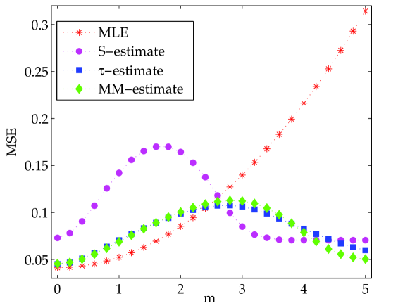
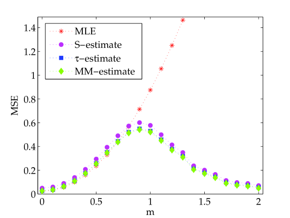
References

  • [1] Agullรณ J., Croux C., Van Aelst S. (2008). The Multivariate Least Trimmed Squares Estimator. Journal of Multivariate Analysis, 99, pp. 311 โ€“ 338.
  • [2] Bai Z., Chen X., Wu Y. (2008). On constrained M-estimation and its recursive analog in multivariate linear regression models. Statistica Sinica, 18, pp. 405โ€“424.
  • [3] Berrendero J., Mendes B., Tyler D. (2007). On the maximum bias functions of MM-estimates and constrained M-estimates of regression. The Annals of Statistics, 35, pp. 13 โ€“ 40.
  • [4] Bhatia R. (1952). Matrix Analysis. Springer.
  • [5] Bilodeau M., Duchesne P. (2000). Robust estimation of the SUR model. Canad. J. Statist., 28, pp. 227โ€“288.
  • [6] Croux C., Rousseeuw P., Hรถssjer O. (1994). Generalized Sโ€“estimators. Journal of the American Statistical Association 89, pp. 1271โ€“1281.
  • [7] Davies P. (1987). Asymptotic behavior of S-estimates of multivariate location parameters and dispersion matrices. Ann. Statist., 15, pp. 1269โ€“1292.
  • [8] Garcรญa Ben M. G., Martinez E., Yohai V. J. (2006). Robust estimation for the multivariate linear model based on a ฯ„๐œ\tau-scale. Journal of Multivariate Analysis, 97, pp. 1600โ€“1622.
  • [9] Hampel F. R. (1974). The influence curve and its role in robust estimation, J. Amer. Statist. Assoc., 69, pp. 383โ€“393.
  • [10] Huber P. J. (1964). Robust Estimation of a Location Parameter, The Annals of Mathematical Statistics, Vol. 35, No. 1, pp. 73โ€“101.
  • [11] Huber P. J. (1981). Robust Statistics, Wiley, New York.
  • [12] Janssens K., Deraedt I., Freddy A., Veekman J. (1998). Composition of 15โˆ’17tโ€‹h15superscript17๐‘กโ„Ž15-17^{th} century archeological glass vessels excavated in Antwerp, Belgium. Mikrochimica Acta,15 (Suppl.), 253โ€“267.
  • [13] Kent J., Tyler D. (1996). Constrained M-estimation for multivariate location and scatter. Ann Statist. 24, pp. 1346โ€“1370.
  • [14] Koenker P., Portnoy S. (1990). M-estimation of multivariate regressions. J. Amer. Statist. Assoc. 85, pp. 1060โ€“1068.
  • [15] Lopuhaรค H. (1992). Highly efficient estimators of multivariate location with high breakdown point. Ann. Statist. 20, pp. 398โ€“413.
  • [16] Maronna R. A., Martin R. D., Yohai V. J. (2006). Robust Statistics: Theory and Methods, John Wiley and Sons, New York.
  • [17] Mendes B., Tyler D. (1996). Constrained M-estimation for regression. In Robust Statistics, Data Analysis and Computer Intensive Methods. Lecture Notes in Statist. 109, H. Rieder, ed., Springer-Verlag, pp. 299โ€“320.
  • [18] Pakes A., Pollard D. (1989). Simulation and the asymptotics of optimization estimators. Econometrica. Vol. 57, No. 5, pp. 1027โ€“1057.
  • [19] Ranga Rao R. (1962). Relations between weak and uniform convergence of measures with applications. Ann. Math. Statist. 33, pp. 659โ€“680.
  • [20] Roelandt E., Van Aelst S., Croux C. (2009). Multivariate Generalized S-estimators, J. Multivar. Anal. 100, 5, pp. 876โ€“887.
  • [21] Rousseeuw P. (1985). Multivariate estimators with high breakdown point. W. Grossman, G. Pflug, I. Vincza, W. Wertz (Eds.), Mathematical Statistics and its Applications, vol. B, Reidel, Dordrecht, The Netherlands, pp. 283โ€“297.
  • [22] Rousseeuw P., Van Driessen K., Van Aelst S., Agullรณ J. (2004). Robust multivariate regression. Technometrics 46, pp. 293โ€“305.
  • [23] Salibiรกn-Barrera M., Van Aelst S., and Willems G. (2006). PCA based on Multivariate MM-estimators with Fast and Robust Bootstrap. Journal of the American Statistical Association, 101, pp. 1198โ€“1211.
  • [24] Seber G.A.F. (2007). A Matrix Handbook for Statisticians. John Wiley &\& Sons, Inc.
  • [25] Tatsuoka K. S., and Tyler D. E. (2000), The Uniqueness of S and M-Functionals Under Non-Elliptical Distributions, The Annals of Statistics, 28, pp. 1219โ€“1243.
  • [26] Van Aelst S., Willems G. (2005). Multivariate regression S-estimators for robust estimation and inference. Statist. Sinica 15, pp. 981โ€“1001
  • [27] Yohai V. (1987). High Breakdown-point and high efficiency robust estimates for regression. The Annals of Statistics, Vol. 15, No. 2., pp. 642โ€“656.