Existence and Properties
of Minimum Action Curves
for Degenerate Finsler Metrics

Abstract

We study a class of action functionals $S(\gamma)=\int_{\gamma}\ell(z,dz)$ on the space of unparameterized oriented rectifiable curves $\gamma$ in $\mathbb{R}^{n}$. The local action $\ell(x,y)$ is a degenerate type of Finsler metric that may vanish in certain directions $y\neq 0$, thus allowing for curves with positive Euclidean length but zero action. Given two sets $A_{1},A_{2}\subset\mathbb{R}^{n}$, we develop criteria under which $\exists\gamma^{\star}\in\Gamma_{A_{1}}^{A_{2}}:=\{\gamma\,|\,\gamma\text{ starts in }A_{1}\text{ and ends in }A_{2}\}$ such that $S(\gamma^{\star})=\inf\!\big{\{}S(\gamma)\,|\,\gamma\in\Gamma_{A_{1}}^{A_{2}}\big{\}}$. We then study the properties of these minimizers $\gamma^{\star}$, and we prove the non-existence of minimizers in some situations. Applied to a geometric reformulation of the quasipotential of large deviation theory, our results can prove the existence and properties of maximum likelihood transition curves between two metastable states in a stochastic process with small noise.

In memory of my beloved grandfather.
Julius Salzmann
${}^{\text{\textborn}}$ 11/03/1908  ~  ✝ 07/01/2009

Part I Results

1 Introduction

Geometric Action Functionals.

A geometric action $S$ is a mapping that assigns to every unparameterized oriented rectifiable curve $\gamma$ in $\mathbb{R}^{n}$ a number $S(\gamma)\in[0,\infty)$. It is defined via a curve integral

$$S(\gamma):=\int_{\gamma}\ell(z,dz):=\int_{0}^{1}\ell(\varphi,\varphi^{\prime})\,d\alpha,$$ (1.1)

where $\varphi\colon[0,1]\to\mathbb{R}^{n}$ is any absolutely continuous parameterization of $\gamma$, and where the local action $\ell\in C(\mathbb{R}^{n}\times\mathbb{R}^{n},[0,\infty))$ must have the properties

$$(i)\ \ \forall x,y\in\mathbb{R}^{n}\ \,\forall c\geq 0\colon\ \ \ell(x,cy)=c\ell(x,y),$$

$$(ii)\ \ x\in\mathbb{R}^{n} \ell(x,\cdot\,)$$ for every fixed the function is convex.

While (i) guarantees that the second integral in (1.1) is independent of the choice of $\varphi$, (ii) is necessary to ensure that $S$ is lower semi-continuous in a certain sense. A trivial example is given by $\ell(x,y)=|y|$, in which case $S(\gamma)$ is just the Euclidean length of $\gamma$, or more generally, by $\ell(x,y)=|y|_{g_{x}}$ for any Riemannian metric $g$. In fact, $\ell$ generalizes the well-studied notion of a Finsler metric [1] in that (a) $\ell$ only needs to be continuous (no smoothness required), and more importantly (b) $\ell^{2}$ need not be strictly convex.

Now given two sets $A_{1},A_{2}\subset\mathbb{R}^{n}$, in this work we develop criteria under which there exists a minimum action curve $\gamma^{\star}$ leading from $A_{1}$ to $A_{2}$, i.e. under which $\exists\gamma^{\star}\in\Gamma_{A_{1}}^{A_{2}}:=\{\gamma\,|\,\gamma\text{ starts in }A_{1}\text{ and ends in }A_{2}\}$ such that

$$S(\gamma^{\star})=\inf_{\begin{subarray}{c}\gamma\in\Gamma_{A_{1}}^{A_{2}}\end{subarray}}S(\gamma).$$ (1.2)

We then prove properties of the minimizer $\gamma^{\star}$ without knowing it explicitly.

Although our existence results can certainly be applied to the exemplary local actions given above, the present work was primarily motivated by a recently emerging problem from large deviation theory that is adding a considerable layer of difficulty: In contrast to usual Finsler metrics, in this example $\ell(x,y)$ vanishes in some direction $y=b(x)\neq 0$, which allows for curves $\gamma$ (the flowlines of the vector field $b$) with positive Euclidean length but vanishing action $S(\gamma)$.

Figure 1: Rare noise-induced transitions from one meta-stable state to another (green curve) stay with high probability near the minimum action curve $\gamma^{\star}$ (red).

Example: Large Deviation Theory.

Consider for some $b\in C^{1}(\mathbb{R}^{n},\mathbb{R}^{n})$ and small $\varepsilon>0$ the stochastic differential equation (SDE)

$$dX_{t}^{\varepsilon}=b(X_{t}^{\varepsilon})\,dt+\sqrt{\varepsilon}\,dW_{t},\qquad X_{0}^{\varepsilon}=x_{1},$$ (1.3)

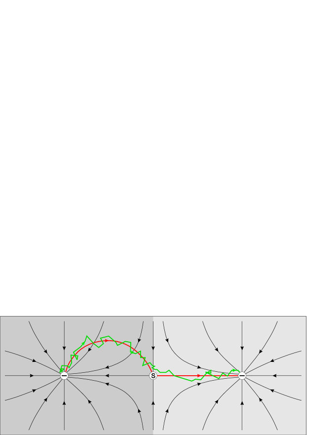
where $(W_{t})_{t\geq 0}$ is a Brownian motion, and where the zero-noise-limit, i.e. the ODE $\dot{x}=b(x)$, has two stable equilibrium points $x_{1},x_{2}\in\mathbb{R}^{n}$. The presence of small noise allows for rare transitions from $x_{1}$ to $x_{2}$ that would be impossible without the noise (green curve in Fig. 1), and one is interested in the frequency and the most likely path of these transitions. Both questions are answered within the framework of large deviation theory [2, 3], the key object being the quasipotential

$$V(x_{1},x_{2}) =\inf_{\begin{subarray}{c}T>0\\ \chi\in\bar{C}_{x_{1}}^{x_{2}}(0,T)\end{subarray}}S_{T}(\chi),$$ (1.4)

$$\text{where}\hskip 39.83368ptS_{T}(\chi) =\frac{1}{2}\int_{0}^{T}|b(\chi)-\dot{\chi}|^{2}\,dt,\hskip 39.83368pt$$ (1.5)

and where $\bar{C}_{x_{1}}^{x_{2}}(0,T)$ denotes the space of all absolutely continuous functions $\chi\colon[0,T]\to\mathbb{R}^{n}$ fulfilling $\chi(0)=x_{1}$ and $\chi(T)=x_{2}$.

An unpleasant feature of this formulation is that the minimization problem (1.4) does not have a minimizer $(T^{\star},\chi^{\star})$, the main reason being that by [2, Lemma 3.1] $\dot{\chi}^{\star}$ would need to vanish at $x_{1}$ and $x_{2}$, and typically also at some critical point along the way, and so $T^{\star}$ would have to be (doubly) infinite. This is a major problem for both analytical and numerical work, and so in [4, 5] the use of the alternative representation

$$V(x_{1},x_{2})=\inf_{\gamma\in\Gamma_{x_{1}}^{x_{2}}}S(\gamma)$$ (1.6)

was suggested, where the geometric action $S(\gamma)$ is given by

$$\hskip 91.04872pt\ell(x,y)=|b(x)||y|-{\langle b(x),y\rangle},\qquad\ \ \text{(SDE)}$$ (1.7)

which can be seen as a degenerate version of a Randers metric [1, Ch. 11]. The minimizer $\gamma^{\star}$ of (1.6), i.e. the maximum likelihood transition curve (the red curve in Fig. 1), seems more feasable to exist in this formulation since the time parameterization has been eliminated from the problem.

This geometric reformulation of the quasipotential generalizes also to other types of stochastic dynamics such as SDEs with multiplicative noise or continuous-time Markov jump processes [4, 5], with modified (in the latter case not Randers-like) local action $\ell$. It was shown to effectively remove the numerical difficulties [4, 5, 6, 7], and our goal in this monograph is now to demonstrate also its analytical advantages.

Existence of Minimizers; the Drift Vector Field.

Since minimizers $\gamma^{\star}$ of (1.2) have numerically been found to generally have cusps as they pass certain critical points (even in the basic case where $\ell$ is given by (1.7) with some smooth $b$, see Fig. 1 or e.g. [4, Fig. 4.1]), any a priori assumptions on the smoothness of $\gamma^{\star}$ in our existence proof would be counterproductive. This forbids the variational approach using the Euler-Lagrange equations associated to (1.2), and so instead we will opt for a lower semi-continuity argument.

A first result which is relatively easy to obtain is the following (Proposition 1): If there exists a minimizing sequence $(\gamma_{n})_{n\in\mathbb{N}}$ of (1.2) that is contained in some compact set $K\subset\mathbb{R}^{n}$ and has uniformly bounded curve lengths, then there exists a minimizer $\gamma^{\star}\in\Gamma_{A_{1}}^{A_{2}}$. In practice however, this criterion alone is of little use since minimizing sequences are not at our direct disposal and so their curve lengths can be hard to control. Instead, we would rather like to have criteria that are based on some explicitly available key ingredient of the local action $\ell$. What could this key ingredient be?

An essential property of (1.7) is that $\ell(x,y)$ vanishes whenever $y$ aligns with $b(x)$. In fact, such behavior is generic to large deviation geometric actions: For general stochastic dynamics, the drift vector field $b$ given by the zero-noise limit $\dot{x}=b(x)$ is the direction which the system can follow without the aid of the noise (as $\varepsilon\searrow 0$), and so any curve segment that follows a drift flowline has zero cost.

This observation complicates our existence proofs (which are based on Proposition 1) significantly, since it allows for long curves with vanishing or small action, and thus for minimizing sequences $(\gamma_{n})_{n\in\mathbb{N}}$ with unbounded curve lengths. For this reason, the flowline diagram of the drift vector field $b$ (or of a generalization thereof in the case of general geometric actions) will be the key object of our main criteria, Propositions 3 and 4.

Surprisingly, the drift $b$ is in fact all that these criteria depend on, while other aspects such as the nature of the noise in the case of large deviation geometric actions are largely irrelevant (except for the brute force estimate needed in Lemma 13). One may now argue that this indicates that our criteria may waste valuable information, potentially leaving us undecided where in fact a minimizer exists. However, we will give an example in which no minimizer exists and where the location that is responsible for this non-existence coincides exactly with the location where our criteria fail. This suggests that if our criteria fail, they do so for a reason.

Properties of Minimum Action Curves.

Then turning our attention to the properties of minimizers, we consider a subclass of geometric actions that still contains the large deviation geometric actions mentioned above. For our main result, suppose that the drift $b$ has two basins of attraction (see e.g. Figures 1, 6 (b) or 10), and let $\gamma^{\star}$ be the minimum action curve leading from one attractor to the other.

Since for the class of actions in question $\gamma^{\star}$ can follow the flowlines of $b$ at no cost, it is not surprising that the second (“downhill”) part of $\gamma^{\star}$ will be a flowline connecting a saddle point to the second attractor. In particular, the last hitting point of the separatrix is a point with zero drift (the saddle point). Here we prove also the non-obvious fact that also the first hitting point must have zero drift. In practice, such knowledge can be used either to gain confidence in the output of algorithms that compute $\gamma^{\star}$ numerically (such as the geometric minimum action method, gMAM, see [4, 5]), or to speed up such algorithms by restricting their search to only those curves with these properties.

Finally, we will demonstrate how the same result (Corollary 2) that is used to prove this property can also be used to prove the non-existence of minimizers is some situations.

The Structure of This Monograph.

This monograph is split into three parts: In Part I we lay out all our results on the existence of minimum action curves, we demonstrate on several examples how to use our criteria in practice, we discuss when minimizers do not exist, and finally we prove the above-mentioned properties of minimum action curves. The reader who is only interested in gaining enough working knowledge to use our existence criteria in practice will find it sufficient to read only this first part.

Part II contains essential proofs of a local existence property to which the global statement had been reduced in Part I. The reader who wants to know why the criteria in Part I work should also read this second part.

Part III contains the proof of a very technical lemma that is needed in the second part in order to deal with curves that are passing a saddle point. The reader can decide to skip this part without losing much insight.

Notation.

For a point $x\in\mathbb{R}^{n}$ and a radius $r>0$ we define the open and the closed balls

$$B_{r}(x):=\big{\{}w\in\mathbb{R}^{n}\,\big{|}\,|w-x|<r\big{\}}\qquad\text{\!and\!}\qquad\bar{B}_{r}(x):=\big{\{}w\in\mathbb{R}^{n}\,\big{|}\,|w-x|\leq r\big{\}}.$$

Similarly, for a set $A\subset\mathbb{R}^{n}$ and a distance $r>0$ we define the open and the closed neighborhoods $N_{r}(A)$ and $\bar{N}_{r}(A)$ as

$$N_{r}(A)\!:=\!\big{\{}w\in\mathbb{R}^{n}\,\big{|}\operatorname*{dist}(w,A)<r\big{\}}\;\;\text{and}\,\;\bar{N}_{r}(A)\!:=\!\big{\{}w\in\mathbb{R}^{n}\,\big{|}\operatorname*{dist}(w,A)\leq r\big{\}}.$$

Furthermore, we denote by $\bar{A}$ the closure of $A$ in $\mathbb{R}^{n}$, and by $A^{c}:=\mathbb{R}^{n}\setminus A$, $A^{\circ}:=(\overline{A^{c}})^{c}$ and $\partial A:=\bar{A}\setminus A^{\circ}$ the complement, the interior and the boundary of $A$ in $\mathbb{R}^{n}$, respectively. For a point $x$ on a $C^{1}$-manifold $M$ we denote by $T_{x}M$ the tangent space of $M$ at $x$.

For a function $f$ and a subset $A$ of its domain we denote by $f|_{A}$ the restriction of $f$ to $A$, and we use notation such as $f\equiv c$ to emphasize that $f$ is constant. Expressions of the form $\mathds{1}_{\textit{cond}}$ denote the indicator function that returns the value $1$ whenever the condition $cond$ is fulfilled and $0$ otherwise.

Finally, throughout the entire paper we let $\tilde{D}\subseteq D\subseteq\mathbb{R}^{n}$ be two fixed connected sets, where $D$ is open, and where $\tilde{D}$ is closed in $D$. An additional technical assumption on $\tilde{D}$ will be made at the beginning of Section 3.1. $D$ will serve as our state space, i.e. as the set that the curves $\gamma$ live in, and $\tilde{D}$ will be used for an additional constraint in our minimization, i.e. we will in fact minimize over $\Gamma_{A_{1}}^{A_{2}}:=\{\gamma\subset\tilde{D}\,|\,\gamma\text{ starts in }A_{1}\text{ and ends in }A_{2}\}$. (For simplicity we suppress the dependence of $\Gamma_{A_{1}}^{A_{2}}$ on $\tilde{D}$ in our notation.) If no such constraint is desired, just choose $\tilde{D}:=D$. The reader is encouraged to consider this simple unconstrained case $\tilde{D}=D$ whenever on first reading he may feel overwhelmed by some definition or statement involving $\tilde{D}$.

Acknowledgments.

The work of M. Heymann is partially supported by the National Science Foundation via grant DMS-0616710. I want to thank Weinan E, Gerard Ben Arous, Eric Vanden-Eijnden, Lenny Ng, Marcus Werner and Stephanos Venakides for some useful suggestions and comments. I also want to thank the Duke University Mathematics Department and in particular Jonathan Mattingly and Mike Reed for providing me with the inspiring environment and the freedom without which this work would not have been possible.

2 Geometric Action Functionals

2.1 Rectifiable Curves and Absolutely Continuous Functions

An unparameterized oriented curve $\gamma$ is an equivalence class of functions$\varphi\in C([0,T],D)$,  $T>0$, that are identical up to continuous non-decreasing changes of their parameterizations, or more formally, whose Fréchet distance to each other vanishes. In this paper we will tacitly assume that all our curves are unparameterized and oriented.

A curve $\gamma$ is called rectifiable [8, p.115] if for some (and thus for every) parameterization $\varphi\in C([0,T],D)$ of $\gamma$ we have

$$\operatorname*{length}(\gamma):=\operatorname*{length}(\varphi):=\sup_{\begin{subarray}{c}N\in\mathbb{N}\\ 0=t_{0}<\dots<t_{N}=T\end{subarray}}\,\sum_{i=1}^{N}\big{|}\varphi(t_{i})-\varphi(t_{i-1})\big{|}<\infty.$$

It is easy to see that $\operatorname*{length}(\varphi)$ is in fact the same for any parameterization $\varphi$ of $\gamma$, and that it is finite if and only if all the component functions of $\varphi$ are of bounded variation [8, Thm. 3.1]. We will denote the set of rectifiable curves by $\Gamma$.

A function $\varphi\colon[0,T]\to D$ is said to be absolutely continuous [8, p.127] if for every $\varepsilon>0$ there exists a $\delta>0$ such that for any finite collection of disjoint intervals $[t_{i-1},t_{i})\subset[0,T]$, $i=1,\dots,N$, we have

$$\sum_{i=1}^{N}(t_{i}-t_{i-1})<\delta\qquad\Longrightarrow\qquad\sum_{i=1}^{N}\big{|}\varphi(t_{i})-\varphi(t_{i-1})\big{|}<\varepsilon.$$

We will denote the space of absolutely continuous functions with values in our fixed set $D$ by $\bar{C}({0,T})$. One can show [8, Prop. 1.12(ii) and Thm. 3.11] that a function $\varphi$ is in $\bar{C}({0,T})$ if and only if there exists an $L^{1}$-function which we denote by $\varphi^{\prime}$ such that $\varphi(t)=\varphi(0)+\int_{0}^{t}\varphi^{\prime}(\tau)\,d\tau$ for $\forall t\in[0,T]$. In that case, $\varphi$ is differentiable in the classical sense at almost every $t\in[0,T]$, with derivative $\varphi^{\prime}(t)$.

Clearly, every function $\varphi\in\bar{C}({0,T})$ describes a rectifiable curve $\gamma$ since for every partition $0=t_{0}<\cdots<t_{N}=T$ we have

$$\sum_{i=1}^{N}\big{|}\varphi(t_{i})-\varphi(t_{i-1})\big{|}=\sum_{i=1}^{N}\bigg{|}\int_{t_{i}}^{t_{i-1}}\varphi^{\prime}\,dt\bigg{|}\leq\int_{0}^{T}|\varphi^{\prime}|\,dt<\infty,$$

and it is not hard to show [8, Thm. 4.1] that $\operatorname*{length}(\gamma)=\int_{0}^{T}|\varphi^{\prime}|\,dt$. The reverse is not true: Not every function $\varphi$ that describes a rectifiable curve $\gamma\in\Gamma$ is necessarily absolutely continuous (a counterexample can be constructed using the Cantor function [8, p.125]). However, we have the following:

Lemma 1 (Parameterization by arclength).

(i) Any curve $\gamma\in\Gamma$ can be parameterized by a unique function $\varphi_{\gamma}\in\bar{C}({0,1})$ with $|\varphi_{\gamma}^{\prime}|\equiv\operatorname*{length}(\gamma)$ a.e..
(ii) If $\varphi\in\bar{C}({0,T})$ is any absolutely continuous parameterization of $\gamma$ then $\varphi=\varphi_{\gamma}\circ\beta$ for some absolutely continuous function $\beta\colon[0,T]\to[0,1]$, and we have $\varphi^{\prime}=(\varphi_{\gamma}^{\prime}\circ\beta)\cdot\beta^{\prime}$ and $\beta^{\prime}\geq 0$ a.e. on $[0,1]$.

Proof.

(i) This is a trivial modification of [8, p.136].
(ii) In the proof in [8, p.136] it is shown that for any parameterization $\varphi\in C([0,T],D)$ of $\gamma$ the function $\varphi_{\gamma}$ fulfills $\varphi(t)=\varphi_{\gamma}(\beta(t))$ for $\forall t\in[0,T]$, where $\beta\colon[0,T]\to[0,1]$ is defined by $\beta(t):=\operatorname*{length}\!\big{(}\varphi|_{[0,t]}\big{)}/\operatorname*{length}(\gamma)$. For any collection of disjoint intervals $[t_{i-1},t_{i})\subset[0,T]$, $i=1,\dots,N$, we have

$$\sum_{i=1}^{N}\big{(}\beta(t_{i})-\beta(t_{i-1})\big{)} =\frac{1}{\operatorname*{length}(\gamma)}\sum_{i=1}^{N}\operatorname*{length}\!\big{(}\varphi|_{[t_{i-1},t_{i}]}\big{)}$$

$$=\frac{1}{\operatorname*{length}(\gamma)}\sum_{i=1}^{N}\,\sup_{\begin{subarray}{c}M_{i}\in\mathbb{N}\\ t_{i-1}=s_{0}^{i}<\dots<s_{M_{i}}^{i}=t_{i}\end{subarray}}\,\sum_{k=1}^{M_{i}}\big{|}\varphi(s_{k}^{i})-\varphi(s_{k-1}^{i})\big{|}$$

$$=\frac{1}{\operatorname*{length}(\gamma)}\!\sup_{\begin{subarray}{c}M_{1}\in\mathbb{N}\\ t_{0}=s_{0}^{1}<\dots<s_{M_{1}}^{1}=t_{1}\end{subarray}}\cdots\sup_{\begin{subarray}{c}M_{N}\in\mathbb{N}\\ t_{N-1}=s_{0}^{N}<\dots<s_{M_{N}}^{N}=t_{N}\end{subarray}}\sum_{i=1}^{N}\sum_{k=1}^{M_{i}}\big{|}\varphi(s_{k}^{i})-\varphi(s_{k-1}^{i})\big{|},$$

and since for $\varphi\in\bar{C}({0,T})$ the last double sum can be made arbitrarily small by ensuring that $\sum_{i=1}^{N}\sum_{k=1}^{M_{i}}(s_{k}^{i}-s_{k-1}^{i})=\sum_{i=1}^{N}(t_{i}-t_{i-1})$ is sufficiently small, this shows that $\beta$ is absolutely continuous. Clearly, $\beta^{\prime}\geq 0$ a.e. since $\beta$ is non-decreasing, and for $\forall t\in[0,T]$ we have

$$\int_{0}^{t}\varphi^{\prime}\,d\tau =\varphi(t)-\varphi(0)=\varphi_{\gamma}(\beta(t))-\varphi_{\gamma}(\beta(0))$$

$$=\int_{\beta(0)}^{\beta(t)}\varphi_{\gamma}^{\prime}\,d\alpha=\int_{0}^{t}\varphi_{\gamma}^{\prime}(\beta(\tau))\beta^{\prime}(\tau)\,d\tau$$

(for the last step, see [8, p.149, Ex.21]), which implies that $\varphi^{\prime}=(\varphi_{\gamma}^{\prime}\circ\beta)\cdot\beta^{\prime}$ a.e. on $[0,T]$. ∎

The following lemma is a result on the uniform convergence of absolutely continuous functions. We will use the notation $\varphi\subset G$ (for a function $\varphi\in\bar{C}({0,1})$ and a set $G\subset\mathbb{R}^{n}$) to indicate that $\varphi(\alpha)\in G$ for $\forall\alpha\in[0,1]$. Similarly, for a curve $\gamma\in\Gamma$ we write $\gamma\subset G$ to indicate that $\varphi_{\gamma}\subset G$.

Lemma 2.

(i) If a sequence $(\varphi_{n})_{n\in\mathbb{N}}\subset\bar{C}({0,1})$ fulfills $\varphi_{n}\subset K$ for $\forall n\in\mathbb{N}$ and some compact set $K\subset D$, and if

$$M:=\sup_{n\in\mathbb{N}}\ \operatorname*{ess\,sup}_{\alpha\in[0,1]}|\varphi_{n}^{\prime}(\alpha)|<\infty,$$ (2.1)

then there exists a uniformly converging subsequence.
(ii) If a sequence $(\varphi_{n})_{n\in\mathbb{N}}\subset\bar{C}({0,1})$ fulfilling the conditions of part (i) converges uniformly then its limit $\varphi$ is in $\bar{C}({0,1})$ and fulfills $|\varphi^{\prime}|\leq M$ a.e..

Proof.

(i) The sequence $(\varphi_{n})_{n\in\mathbb{N}}$ is equicontinuous since by (2.1) we have

$$|\varphi_{n}(\alpha_{1})-\varphi_{n}(\alpha_{0})|=\bigg{|}\int_{\alpha_{0}}^{\alpha_{1}}\varphi_{n}^{\prime}\,d\alpha\bigg{|}\leq\int_{\alpha_{0}}^{\alpha_{1}}|\varphi_{n}^{\prime}|\,d\alpha\leq M(\alpha_{1}-\alpha_{0})$$

for $\alpha_{0}<\alpha_{1}$ and $\forall n\in\mathbb{N}$, and so we can apply the Arzelà-Ascoli theorem.
(ii) By the same estimate, for any collection of disjoint intervals $[\alpha_{i-1},\alpha_{i})$ $\subset[0,1]$, $i=1,\dots,N$, we have

$$\sum_{i=1}^{N}\big{|}\varphi(\alpha_{i})-\varphi(\alpha_{i-1})\big{|} =\lim_{n\to\infty}\sum_{i=1}^{N}\big{|}\varphi_{n}(\alpha_{i})-\varphi_{n}(\alpha_{i-1})\big{|}\leq M\sum_{i=1}^{N}(\alpha_{i}-\alpha_{i-1}).$$

This shows that $\varphi$ is absolutely continuous, and (taking $N=1$ and recalling that $\varphi^{\prime}$ is the classical derivative a.e.) that $|\varphi^{\prime}|\leq M$ a.e.. Since $K$ is compact and $\varphi_{n}\subset K$ for $\forall n\in\mathbb{N}$, we have $\varphi\subset K\subset D$ and thus $\varphi\in\bar{C}({0,1})$. ∎

Curves that pass points in infinite length.

Sometimes we will have to work with curves that do not have finite length (i.e. that are not rectifiable). We denote by $\tilde{C}(0,1)\supset\bar{C}({0,1})$ the space of all functions in $C([0,1],D)$ that are absolutely continuous in neighborhoods of all but at most finitely many $\alpha_{i}\in[0,1]$, and we denote by $\tilde{\Gamma}\supset\Gamma$ the set of all curves that can be parameterized by a function $\varphi\in\tilde{C}(0,1)$.

Note that for $\forall\varphi\in\tilde{C}(0,1)$, $\varphi^{\prime}$ is still defined a.e., but one can see that for these exceptional values $\alpha_{i}$ we have $\int_{[0,1]\cap[\alpha_{i}-\varepsilon,\alpha_{i}+\varepsilon]}|\varphi^{\prime}|\,d\alpha=\infty$ for $\forall\varepsilon>0$. We therefore say that the curve $\gamma\in\tilde{\Gamma}$ given by $\varphi$ “passes the points $\varphi(\alpha_{i})$ in infinite length.”

Of particular use in our work is, for fixed $x\in D$, the set $\tilde{\Gamma}(x)$ of all curves that are either of finite length (i.e. rectifiable) or that pass $x$ once in infinite length (note that $\Gamma\subset\tilde{\Gamma}(x)\subset\tilde{\Gamma}$). More precisely, these are the curves that can be parameterized by functions in the set $\tilde{C}(x)$, which we define to be the set of functions $\varphi\in C([0,1],D)$ such that
    either $\varphi\in\bar{C}({0,1})$, or $\varphi(\tfrac{1}{2})=x$, and $\varphi|_{[0,1/2-a]}$ and $\varphi|_{[1/2+a,1]}$ are abs. cont. for $\forall a\in(0,\tfrac{1}{2})$.
See the end of this section and Fig. 2 for an illustration of these classes of curves.
In preparation for Lemma 3, which is the equivalent of Lemma 2 for sequences of functions in $\tilde{C}(x)$, we introduce the following notation: For a curve $\gamma$ and a point $x$ we say that $\gamma$ passes $x$ at most once if for any parameterization $\varphi\in C([0,1])$ of $\gamma$ we have

$$\big{(}\exists 0\leq\alpha_{1}<\alpha_{2}\leq 1\colon\ \varphi(\alpha_{1})=\varphi(\alpha_{2})=x\big{)}\quad\Rightarrow\quad\forall\alpha\in[\alpha_{1},\alpha_{2}]\colon\ \varphi(\alpha)=x.$$ (2.2)

For a Borel set $E\subset D$ and a curve $\gamma\in\tilde{\Gamma}$ we define

$$\operatorname*{length}(\gamma|_{E}):=\int_{\gamma}\mathds{1}_{z\in E}\,|dz|=\int_{0}^{1}|\varphi^{\prime}|\mathds{1}_{\varphi\in E}\,d\alpha\ \in[0,\infty]$$

for any parameterization $\varphi\in\tilde{C}(0,1)$ of $\gamma$.

Lemma 3.

Let $x\in D$, let the sequence $(\gamma_{n})_{n\in\mathbb{N}}\subset\tilde{\Gamma}(x)$ fulfill $\gamma_{n}\subset K$ for $\forall n\in\mathbb{N}$ and some compact set $K\subset D$, suppose that every curve $\gamma_{n}$ passes $x$ at most once, and suppose that there exists a function $\eta\colon(0,\infty)\to[0,\infty)$ such that

$$\forall n\in\mathbb{N}\ \,\forall u>0:\ \ \operatorname*{length}\!\big{(}\gamma_{n}|_{\bar{B}_{u}(x)^{c}}\big{)}\leq\eta(u).$$ (2.3)

Then there exist parameterizations $\varphi_{n}\in\tilde{C}(x)$ of the curves $\gamma_{n}$ such that a subsequence $(\varphi_{n_{k}})_{k\in\mathbb{N}}$ converges pointwise on $[0,1]$ and uniformly on the sets $[0,\frac{1}{2}-a]\cup[\frac{1}{2}+a,1]$, $a\in(0,\frac{1}{2})$. The limit $\varphi$ is in $\tilde{C}(x)$, and the corresponding curve $\gamma\in\tilde{\Gamma}(x)$ fulfills

$$\hskip 33.57404pt\forall u>0\colon\ \operatorname*{length}\!\big{(}\gamma|_{\bar{B}_{u}(x)^{c}}\big{)}\leq\eta(u).$$ (2.4)

Proof.

See Appendix A.1. This proof uses Lemma 5 (i). ∎

Introducing some final notation, for two sets $A_{1},A_{2}\subset\tilde{D}$ we write

$$\Gamma_{A_{1}}^{A_{2}} :=\big{\{}\gamma\in\Gamma\,\big{|}\,\text{$\gamma\subset\tilde{D}$, $\gamma$ starts in $A_{1}$ and ends in $A_{2}$}\big{\}},$$

$$\bar{C}_{A_{1}}^{A_{2}}(0,1) :=\big{\{}\varphi\in\bar{C}({0,1})\,\big{|}\,\varphi\subset\tilde{D},\ \varphi(0)\in A_{1},\ \varphi(1)\in A_{2}\big{\}},$$

and for two points $x_{1},x_{2}\in\tilde{D}$ we similarly define $\Gamma_{x_{1}}^{x_{2}}$ and $\bar{C}_{x_{1}}^{x_{2}}(0,1)$. The sets $\tilde{\Gamma}_{A_{1}}^{A_{2}}$, $\tilde{C}_{A_{1}}^{A_{2}}(0,1)$, $\tilde{\Gamma}_{x_{1}}^{x_{2}}$, $\tilde{C}_{x_{1}}^{x_{2}}(0,1)$, $\tilde{\Gamma}_{x_{1}}^{x_{2}}(x)$ and $\tilde{C}_{x_{1}}^{x_{2}}(x)$ are defined analogously.

Figure 2: Illustration of the various classes of curves.

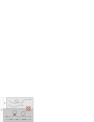
Summary of the various classes of curves (see Fig. 2).

All curves are unparameterized and oriented, and they may have loops and cusps. The class $\Gamma$ contains only curves with finite length, while curves in $\tilde{\Gamma}\supset\Gamma$ may reach and/or leave finitely many points in infinite length, also repeatedly. For some fixed $x\in D$ (marked by the cross), $\tilde{\Gamma}(x)$ contains all of $\Gamma$, plus all the curves that pass $x$ once in infinite length; they cannot pass any other point in infinite length, and they cannot pass $x$ twice in infinite length. The sub- and superscripts $x_{1}$ and $x_{2}$ or $A_{1}$ and $A_{2}$ add constraints to the start and end points of these functions and curves and require them to take values in $\tilde{D}$.

2.2 The Class $\mathcal{G}$ of Geometric Actions, Drift Vector Fields

In this section we will define the class $\mathcal{G}$ of geometric action functionals, and we will generalize the concept of a “drift vector field” $b(x)$ from the large deviation geometric action of the SDE (1.3), given by (1.7), to general geometric actions $S\in\mathcal{G}$.

Definition 1.

We denote by $\mathcal{G}$ the set of all functionals $S\colon\tilde{\Gamma}\to[0,\infty]$ of the form

$$S(\gamma):=\int_{\gamma}\ell(z,dz):=\int_{0}^{1}\ell(\varphi,\varphi^{\prime})\,d\alpha,$$ (2.5)

where $\varphi\in\tilde{C}(0,1)$ is an arbitrary parameterization of $\gamma$, and where the local action $\ell\in C(D\times\mathbb{R}^{n},[0,\infty))$ has the following properties:
(i) $\forall x\in D\ \,\forall y\in\mathbb{R}^{n}\ \,\forall c\geq 0\colon\ \ \ell(x,cy)=c\ell(x,y)$, (ii) for every fixed $x\in D$ the function $\ell(x,\cdot\,)$ is convex.
For $\varphi\in\tilde{C}(0,1)$ we will sometimes use the notation $S(\varphi):=\int_{0}^{1}\ell(\varphi,\varphi^{\prime})\,d\alpha$, and for any interval $[\alpha_{1},\alpha_{2}]\subset[0,1]$ we will denote by $S(\varphi|_{[\alpha_{1},\alpha_{2}]}):=$$\int_{\alpha_{1}}^{\alpha_{2}}\ell(\varphi,\varphi^{\prime})\,d\alpha$ the action of the curve segment parameterized by $\varphi|_{[\alpha_{1},\alpha_{2}]}$.

As we will see next, (i) is needed to show that (2.5) is independent of the specific choice of $\varphi$, while (ii) is essential to show that $S$ is lower semi-continuous in a certain sense (Lemma 5). Observe also that (i) implies that $\ell(x,0)=0$ for $\forall x\in D$.

Lemma 4.

Functionals $S\in\mathcal{G}$ and their local actions $\ell(x,y)$ have the following properties:
​​​(i) $S(\gamma)$ is well-defined, i.e. (2.5) is independent of the specific choice of $\varphi$. ​​​(ii) For  $\forall\!$ compact $K\subset D\ \,\exists c_{1}\!=\!c_{1}(K)\!>\!0\ \,\forall x\in K\ \,\forall y\in\mathbb{R}^{n}\colon\,\ell(x,y)\!\leq\!c_{1}|y|$. In particular, we have for $\forall\gamma\in\tilde{\Gamma}$ with $\gamma\subset K\colon$ $S(\gamma)\leq c_{1}\cdot\operatorname*{length}(\gamma)$.

Proof.

(i) Given a curve $\gamma\in\Gamma$ and any parameterization $\varphi\in\bar{C}({0,1})$ of $\gamma$, we use the representation $\varphi=\varphi_{\gamma}\circ\beta$ of Lemma 1 (ii) and Definition 1 (i) to find that

$$\int_{0}^{1}\ell(\varphi,\varphi^{\prime})\,d\alpha =\int_{0}^{1}\ell\big{(}\varphi_{\gamma}\circ\beta,(\varphi_{\gamma}^{\prime}\circ\beta)\beta^{\prime}\big{)}\,d\alpha$$

$$=\int_{0}^{1}\ell(\varphi_{\gamma}\circ\beta,\varphi_{\gamma}^{\prime}\circ\beta)\beta^{\prime}\,d\alpha=\int_{0}^{1}\ell(\varphi_{\gamma},\varphi_{\gamma}^{\prime})\,d\beta,$$

where the last step follows again from [8, p.149, Ex.21]. By the uniqueness of $\varphi_{\gamma}$, the right-hand side only depends on $\gamma$. The proof for general curves $\gamma\in\tilde{\Gamma}$ is based on the same calculation.

(ii) Given any $K$, set $c_{1}:=1+\max_{x\in K,|y|=1}\ell(x,y)>0$, use Definition 1 (i) to show that $\ell(x,y)=|y|\ell\big{(}x,\frac{y}{|y|}\big{)}\leq c_{1}|y|$ for $\forall y\neq 0$, and recall that $\ell(x,0)=0$. In particular, if $\varphi\in\tilde{C}(0,1)$ is a parameterization of some $\gamma\in\tilde{\Gamma}$ with $\gamma\subset K$ then $S(\gamma)=\int_{0}^{1}\ell(\varphi,\varphi^{\prime})\,d\alpha\leq c_{1}\int_{0}^{1}|\varphi^{\prime}|\,d\alpha=c_{1}\cdot\operatorname*{length}(\gamma)$. ∎

Lemma 5 (Lower semi-continuity).

For $\forall S\in\mathcal{G}$ we have the following:
​​​(i) If a sequence $(\varphi_{n})_{n\in\mathbb{N}}\subset\bar{C}({0,1})$ fulfilling (2.1) has a uniform limit $\varphi\in\bar{C}({0,1})$ then $\liminf_{n\to\infty}S(\varphi_{n})\geq S(\varphi)$. ​​​(ii) The limit $\gamma$ constructed in Lemma 3 fulfills $\liminf_{n\to\infty}S(\gamma_{n})\geq S(\gamma)$.

Proof.

See Appendix A.2. ∎

Definition 2.

Let $S\in\mathcal{G}$. A vector field $b\in C^{1}(D,\mathbb{R}^{n})$ is called a drift of $S$ if for $\forall\!$ compact $K\subset D$ $\exists c_{2}\!=\!c_{2}(K)>0\ \forall x\in K\ \forall y\in\mathbb{R}^{n}:$

$$\ell(x,y)\geq c_{2}\big{(}|b(x)||y|-{\langle b(x),y\rangle}\big{)}.$$ (2.6)

The right-hand side of (2.6) is a constant multiple of the local large deviation geometric action (1.7) of the SDE (1.3) with drift $b(x)$ and homogeneous noise, and thus we see that for the geometric action associated to (1.3), the vector field $b(x)$ in (1.3) is clearly a drift also in this generalized sense (take $c_{2}=1$). The inequality (2.6), which will only be used in the key estimate Lemma 26 and its weaker version Lemma 16, effectively reduces our proofs for an arbitrary action $S\in\mathcal{G}$ to the case of the action given by (1.7), and it is ultimately the reason why the conditions of our main criteria, Propositions 3 and 4, solely depend on the drift and not on any other aspect of the action $S$.

The drift vector field $b(x)$ in Definition 2 is not a uniquely defined object: If $b$ is a drift of some action $S\in\mathcal{G}$ and if $\beta\in C^{1}(D,[0,\infty))$ then $\beta\cdot b$ is a drift of $S$ as well (with modified constants $c_{2}$), and in particular the vector field $b(x)\equiv 0$ is a drift of any action $S\in\mathcal{G}$. Note however that (i) if $\beta(x)>0$ for $\forall x\in D$ then the vector fields $b$ and $\beta b$ have the same flowline diagrams, and we will find that our criteria will not distinguish between these two choices; (ii) if on the other hand $\beta(x)=0$ and $b(x)\neq 0$ for some $x\in D$ then the flowline diagrams of $b$ and $\beta\cdot b$ are different, and our criteria may only apply to $b$ but not to $\beta\cdot b$. In general, a good choice for the drift (i.e. one that lets us get the most out of our criteria) will be one with only as many roots as necessary.

Definition 3.

For a given vector field $b\in C^{1}(D,\mathbb{R}^{n})$ we define the flow $\psi\in C^{1}(D\times\mathbb{R},D)$ as the unique solution of the ODE

$$\begin{cases}\partial_{t}\psi(x,t)\hskip 1.42271pt=b(\psi(x,t))&\text{for}\quad x\in D,\ t\in\mathbb{R},\\ \hskip 9.24706pt\psi(x,0)=x&\text{for}\quad x\in D.\end{cases}$$ (2.7)

By a standard result from the theory of ODEs [10, §7.3, Corollary 4], our regularity assumption on $b$ implies that the solution $\psi(x,t)$ is well-defined locally (i.e. for small $t$), unique, and $C^{1}$ in $(x,t)$. However, since $b$ will always play the role of a drift, we may assume that $\psi(x,t)$ is in fact defined globally, i.e. for $\forall t\in\mathbb{R}$: Indeed, if this is not the case then we can instead consider the modified drift $\beta\cdot b$, for some function $\beta\in C^{1}(D,(0,\infty))$ that vanishes so fast near the boundary $\partial D$ that the associated flow $\tilde{\psi}$ only reaches $\partial D$ in infinite time (i.e. $\tilde{\psi}(x,t)$ is defined for $\forall(x,t)\in D\times\mathbb{R}$), and the only aspect of the flow that will be relevant to us (the flowline diagram) remains invariant under this change.

Finally, recall that under this additional assumption we have $\psi(\psi(x,t),s)$$=\psi(x,t+s)$ and $\partial_{t}\nabla\psi(x,t)=\nabla b(\psi(x,t))$ for $\forall x\in D$ and $\forall t,s\in\mathbb{R}$.
A special role in our theory will be played by so-called critical points.

Definition 4.

For a given $S\in\mathcal{G}$ with local action $\ell(x,y)$, a point $x\in D$ is called a critical point if  $\forall y\in\mathbb{R}^{n}\colon\ \ell(x,y)=0$.

2.3 The Subclass $\mathcal{H}$ of Hamiltonian Geometric Actions

We will now consider a particular way of constructing a geometric action from a Hamiltonian $H(x,\theta)$, which was introduced in [4] in the context of large deviation theory.

Lemma 6.

Let the Hamiltonian $H\in C(D\times\mathbb{R}^{n},\mathbb{R})$ fulfill the assumptions
​​(H1) $\forall x\in D\colon\ H(x,0)\leq 0$, ​​(H2) the derivatives $H_{\theta}$ and $H_{\theta\theta}$ exist and are continuous in $(x,\theta)$, ​​(H3) $\forall\!$ compact $K\!\subset\!D$ $\exists m_{K}\!\!>\!0$ $\forall x\!\in\!\!K$ $\forall\theta,\xi\!\in\!\mathbb{R}^{n}\colon{\langle\xi,H_{\theta\theta}(x,\theta)\xi\rangle}\geq m_{K}|\xi|^{2}$​.
Then the function $\ell\colon D\times\mathbb{R}^{n}\to[0,\infty)$ defined by

$$\ell(x,y):= \,\max\!\big{\{}{\langle y,\theta\rangle}\,\big{|}\,\theta\in\mathbb{R}^{n},\,H(x,\theta)\leq 0\big{\}}$$ (2.8a)

$$= \,\max\!\big{\{}{\langle y,\theta\rangle}\,\big{|}\,\theta\in\mathbb{R}^{n},\,H(x,\theta)=0\big{\}}$$ (2.8b)

has the properties of Definition 1, and so it defines a geometric action $S\in\mathcal{G}$.

Proof.

The sets $L_{x}:=\{\theta\in\mathbb{R}^{n}\,|\,H(x,\theta)\leq 0\}$ are bounded, in fact uniformly for all $x$ in any compact set $K\subset D$, since for $\forall x\in K\ \forall\theta\in L_{x}\ \exists\tilde{\theta}\in\mathbb{R}^{n}\colon$

$$0\geq H(x,\theta) =H(x,0)+{\langle H_{\theta}(x,0),\theta\rangle}+\tfrac{1}{2}{\big{\langle}\theta,H_{\theta\theta}(x,\tilde{\theta})\theta\big{\rangle}}$$

$$\geq-\max_{x\in K}|H(x,0)|-\max_{x\in K}|H_{\theta}(x,0)|\cdot|\theta|+\tfrac{1}{2}m_{K}|\theta|^{2}.$$ (2.9)

This shows that $\ell$ is finite-valued, and since $0\in L_{x}$ by (H1) we have $\ell(x,y)\geq{\langle y,0\rangle}=0$ for $\forall y\in\mathbb{R}^{n}$. The fact that the representations (2.8a) and (2.8b) are equivalent is obvious for $y=0$; for $y\neq 0$ observe that for $\forall\theta\in\mathbb{R}^{n}$ with $H(x,\theta)<0$ the boundedness of $L_{x}$ implies that there $\exists c>0$ such that $H(x,\theta+cy)=0$, and ${\langle y,\theta+cy\rangle}\geq{\langle y,\theta\rangle}$. The relation $\ell(x,cy)=c\ell(x,y)$ for $\forall c\geq 0$ is clear, and $\ell(x,\cdot\,)$ is convex as the supremum of linear functions. The continuity at any point $(x_{0},y_{0}=0)$ follows from the estimate $\ell(x,y)\leq M|y|$ for $\forall y\in\mathbb{R}^{n}$ and all $x$ in some ball $\bar{B}_{\varepsilon}(x_{0})\subset D$, where $M:=\sup\!\big{\{}|\theta|\,\big{|}\,\theta\in\bigcup_{x\in\bar{B}_{\varepsilon}(x_{0})}L_{x}\big{\}}$. The continuity everywhere else will follow from Lemma 8 (i).​ ∎

Definition 5.

(i) We denote the class of all Hamiltonian geometric actions, i.e. of all actions $S$ constructed as in Lemma 6, by $\mathcal{H}\subset\mathcal{G}$.
(ii) We denote by $\mathcal{H}_{0}\subset\mathcal{H}$ the class of all geometric actions $S\in\mathcal{H}$ that are constructed from a Hamiltonian $H$ which fulfills the stronger assumption
  (H1’)  $\forall x\in D\colon\ H(x,0)=0$.

Note that since $\ell$ depends on $H$ only through its $0$-level sets, different Hamiltonians $H$ can induce the same geometric action $S\in\mathcal{H}$. In particular, for $\forall\beta\in C(D,(0,\infty))$ the Hamiltonians $H(x,\theta)$ and $\beta(x)H(x,\theta)$ induce the same action $S$. The next lemma shows how Definition 4 can be expressed in terms of $H$, and that Assumption (H1’) does not depend on the choice of $H$.

Lemma 7.

Let $S\in\mathcal{H}$, and let $H$ be a Hamiltonian that induces $S$.
(i) A point $x\in D$ is critical if and only if

$$H_{\theta}(x,0)=0\qquad\text{and}\qquad H(x,0)=0,$$ (2.10)

and in that case (2.10) holds in fact for every Hamiltonian that induces $S$.
(ii) $\forall x\in D\colon\ \big{(}H(x,0)=0\ \Leftrightarrow\ \exists y\in\mathbb{R}^{n}\setminus\{0\}\colon\ \ell(x,y)=0\big{)}$. In particular, if some $H$ inducing $S$ fulfills (H1’) then all of them do.

Proof.

See Appendix A.3. For part (ii) see also Fig. 3 (b). ∎

To actually compute $\ell(x,y)$ from a given Hamiltonian $H$, and for many proofs, the following alternative representation of $\ell$ is oftentimes useful. It can be derived by carrying out the constraint maximization in (2.8b) with the method of Lagrange multipliers.

Lemma 8.

(i) For every fixed $x\in D$ and $y\in\mathbb{R}^{n}\setminus\{0\}$ the system

$$H_{\theta}(x,\vartheta)=\lambda y,\qquad H(x,\vartheta)=0,\qquad\lambda\geq 0$$ (2.11)

has a unique solution $(\vartheta(x,y),\lambda(x,y))$, the functions $\vartheta\colon D\times(\mathbb{R}^{n}\setminus\{0\})\to\mathbb{R}^{n}$ and $\lambda\colon D\times(\mathbb{R}^{n}\setminus\{0\})\to[0,\infty)$ are continuous, and the function $\ell$ defined in (2.8a) can be written as

$$\ell(x,y)=\begin{cases}{\langle y,\vartheta(x,y)\rangle}&\text{if }y\neq 0,\\ 0&\text{if }y=0.\end{cases}$$ (2.12)

(ii) If $S\in\mathcal{H}$ is induced by $H$ then a point $x\in D$ is critical if and only if $\exists y\neq 0\colon\ \lambda(x,y)=0$. In that case, we have in fact $\lambda(x,y)=0$ for $\forall y\neq 0$.

Proof.

See Appendix A.4. ∎

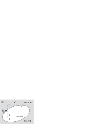
See Fig. 3 (a) for a geometric interpretation of (2.8a)-(2.8b) and (2.11)-(2.12): By Assumption (H3) the function $H(x,\cdot\,)$ and thus also its 0-sublevel set $\{\theta\in\mathbb{R}^{n}\,|\,H(x,\theta)\leq 0\}$ is strictly convex, and by Assumption (H1) it contains the origin. The maximizer in (2.8a), $\theta=\vartheta(x,y)$, is the unique point on its boundary where the outer normal aligns with $y$, and the local action $\ell(x,y)$ is $|y|$ times the component of $\vartheta(x,y)$ in the direction $y$.

Figure 3: (a) Illustration of (2.8a)-(2.8b) and (2.11)-(2.12), for fixed $x\in D$ and $y\in\mathbb{R}^{n}\setminus\{0\}$, in the case $H(x,0)<0$.  (b) If $H(x,0)=0$ and if $y$ aligns with $H_{\theta}(x,0)$ then we have $\vartheta=0$.

The following lemma provides a quick way to obtain a drift for any Hamiltonian geometric action.

Lemma 9.

If $S\in\mathcal{H}$ is induced by $H$ then $b(x):=H_{\theta}(x,0)$ fulfills the estimate in Definition 2, and thus if $b$ is $C^{1}$ then it is a drift of $S$. We call a drift obtained in this way a natural drift of $S$.

Proof.

Let $b(x):=H_{\theta}(x,0)$, and let $K\subset D$ be compact. Define $a:=\sup_{x\in K}|b(x)|$ and $c_{2}:=\big{[}2+\sup\big{\{}|H_{\theta\theta}(x,\theta)|\,\big{|}\,x\in K,\,|\theta|\leq a\big{\}}\big{]}^{-1}\!\in(0,\frac{1}{2}]$, and let $x\in K$ and $y\in\mathbb{R}^{n}$.

If $y=0$ then (2.6) is trivial since both sides vanish. Also, if $y\neq 0$ and $\lambda(x,y)=0$ then by Lemmas 8 (ii) and 7 (i) we have $b(x)=0$, so (2.6) is trivial again. Therefore let us now assume that $y\neq 0$ and that $\lambda(x,y)>0$.

Setting $\theta_{0}:=c_{2}\big{(}\frac{|b(x)|}{|y|}y-b(x)\big{)}$, a Taylor expansion of $H(x,\theta_{0})$ around $\theta=0$ gives us a $\theta^{\prime}$ on the straight line between $0$ and $\theta_{0}$ (thus fulfilling $|\theta^{\prime}|\leq|\theta_{0}|\leq 2c_{2}|b(x)|\leq 2ac_{2}\leq a$) such that

$$H(x,\theta_{0}) =H(x,0)+{\big{\langle}H_{\theta}(x,0),\theta_{0}\big{\rangle}}+\tfrac{1}{2}{\big{\langle}\theta_{0},H_{\theta\theta}(x,\theta^{\prime})\theta_{0}\big{\rangle}}$$

$$\leq 0+{\big{\langle}b(x),\theta_{0}\big{\rangle}}+\tfrac{1}{2}c_{2}^{-1}|\theta_{0}|^{2}$$

$$={\big{\langle}b(x)+\tfrac{1}{2}c_{2}^{-1}\theta_{0},\theta_{0}\big{\rangle}}$$

$$={\big{\langle}\tfrac{1}{2}\big{(}\tfrac{|b(x)|}{|y|}y+b(x)\big{)},\,c_{2}\big{(}\tfrac{|b(x)|}{|y|}y-b(x)\big{)}\big{\rangle}}$$

$$=\tfrac{1}{2}c_{2}\big{(}\big{|}\tfrac{|b(x)|}{|y|}y\big{|}^{2}-|b(x)|^{2}\big{)}=0.$$

Another Taylor expansion, this time around $\theta=\vartheta:=\vartheta(x,y)$, now gives us a $\theta^{\prime\prime}$ such that

$$0 \geq H(x,\theta_{0})$$

$$=H(x,\vartheta)+{\big{\langle}H_{\theta}(x,\vartheta),\theta_{0}-\vartheta\big{\rangle}}+\tfrac{1}{2}{\big{\langle}\theta_{0}-\vartheta,H_{\theta\theta}(x,\theta^{\prime\prime})(\theta_{0}-\vartheta)\big{\rangle}}$$

$$\geq 0+\lambda(x,y){\langle y,\theta_{0}-\vartheta\rangle}+0,$$

where we used both equations in (2.11), and Assumption (H3). Since $\lambda(x,y)>0$, this implies that

$$\ell(x,y)={\langle\vartheta,y\rangle}\geq{\langle\theta_{0},y\rangle}=c_{2}{\big{\langle}\tfrac{|b(x)|}{|y|}y-b(x),y\big{\rangle}}=c_{2}\big{(}|b(x)||y|-{\langle b(x),y\rangle}\big{)}.\vspace{-.15cm}$$

∎

Note that since there is not a unique Hamiltonian associated to $S$, there is not a unique natural drift either; in particular, the remark following Definition 5 implies that with $b$ also $\beta b$ is a natural drift for $\forall\beta\in C^{1}(D,(0,\infty))$, with the same flowline diagram. The next remark shows that for actions $S\in\mathcal{H}_{0}$ in fact every natural drift has the same flowline diagram.

Remark 1.

For $S\in\mathcal{H}_{0}$ we have the following:
(i) All natural drifts $b$ share the same roots since by Lemma 7 (i) and (H1’) we have $b(x)=0$ if and only if $x$ is a critical point. In particular, this means that natural drifts are optimal in the sense that by (2.6) they only vanish where necessary.
(ii) At non-critical points $x$, the direction $y:=\frac{b(x)}{|b(x)|}$ is the same for every natural drift $b$, since Lemma 17 (i)-(ii) will characterize it as the unique unit vector $y$ such that $\ell(x,y)=0$.
Thus, for any fixed $S\in\mathcal{H}_{0}$ all natural drifts have the same flowline diagram.

In contrast, for actions $S\in\mathcal{H}\setminus\mathcal{H}_{0}$ the natural drift is not always the optimal choice: In Examples  2 and  3 below the natural drift will even turn out to be the trivial (and thus useless) drift $b\equiv 0$. (See Example 10 in Section 3.4.3 for how to find a better one.)

Finally, the next lemma states the key property of Hamiltonian geometric actions in particular in the context of large deviation theory: It shows how a double minimization problem such as (1.4)-(1.5) can be reduced to a simple minimization problem over a Hamiltonian geometric action.

Lemma 10.

Let $H$ be a Hamiltonian fulfilling (H1)-(H3), and define for $\forall T>0$ the functional $S_{T}\colon\bar{C}({0,T})\to[0,\infty]$ by

$$S_{T}(\chi) :=\int_{0}^{T}L(\chi,\dot{\chi})\,dt,$$ where (2.13)

$$L(x,y) :=\sup_{\theta\in\mathbb{R}^{n}}\big{(}{\langle y,\theta\rangle}-H(x,\theta)\big{)} \forall x\in D\ \,\forall y\in\mathbb{R}^{n}$$ for   (2.14)

is the Legendre transform of $H(x,\cdot\,)$. Then for $\forall A_{1},A_{2}\subset D$ we have

$$\inf_{\begin{subarray}{c}T>0\\ \chi\in\bar{C}_{A_{1}}^{A_{2}}(0,T)\end{subarray}}S_{T}(\chi)\ =\inf_{\gamma\in\Gamma_{A_{1}}^{A_{2}}}S(\gamma),$$ (2.15)

where $S\in\mathcal{H}$ is the geometric action induced by $H$.

Proof.

Using the bijection $(T,\chi)\leftrightarrow(\gamma,T,\beta)$ given in Lemma 1 (ii) that assigns to every $\chi\in\bar{C}({0,T})$ its curve $\gamma\in\Gamma$ and its parameterization $\beta\in\bar{C}({[0,T],[0,1]})$ via the relation $\chi=\varphi_{\gamma}\circ\beta$, we have

$$\inf_{\begin{subarray}{c}T>0\\ \chi\in\bar{C}_{A_{1}}^{A_{2}}(0,T)\end{subarray}}S_{T}(\chi)=\inf_{\gamma\in\Gamma_{A_{1}}^{A_{2}}}\inf_{\begin{subarray}{c}T>0\\ \beta\in\bar{C}({[0,T],[0,1]})\end{subarray}}S_{T}(\varphi_{\gamma}\circ\beta)=\inf_{\gamma\in\Gamma_{A_{1}}^{A_{2}}}S(\gamma),$$ (2.16)

where the functional

$$S(\gamma):=\inf_{\begin{subarray}{c}T>0\\ \beta\in\bar{C}({[0,T],[0,1]})\end{subarray}}S_{T}(\varphi_{\gamma}\circ\beta)$$

was found in [4] to have the integral representation (2.5) with the local action given by (2.8a)-(2.8b) and (2.12). ∎

We conclude this section with three examples of Hamiltonian geometric actions.

Example 1: Large Deviation Theory.

Stochastic dynamical systems with small noise parameter $\varepsilon>0$ often satisfy a large deviation principle whose action functional $S_{T}$ is of the form (2.13)-(2.14). Examples include (i) stochastic differential equations (SDEs) in $\mathbb{R}^{n}$ [2]

$$dX_{t}^{\varepsilon}=b(X_{t}^{\varepsilon})\,dt+\sqrt{\varepsilon}\sigma(X_{t}^{\varepsilon})\,dW_{t},\qquad X_{0}^{\varepsilon}=x_{1},$$ (2.17)

where $b(x)$ is the drift vector field and $\sigma(x)$ is the diffusion matrix of the SDE, and (ii) continuous-time Markov jump processes in $\mathbb{R}^{n}$ [3] with jump vectors $\varepsilon e_{i}\in\mathbb{R}^{n}$, $i=1,\dots,N$, and corresponding jump rates $\varepsilon^{-1}\nu_{i}(\varepsilon x)>0$. Here we assume that $b$, $A:=\sigma\sigma^{T}$ and $\nu_{i}$ are $C^{1}$ functions, and that for each fixed $x\in D$, $A(x)$ is a positive definite matrix. The Hamiltonians used in (2.13)-(2.14) to define $S_{T}$ are

$$\hskip 22.76228ptH(x,\theta) ={\langle b(x),\theta\rangle}+\tfrac{1}{2}{\langle\theta,A(x)\theta\rangle},$$ (SDE) (2.18a)

$$H(x,\theta) =\sum_{i=1}^{N}\nu_{i}(x)\big{(}e^{{\langle e_{i},\theta\rangle}}-1\big{)}.$$ (Markov jump process) (2.18b)

The central object of large deviation theory for answering various questions about rare events in the zero-noise-limit $\varepsilon\to 0$, such as the transition from one stable equilibrium point of $b$ to another, is the quasipotential $V(x_{1},x_{2})$. Originally defined by (1.4) using the above choice of $S_{T}$, Lemma 10 allows us to rewrite it as

$$V(x_{1},x_{2})=\inf_{\gamma\in\Gamma_{x_{1}}^{x_{2}}}S(\gamma),$$ (2.19)

where $S\in\mathcal{H}_{0}$ is the Hamiltonian geometric action defined via (2.8a)-(2.8b), or equivalently, (2.11)-(2.12). The minimizing curve $\gamma^{\star}$ in (2.19) (if it exists) can be interpreted as the maximum likelihood transition curve.

In the SDE case, (2.11) can in fact be solved explicitly: Using for any positive definite symmetric matrix $M$ the notation ${\langle w_{1},w_{2}\rangle}_{\!M}:={\langle w_{1},Mw_{2}\rangle}$ and $|w|_{M}^{2}:={\langle w,w\rangle}_{\!M}$, the solution of (2.11) is given by $\lambda=|b(x)|_{A(x)^{-1}}/|y|_{A(x)^{-1}}$ and $\vartheta=A(x)^{-1}(\lambda y-b(x))$, and so we obtain the local geometric action

$$\hskip 14.22636pt\ell(x,y)=|b(x)|_{A^{-1}(x)}|y|_{A^{-1}(x)}-{\langle b(x),y\rangle}_{\!A^{-1}(x)}.\hskip 17.07182pt\text{(SDE)}$$ (2.20)

For Markov jump processes no explicit expression for $\ell(x,y)$ exists.

Finally, we observe that in the SDE case (2.18a) the expression $H_{\theta}(x,0)$ for the natural drift given in Lemma 9 indeed recovers the given vector field $b(x)$, while in the case (2.18b) of a Markov jump process we obtain the zero-noise-limit of Kurtz’s Theorem [3], i.e.

$$\hskip 136.5733ptb(x)=\sum_{i=1}^{N}\nu_{i}(x)e_{i}\,.\qquad\text{(Markov jump process)}\vspace{-.6cm}$$

∎

Example 2: Riemannian metric.

Suppose that $A\in C(D,\mathbb{R}^{n\times n})$ is a function whose values are positive definite symmetric matrices $A(x)$, and that the metric $g$ is defined by ${\langle y_{1},y_{2}\rangle}_{g_{x}}:={\langle y_{1},A(x)y_{2}\rangle}$ for $\forall y_{1},y_{2}\in\mathbb{R}^{n}$, where the second scalar product is just the Euclidean one. Then the action $S\in\mathcal{G}$ given by

$$\ell(x,y) =|y|_{g_{x}}$$ (2.21)

is a Hamiltonian action, $$S\in\mathcal{H}\setminus\mathcal{H}_{0}$$, with associated Hamiltonian

$$\hskip 128.0374ptH(x,\theta) =|\theta|^{2}_{g^{-1}_{x}}-1,\qquad\quad\text{(Riemannian metric)}$$

where the metric $g^{-1}$ is defined as above using the matrices $A(x)^{-1}$ instead of $A(x)$. Indeed, as one can easily check, for this choice of $H$ the equations (2.11) are fulfilled by $\lambda=2/|y|_{g_{x}}$ and $\vartheta:=A(x)y/|y|_{g_{x}}$, and thus the local geometric action defined in (2.12) yields (2.21).

Note that the natural drift for this Hamiltonian is $b(x)\equiv 0$. As we shall see however, this will be made up for by the fact that $H(x,0)<0$ for $\forall x\in D$, see Proposition 2 and Example 10 in Section 3.4.3. ∎

Example 3: Quantum Tunnelling.

The instanton by which quantum tunnelling arises is the minimizer $\gamma^{\star}$ of the Agmon distance [9, Eq. (1.4)], i.e. of (2.19), where $S\in\mathcal{G}$ is given by the local action

$$\ell(x,y)=\sqrt{2U(x)}|y|.$$ (2.22)

Here, $x_{1}$ and $x_{2}$ are the minima of the potential $U\in C(D,[0,\infty))$, and it is assumed that $U(x_{1})=U(x_{2})=0$.

If $U$ did not have any roots then this would be a special case of Example 2, with $A(x):=2U(x)I$, which leads us to the Hamiltonian $H(x,\theta)=|\theta|^{2}/(2U(x))-1$. According to the remark following (2.11), we can multiply $H$ by the function $U(x)$ without changing the associated action, and so we find that (2.22) is given by

$$\hskip 113.81102ptH(x,\theta)=\tfrac{1}{2}|\theta|^{2}-U(x).\qquad\text{(quantum tunnelling)}$$

We can now check that this choice in fact leads to (2.22) even if $U$ does have roots (with $\lambda=\sqrt{2U(x)}/|y|$ and $\vartheta=\sqrt{2U(x)}\,y/|y|$), and so we have $S\in\mathcal{H}\setminus\mathcal{H}_{0}$. Again, the natural drift is $b(x)\equiv 0$. ∎

3 Existence of Minimum Action Curves

3.1 A First Existence Result

Definition 6.

(i) For a given geometric action $S\in\mathcal{G}$ and two sets $A_{1},A_{2}\subset\tilde{D}$ we denote by $P(A_{1},A_{2})$ the minimization problem $\inf_{\gamma\in\Gamma_{A_{1}}^{A_{2}}}S(\gamma)$. For two points $x_{1},x_{2}\in\tilde{D}$ we write in short $P(x_{1},x_{2}):=P(\{x_{1}\},\{x_{2}\})$.
(ii) We say that $P(A_{1},A_{2})$ has a strong (weak) minimizer if $\exists\gamma^{\star}\in\Gamma_{A_{1}}^{A_{2}}$ ($\gamma^{\star}\in\tilde{\Gamma}_{A_{1}}^{A_{2}}$) such that

$$S(\gamma^{\star}) =\inf_{\gamma\in\Gamma_{A_{1}}^{A_{2}}}S(\gamma).$$

(iii) We say that $$(\gamma_{n})_{n\in\mathbb{N}}\subset\Gamma_{A_{1}}^{A_{2}} P(A_{1},A_{2})$$ is a minimizing sequence of if

$$\lim_{n\to\infty}S(\gamma_{n}) =\inf_{\gamma\in\Gamma_{A_{1}}^{A_{2}}}S(\gamma).$$

Recall that (by our definition at the end of Section 2.1) the class of curves $\Gamma_{A_{1}}^{A_{2}}$ only contains curves that are contained in $\tilde{D}$, and so $P(A_{1},A_{2})$ is the problem of finding the best curve leading from $A_{1}$ to $A_{2}$ in $\tilde{D}$. To avoid that this additional constraint negatively affects our construction of minimizers by forcing us to move along curves whose lengths we cannot control, we have to require some regularity of $\tilde{D}$: For the rest of this paper we will make the following assumption.
Assumption: The set $\tilde{D}$ has the following property:
  ($\tilde{D}$)    $\forall x\in\tilde{D}\ \,\forall\nu>0\ \,\exists r>0\ \,\forall w\in\bar{B}_{r}(x)\cap\tilde{D}\ \,\exists\gamma\in\Gamma_{x}^{w}\colon\ \operatorname*{length}(\gamma)\leq\nu$.
This assumption says that nearby points in $\tilde{D}$ can be connected by short curves in $\tilde{D}$. Using a compactness argument, it also implies that any two points in $\tilde{D}$ can be connected by a rectifiable curve $\gamma\subset\tilde{D}$, which by Lemma 4 (ii) (with $K:=\gamma$) has finite action. In particular, any (weak or strong) minimizer must have finite action.

The next lemma gives some sufficient (but by no means necessary) conditions that can help to prove the Assumption ($\tilde{D}$) for a given set $\tilde{D}$ of interest.

Lemma 11.

If $\tilde{D}=D$, or if $\tilde{D}=\bigcup_{i=1}^{m}\tilde{D}_{i}$ for some sets $\tilde{D}_{1},\dots,\tilde{D}_{m}\subset D$ that are convex and closed in $D$, then the Assumption ($\tilde{D}$) is fulfilled.

Proof.

Let $x\in\tilde{D}$ and $\nu>0$. If $\tilde{D}=D$ then we can choose $r\in(0,\nu]$ so small that $\bar{B}_{r}(x)\subset\tilde{D}$, and for any $w\in\bar{B}_{r}(x)\cap\tilde{D}=\bar{B}_{r}(x)$ we can let $\gamma$ be the straight line from $x$ to $w$. Then we have $\gamma\subset\bar{B}_{r}(x)\subset\tilde{D}$ and thus $\gamma\in\Gamma_{x}^{w}$, and furthermore $\operatorname*{length}(\gamma)=|w-x|\leq r\leq\nu$.

If $\tilde{D}=\bigcup_{i=1}^{m}\tilde{D}_{i}$ for some sets $\tilde{D}_{i}$ that are convex and closed in $D$, let $I:=\{i\,|\,x\in\tilde{D}_{i}\}\neq\varnothing$ and choose $r\in(0,\nu]$ so small that $\bar{B}_{r}(x)\subset D\setminus\bigcup_{i\notin I}\tilde{D}_{i}$. Then we have $\bar{B}_{r}(x)\cap\tilde{D}=\bigcup_{i=1}^{m}(\bar{B}_{r}(x)\cap\tilde{D}_{i})=\bigcup_{i\in I}(\bar{B}_{r}(x)\cap\tilde{D}_{i})$, and so for $\forall w\in\bar{B}_{r}(x)\cap\tilde{D}\ \exists i\in I$ such that $w$ is in the convex set $\tilde{D}_{i}$. Since also $x\in\tilde{D}_{i}$, the straight connection line $\gamma$ from $x$ to $w$ fulfills $\gamma\subset\tilde{D}_{i}\subset\tilde{D}$ and thus $\gamma\in\Gamma_{x}^{w}$, and again we have $\operatorname*{length}(\gamma)=|w-x|\leq r\leq\nu$. ∎

The following lemma explains why in Definition 6 we do not distinguish between minimizing over $\Gamma_{A_{1}}^{A_{2}}$ and over $\tilde{\Gamma}_{A_{1}}^{A_{2}}$.

Lemma 12.

For any geometric action $S\in\mathcal{G}$ and any two sets $A_{1},A_{2}\subset\tilde{D}$ we have

$$\inf_{\gamma\in\Gamma_{A_{1}}^{A_{2}}}S(\gamma)=\inf_{\gamma\in\tilde{\Gamma}_{A_{1}}^{A_{2}}}S(\gamma).$$ (3.1)

Proof.

The inequality “$\geq$” is clear since $\Gamma_{A_{1}}^{A_{2}}\subset\tilde{\Gamma}_{A_{1}}^{A_{2}}$. To show also the inequality “$\leq$”, let any $\tilde{\gamma}\in\tilde{\Gamma}_{A_{1}}^{A_{2}}$ and $\varepsilon>0$ by given. We must construct a curve $\gamma\in\Gamma_{A_{1}}^{A_{2}}$ with $S(\gamma)\leq S(\tilde{\gamma})+\varepsilon$.

To do so, let $\rho>0$ be so small that $K:=\bar{N}_{\rho}(\tilde{\gamma})\subset D$, and let $c_{1}>0$ be the corresponding constant given by Lemma 4 (ii). Suppose there are $m$ points along $\tilde{\gamma}$ that are passed in infinite length. We then define $\gamma\in\Gamma_{A_{1}}^{A_{2}}$ by replacing the at most $2m$ infinitely long curve segments preceding and/or following these $m$ points by rectifiable curves $\gamma_{i}\subset\tilde{D}$ with $\operatorname*{length}(\gamma_{i})\leq\nu:=\min\{\frac{\varepsilon}{2mc_{1}},\rho\}$, as given by Assumption ($\tilde{D}$). Since for every $i$ we have $\gamma_{i}\subset\bar{N}_{\rho}(\tilde{\gamma})$ and thus $S(\gamma_{i})\leq c_{1}\operatorname*{length}(\gamma_{i})\leq\frac{\varepsilon}{2m}$ by Lemma 4 (ii), we have $S(\gamma)\leq S(\tilde{\gamma})+\sum_{i}S(\gamma_{i})\leq S(\tilde{\gamma})+\varepsilon$, completing the proof. ∎

In this chapter we will explore conditions on $S$ that guarantee the existence of a (weak or strong) minimizer $\gamma^{\star}$. We begin with a first result that was already stated in the introduction.

Proposition 1.

Let $S\in\mathcal{G}$, let the two sets $A_{1},A_{2}\subset\tilde{D}$ be closed in $D$, and suppose that there exists a compact set $K\subset\tilde{D}$ such that the minimization problem $P(A_{1},A_{2})$ has a minimizing sequence $(\gamma_{n})_{n\in\mathbb{N}}$ with $\gamma_{n}\subset K$ for $\forall n\in\mathbb{N}$ and with $\sup_{n\in\mathbb{N}}\operatorname*{length}(\gamma_{n})<\infty$. Then $P(A_{1},A_{2})$ has a strong minimizer $\gamma^{\star}$ fulfilling $\operatorname*{length}(\gamma^{\star})\leq\liminf_{n\to\infty}\operatorname*{length}(\gamma_{n})$.

Proof.

Let $M^{\prime}:=\liminf_{n\to\infty}\operatorname*{length}(\gamma_{n})$, and let us pass on to a subsequence, which we again denote by $(\gamma_{n})_{n\in\mathbb{N}}$, such that $\lim_{n\to\infty}\operatorname*{length}(\gamma_{n})=M^{\prime}$. For $\forall n\in\mathbb{N}$, let $\varphi_{n}$ be the arclength parameterization of $\gamma_{n}$ given by Lemma 1 (i), i.e. the one fulilling $|\varphi_{n}^{\prime}|\equiv\operatorname*{length}(\gamma_{n})$ a.e.. Our conditions on $(\gamma_{n})_{n\in\mathbb{N}}$ now imply that the sequence $(\varphi_{n})_{n\in\mathbb{N}}$ fulfills the conditions of Lemma 2 (i), and so there exists a subsequence $(\varphi_{n_{k}})_{k\in\mathbb{N}}$ that converges uniformly to some function $\varphi^{\star}\subseteq K\subset\tilde{D}\subset D$ which by Lemma 2 (ii) is in $\bar{C}({0,1})$. Since $A_{1}$ and $A_{2}$ are closed in $D$, we have $\varphi^{\star}\in\bar{C}_{A_{1}}^{A_{2}}(0,1)$. By Lemma 5 (i), the curve $\gamma^{\star}\in\Gamma_{A_{1}}^{A_{2}}$ parameterized by $\varphi^{\star}$ fulfills

$$S(\gamma^{\star})=S(\varphi^{\star})\leq\lim_{k\to\infty}S(\varphi_{n_{k}})=\lim_{k\to\infty}S(\gamma_{n_{k}})=\inf_{\gamma\in\Gamma_{A_{1}}^{A_{2}}}S(\gamma),$$

i.e. $\gamma^{\star}$ is a strong minimizer of $P(A_{1},A_{2})$.

Finally, observe that for $\forall\varepsilon>0\ \exists k_{0}\in\mathbb{N}:\ \sup_{k\geq k_{0}}\operatorname*{length}(\gamma_{n_{k}})\leq M^{\prime}+\varepsilon$, and applying Lemma 2 (ii) to the tail sequence $(\varphi_{n_{k}})_{k\geq k_{0}}$ we find that $|{\varphi^{\star}}^{\prime}|\leq M^{\prime}+\varepsilon$ a.e. and thus $\operatorname*{length}(\gamma^{\star})\leq M^{\prime}+\varepsilon$. Since $\varepsilon>0$ was arbitrary, this shows that $\operatorname*{length}(\gamma^{\star})\leq M^{\prime}$. ∎

3.2 Points with Local Minimizers, Existence Theorem

As we shall see in Theorem 1, by using a compactness argument the minimization problem $P(A_{1},A_{2})$ can be reduced to the special case $P(x_{1},x_{2})$ where $x_{1}$ and $x_{2}$ are close to each other. The following definition therefore lies at the heart of this entire work, and thus the reader is strongly advised not to proceed until this definition is fully understood. The illustrations in Fig. 4 may help in this respect.

Figure 4: Illustration of Definition 7. The left graphic illustrates the case $\tilde{D}=D$; the right graphic shows how for $\tilde{D}\subsetneq D$ we only need to consider points $x_{1},x_{2}\in\tilde{D}$, and that the corresponding minimizing curve $\gamma^{\star}$ is then constrained to lie within $\tilde{D}$. In either case, independently of $x_{1}$ and $x_{2}$, $\gamma^{\star}$ must lie within some fixed compact set $K\subset\tilde{D}$ and satisfy a length condition.

Definition 7.

(i) We say that a point $x\in\tilde{D}$ has strong local minimizers if $\exists r,\eta>0$ $\exists$ compact $K\subset\tilde{D}$ $\forall x_{1},x_{2}\in\bar{B}_{r}(x)\cap\tilde{D}$ the minimization problem $P(x_{1},x_{2})$ has a strong minimizer $\gamma^{\star}\in\Gamma_{x_{1}}^{x_{2}}$ with $\gamma^{\star}\subset K$ and $\operatorname*{length}(\gamma^{\star})\leq\eta$.
(ii) We say that a point $x\in\tilde{D}$ has weak local minimizers if there exist a constant $r>0$, a function $\eta\colon(0,\infty)\to[0,\infty)$ and a compact set $K\subset\tilde{D}$ such that for $\forall x_{1},x_{2}\in\bar{B}_{r}(x)\cap\tilde{D}$ the minimization problem $P(x_{1},x_{2})$ has a weak minimizer $\gamma^{\star}\in\tilde{\Gamma}_{x_{1}}^{x_{2}}(x)$ with $\gamma^{\star}\subset K$ and $\forall u>0\colon\,\operatorname*{length}\!\big{(}\gamma^{\star}|_{\bar{B}_{u}(x)^{c}}\big{)}$ $\leq\eta(u)$.

Observe that strong implies weak: Indeed, if $x$ has strong local minimizers then we can choose the function $\eta(u)$ in part (ii) to be the constant $\eta$ given in part (i), and so $x$ has weak local minimizers.

It is important to understand that the only aspect of this property that justifies the use of the word “local” is that $x_{1}$ and $x_{2}$ are close to $x$; the corresponding minimization problem $P(x_{1},x_{2})$ still considers curves that lead far away from $x$. Thus, checking that a given point $x$ has local minimizers generally requires global knowledge of $\ell(x,y)$ (although an exception is given in Proposition 2).

Remark 2.

(i) The set of points with strong local minimizers is open in $\tilde{D}$.
(ii) To prove that a point $x\in\tilde{D}$ has strong local minimizers, it suffices to show that for $\forall\eta>0$ $\exists r>0\ \forall x_{1},x_{2}\in\bar{B}_{r}(x)\cap\tilde{D}$ the minimization problem $P(x_{1},x_{2})$ has a minimizer $\gamma^{\star}\in\Gamma_{x_{1}}^{x_{2}}$ with $\operatorname*{length}(\gamma^{\star})\leq\eta$. Indeed, this implies that $\gamma^{\star}\subset\bar{B}_{r+\eta}(x)\cap\tilde{D}=:K\subset D$, and $K$ is compact if $r$ and $\eta$ are chosen so small that $\bar{B}_{r+\eta}(x)\subset D$.
(iii) For the same reasons, if $D=\mathbb{R}^{n}$ then the requirement $\gamma^{\star}\subset K$ in Definition 7 (i) may be dropped entirely since then $K:=\bar{B}_{r+\eta}(x)\cap\tilde{D}$ is a compact set with $\gamma^{\star}\subset K$.

As we will see in Sections 3.3 and 3.4, showing that a given point has (weak or strong) local minimizers is rather easy once the flowlines of a good choice for the drift $b(x)$ of $S$ are understood. In fact, oftentimes one can show that every point $x\in\tilde{D}$ has local minimizers.

The following theorem which is proven at the end of this section extends the local property of Definition 7 to a global one by using a compactness argument.

Theorem 1 (Existence Theorem).

(i) Let $S\in\mathcal{G}$, let $K\subset\tilde{D}$ be a compact set consisting only of points that have weak local minimizers. Let the two sets $A_{1},A_{2}\subset\tilde{D}$ be closed in $D$, and let us assume that the minimization problem $P(A_{1},A_{2})$ has a minimizing sequence $(\gamma_{n})_{n\in\mathbb{N}}$ such that $\gamma_{n}\subset K$ for $\forall n\in\mathbb{N}$. Then $P(A_{1},A_{2})$ has a weak minimizer.
(ii) If (in addition to the above conditions) all points in $K$ have strong local minimizers then $P(A_{1},A_{2})$ has a strong minimizer.

Proof.

Postponed to the end of this section. ∎

The decisive advantage of Theorem 1 over Proposition 1 is that the bounded-length-condition of the minimizing sequence is no longer required, and instead we have to show that $K$ consists of points with local minimizers. The remaining condition, $\gamma_{n}\subset K$ for $\forall n\in\mathbb{N}$, boils down to the following estimate.

Lemma 13.

Let $S\in\mathcal{G}$, let $K\subset\tilde{D}$ be compact, let $A_{1},A_{2}\subset\tilde{D}$, and suppose that there exists some curve $\gamma_{0}\in\Gamma_{A_{1}}^{A_{2}}$ with $\gamma_{0}\subset K$ such that

$$S(\gamma_{0})\leq\inf_{\begin{subarray}{c}\gamma\in\Gamma_{A_{1}}^{A_{2}}\\ \gamma\nsubseteq K\end{subarray}}S(\gamma),$$ (3.2)

i.e. no curve leading from $A_{1}$ to $A_{2}$ and leaving $K$ along its way has a smaller action than $\gamma_{0}$. Then $P(A_{1},A_{2})$ has a minimizing sequence $(\gamma_{n})_{n\in\mathbb{N}}$ with $\gamma_{n}\subset K$ for $\forall n\in\mathbb{N}$.

Proof of Lemma 13.

Let $(\gamma_{n})_{n\in\mathbb{N}}$ be any minimizing sequence. If we replace every curve $\gamma_{n}$ that is not entirely contained in $K$ by $\gamma_{0}$ then because of (3.2) we only reduce the action. Thus we obtain a new minimizing sequence that is now entirely contained in $K$. ∎

Example 4.

In the case that $A_{1}$ is bounded and $S$ is the SDE geometric action given by (1.7) with a drift of the form $b=-\nabla V$, for some potential $V\in C^{1}(\mathbb{R}^{n},\mathbb{R})$ with $\lim_{x\to\infty}V(x)=\infty$, it suffices in Lemma 13 to choose $K=\bar{B}_{R}(0)$ for some sufficiently large $R>0$.

To see this, choose the fixed curve $\gamma_{0}\in\Gamma_{A_{1}}^{A_{2}}$ arbitrarily, and let $\gamma\in\Gamma_{A_{1}}^{A_{2}}$ with $\gamma\subsetneq K$. Let $\gamma^{\prime}$ denote the curve segment of $\gamma$ until its first exit of $B_{R}(0)$, and let $x_{1}$ and $x_{2}$ be the start and end points of $\gamma^{\prime}$, respectively. Then we have

$$S(\gamma) \geq S(\gamma^{\prime})=\int_{\gamma^{\prime}}\big{(}|\nabla V(z)||dz|+{\langle\nabla V(z),dz\rangle}\big{)}$$

$$\geq 2\int_{\gamma^{\prime}}{\langle\nabla V(z),dz\rangle}=2\int_{\gamma^{\prime}}dV(z)=V(x_{2})-V(x_{1})$$

$$\geq\min\!\big{\{}V(x)\,\big{|}\,|x|=R\big{\}}-\max\!\big{\{}V(x)\,\big{|}\,x\in A_{1}\big{\}},$$

which can be made larger than $S(\gamma_{0})$ by choosing $R$ large enough. ∎

Proof of Theorem 1.

Although the construction for part (i) directly implies the statement of part (ii), we will show part (ii) separately first (since its proof uses a much easier argument at its end) and then extend the proof to cover part (i). See Fig. 5 for an illustration of the proof of part (ii).
(ii) Let $S\in\mathcal{G}$, and let the sets $K,A_{1},A_{2}\subset\tilde{D}$ have the properties described in Theorem 1, where $K$ only consists of points with strong local minimizers. For $\forall x\in K$ Definition 7 (i) provides us with values $r_{x},\eta_{x}>0$ and compact sets $K_{x}\subset\tilde{D}$ such that for $\forall x_{1},x_{2}\in\bar{B}_{r_{x}}(x)\cap\tilde{D}$ there exists a minimizer $\gamma^{\star}_{x_{1},x_{2}}\in\Gamma_{x_{1}}^{x_{2}}$ of the minimization problem $P(x_{1},x_{2})$ with $\gamma^{\star}_{x_{1},x_{2}}\subset K_{x}$ and $\operatorname*{length}(\gamma^{\star}_{x_{1},x_{2}})\leq\eta_{x}$. Since $\{B_{r_{x}}(x)\,|\,x\in K\}$ is an open covering of $K$, there exists a finite subcovering, i.e. there exist points $x_{1},\dots,x_{k}\in K$ such that $K\subset\bigcup_{j=1}^{k}B_{r_{j}}(x_{j})$, where $r_{j}:=r_{x_{j}}$. We define $M:=\sum_{j=1}^{k}\eta_{x_{j}}$.

Figure 5: Illustration of the proof of Theorem 1 (ii), with $\tilde{D}=D$. Every curve $\gamma_{n}$ of the given minimizing sequence is cut into at most $k$ pieces whose start and end point is contained in the same ball $\bar{B}_{r_{j}}(x_{j})$. Using Definition 7, these pieces are then replaced by new curve segments with minimal action and controllable length.

Now let $(\gamma_{n})_{n\in\mathbb{N}}\subset\Gamma_{A_{1}}^{A_{2}}$ be a minimizing sequence with $\gamma_{n}\subset K$ for $\forall n\in\mathbb{N}$. For each fixed $n\in\mathbb{N}$ we will now define a modified curve $\tilde{\gamma}_{n}$ by cutting $\gamma_{n}$ into at most $k$ pieces whose start and end points lie within the same ball, and then by replacing these pieces by the corresponding optimal curves with the same start and end points.

To make this description rigorous, let the functions $\varphi_{n}\in\bar{C}_{A_{1}}^{A_{2}}(0,1)$ be some parameterizations of the curves $\gamma_{n}$, and fix $n\in\mathbb{N}$. We then define (for some $m\leq k$) the numbers $0=\alpha_{1}<\dots<\alpha_{m}=1$, the distinct indices $j_{1},\dots,j_{m}\in\{1,\dots,k\}$ and finally $j_{m+1}=j_{m}$ by induction, as follows:

• Let $\alpha_{1}=0$, and let $j_{1}$ be such that $\varphi_{n}(0)\in B_{r_{j_{1}}}(x_{j_{1}})$.

• For $i\geq 1$, let $\alpha_{i+1}:=\sup\!\big{\{}\alpha\in[0,1]\,\big{|}\,\varphi_{n}(\alpha)\in B_{r_{j_{i}}}(x_{j_{i}})\big{\}}$, and let

  $$\begin{cases}j_{i+1}\text{ be such that }\varphi_{n}(\alpha_{i+1})\in B_{r_{j_{i+1}}}(x_{j_{i+1}})&\text{if}\quad\alpha_{i+1}<1,\\ j_{i+1}:=j_{i},\ m:=i&\text{if}\quad\alpha_{i+1}=1.\end{cases}$$

In other words, we split the curve $\gamma_{n}$ into $m$ pieces whose endpoints fulfill $\varphi_{n}(\alpha_{i}),\varphi_{n}(\alpha_{i+1})\in\bar{B}_{r_{j_{i}}}(x_{j_{i}})$ for $\forall i=1,\dots,m$. Since also $\varphi_{n}\subset K\subset\tilde{D}$, by definition of the radii $r_{j}$ the $m$ minimization problems $P\big{(}\varphi_{n}(\alpha_{i}),\varphi_{n}(\alpha_{i+1})\big{)}$ ($i=1,\dots,m$) have strong minimizers $\gamma^{\star}_{n,i}\subset K_{x_{j_{i}}}\subset\tilde{D}$ with $\operatorname*{length}(\gamma^{\star}_{n,i})\leq\eta_{x_{j_{i}}}$, and in particular we have $S(\gamma^{\star}_{n,i})\leq S(\varphi_{n}|_{[\alpha_{i},\alpha_{i+1}]})$. The concatenated curve $\tilde{\gamma}_{n}:=\gamma^{\star}_{n,1}+\dots+\gamma^{\star}_{n,m}\in\Gamma_{A_{1}}^{A_{2}}$ thus fulfills

$$S(\tilde{\gamma}_{n}) =\sum_{i=1}^{m}S(\gamma^{\star}_{n,i})\leq\sum_{i=1}^{m}S\big{(}\varphi_{n}|_{[\alpha_{i},\alpha_{i+1}]}\big{)}=S(\varphi_{n})=S(\gamma_{n}),$$ (3.3)

$$\operatorname*{length}(\tilde{\gamma}_{n} )=\sum_{i=1}^{m}\operatorname*{length}(\gamma^{\star}_{n,i})\leq\sum_{i=1}^{m}\eta_{x_{j_{i}}}\leq\sum_{j=1}^{k}\eta_{x_{j}}=M.$$ (3.4)

Because of (3.3), the modified sequence $(\tilde{\gamma}_{n})_{n\in\mathbb{N}}$ is still a minimizing sequence, and (3.4) tells us that the curves $\tilde{\gamma}_{n}$ have uniformly bounded lengths. Furthermore, we have $\tilde{\gamma}_{n}\subset\bigcup_{i=1}^{m}K_{x_{j_{i}}}\subset\bigcup_{j=1}^{k}K_{x_{j}}$, which is a compact subset of $\tilde{D}$. Therefore we can apply Proposition 1 and conclude that $P(A_{1},A_{2})$ has a minimizer $\gamma^{\star}$, with

$$\operatorname*{length}(\gamma^{\star})\leq\liminf_{n\to\infty}\operatorname*{length}(\tilde{\gamma}_{n})\leq M.$$

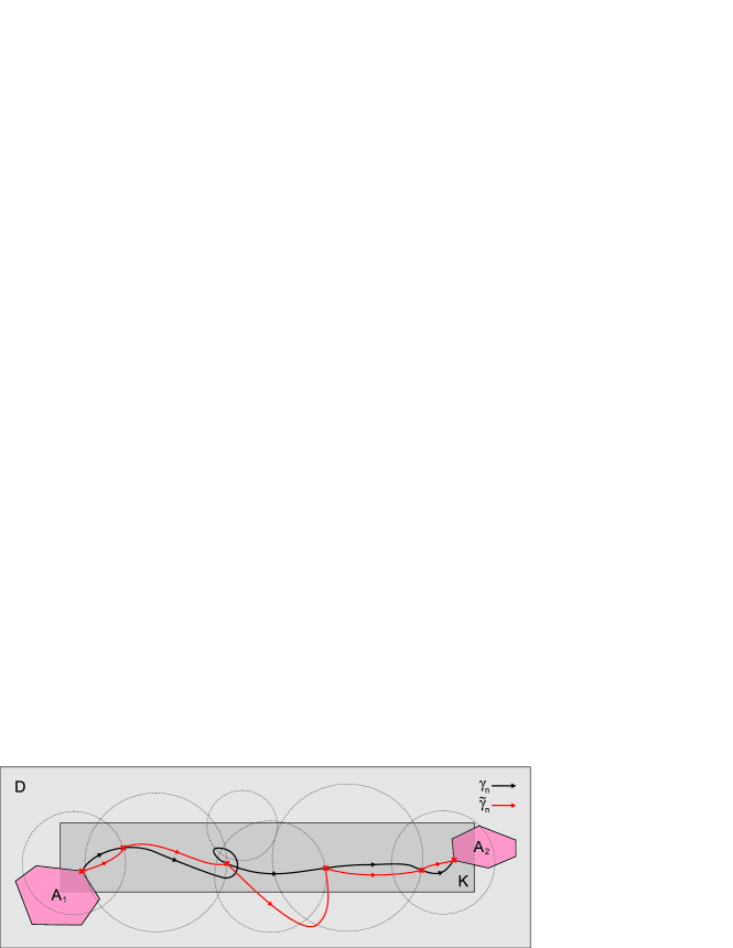
(i) For this part we begin as in the proof of part (ii), by choosing a finite collection of balls $B_{r_{j}}(x_{j})$ covering $K$, now given by Definition 7 (ii) whenever $x_{j}$ only has weak local minimizers. Given the minimizing sequence $(\gamma_{n})_{n\in\mathbb{N}}\subset\Gamma_{A_{1}}^{A_{2}}$, we cut each curve $\gamma_{n}$ into smaller segments as in part (ii). The number of pieces $m$ and the indices $j_{1},\dots,j_{m}$ may depend on $n$, but since there are only finitely many combinations, we may pass on to a subsequence (which we again denote by $(\gamma_{n})_{n\in\mathbb{N}}$), such that $m$ and $j_{1},\dots,j_{m}$ are in fact the same for every curve $\gamma_{n}$.

We then construct a new sequence $(\tilde{\gamma}_{n})_{n\in\mathbb{N}}\subset\tilde{\Gamma}_{A_{1}}^{A_{2}}$ with $S(\tilde{\gamma}_{n})\leq S(\gamma_{n})$ for $\forall n\in\mathbb{N}$ as in the proof of part (ii), only that now if $x_{j_{i}}$ only has weak local minimizers then the curve segment $\gamma^{\star}_{n,i}$ must be obtained from Definition 7 (ii), and so we have $\gamma^{\star}_{n,i}\in\tilde{\Gamma}(x_{j_{i}})$ in this case. We can assume that each segment $\gamma^{\star}_{n,i}$ visits the point $x_{j_{i}}$ at most once (otherwise we can cut out the piece between the first and the last hitting point of $x_{j_{i}}$, which can only decrease the action of the curve).

If $x_{j_{1}}$ has strong local minimizers then we can apply Lemma 2, just as in the proof of Proposition 1, to show that some subsequence of the arclength parameterizations $(\varphi_{n,1})_{n\in\mathbb{N}}\subset\bar{C}(0,1)$ of $(\gamma^{\star}_{n,1})_{n\in\mathbb{N}}$ converges uniformly to the parameterization of some $\gamma^{\star}_{\infty,1}\in\Gamma$. If instead $x_{j_{1}}$ only has weak local minimizers then we apply Lemma 3 to show that a subsequence of some parameteriations $(\varphi_{n,1})_{n\in\mathbb{N}}\subset\tilde{C}(x_{j_{i}})$ of $(\gamma^{\star}_{n,1})_{n\in\mathbb{N}}$ converges pointwise on $[0,1]$ and uniformly on each set $[0,\frac{1}{2}-a]\cup[\frac{1}{2}+a,1]$, $a\in(0,\frac{1}{2})$, to the parameterization of some some $\gamma^{\star}_{\infty,1}\in\tilde{\Gamma}(x_{j_{1}})$. In either case, since $\gamma^{\star}_{n,1}\subset\tilde{D}$ for $\forall n\in\mathbb{N}$ and since $\tilde{D}$ is closed in $D$, we have $\gamma^{\star}_{\infty,1}\subset\tilde{D}$.

We repeat this procedure for $x_{j_{2}},\dots,x_{j_{m}}$, each time passing on to a further subsequence, and in this way obtain curve pieces $\gamma^{\star}_{\infty,1},\dots,\gamma^{\star}_{\infty,m}$ that by construction connect to a curve $\gamma^{\star}\in\tilde{\Gamma}_{A_{1}}^{A_{2}}$. Using both parts of Lemma 5, its action fulfills

$$S(\gamma^{\star}) =\sum_{i=1}^{m}S(\gamma^{\star}_{\infty,i})\leq\sum_{i=1}^{m}\liminf_{n\to\infty}S(\gamma^{\star}_{n,i})\leq\liminf_{n\to\infty}\sum_{i=1}^{m}S(\gamma^{\star}_{n,i})$$

$$=\liminf_{n\to\infty}S(\tilde{\gamma}_{n})\leq\liminf_{n\to\infty}S(\gamma_{n})=\inf_{\gamma\in\Gamma_{A_{1}}^{A_{2}}}S(\gamma)=\inf_{\gamma\in\tilde{\Gamma}_{A_{1}}^{A_{2}}}S(\gamma),$$

where in the last step we used Lemma 12. Since $\gamma^{\star}\in\tilde{\Gamma}_{A_{1}}^{A_{2}}$, equality must hold, and so $\gamma^{\star}$ is a weak minimizer. ∎

Remark 3.

Denoting the minimizer by $\gamma^{\star}$, the proof implies that
in (i), there exists a finite set $W\subset K$ of points that only have weak but not strong local minimizers, depending only on $K$ but not on $A_{1}$ and $A_{2}$, such that every point that $\gamma^{\star}$ passes in infinite length is in $W$;
in (ii), we have $\operatorname*{length}(\gamma^{\star})\leq M$, where $M>0$ is a constant only depending on $K$ but not on $A_{1}$ and $A_{2}$.

Remark 4.

Theorem 1 and Lemma 13 can easily be generalized to cover also the minimization over sets of the form

$$\Gamma_{A_{1},\dots,A_{k}} :=\big{\{}\gamma\subset\tilde{D}\,\big{|}\,\text{\emph{$\gamma$ visits $A_{1},\dots,A_{k}$ in this order}}\big{\}}$$

$$\text{or}\qquad\Gamma_{A_{1},\dots,A_{k}}^{\prime} :=\big{\{}\gamma\subset\tilde{D}\,\big{|}\,\text{\emph{$\gamma$ visits $A_{1},\dots,A_{k}$ in any order}}\big{\}}$$

for any given $k\in\mathbb{N}$ and any given sets $A_{1},\dots,A_{k}\subset\tilde{D}$ that are closed in $D$. In this case, $(\gamma_{n})_{n\in\mathbb{N}}$ must be a minimizing sequence of the corresponding associated minimization problem.

3.3 Finding Points with Local Minimizers

This leaves us with the question how one can show that a given point $x\in\tilde{D}$ has local minimizers. We have developed three criteria, given by Propositions 2, 3 and 4, which were designed to cover the three cases listed in Table 1. In the special case of a Hamiltonian geometric action $S\in\mathcal{H}$ with the choice of a natural drift $b(x)=H_{\theta}(x,0)$, these three cases can be expressed in terms of the Hamiltonian $H$ associated to $S$. The proofs of most statements that are listed in this section will be carried out in Part II.

We will from now on assume that $S\in\mathcal{G}$ and that $b$ is a drift of $S$, and we will denote by $\psi(x,t)$ the flow of $b$ given in Definition 3. Our first result is the following.

	$S\in\mathcal{G}$	$S\in\mathcal{H}$ with natural drift $b$
Prop. 2	$\ell(x,y)>0$ for $\forall y\neq 0$	$H(x,0)<0$
Prop. 3	$\ell(x,y)=0$ for some $y\neq 0$ $b(x)\neq 0$	$H(x,0)=0$ and $H_{\theta}(x,0)\neq 0$
Prop. 4	$\ell(x,y)=0$ for some $y\neq 0$ $b(x)=0$	$H(x,0)=0$ and $H_{\theta}(x,0)=0$

Table 1: The situations for which our criteria Propsitions 2-4 were designed.

Proposition 2.

Let $x\in\tilde{D}$ be such that $\ell(x,y)>0$ for $\forall y\in\mathbb{R}^{n}\setminus\{0\}$. Then $x$ has strong local minimizers.

Proof.

See Part II, Section 2.1. ∎

By Lemma 7 (ii) for actions $S\in\mathcal{H}$ the condition of Proposition 2 is fulfilled if and only if $H(x,0)<0$ for some (and thus every) Hamiltonian $H$ that induces $S$. Unfortunately, this means that Proposition 2 cannot be applied to actions $S\in\mathcal{H}_{0}$, and in particular it cannot be applied to the large deviation geometric actions for SDEs and for Markov jump processes, as given in Example 1. For actions $S\in\mathcal{H}\setminus\mathcal{H}_{0}$ such as the ones given in Examples 2 and 3, however, this criterion is essential (and the easiest one to use); see Example 10 in Section 3.4.3.

To control the potential problems that can arise if $\ell(x,y)=0$ for some $y\neq 0$, we now introduce the concept of admissible manifolds. Loosely speaking, an admissible manifold $M$ is a compact $C^{1}$-manifold of codimension 1 with the property that the flowlines of the drift $b$ are never tangent to $M$ and always cross $M$ in the same direction (“in” or “out”).

Definition 8.

Given a vector field $b\in C^{1}(D,\mathbb{R}^{n})$, a set $M\subset D$ is called an admissible manifold of $b$ if there exists a function $f_{M}\in C(D,\mathbb{R})$ such that
(i) $M=f_{M}^{-1}(\{0\})$, (ii) $M$ is compact, (iii) $f_{M}$ is $C^{1}$ in a neighborhood of $M$, and (iv) $\forall x\in M\colon\,{\langle\nabla f_{M}(x),b(x)\rangle}>0$.

Property (iv) says that the drift vector field $b(x)$ flows from the set $f_{M}^{-1}\big{(}(-\infty,0)\big{)}$ into the set $f_{M}^{-1}\big{(}(0,\infty)\big{)}$ at every point of their common boundary $M=f_{M}^{-1}(\{0\})$, crossing $M$ at a non-vanishing angle. Note that $M$ is a proper $C^{1}$-manifold since by part (iv) we have $\nabla f_{M}\neq 0$ on $M$. Also by part (iv) we have the following:

Remark 5.

If $M$ is an admissible manifold of $b$ then $\forall x\in M\colon\,b(x)\neq 0$.

To get a better idea of how admissible manifolds look in $\mathbb{R}^{2}$, the reader may briefly skip ahead and take a look at Figures 6-8 on pages 6-8. There, the black and the blue lines are the flowlines of the vector field $b(x)$, and the solid red lines are admissible manifolds. Dashed red lines are examples of curves that are not admissible manifolds since they are crossed by the flowlines in either direction (both “in” and “out”).

A simple explicit example can be given for the drift of Example 4, i.e. if $b=-\nabla V$ for some potential $V\in C^{1}(\mathbb{R}^{n},\mathbb{R})$ with $\lim_{x\to\infty}V(x)=\infty$: Here, the level sets $M_{c}:=V^{-1}(\{c\})$, $c\in\mathbb{R}$, are admissible manifolds, provided that $\nabla\nabla V\neq 0$ on $M_{c}$. Indeed, the reader can easily check that all four properties in Definition 8 are fulfilled, with $f_{M_{c}}=-V+c$.

Lemma 14 below gives the simplest general example of an admissible manifold, as found repeatedly in Figures 6-8: the surface of a small deformed ball around a stable or unstable equilibrium point. To prepare for this lemma, we introduce two functions $f_{s}$ and $f_{u}$ that are defined on the basins of attraction/repulsion of $x$, denoted by $B_{s}$ and $B_{u}$, respectively. These functions measure the “distance” of a point $w$ to the equilibrium point $x$ in terms of the length of the flowline starting from $w$ until it reaches $x$ as $t\to\infty$ ($f_{s}$) or as $t\to-\infty$ ($f_{u}$), respectively.

Definition 9.

Let $x\in D$ be such that $b(x)=0$ and that all the eigenvalues of the matrix $\nabla b(x)$ have negative (positive) real part, and let $B_{s}$ ($B_{u}$) be the basin of attraction (repulsion) of $x$. Then we define the function$f_{s}\colon B_{s}\to[0,\infty)$ ($f_{u}\colon B_{u}\to[0,\infty)$) by

$$f_{s}(w) :=\int_{0}^{\infty}|b(\psi(w,t))|\,dt=\int_{0}^{\infty}|\dot{\psi}(w,t)|\,dt,\qquad w\in B_{s},$$ (3.5a)

$$f_{u}(w) :=\int_{-\infty}^{0}\!|b(\psi(w,t))|\,dt=\int_{-\infty}^{0}\!|\dot{\psi}(w,t)|\,dt,\qquad w\in B_{u}.$$ (3.5b)

Lemma 14.

Let $x\in D$ be such that $b(x)=0$ and that all the eigenvalues of the matrix $\nabla b(x)$ have negative (positive) real parts. Then for sufficiently small $a>0$ the level set $M_{s}^{a}:=f_{s}^{-1}(\{a\})$ ($M_{u}^{a}:=f_{u}^{-1}(\{a\})$) is an admissible manifold.

Proof.

See Part II, Section 2.2. ∎

The following Proposition 3, which is our second criterion for showing that a given point $x\in D$ has local minimizers, is our first result that makes use of the concept of admissible manifolds. In practice this criterion covers most cases which cannot be treated with Proposition 2.

Proposition 3.

Let $M$ be an admissible manifold and $x\in\psi(M,\mathbb{R})\cap\tilde{D}$. Then $x$ has strong local minimizers.

Proof.

See Part II, Section 2.5. ∎

Proposition 3 says that every admissible manifold $M$ that we find will give us a whole region $\psi(M,\mathbb{R})\cap\tilde{D}$ of points with strong local minimizers, consisting of all the flowlines emanating from $M$. An immediate consequence is the following:

Corollary 1.

Let $x\in\tilde{D}$ be such that $b(x)=0$ and that all the eigenvalues of the matrix $\nabla b(x)$ have negative (positive) real parts, and denote by $B_{s}$ ($B_{u}$) the basin of attraction (repulsion) of $x$. Then every point in $(B_{s}\setminus\{x\})\cap\tilde{D}$ ($(B_{u}\setminus\{x\})\cap\tilde{D}$) has strong local minimizers.

Proof.

This follows from Lemma 14 and Proposition 3 since for small $a>0$ we have $\psi(M_{s}^{a},\mathbb{R})=B_{s}\setminus\{x\}$ and $\psi(M_{u}^{a},\mathbb{R})=B_{u}\setminus\{x\}$. (The reader who wants to prove these intuitive equations rigorously will find the necessary tools in Lemma 20.) ∎

By Remark 5, admissible manifolds cannot contain any points $x$ with $b(x)=0$, and thus the flowlines emanating from $M$ cannot contain any such points either. As a consequence, to show that a given point $x\in\tilde{D}$ has local minimizers, Proposition 3 can only be useful if $b(x)\neq 0$. For points with $b(x)=0$ (and in particular for the missing point $x$ in Corollary 1) we have the following criterion.

Proposition 4.

Let $x\in\tilde{D}$ be such that $b(x)=0$, and that all the eigenvalues of the matrix $\nabla b(x)$ have nonzero real part. Let us denote by $M_{s}$ and $M_{u}$ the global stable and unstable manifolds of $x$, respectively, i.e.

$$M_{s} :=\big{\{}w\in D\,\big{|}\,\lim_{t\to\infty}\psi(w,t)=x\big{\}},$$ (3.6a)

$$M_{u} :=\big{\{}w\in D\,\big{|}\,\lim_{t\to-\infty}\psi(w,t)=x\big{\}}.$$ (3.6b)

(i) If $x$ is an attractor or repellor of $b$ then $x$ has weak local minimizers. If in addition

$$\exists\varepsilon,c_{3}>0 \forall w\in\bar{B}_{\varepsilon}(x)\cap\tilde{D} \exists\gamma\in\Gamma_{x}^{w}\colon \operatorname*{length}(\gamma) \leq c_{3}|w-x|,$$ (3.7)

$$\exists\rho,c_{4},\delta>0 \forall w\in\bar{B}_{\rho}(x) \forall y\in\mathbb{R}^{n}\hskip 0.5pt\colon \ell(w,y) \leq c_{4}|w-x|^{\delta}|y|,$$ (3.8)

then $x$ has strong local minimizers.
(ii) If $x$ is a saddle point, and if there exist admissible manifolds $M_{1},\dots,M_{m}$ such that

$$(M_{s}\cup M_{u})\setminus\{x\}\subset\bigcup_{i=1}^{m}\psi(M_{i},\mathbb{R}),$$ (3.9)

then $x$ has weak local minimizers. If in addition the state space is two-dimensional, i.e. $D\subset\mathbb{R}^{2}$, and if (3.7)-(3.8) are fulfilled then $x$ has strong local minimizers.

Proof.

See Part II, Section 2.6. ∎

The condition (3.7) on the shape of the set $\tilde{D}$ near $x$ is a stronger version of Assumption ($\tilde{D}$), and it is violated only in degenerate cases that are rarely of interest in practice. Lemma 15 (i) will give some useful criteria. The condition (3.8) can also easily be checked, even in the case of a Hamiltonian geometric action when no explicit formula for $\ell(x,y)$ may be available; see Lemma 15 (ii).

Lemma 15.

(i) If $x\in\tilde{D}^{\circ}$ (which is true in particular if $\tilde{D}=D$), or if $\tilde{D}=\bigcup_{i=1}^{m}\tilde{D}_{i}$ for some sets $\tilde{D}_{1},\dots,\tilde{D}_{m}\subset D$ that are convex and closed in $D$, then the condition (3.7) is fulfilled.
(ii) Suppose that $S\in\mathcal{H}$ is induced by a Hamiltonian $H$ such that $H(\,\cdot\,,0)$ and $H_{\theta}(\,\cdot\,,0)$ are locally Hölder continuous at $x$. Then the condition (3.8) is fulfilled if and only if $x$ is a critical point.

Proof.

(i) As in the proof of Lemma 11. (ii) See Appendix A.5. ∎

The condition (3.9) says that every point in the stable and unstable manifold of $x$ (except for $x$ itself) has to lie on a flowline emanating from one of a finite collection of admissible manifolds, or equivalently, that every flowline in the stable and the unstable manifold must intersect one of these finitely many admissible manifolds. See the next section for examples.

Finally, it should be pointed out that it is Proposition 4 (ii) that is responsible for the excessive length of our proofs (and in particular for all of Part III). In particular, a lot of effort in part (ii) went into proving the existence of strong local minimizers at least in the two-dimensional case, which allows us to conclude that the problem $P(A_{1},A_{2})$ of minimizing $S(\gamma)$ over all $\gamma\in\Gamma_{A_{1}}^{A_{2}}$ has a solution $\gamma^{\star}$ that actually lies in $\Gamma_{A_{1}}^{A_{2}}$ and not only in the larger class $\tilde{\Gamma}_{A_{1}}^{A_{2}}$. For remarks on the possible extension of our results to higher dimensions, see the Conclusions in Chapter 5.

3.4 Examples in $\mathbb{R}^{2}$

Let us see in some two-dimensional examples, $D=\mathbb{R}^{2}$, how these criteria are used in practice. In Figures 6-8, the black and the blue lines are the flowlines of $b$, the roots of $b$ are denoted by the symbols $\ominus$ (attractor), $\oplus$ (repellor) and $\circledS$ (saddle point). Basins of attraction are shown in various shades of gray, basins of repulsion are drawn in gray lines at various angles. The stable and unstable manifolds of the saddle points are drawn in blue. Finally, a representative selection of admissible manifolds is drawn as red solid curves. In Fig. 8, dashed red curves illustrate why it is impossible to draw admissible manifolds through certain points.

Throughout the discussion of these examples (i.e. in the remainder of Section 3.4) we will assume that for every root $x$ of $b$ (i.e. for every attractor, repellor, or saddle point) all the eigenvalues of the matrix $\nabla b(x)$ have non-zero real parts. Also, for simplicity we will discuss the case $\tilde{D}=D$, so that the condition (3.7) is trivially fulfilled by Lemma 15 (i). But our arguments will not change if $\tilde{D}\subsetneq D$, except that then proving that the roots of $b$ have strong (as opposed to weak) local minimizers requires checking the additional condition (3.7), e.g. by using Lemma 15 (i).

3.4.1 Two basins of attraction

In our first two examples we consider systems in which the drift vector field $b$ has two stable equilibrium points whose basins of attraction partition the state space into two regions.

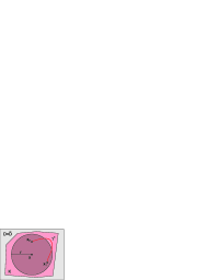
Example 5.

Fig. 6 (a) shows the flowlines of a vector field $b$ with two attractors, and with one saddle point on the separatrix. The points in the two basins of attraction (shaded in light gray and dark gray) all have local minimizers by Corollary 1 and Proposition 4 (i). The three red lines are admissible manifolds (the two small ones can be obtained from Lemma 14), and we observe that every flowline on the stable and the unstable manifold of the saddle point (blue) intersects one of them. Proposition 3 thus implies that every point on these flowlines has local minimizers, and Proposition 4 (ii) implies that the saddle point itself has local minimizers as well. We conclude that in this system every point in $\tilde{D}$ has local minimizers.

In fact, all points (with the possible exception of the roots of $b$) have strong local minimizers. To guarantee that the three roots have strong local minimizers as well, one only needs to check the condition (3.8) at these points. In the case of an action $S\in\mathcal{H}$ induced by some Hamiltonian $H$ such that $H(\,\cdot\,,0)$ and $H_{\theta}(\,\cdot\,,0)$ are locally Hölder continuous, by Lemma 15 this is equivalent to (2.10). In particular, if $S\in\mathcal{H}_{0}$ and $b$ is a natural drift then there is nothing to check. These remarks about the distinction between strong and weak local minimizers also apply to the Examples 6-9. ∎

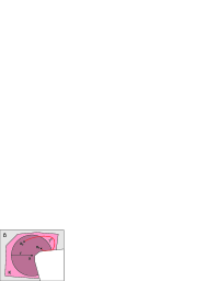
Example 6.

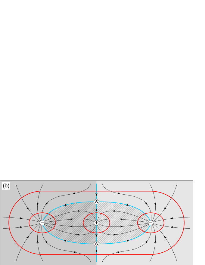
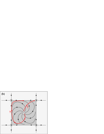
Fig. 6 (b) shows another system with two attractors, only now there are two saddle points and one repellor on the separatrix. The points in the two basins of attraction are again shaded in light gray and dark gray, the basin of repulsion is drawn in gray diagonal lines. By Corollary 1 and Proposition 4 (i) every point in these three regions has local minimizers, which leaves us only with the two saddle points, and with the outer halves of their respective stable manifolds. Again we observe that every flowline of the stable and unstable manifolds of the two saddle points (blue) intersects one of the four admissible manifolds drawn in the figure. As in the previous example, Proposition 3 thus implies that every point on these flowlines has local minimizers, and Proposition 4 (ii) implies that the two saddle points have local minimizers as well. We conclude that also in this system every point in $\tilde{D}$ has local minimizers. ∎

Figure 6: Two systems with two attractors, and one system with three attractors.

Figure 7: Two more systems with three attractors.

3.4.2 Three basins of attraction

We now discuss three examples of systems with three attractors. In each case, we will again find that every point in the state space has local minimizers.

Example 7.

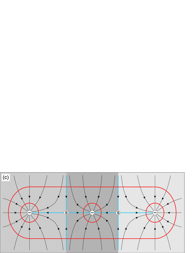
Fig. 6 (c) shows a system with three attractors, with all three basins of attraction aligned in a row. As usual, Corollary 1 and Proposition 4 (i) cover the three basins of attraction, Proposition 3 covers the stable manifolds of the saddle points since they intersect the outer admissible manifold, and Proposition 4 (ii) covers the saddle points themselves since every flowline of their stable and unstable manifolds intersects an admissible manifold. We conclude again that every point in $\tilde{D}$ has local minimizers. ∎

Example 8.

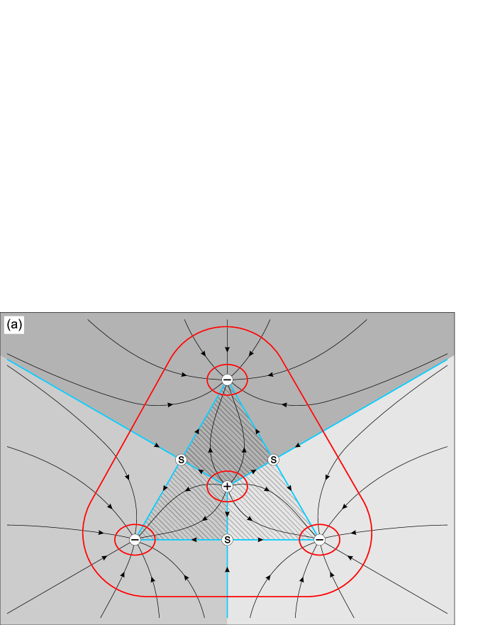
Fig. 7 (a) shows a system with three attractors that form a triangle with a repellor at its center. There are a total of three saddle points, one on each of the three branches of the separatrix. All the points in the three basins of attraction and in the basin of repulsion have local minimizers by Corollary 1 and Proposition 4 (i). Again we are left only with the three saddle points, and with the outer halves of their stable manifolds. Both can be treated with Propositions 3 and 4 (ii) as in the previous examples, and we find again that every point in $\tilde{D}$ has local minimizers. ∎

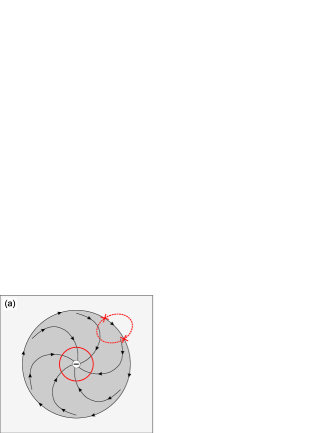
Example 9.

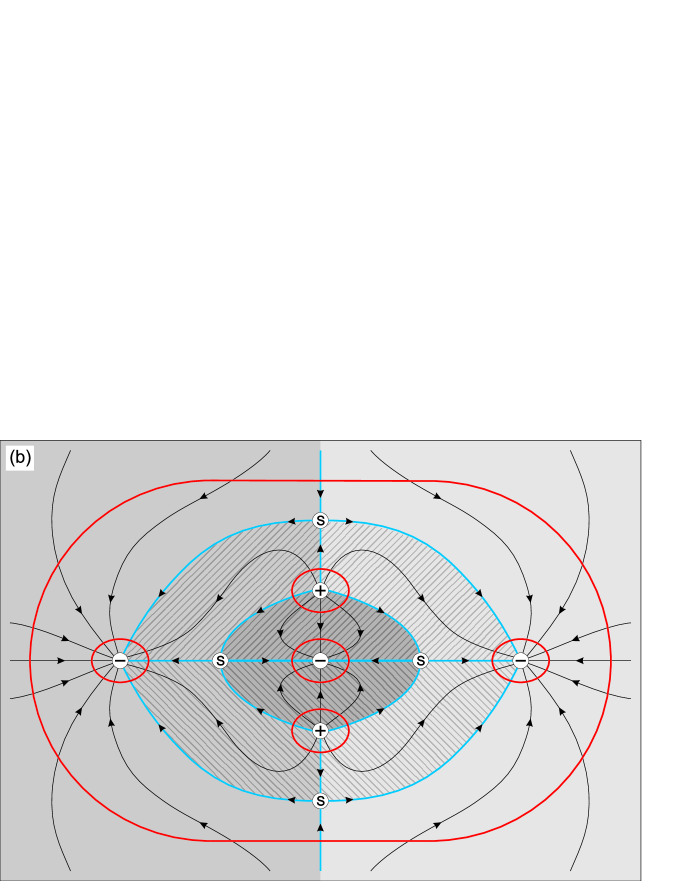
Fig. 7 (b) shows yet another system with three attractors. This time, one basin of attraction is enclosed by the two others, and we count a total of two repellors and four saddle points. After applying Corollary 1 and Proposition 4 (i) to the three basins of attraction and the two basins of repulsion, we are only left with the four saddle points, and with the outer halves of the stable manifolds of the two outer saddle points. We can proceed as before, and apply Propositions 3 and 4 (ii) to show that also these remaining points have local minimizers. ∎

3.4.3 An example with trivial natural drift

Example 10.

For the geometric action given by (2.21), i.e. the curve length with respect to a Riemannian metric, and for the quantum tunnelling geometric action given by (2.22) in Section 2.3 we only found the natural drift $b(x)\equiv 0$, and so we must argue differently. In the first case we have $\ell(x,y)>0$ for $\forall y\neq 0$ by our assumption that $A(x)$ is positive definite, and so every point $x\in\tilde{D}$ has strong local minimizers by Proposition 2.

For the quantum tunnelling geometric action this argument applies only to all points $x\in\tilde{D}\setminus\{x_{1},x_{2}\}$ (where $U(x)>0$), and we will have to deal with the points $x=x_{1},x_{2}$ separately. Let us now assume that $\exists c,\varepsilon>0$ $\forall x\in B_{\varepsilon}(x_{i})\colon$ $|U(x)|\geq c|x-x_{i}|^{2}$, $i=1,2$.

Then the vector fields $b_{i}(x):=\zeta_{i}(x)(x-x_{i})$, for some cutoff functions $\zeta_{i}\in C^{1}(D,[0,1])$ with $\operatorname*{supp}\zeta_{i}\subset B_{\varepsilon}(x_{i})$ and $\zeta_{i}(x_{i})=1$, are drift vector fields of $S$ since

$$\ell(x,y)=\sqrt{2U(x)}\,|y| \geq\sqrt{2c}\,\zeta_{i}(x)|x-x_{i}||y|=\sqrt{2c}\,|b_{i}(x)||y|$$

$$\geq\sqrt{c/2}\,\big{(}|b_{i}(x)||y|-{\langle b_{i}(x),y\rangle}\big{)}.$$

Since $x_{i}$ is a repellor of $b_{i}(x)$ with $\nabla b_{i}(x_{i})=I$, we can apply Proposition 4 (i) to conclude that $x_{1}$ and $x_{2}$ have weak local minimizers. If in addition $U$ is Hölder continuous at $x_{1}$ and $x_{2}$ then the condition (3.8) is fulfilled, and $x_{1}$ and $x_{2}$ have in fact strong local minimizers. (Observe that the alternative criterion for (3.8) given by Lemma 15 leads to the same condition.) ∎

3.4.4 Examples to which our criteria do not apply

We will now present three examples in which for some points the conditions of our criteria are not fulfilled. As a consequence, unless we can otherwise show that there exists a minimizing sequence that stays in a compact set $K\subset\tilde{D}$ away from these points, the question of whether a minimizer exists will be left undecided at present: Without further thought it may still be possible that (i) the points in question in fact do have local minimizers, and our criteria from the previous section are only not strong enough to show it, or (ii) the points do not have local minimizers, but Theorem 1 which requires this property for all points in the compact set $K\subset\tilde{D}$ is asking for more than necessary. In both cases a minimizer may still exist.

Fortunately, for the first of the following examples we will discover later in Chapter 4 that (at least for actions $S$ in the subclass $\mathcal{H}_{0}^{+}\subset\mathcal{H}_{0}$ defined at the beginning of Chapter 4) both Theorem 1 and our criteria in fact fail for a reason, and that the above possibilities (i) and (ii) are not the case: Proposition 5 will show that for these actions the points in question do not have local minimizers and that a minimizer does not exist. For the second example we will have a partial result of that kind. These insights are an important contribution to our theory because they indicate why the conditions of our criteria are necessary, and they suggest that they are not unnecessarily strong.

These first two examples have in common that there is a loop consisting of one or more flowlines that can be traversed at no cost. Such loops are bound to lead to problems since they allow for infinitely long curves with zero action, thus making it hard to control the curve lengths of a minimizing sequence.

Figure 8: Three systems to which our criteria cannot be applied.

Figure 9: The (generalized) minimum action curves for two of these cases.

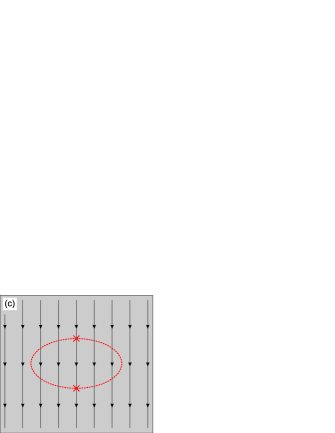
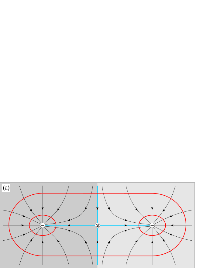
Limit cycles.

Fig. 8 (a) shows a system consisting of a limit cycle which encloses the basin of attraction of a stable equilibrium point. We are interested in a curve of minimal action that leads from the attractor to the limit cycle, and so the vector field outside of the limit cycle is irrelevant to us.

All the points in the basin of attraction can again be treated by Corollary 1 and Proposition 4 (i), but (independently of the drift vector field outside of the limit cycle) our criteria will fail to show that the points on the limit cycle itself have local minimizers: Proposition 3 would require us to find an admissible manifold that crosses the limit cycle, but this is impossible.

Indeed, any closed loop $M$ that may be a candidate for an admissible manifold crossing the limit cycle (such as the red dashed line in Fig. 8 (a)) would have to intersect the limit cycle at least twice (it is not allowed to be tangent to the limit cycle by Definition 8 (iv)), or put differently, the limit cycle would have to intersect $M$ at least twice. But this would mean that the flowline on the limit cycle enters the interior of $M$ at one place and exits it at another (at the two red crosses), contradicting of Definition 8 (iv). This observation is proven rigorously in Corollary 3 of Part II.

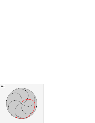
In Section 4.3 we will prove that all this happens for a reason: Proposition 5 says that for actions $S\in\mathcal{H}_{0}^{+}$, points on limit cycles never have (weak or strong) local minimizers, and that no minimizer from the attractor (in fact from any point in the basin of attraction) to the limit cycle exists. Instead, the cheapest way to approach the limit cycle is to circle around infinitely in the direction of the flow, see Fig. 9 (a); this however is not a curve in $\tilde{\Gamma}$ and is thus not considered a valid minimizer in our, present framework.

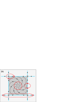
Closed chains of flowlines.

The next example in Fig. 8 (b) is similar in character: Again we have a closed curve that can be traversed at no cost, only that this time it consists of four flowlines that lead from saddle point to saddle point, and we are looking for a curve of minimal action that leads from the attractor to this loop. As before, our criteria fail to show that any of the points on the loop has local minimizers: Both Proposition 3 and 4 (ii) would require us to find an admissible manifold crossing the loop, but for the same reasons as in the previous example this can easily be seen to be impossible.

This time however, the issue can at present not be resolved entirely. Corollary 2 in Section 4.3 only allows us to conclude for actions $S\in\mathcal{H}_{0}^{+}$ that if a minimizer exists then it will reach the loop at one of the saddle points. Further work would be necessary to prove that such a solution indeed exists, and to decide if it is more advantageous to rather approach the loop by circling around infinitely in the direction of the flow, see Fig. 9 (b).

At least Lemma 19 explains why our criteria are insufficient for showing that those points on the loop with non-zero drift have local minimizers: The proofs of these criteria work by proving the stronger requirements of Remark 2 (ii), and for actions $S\in\mathcal{H}_{0}^{+}$ those are not fulfilled.

Non-contracting state space.

The examples of Sections 3.4.1 and 3.4.2 had in common that the state space was contracting in the sense that there exists a bounded region which every flowline eventually leads into as $t\to\infty$. This last example, a constant vector field $b(x):\equiv b_{0}\neq 0$ illustrated in Fig. 8 (c), discusses what can happen if that is not the case.

For reasons similar to the ones in the previous two examples we fail to find even a single admissible manifold, and so we cannot apply Proposition 3. However, at least in the simple case of the geometric action for an SDE with non-vanishing constant drift and with additive noise it is not difficult to adjust the technique of this paper and to show that every point has strong local minimizers: At the beginning of Section 2.4 we will show how in this case one can effectively use the non-compact admissible manifold $M=\{b_{0}\}^{\perp}$.

It may be possible to extend the results of this paper to cover also cases like this one in more generality: One could drop the assumption that admissible manifolds need to be compact and instead list all the entities that need to be bounded on them, leading to a more technical definition of admissible manifolds. This however would go beyond the scope of our work at this point.

4 Properties of Minimum Action Curves

Let us begin by defining the subclass $\mathcal{H}_{0}^{+}\subset\mathcal{H}_{0}$ of geometric actions to which most results in this chapter apply. Observe that this class includes the large deviation geometric actions in Example 1.

Definition 10.

We define $\mathcal{H}_{0}^{+}\subset\mathcal{H}_{0}$ as the class of all Hamiltonian geometric actions that are induced by a Hamiltonian that fulfills the Assumptions (H1’), (H3), and the following stronger smoothness assumption:
​(H2’) The derivatives $H_{x}$, $H_{\theta}$, $H_{x\theta}=(H_{\theta x})^{T}$, $H_{\theta\theta}$ and $H_{x\theta\theta}$ exist and are continuous in $(x,\theta)$.

Note that for $S\in\mathcal{H}_{0}^{+}$ we cannot guarantee that every Hamiltonian that induces $S$ will fulfill (H2’). Also recall that by Lemma 7 (i), for these actions a point $x\in\tilde{D}$ is critical if and only if $b(x)=0$.
The goal of this chapter is to study some properties of geometric actions and their minimizers. Our main results (for simplicity stated for the case $\tilde{D}=D$) are summarized below. While the first result applies to general geometric actions, the last three only hold for actions $S\in\mathcal{H}_{0}^{+}$ with a corresponding natural drift $b$.

• The only points that a curve $\gamma\in\tilde{\Gamma}$ with $S(\gamma)<\infty$ can pass in infinite length are those at which every drift of $S$ vanishes.

• If $L$ is a limit cycle of $b$ and if $A_{1}\subset D\setminus L$ then the minimization problem $P(A_{1},L)$ does not have a solution. We give a quantitative explanation why curves rather like to approach $L$ by circling around infinitely in the direction of the flow.

• Points on limit cycles of $b$ do not have local minimizers.

• Minimum action curves leading from one attractor of $b$ to another reach and leave the separatrix between the two basins of attraction at critical points (see Fig. 10).

4.1 Points that are Passed in Infinite Length

To prepare for Corollary 2, we need to understand which points can be passed in infinite length without accumulating infinite action. Here we find that such points must be roots of any drift $b$. A refined statement relating the length of a curve to its action is given by Lemma 26 in Part II.

Lemma 16.

Let $S\in\mathcal{G}$, let $\gamma\in\tilde{\Gamma}$ with $S(\gamma)<\infty$, and let $x$ be a point on $\gamma$ that is passed in infinite length. Then for every drift $b$ of $S$ we have $b(x)=0$.

Proof.

Suppose that $b_{0}:=b(x)\neq 0$. Let $\varepsilon>0$ be so small that $\bar{B}_{\varepsilon}(x)\subset D$,

$$c:=\min_{w\in\bar{B}_{\varepsilon}(x)}|b(w)|>0\qquad\text{and}\qquad\min_{w\in\bar{B}_{\varepsilon}(x)}{\big{\langle}\hat{b}_{0},\widehat{b(w)}\big{\rangle}}\geq\tfrac{1}{2},$$

where we use the notation $\hat{v}:=\frac{v}{|v|}$ for $\forall v\in\mathbb{R}^{n}\setminus\{0\}$, and let $c_{2}:=c_{2}(\bar{B}_{\varepsilon}(x))$. By passing on to a small segment of $\gamma$ around $x$, it is enough to consider the case $\gamma\in\tilde{\Gamma}(x)$, and we may assume that $\gamma\subset\bar{B}_{\varepsilon}(x)$. We will obtain a contradiction by showing that $S(\gamma)=\infty$.

To do so, let $\varphi\in\tilde{C}(x)$ be a parameterization of $\gamma$, and define for$\forall a\in(0,\frac{1}{2})$ the sets $I_{a}:=[0,\frac{1}{2}-a]\cup[\frac{1}{2}+a,1]$ and $I_{a}^{-}:=\{\alpha\in I_{a}\,|\,\varphi^{\prime}(\alpha)\neq 0\}$ and the number $L_{a}:=\int_{I_{a}}|\varphi^{\prime}|\,d\alpha$. Then

$$\int_{I_{a}^{-}}|\varphi^{\prime}|\big{|}\widehat{b(\varphi)}-\widehat{\varphi^{\prime}}\big{|}\,d\alpha \geq\int_{I_{a}^{-}}|\varphi^{\prime}|{\big{\langle}\hat{b}_{0},\widehat{b(\varphi)}-\widehat{\varphi^{\prime}}\big{\rangle}}\,d\alpha\geq\int_{I_{a}}\big{(}\tfrac{1}{2}|\varphi^{\prime}|-{\big{\langle}\hat{b}_{0},\varphi^{\prime}\big{\rangle}}\big{)}\,d\alpha$$

$$=\tfrac{1}{2}L_{a}-{\big{\langle}\hat{b}_{0},\big{[}\varphi(\tfrac{1}{2}-a)-\varphi(0)\big{]}+\big{[}\varphi(1)-\varphi(\tfrac{1}{2}+a)\big{]}\big{\rangle}}$$

$$\geq\tfrac{1}{2}L_{a}-4\varepsilon,$$

which is positive for small $a$ since $\lim_{a\searrow 0}L_{a}=\operatorname*{length}(\gamma)=\infty$. By (2.6) and the Cauchy-Schwarz inequality this implies that

$$S(\gamma) \geq\int_{I_{a}^{-}}\ell(\varphi,\varphi^{\prime})\,d\alpha\geq c_{2}\int_{I_{a}^{-}}\big{(}|b(\varphi)||\varphi^{\prime}|-{\big{\langle}b(\varphi),\varphi^{\prime}\big{\rangle}}\big{)}\,d\alpha$$

$$=\frac{c_{2}}{2}\int_{I_{a}^{-}}|b(\varphi)||\varphi^{\prime}|\big{|}\widehat{b(\varphi)}-\widehat{\varphi^{\prime}}\big{|}^{2}\,d\alpha\geq\frac{c_{2}c}{2}\int_{I_{a}^{-}}|\varphi^{\prime}|\big{|}\widehat{b(\varphi)}-\widehat{\varphi^{\prime}}\big{|}^{2}\,d\alpha$$

$$\geq\frac{c_{2}c}{2}\cdot\frac{\big{(}\int_{I_{a}^{-}}|\varphi^{\prime}|\big{|}\widehat{b(\varphi)}-\widehat{\varphi^{\prime}}\big{|}\,d\alpha\big{)}^{2}}{\int_{I_{a}^{-}}|\varphi^{\prime}|\,d\alpha}\geq\frac{c_{2}c\big{(}\tfrac{1}{2}L_{a}-4\varepsilon\big{)}^{2}}{2L_{a}},$$

and letting $a\searrow 0$ shows that $S(\gamma)=\infty$. ∎

4.2 The Advantage of Going With the Flow

The next lemma says that the drift $b$ is the only candidate for a direction into which one can move at no cost, and that for actions $S\in\mathcal{H}_{0}$ one can indeed follow the the natural drift flowlines at no cost. Note that the latter is obvious for the geometric action given by (1.7).

Lemma 17.

(i) Let $S\in\mathcal{G}$, let $b$ be a drift of $S$, and let $x\in D$ and $y\in\mathbb{R}^{n}\setminus\{0\}$. If $\ell(x,y)=0$ then either $b(x)=0$ or $y=cb(x)$ for some $c>0$.
(ii) Let $S\in\mathcal{H}_{0}$, let $b$ be a natural drift, and let $x\in D$ and $y\in\mathbb{R}^{n}$. If $b(x)=0$ or $y=cb(x)$ for some $c\geq 0$ then $\ell(x,y)=0$.
(iii) If $S\in\mathcal{H}_{0}$ and $\gamma\in\tilde{\Gamma}$ is a flowline of a natural drift then $S(\gamma)=0$.

Proof.

(i) If $\ell(x,y)=0$ then (2.6) implies that either $b(x)=0$ or $y=cb(x)$ for some $c\geq 0$. Since $y\neq 0$, we must have $c>0$.
(ii) If $0=b(x)=H_{\theta}(x,0)$ then $x$ is a critical point by Lemma 7 (i), so that $\ell(x,y)=0$ for $\forall y\in\mathbb{R}^{n}$. If $b(x)\neq 0$ and $y=cb(x)=cH_{\theta}(x,0)$ for some $c>0$ then $(\vartheta,\lambda)=(0,\frac{1}{c})$ solves (2.11), so that $\vartheta(x,y)=0$ and thus $\ell(x,y)={\langle\vartheta(x,y),y\rangle}=0$ by (2.12). If $c=0$ then $y=0$, and so we have $\ell(x,y)=0$ again.
(iii) Given any parameterization $\varphi\in\tilde{C}(0,1)$ of $\gamma$, we have $\varphi^{\prime}=cb(\varphi)$ a.e. on $[0,1]$ for some function $c(\alpha)\geq 0$, and so part (ii) implies that $\ell(\varphi,\varphi^{\prime})=0$ a.e. on $[0,1]$, i.e. $S(\gamma)=0$. ∎

Now suppose that $S\in\mathcal{H}_{0}$. The next lemma says that if the end of a given curve does not follow the natural drift flowlines (so that its action is positive) then we may reduce its action by bending it slightly into the direction of the drift. This is less obvious than it seems at first since the sheared curves given by (4.2) may also be longer, and so a precise calculation is necessary to show that the benefits from the change in direction outweigh the potential increase in length.

Lemma 18.

Let $S\in\mathcal{H}_{0}^{+}$, and let $b$ be a natural drift of $S$ obtained from a Hamiltonian that fulfills the Assumption (H2’). Let $\gamma\in\Gamma$, let $x$ be its end point, and let $\varphi\in\bar{C}({0,1})$ be its arclength parameterization. Suppose that $b(x)\neq 0$, and that

$$\exists\tau>0\,\ \text{$\exists\!$ arbitrarily large $\alpha\in[0,1)\colon$}\ \,\varphi(\alpha)\notin\psi\big{(}x,(-\tau,0]\big{)}.$$ (4.1)

Then for sufficiently large $\alpha_{0}\in[0,1)$ the family of curves $\gamma_{\varepsilon}\in\Gamma$ given by

$$\varphi_{\varepsilon}(\alpha):=\begin{cases}\varphi(\alpha)&\text{if }\alpha\in[0,\alpha_{0}],\\ \varphi(\alpha)+\varepsilon(\alpha-\alpha_{0})b(\varphi(\alpha))&\text{if }\alpha\in[\alpha_{0},1],\end{cases}$$ (4.2)

defined for small $\varepsilon\geq 0$, fulfills $\partial_{\varepsilon}S(\gamma_{\varepsilon})|_{\varepsilon=0}<0$.

Proof.

See Appendix A.6. ∎

4.3 Some Results on the Non-Existence of Minimizers

Lemma 18 has many useful consequences. The first one is that under certain conditions on $A_{2}$, any solution of $P(A_{1},A_{2})$ must first reach $A_{2}$ at a critical point, since otherwise we could use Lemma 18 to construct a curve with a lower action. In particular, (under these conditions) this means that if $A_{2}$ does not contain any critical points then no minimizer can exist.

Corollary 2.

Let $S\in\mathcal{H}_{0}^{+}$. Let $A_{2}\subset\tilde{D}$ be closed in $D$, let $A_{1}\subset\tilde{D}\setminus A_{2}$, and suppose that the minimization problem $P(A_{1},A_{2})$ has a weak solution $\gamma^{\star}\in\tilde{\Gamma}_{A_{1}}^{A_{2}}$. Denoting by $\hat{x}$ its first hitting point of $A_{2}$, let us also assume that $\hat{x}\in\tilde{D}^{\circ}$ and that the flow $\psi$ of some natural drift $b$ of $S$ fulfills

$$\psi\big{(}\hat{x},(-\tau,\tau)\big{)}\subset A_{2}\text{\qquad for some $\tau>0$.}$$ (4.3)

(In particular, these conditions on $\hat{x}$ are fulfilled if $A_{2}\subset\tilde{D}^{\circ}$ and if $A_{2}$ is flow-invariant under $b$.) Then $\hat{x}$ is a critical point.

Proof.

We may assume that $\hat{x}$ is the end point of $\gamma^{\star}$ (otherwise we may instead consider the minimizer obtained by cutting off the segment after $\hat{x}$). Also, because of Remark 1, (4.3) is in fact fulfilled for the flow of any natural drift of $S$, and thus we may assume that $b$ is constructed from a Hamiltonian that fulfills Assumption (H2’).

Suppose that $b(\hat{x})\neq 0$. Then since $S(\gamma^{\star})<\infty$ by the remark following Assumption ($\tilde{D}$), Lemma 16 says that $\gamma^{\star}$ cannot pass $\hat{x}$ in infinite length, and thus we can write $\gamma^{\star}=\gamma^{1}+\gamma^{2}$, where $\gamma^{2}$ is a rectifiable curve ending in $\hat{x}$ such that $\gamma^{2}\subset\tilde{D}^{\circ}$ and $\operatorname*{length}(\gamma^{2})>0$. Now consider the family of curves $\gamma_{\varepsilon}$ constructed from $\gamma=\gamma^{2}$ as in Lemma 18. The condition (4.1) is fulfilled since $\gamma^{2}$ does not visit $\psi(\hat{x},(-\tau,0])\subset A_{2}$ prior to $\hat{x}$, and so we have $\partial_{\varepsilon}S(\gamma_{\varepsilon})|_{\varepsilon=0}<0$, which implies that $S(\gamma_{\varepsilon})\leq S(\gamma^{2})-c\varepsilon$ for some $c>0$ and all sufficiently small $\varepsilon\geq 0$. Now defining $x_{\varepsilon}:=\psi(\hat{x},\varepsilon(1-\alpha_{0}))$, which by (4.3) is in $A_{2}$ for $\varepsilon\in[0,\tau)$, we have

$$x_{\varepsilon} =\psi(\hat{x},0)+\varepsilon(1-\alpha_{0})\dot{\psi}(\hat{x},0)+o(\varepsilon)$$

$$=\hat{x}+\varepsilon(1-\alpha_{0})b(\hat{x})+o(\varepsilon)$$

$$=\varphi_{\varepsilon}(1)+o(\varepsilon),$$

i.e. the straight line $\bar{\gamma}_{\varepsilon}$ from $\varphi_{\varepsilon}(1)$ (that is the end point of $\gamma_{\varepsilon}$) to $x_{\varepsilon}\in A_{2}$ has a length and thus by Lemma 4 (ii) also an action of order $o(\varepsilon)$. Finally, for sufficiently small $\varepsilon>0$ we have $\gamma_{\varepsilon},\bar{\gamma}_{\varepsilon}\subset\tilde{D}^{\circ}$ and thus $\tilde{\gamma}^{\star}:=\gamma^{1}+\gamma_{\varepsilon}+\bar{\gamma}_{\varepsilon}\in\tilde{\Gamma}_{A_{1}}^{A_{2}}$, and the above estimates show that

$$S(\tilde{\gamma}^{\star}) =S(\gamma^{1})+S(\gamma_{\varepsilon})+S(\bar{\gamma}_{\varepsilon})\leq S(\gamma^{1})+S(\gamma^{2})-c\varepsilon+o(\varepsilon)$$

$$=S(\gamma^{\star})-c\varepsilon+o(\varepsilon)<S(\gamma^{\star})$$

for small $\varepsilon>0$, contradicting the minimizing property of $\gamma^{\star}$. ∎

Two examples of flow-invariant sets $A_{2}$ to which we can apply Corollary 2 are limit cycles and closed chains of flowlines, as shown in Fig. 8 (a) and (b), which leads us to the results that were discussed in Section 3.4.4.

Proposition 5.

Let $S\in\mathcal{H}_{0}^{+}$, let $b$ be a natural drift, and let $L\subset\tilde{D}^{\circ}$ be a limit cycle of $b$, i.e.

$$\exists x\in L\,\ \exists T>0\colon\quad b(x)\neq 0,\ \ L=\psi(x,[0,T))\text{\ \ and\ \ }\psi(x,T)=x.$$

(i) If $A_{1}\subset\tilde{D}\setminus L$ and $A_{2}\subset L$ then the minimization problem $P(A_{1},A_{2})$ does not have any solutions.
(ii) Points $x\in L$ do not have local minimizers.

Proof.

(i) First suppose that $A_{2}=L$. If $P(A_{1},L)$ had a solution $\gamma^{\star}$ then according to Corollary 2 its first hitting point of $L$ would be a critical point. But there are no critical points on $L$, so $P(A_{1},L)$ cannot have a solution.

Now let $A_{2}\subset L$, and suppose that $P(A_{1},A_{2})$ had a solution $\gamma^{\star}$. Then we obtain a contradiction by showing that $\gamma^{\star}$ is also a solution of $P(A_{1},L)$, which was just proven not to exist. Indeed, if there were a curve $\gamma_{1}\in\tilde{\Gamma}_{A_{1}}^{L}$ with $S(\gamma_{1})<S(\gamma^{\star})$ then the curve $\gamma_{2}\in\tilde{\Gamma}_{A_{1}}^{A_{2}}$, constructed by attaching to $\gamma_{1}$ a piece of $L$ leading from the end point of $\gamma_{1}$ to some point on $A_{2}$ in the direction of the flow, would by Lemma 17 (iii) have the same action, $S(\gamma_{2})=S(\gamma_{1})<S(\gamma^{\star})$, contradicting the minimizing property of $\gamma^{\star}$.
(ii) Suppose that some point $x\in L$ had weak local minimizers. Then there would be an $r>0$ such that $\bar{B}_{r}(x)\subset\tilde{D}$ and that for $\forall x_{1},x_{2}\in\bar{B}_{r}(x)$ the minimization problem $P(x_{1},x_{2})$ has a weak solution $\gamma^{\star}$. In particular, we could choose $x_{1}\in\bar{B}_{r}(x)\setminus L$ and $x_{2}:=x\in L$. But part (i) says that for this choice $P(x_{1},x_{2})$ does not have a solution. ∎

Remark 6.

The proof of Proposition 5 (i) via Lemma 18, which argues that every curve leading to $L$ can be improved by bending its end in the natural drift direction, indicates why curves like to approach $L$ by circling around infinitely in the direction of the flow (see Fig. 9 (a)). Using the tools of this paper, proving the existence of a “minimizing spiral” is not difficult and will be subject to a future publication.

The next result explains why our techniques are insufficient to prove that the points on the chain of flowlines in Fig. 8 (b) have local minimizers: They were designed to show the stronger property of Remark (ii), which in this example does not hold for actions $S\in\mathcal{H}_{0}^{+}$.

Lemma 19.

Let $S\in\mathcal{H}_{0}^{+}$, and suppose that the natural drift flowlines are as in Fig. 8 (b). Let $A_{2}$ be the set consisting of the four flowlines connecting the critical points (including their end points), and suppose that $A_{2}\subset\tilde{D}^{\circ}$. Then any non-critical point $x\in A_{2}$ does not fulfill the property of Remark 2 (ii).

Proof.

Let $x\in A_{2}$ with $b(x)\neq 0$, and let $\eta>0$ be so small that $\bar{B}_{2\eta}(x)$ does not contain any critical point. If the property in Remark 2 (ii) were true then there would be an $r\in(0,\eta]$ such that $\bar{B}_{r}(x)\subset\tilde{D}$ and that for $\forall x_{1},x_{2}\in\bar{B}_{r}(x)$, $P(x_{1},x_{2})$ has a solution $\gamma^{\star}$ with $\operatorname*{length}(\gamma^{\star})\leq\eta$ and thus $\gamma^{\star}\subset\bar{B}_{r+\eta}(x)$. In particular, we can pick $x_{1}\in\bar{B}_{r}(x)\setminus A_{2}$ and $x_{2}:=x\in A_{2}$. As in part (i) we could then show that the corresponding solution $\gamma^{\star}$ of $P(x_{1},x_{2})$ is also a solution of $P(x_{1},A_{2})$, and by Corollary 2 $\gamma^{\star}$ would first hit $A_{2}$ at a critical point. But this is not possible since $\gamma^{\star}\subset\bar{B}_{r+\eta}(x)\subset\bar{B}_{2\eta}(x)$. ∎

4.4 How to Move From One Attractor to Another

Still assuming that $S\in\mathcal{H}_{0}^{+}$ and that $b$ is a corresponding natural drift, as another consequence of Corollary 2 we will learn how minimum action curves cross the separatrix as they move from one attractor of $b$ to another, as illustrated in Fig. 10. Clearly, the point at which the curve leaves the separatrix and enters the second basin of attraction must have zero drift. Indeed, after leaving the separatrix, the curve can at no cost follow a flowline of $b$ into the second attractor, and that flowline can only touch the separatrix at a point where $b$ vanishes.

It is however not that obvious that also the first hitting point of the separatrix must have zero drift. Consider for example the geometric action given by (1.7), where the flowline diagram of $b$ is as in Fig. 1 or Fig. 10, and where $|b|$ is very small along a channel that leads from the first attractor to a point on the separatrix far away from any critical point. Curves can then follow that channel at very little cost, and it seems unclear whether it is then advantageous to go the long way towards a critical point in order to cross the separatrix.

Figure 10: Minimum action curves reach and leave the separatrix between two basins of attraction at critical points. However, the first and last hitting points do not need to coincide, as illustrated in this example with an additional degenerate equilibrium point on the separatrix.

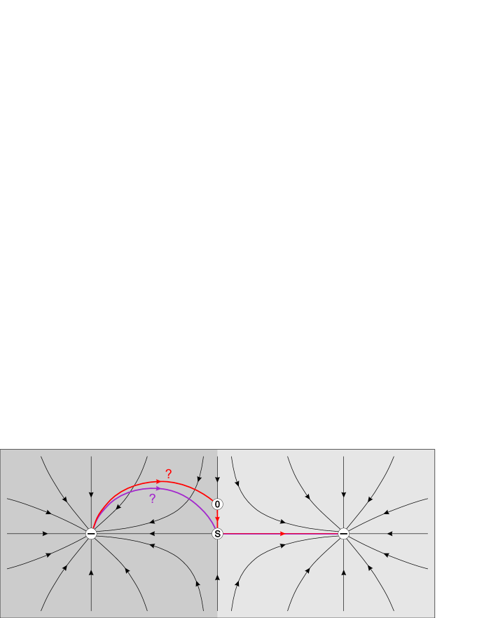
The answer to this question is given in Theorem 2. Note that in contrast to the previous chapter, here we do not make any assumptions on the eigenvalues of $\nabla b$ at the attractors or at the saddle point.

Theorem 2.

Let $S\in\mathcal{H}_{0}^{+}$, let $b$ be a natural drift, let $x_{1},x_{2}\in D$ be two distinct attractors of $b$, let the open sets $B_{1},B_{2}\subset D$ denote their basins of attraction, let $X:=\partial B_{1}\cap\partial B_{2}\cap D$ denote their separatrix, and assume that $X\subset\tilde{D}^{\circ}$. Let $A_{1},A_{2}\subset\tilde{D}$ be such that $A_{1}\subset B_{1}$ and $x_{2}\in A_{2}\subset B_{2}$.

If the minimization problem $P(A_{1},A_{2})$ has a weak solution $\gamma^{\star}\subset B_{1}\cup B_{2}\cup X$ then its first and last hitting point of $X$ are critical points.

Proof.

Let us denote the first and the last hitting points of $X$ by $z_{1}:=\varphi^{\star}(\alpha_{1})$ and $z_{2}:=\varphi^{\star}(\alpha_{2})$, where $\varphi^{\star}\in\tilde{C}(0,1)$ is a parameterization of $\gamma^{\star}\in\tilde{\Gamma}_{A_{1}}^{A_{2}}$ and

$$\alpha_{1}:=\min\hskip 2.2pt\!\big{\{}\alpha\in[0,1]\,\big{|}\,\varphi^{\star}(\alpha)\in X\big{\}}\ \in(0,1),$$

$$\alpha_{2}:=\max\!\big{\{}\alpha\in[0,1]\,\big{|}\,\varphi^{\star}(\alpha)\in X\big{\}}\ \in(0,1).$$

First hitting point: $X$ is closed in $D$ by definition, we have $X\subset\tilde{D}^{\circ}$ by assumption, and $X=\bar{B}_{1}\cap\bar{B}_{2}\cap D$ is flow-invariant since $\bar{B}_{1}\cap D$ and $\bar{B}_{2}\cap D$ are. Therefore, to conclude that $z_{1}$ is a critical point it is by Corollary 2 enough to show that the curve given by $\varphi^{\star}|_{[0,\alpha_{1}]}$ is a weak solution of the minimization problem $P(A_{1},X)$.

To do so, assume that there were a curve $\gamma_{1}\in\tilde{\Gamma}_{A_{1}}^{X}$ with $S(\gamma_{1})<S(\varphi^{\star}|_{[0,\alpha_{1}]})\leq S(\gamma^{\star})$. One could then obtain a contradiction by constructing a curve in $\tilde{\Gamma}_{A_{1}}^{A_{2}}$ with an action less than $S(\gamma^{\star})$, as follows: First follow $\gamma_{1}$ from $A_{1}$ to $X$, then move from the endpoint of $\gamma_{1}$ into $B_{2}$ along a line segment $\gamma_{2}$ so short that $S(\gamma_{1})+S(\gamma_{2})<S(\gamma^{\star})$ (using Assumption ($\tilde{D}$) and Lemma 4 (ii)), and finally follow the drift $b$ into $x_{2}\in A_{2}$ at no additional cost (using Lemma 17 (iii)).

Last hitting point: To make the arguments at the beginning of this section rigorous, first we argue that $s:=S(\varphi^{\star}|_{[\alpha_{2},1]})=0$. Indeed, if $s$ were positive then in contradiction to the minimizing property of $\gamma^{\star}$ we could construct a curve in $\tilde{\Gamma}_{A_{1}}^{A_{2}}$ with an action less than $S(\gamma^{\star})$, as follows: First move along the curve segment given by $\varphi^{\star}|_{[0,\alpha_{2}+\delta]}$, where $\delta>0$ is chosen so small that $S(\varphi^{\star}|_{[\alpha_{2},\alpha_{2}+\delta]})<s$ and thus $S(\varphi^{\star}|_{[0,\alpha_{2}+\delta]})<S(\gamma^{\star})$; since $\varphi^{\star}(\alpha_{2}+\delta)\in B_{2}$ by definition of $\alpha_{2}$, we can then follow the drift from $\varphi^{\star}(\alpha_{2}+\delta)$ into $x_{2}\in A_{2}$ at no additional cost.

This shows that $s=0$, and we can conclude that $\ell(\varphi^{\star},{\varphi^{\star}}^{\prime})=0$ a.e. on $[\alpha_{2},1]$. Now if we had $b(z_{2})\neq 0$ and thus $b(\varphi^{\star})\neq 0$ on some interval $[\alpha_{2},\tilde{\alpha}]$, $\tilde{\alpha}>\alpha_{2}$, then Lemma 17 (i) would imply that ${\varphi^{\star}}^{\prime}=cb(\varphi^{\star})$ a.e. on $[\alpha_{2},\tilde{\alpha}]$ for some function $c(\alpha)\geq 0$, i.e. $\varphi^{\star}$ follows a flowline of $b$ on this interval. Since $\varphi^{\star}(\tilde{\alpha})\in B_{2}$ and $b(\varphi^{\star})\neq 0$ on $[\alpha_{2},\tilde{\alpha}]$, we would thus obtain the contradiction $z_{2}=\varphi^{\star}(\alpha_{2})\in B_{2}\subset D\setminus X$. ∎

5 Conclusions

We have defined the class $\mathcal{G}$ of geometric action functionals on the space $\Gamma$ of rectifiable curves (in fact on a larger space $\tilde{\Gamma}$ that contains also infinitely long curves), and we have shown that the Hamiltonian geometric actions that arose in [4, 5] in the context of large deviation theory belong to $\mathcal{G}$. We have extended the notion of a drift vector field $b$ from the large deviation geometric action of an SDE (1.3) to general actions $S\in\mathcal{G}$, such that any curve with vanishing action must be a flowline of $b$.

We developed conditions under which there exists a curve $\gamma^{\star}$ with

$$S(\gamma^{\star})=\inf_{\gamma\in\Gamma_{A_{1}}^{A_{2}}}S(\gamma),$$

i.e. a solution to the problem of minimizing some given action $S\in\mathcal{G}$ over all curves $\gamma$ leading from the set $A_{1}$ to the set $A_{2}$. The curve $\gamma^{\star}$ is called a strong solution if it has finite length, and it is called a weak solution if it passes certain critical points in infinite length. Using a compactness argument, we reduced this existence problem to a local property (“a point $x$ has local minimizers”), and we listed several criteria (whose proofs are the content of Parts II-III) with which one can check this property for a given point $x$, provided that the flowline diagram of an underlying drift is well-understood.

We then demonstrated in various examples how these criteria are oftentimes sufficient to show that every point in the state space has local minimizers. We also included some examples in which our criteria are insufficient, and we obtained some results that explain why. In particular, in one example we proved that no minimizer $\gamma^{\star}$ exists.

Finally, we showed various properties of geometric actions and their minimizers. Our main result here was that for certain actions, minimum action curves leading from one attractor of the drift to another reach and leave the separatrix between the two basins of attraction at a point with zero drift. In particular, this result applies to maximum likelihood transition curves in large deviation theory.

Future Work, Open Problems.

In a short follow-up paper the author will further investigate the drift $b$ in Fig. 9 (a) and prove the existence of a “minimizing spiral” leading from the attractor to the limit cycle. In the case of the drift in Fig. 9 (b) a minimizer will exist, too, but it is not clear whether it will be in the form of a curve $\gamma\in\tilde{\Gamma}$ that ends in one of the saddle points, or again in the form of a minimizing spiral. To answer this question, one will need new ideas to decide whether the points on the chain of flowlines have local minimizers.

Another interesting open question is whether it is possible to extend the criterion for strong local minimizers in Proposition 4 (ii) also to dimensions $n>2$. While it would certainly suffice to extend Lemma 27 (vi)-(vii) correspondingly, after several failed attempts the author now believes that Lemma 27 (vi) is false in higher dimensions, and so a change in strategy may be necessary. One possible alternative approach may be to omit the line (2.48) in the proof of Proposition 4 and instead use a generalized version of Lemma 26 that directly applies to our function $F$; in this way one would need to control the gradients $\nabla f_{i}$ only where $F=f_{i}$.

Appendix A Proofs of some Lemmas

A.1 Proof of Lemma 3

Proof.

Let $(\gamma_{n})_{n\in\mathbb{N}}\subset\tilde{\Gamma}(x)$ be given with the properties stated, and let $s_{0}:=\liminf_{n\to\infty}S(\gamma_{n})$. In a first step, let us pass on to a subsequence (which we again denote by $(\gamma_{n})_{n\in\mathbb{N}}$), such that $\lim_{n\to\infty}S(\gamma_{n})=s_{0}$ (we will only need this property for the proof of Lemma 5 (ii)). Let $(\tilde{\varphi}_{n})_{n\in\mathbb{N}}\subset\tilde{C}(x)$ be a corresponding sequence of parameterizations.

To facilitate the proof of Proposition 4 in Section 2.6, which will build on the construction of the present proof, let us rewrite our assumption (2.3) more generally as

$$\forall n\in\mathbb{N}\ \forall u>0\colon\ \int_{\gamma_{n}}\mathds{1}_{F(z)>u}\,|dz|\leq\eta(u),$$ (A.1)

where $F(w):=|w-x|$ for $\forall w\in D$. We point out that the only properties of $F$ that we will use are that (i) $F$ is continuous on $D$, and (ii) $\exists c>0$ $\forall w\in K\colon\ F(w)\geq c|w-x|$.

To begin, we first pick for $\forall n\in\mathbb{N}$ a value $\alpha_{\min}^{n}\in[0,1]$ such that $F(\tilde{\varphi}_{n}(\alpha_{\min}^{n}))=\min_{\alpha\in[0,1]}F(\tilde{\varphi}_{n}(\alpha))$. Since $\tilde{\varphi}_{n}\subset K$ for $\forall n\in\mathbb{N}$, we may (by passing on to a subsequence if necessary) assume that $\lim_{n\to\infty}\tilde{\varphi}_{n}(\alpha_{\min}^{n})$ exists. Next we define for $\forall k\in\mathbb{N}_{0}$

$$d_{k}^{-} :=\tfrac{1}{2}-2^{-(k+1)}, d_{k}^{+} :=\tfrac{1}{2}+2^{-(k+1)},$$

$$Q_{k}^{-} :=[d_{k}^{-},d_{k+1}^{-}], Q_{k}^{+} :=[d_{k+1}^{+},d_{k}^{+}],$$

$$Q_{k}^{\pm} :=Q_{k}^{-}\cup Q_{k}^{+}, J_{k} :=\textstyle\bigcup_{i=0}^{k}Q_{i}^{\pm}=[0,d_{k+1}^{-}]\cup[d_{k+1}^{+},1],$$

we choose a strictly decreasing sequence $(u_{k})_{k\in\mathbb{N}_{0}}\subset(0,\infty)$ such that

$$u_{0}\geq\max\!\Big{\{}\sup_{n\in\mathbb{N}}F(\tilde{\varphi}_{n}(0)),\ \sup_{n\in\mathbb{N}}F(\tilde{\varphi}_{n}(1))\Big{\}}$$ (A.2)

(this is possible since the right-hand side is bounded by $\max_{w\in K}F(w)$) and that $u_{k}\searrow 0$ as $k\to\infty$, and we define for $\forall n\in\mathbb{N}$ and $\forall k\in\mathbb{N}_{0}$ the compact set

$$I_{n,k}:=\big{\{}\alpha\in[0,1]\,\big{|}\,F\big{(}\tilde{\varphi}_{n}(\alpha)\big{)}\leq u_{k}\big{\}}.$$

Then we define for $\forall n\in\mathbb{N}$ the surjective, weakly increasing function$\alpha_{n}\colon[0,1]\to[0,1]$ as follows: At the points $d_{k}^{-}$ and $d_{k}^{+}$ we set

$$\alpha_{n}(d_{k}^{-}):=\begin{cases}\min I_{n,k}&\text{if $I_{n,k}\neq\varnothing$,}\\ \alpha_{\min}^{n}&\text{else},\end{cases}\qquad\alpha_{n}(d_{k}^{+}):=\begin{cases}\max I_{n,k}&\text{if $I_{n,k}\neq\varnothing$,}\\ \alpha_{\min}^{n}&\text{else},\end{cases}$$ (A.3)

for $\forall k\in\mathbb{N}_{0}$, and we set $\alpha_{n}(\frac{1}{2}):=\alpha_{\min}^{n}$.

Before we define $\alpha_{n}(s)$ at the remaining points $s\in[0,1]$, observe that $\alpha_{n}(0)=0$ and $\alpha_{n}(1)=1$, since (A.2) implies that $0,1\in I_{n,0}$. Also note that every function $\alpha_{n}$ as defined so far is non-decreasing since for each fixed $n\in\mathbb{N}$ the sequence of sets $(I_{n,k})_{k\in\mathbb{N}_{0}}$ is decreasing, and since $\alpha_{\min}^{n}\in I_{n,k}$ whenever $I_{n,k}\neq\varnothing$ (which implies that $\alpha_{n}(d_{k}^{-})\leq\alpha_{\min}^{n}\leq\alpha_{n}(d_{k}^{+})$for $\forall k\in\mathbb{N}_{0}$).

Finally, observe that for $\forall k\in\mathbb{N}$ and $\forall n\in\mathbb{N}$ we have

either $$\forall\alpha\in[0,\alpha_{n}(d_{k}^{-})]\colon\,\ F(\tilde{\varphi}_{n}(\alpha))\geq u_{k}$$ (A.4a)

or $$\alpha_{n}(d_{k}^{-})=0$$ (A.4b)

(or both), and the same is true with $[0,\alpha_{n}(d_{k}^{-})]$ replaced by $[\alpha_{n}(d_{k}^{+}),1]$ in (A.4a), and with (A.4b) replaced by $\alpha_{n}(d_{k}^{+})=1$. Indeed, if $\alpha_{n}(d_{k}^{-})>0$ then for $\forall\alpha\in[0,\alpha_{n}(d_{k}^{-}))$ we have $\alpha\notin I_{n,k}$, i.e. $F(\tilde{\varphi}_{n}(\alpha))>u_{k}$, which implies (A.4a). The modified statement is shown analogously.

In either case, the curve segments given by $\tilde{\varphi}_{n}|_{[0,\alpha_{n}(d_{k}^{-})]}$ are rectifiable for $\forall k\in\mathbb{N}$: If (A.4a) holds then this follows from (A.1) with $u=\frac{u_{k}}{2}$, and if (A.4b) holds then this segment degenerates to a single point. Similarly, the segments given by $\tilde{\varphi}_{n}|_{[\alpha_{n}(d_{k}^{+}),1]}$ are rectifiable for $\forall k\in\mathbb{N}$ by the corresponding modified versions of (A.4a)-(A.4b).

We can thus define $\alpha_{n}(s)$ at the remaining points $s\in[0,1]$ by requiring that the function $\varphi_{n}(s):=\tilde{\varphi}_{n}(\alpha_{n}(s))$, restricted to the sets $Q_{k}^{-}$ and $Q_{k}^{+}$, $k\in\mathbb{N}_{0}$, is the arclength parameterization of the curves given by $\tilde{\varphi}_{n}|_{[\alpha_{n}(d_{k}^{-}),\alpha_{n}(d_{k+1}^{-})]}$ and $\tilde{\varphi}_{n}|_{[\alpha_{n}(d_{k+1}^{+}),\alpha_{n}(d_{k}^{+})]}$, respectively. In particular, on each set $Q_{k}^{-}$ and $Q_{k}^{+}$, $\varphi_{n}$ is absolutely continuous and $|\varphi_{n}^{\prime}|$ is constant a.e..

By construction, $\varphi_{n}|_{[0,\frac{1}{2}]}$ and $\varphi_{n}|_{[\frac{1}{2},1]}$ traverse the curves given by $\tilde{\varphi}_{n}|_{[0,\hat{\alpha}_{n}]}$ and $\tilde{\varphi}_{n}|_{[\check{\alpha}_{n},1]}$, where $\hat{\alpha}_{n}:=\lim_{k\to\infty}\alpha_{n}(d_{k}^{-})$ and $\check{\alpha}_{n}=\lim_{k\to\infty}\alpha_{n}(d_{k}^{-})$ (these limits exist since $(\alpha_{n}(d_{k}^{-}))_{k\in\mathbb{N}_{0}}$ and $(\alpha_{n}(d_{k}^{+}))_{k\in\mathbb{N}_{0}}$ are monotone bounded sequences). Therefore, to see that $\varphi_{n}$ is in fact a parameterization of the entire curve $\gamma_{n}$, we need to show that $\tilde{\varphi}_{n}$ is constant on $[\hat{\alpha}_{n},\check{\alpha}_{n}]$.

Now if (for fixed $n\in\mathbb{N}$) there $\exists k_{0}\in\mathbb{N}_{0}\ \forall k\geq k_{0}\colon\ I_{n,k}=\varnothing$ then we have $\forall k\geq k_{0}\colon\ \alpha_{n}(d_{k}^{-})=\alpha_{\min}^{n}=\alpha_{n}(d_{k}^{+})$ and thus $\hat{\alpha}_{n}=\check{\alpha}_{n}$, and we are done. Otherwise we have $\alpha_{n}(d_{k}^{-})\in I_{n,k}$ for $\forall k\in\mathbb{N}_{0}$, and thus $F\big{(}\tilde{\varphi}_{n}(\alpha_{n}(d_{k}^{-}))\big{)}\leq u_{k}\to 0$ as $k\to\infty$. This shows that $F(\tilde{\varphi}_{n}(\hat{\alpha}_{n}))=0$ and thus $\tilde{\varphi}_{n}(\hat{\alpha}_{n})=x$, and similarly one can show that $\tilde{\varphi}_{n}(\check{\alpha}_{n})=x$. Because of our assumption that $\gamma_{n}$ passes the point $x$ at most once we can now use (2.2) to conclude that $\tilde{\varphi}_{n}$ is constant on $[\hat{\alpha}_{n},\check{\alpha}_{n}]$ also in this case.

This shows that $\varphi_{n}$ is a parameterization of $\gamma_{n}$ (and in particular continuous). Furthermore, we have $\varphi_{n}\in\tilde{C}(x)$. To see this, first note that by construction $\varphi_{n}$ is absolutely continuous on $[0,\frac{1}{2}-a]\cup[\frac{1}{2}+a,1]$ for $\forall a\in(0,\frac{1}{2})$. If $\varphi_{n}(\frac{1}{2})\neq x$ then $F(\tilde{\varphi}_{n}(\alpha_{\min}))=F(\varphi_{n}(\frac{1}{2}))>0$, so that for large $k\in\mathbb{N}$ we have $I_{n,k}=\varnothing$ and thus $\alpha_{n}(d_{k}^{-})=\alpha_{n}(d_{k}^{+})$ by (A.3); this in turn implies that $\alpha_{n}$ and thus $\varphi_{n}$ is constant on $[d_{k}^{-},d_{k}^{+}]$, and thus that $\varphi_{n}\in\bar{C}({0,1})$.
Now let us construct a converging subsequence of $(\varphi_{n})_{n\in\mathbb{N}}$. First observe that our definition $\varphi_{n}=\tilde{\varphi}_{n}\circ\alpha_{n}$ and the monotonicity of $\alpha_{n}$ translate (A.4a)-(A.4b) into the following: For $\forall k\in\mathbb{N}$ and $\forall n\in\mathbb{N}$ we have

either $$\forall s\in[0,d_{k}^{-}]\colon\,\ F(\varphi_{n}(s))\geq u_{k}$$ (A.5a)

or $$\varphi_{n} [0,d_{k}^{-}]$$ is constant on (A.5b)

(or both), and the same is true with $[0,d_{k}^{-}]$ replaced by $[d_{k}^{+},1]$.

We can now find a subsequence of functions $\varphi_{n}$ that for $k=1$ either all fulfill (A.5a) or that all fulfill (A.5b); we can then find a further subsubsequence such that the same is true for $k=2$, etc., and by a diagonalization argument we can pass on to a subsequence which we again denote by $(\varphi_{n})_{n\in\mathbb{N}}$ such that for $\forall k\in\mathbb{N}$ $\exists n_{k}\in\mathbb{N}$ such that

$$\begin{split}\text{either}\hskip 19.91684pt&\forall n\geq n_{k}\,\ \forall s\in[0,d_{k}^{-}]\colon\,\ F(\varphi_{n}(s))\geq u_{k}\\ \text{or}\hskip 36.98866pt&\forall n\geq n_{k}\colon\,\ \text{$\varphi_{n}$ is constant on $[0,d_{k}^{-}]$}\end{split}$$ (A.6)

(or both). Finally, by following the same strategy one more time we may also assume that the same is true also with $[0,d_{k}^{-}]$ replaced by $[d_{k}^{+},1]$. This property (A.6) is not important to us now, but we will need it in the proof of Proposition 4.

Now using that for $\forall n\in\mathbb{N}$, $|\varphi_{n}^{\prime}|$ is constant a.e. on the intervals $Q_{k}^{-}$ and $Q_{k}^{+}$, and using (A.5a) and (A.5b), which say that either $|\varphi_{n}^{\prime}|$ vanishes a.e. on $[0,d_{k+1}^{-}]\supset Q_{k}^{-}$ or the indicator function in (A.7) below takes the value $1$ on $[0,d_{k+1}^{-}]\supset Q_{k}^{-}$, we find for $\forall k\in\mathbb{N}_{0}$ and almost every $s\in Q_{k}^{-}$ that

$$|\varphi_{n}^{\prime}(s)| =|Q_{k}^{-}|^{-1}\int_{Q_{k}^{-}}|\varphi_{n}^{\prime}|\,d\alpha=(2^{-(k+2)})^{-1}\int_{Q_{k}^{-}}|\varphi_{n}^{\prime}|\mathds{1}_{F(\varphi_{n})\geq u_{k+1}}\,d\alpha$$ (A.7)

$$\leq 2^{k+2}\int_{0}^{1}|\varphi_{n}^{\prime}|\mathds{1}_{F(\varphi_{n})>u_{k+2}}\,d\alpha\leq 2^{k+2}\eta(u_{k+2}),$$

and analogously one can derive this $n$-independent upper bound also for almost every $s\in Q_{k}^{+}$. This shows that for every fixed $k\in\mathbb{N}_{0}$ we have

$$\sup_{n\in\mathbb{N}}\,\operatorname*{ess\,sup}_{s\in J_{k}}|\varphi_{n}^{\prime}(s)|=\sup_{0\leq j\leq k}\,\sup_{n\in\mathbb{N}}\,\operatorname*{ess\,sup}_{s\in Q_{j}^{\pm}}|\varphi_{n}^{\prime}(s)|\leq\sup_{0\leq j\leq k}2^{j+2}\eta(u_{j+2})<\infty.$$ (A.8)

By Lemma 2 (i) we can therefore extract a subsequence of $(\varphi_{n})_{n\in\mathbb{N}}$ that converges uniformly on $J_{1}$, then extract a further subsubsequence converging uniformly on $J_{2}$, etc., and using a diagonalization argument we can find a subsequence which for simplicity we will again denote by $(\varphi_{n})_{n\in\mathbb{N}}$ that converges uniformly on every $J_{k}$, and in particular pointwise on $\bigcup_{k=0}^{\infty}J_{k}=[0,\frac{1}{2})\cup(\frac{1}{2},1]$. Since also $\varphi_{n}(\frac{1}{2})=\tilde{\varphi}_{n}\big{(}\alpha_{\min}^{n}\big{)}$ converges as $n\to\infty$, $(\varphi_{n})_{n\in\mathbb{N}}$ converges in fact pointwise on all of $[0,1]$. Let us denote the limit by $\varphi:[0,1]\to K$.
By Lemma 2 (ii) the function $\varphi$ is absolutely continuous on each set $J_{k}$, which provides us with an almost everywhere defined function ${\varphi}^{\prime}\colon[0,1]\to\mathbb{R}^{n}$ which is integrable on each set $J_{k}$. To see that

$$\int_{0}^{1}|{\varphi}^{\prime}|\mathds{1}_{F(\varphi)>u}\,d\alpha\leq\eta(u)\qquad\text{ for $\forall u>0$,}$$ (A.9)

we fix $u>0$, and we define for $\forall v>u$ and $\forall q\in\mathbb{R}$ the continuous function $h_{v}(q):=\min(\max(\frac{q-u}{v-u},0),1)\leq\mathds{1}_{q>u}$. Applying Lemma 5 (i) to the functional $S\in\mathcal{G}$ given by $\ell(x,y):=h_{v}(F(x))|y|$, we find that for $\forall k\in\mathbb{N}$ we have

$$\int_{J_{k}}h_{v}(F(\varphi))|{\varphi}^{\prime}|\,d\alpha \leq\liminf_{n\to\infty}\int_{J_{k}}h_{v}(F(\varphi_{n}))|\varphi_{n}^{\prime}|\,d\alpha$$

$$\leq\liminf_{n\to\infty}\int_{0}^{1}\mathds{1}_{F(\varphi_{n})>u}|\varphi_{n}^{\prime}|\,d\alpha$$

$$=\liminf_{n\to\infty}\int_{\gamma_{n}}\mathds{1}_{F(z)>u}\,|dz|\leq\eta(u)$$

by (A.1). Taking the limits $k\to\infty$ and $v\searrow u$ and using monotone convergence now imply (A.9).
It remains to show that $\varphi\in\tilde{C}(x)$. To prepare, let us first show that for $\forall k\in\mathbb{N}_{0}$ we have

either $$F(\varphi(d_{k}^{-}))\leq u_{k}$$ (A.10a)

or $$\varphi [d_{k}^{-},\tfrac{1}{2}]$$ is constant on (A.10b)

(or both), and the same holds with $d_{k}^{-}$ replaced by $d_{k}^{+}$ in (A.10a), and with $[d_{k}^{-},\tfrac{1}{2}]$ replaced by $[\tfrac{1}{2},d_{k}^{+}]$ in (A.10b).

Indeed, if for some fixed $k\in\mathbb{N}_{0}$ we have $F(\varphi(d_{k}^{-}))>u_{k}$ then for large $n\in\mathbb{N}$ we have $F\big{(}\tilde{\varphi}_{n}(\alpha_{n}(d_{k}^{-}))\big{)}=F(\varphi_{n}(d_{k}^{-}))>u_{k}$, i.e. $\alpha_{n}(d_{k}^{-})\notin I_{n,k}$ and thus $\alpha_{n}(d_{k}^{-})=\alpha_{\min}^{n}=\alpha_{n}(\tfrac{1}{2})$ by (A.3). The monotonicity of $\alpha_{n}$ then implies for large $n\in\mathbb{N}$ that $\alpha_{n}$ and thus $\varphi_{n}$ are constant on $[d_{k}^{-},\tfrac{1}{2}]$, and taking the limit $n\to\infty$ implies (A.10b). The modified statements can be shown analogously.

Next, let us show that $\varphi$ is continuous. Since $\varphi$ is even absolutely continuous on every set $J_{k}$, we only have to show continuity at $s=\tfrac{1}{2}$, and by symmetry of our construction we only have to show that $\varphi(\tfrac{1}{2}-)=\varphi(\tfrac{1}{2})$. Now if for some $k\in\mathbb{N}$ (A.10b) holds then this is clear, therefore let us assume that (A.10a) holds for $\forall k\in\mathbb{N}$. Taking the limit $k\to\infty$ in (A.10a) implies that $\liminf_{s\nearrow 1/2}F(\varphi(s))=0$. Thus, if the limit $\lim_{s\nearrow 1/2}F(\varphi(s))$ would not exist then there would be a sequence $(s_{m})_{m\in\mathbb{N}}\in(0,\frac{1}{2})$ with $s_{m}\nearrow\frac{1}{2}$ such that for some $u>0$ and $\forall m\in\mathbb{N}$ we have $F(\varphi(s_{m}))\geq 2u$. Now $F^{-1}([0,u])\cap K$ is compact, so that

$$\operatorname*{dist}\!\Big{(}F^{-1}([0,u])\cap K,\ F^{-1}([2u,\infty))\Big{)}>0,$$

and thus the fact that $\varphi(s)$ moves back and forth between these two sets infinitely many times as $s\nearrow\frac{1}{2}$ would imply that $\int_{0}^{1/2}|{\varphi}^{\prime}|\mathds{1}_{u<F(\varphi)<2u}\,d\alpha$ $=\infty$, contradicting (A.9). This proves that $\lim_{s\nearrow 1/2}F(\varphi(s))=0$, and since by construction $F\circ\varphi$ takes its minimum at $s=\frac{1}{2}$, we have $F(\varphi(\frac{1}{2}))=0$. Property (ii) of $F$ now implies that $\lim_{s\nearrow 1/2}\varphi(s)=x=\varphi(\frac{1}{2})$, concluding the proof of the continuity of $\varphi$.

Finally, to show that $\varphi\in\tilde{C}(x)$, assume that $\varphi(\frac{1}{2})\neq x$. Then neither (A.10a) nor its modified version can hold for $\forall k\in\mathbb{N}$ (since taking the limit $k\to\infty$ in (A.10a) would imply that $F(\varphi(\frac{1}{2}))=0$ and thus $\varphi(\frac{1}{2})=x$), and so $\varphi$ must be constant on some interval $[d_{k_{1}}^{-},d_{k_{2}}^{+}]$. Since $\varphi$ is absolutely continuous on every set $J_{k}$, this implies that $\varphi\in\bar{C}({0,1})$, terminating the proof. ∎

A.2 Proof of Lemma 5

Proof.

(i) Denoting by $M>0$ the bound given in (2.1), it suffices to define a family of functions $\ell^{\delta}\colon D\times\bar{B}_{M}(0)\to[0,\infty)$, $\delta>0$, such that
(a) $\forall\delta>0$ $\forall x\in D$ $\forall y\in\bar{B}_{M}(0)\colon$ $0\leq\ell^{\delta}(x,y)\leq\inf_{w\in\bar{B}_{\delta}(x)\cap D}\ell(w,y)$, (b) $\forall\delta>0$ $\forall x\in D\colon$ $\ell^{\delta}(x,\cdot\,)$ is convex, (c) $\forall x_{0}\in D$ $\forall y_{0}\in\bar{B}_{M}(0)\colon$ $\liminf_{(x,y,\delta)\to(x_{0},y_{0},0+)}\ell^{\delta}(x,y)\geq\ell(x_{0},y_{0})$.
The proof then follows the lines of [3, Lemma 5.42] (where the distance function induced by the norm $||\cdot||_{\infty}$ is denoted by $d_{c}$). The only necessary modification of that proof is that because of the property in Definition 1 (i) we do not have an equivalent to [3, Lemmas 5.17 and 5.18], and so we had to guarantee the uniform absolute continuity of the sequence $(\varphi_{n})_{n\in\mathbb{N}}$ by requiring the uniform bound on $|\varphi_{n}^{\prime}|$ in (2.1). That same bound is also the reason why (other than in [3]) here it suffices to define the functions $\ell^{\delta}(x,y)$ only for $|y|\leq M$.

To do so, we define for $\forall\delta>0$, $\forall x\in D$ and $\forall y\in\bar{B}_{M}(0)$

$$\ell^{\delta}(x,y) :=\sup_{(\theta,a)\in\Theta_{x,\delta}}\big{[}{\langle\theta,y\rangle}+a\big{]},\quad\text{where}$$

$$\Theta_{x,\delta} :=\Big{\{}(\theta,a)\in\mathbb{R}^{n}\times\mathbb{R}\ \Big{|}\ \forall v\in\bar{B}_{M}(0)\colon\,{\langle\theta,v\rangle}+a\leq\inf_{w\in\bar{B}_{\delta}(x)\cap D}\ell(w,v)\Big{\}},$$

i.e. $\ell^{\delta}(x,\cdot\,)$ is the convex hull of the function $v\mapsto\inf_{w\in\bar{B}_{\delta}(x)\cap D}\ell(w,v)$ restricted to $v\in\bar{B}_{M}(0)$.

(a,b) First observe that $(\theta,a)=(0,0)$ fulfills ${\langle\theta,v\rangle}+a=0\leq\ell(w,v)$ for every $w$ and $v$, and so we have $(0,0)\in\Theta_{x,\delta}$ and thus $\ell^{\delta}(x,y)\geq{\langle 0,y\rangle}+0=0$. The upper bound in (a) follows right from the definition of $\ell^{\delta}(x,y)$ and $\Theta_{x,\delta}$. Finally, $\ell^{\delta}(x,\cdot\,)$ is convex as the supremum over affine functions.

(c) Let $x_{0}\in D$ and $y_{0}\in\bar{B}_{M}(0)$. If $\ell(x_{0},y_{0})=0$ then by the lower bound in part (a) there is nothing to prove, therefore let us assume that $\ell(x_{0},y_{0})>0$. Since $\ell(x_{0},\cdot\,)$ is convex, $\exists\theta\in\mathbb{R}^{n}\ \exists a\in\mathbb{R}$ such that

$$\ell(x_{0},y_{0})={\langle\theta,y_{0}\rangle}+a\quad\text{and}\quad\forall y\in\mathbb{R}^{n}\colon\ \ell(x_{0},y)\geq{\langle\theta,y\rangle}+a.$$

In particular, for $\forall c\geq 0$ we can apply the latter to $y=cy_{0}$ to find that $c{\langle\theta,y_{0}\rangle}+a\leq c\ell(x_{0},y_{0})=c({\langle\theta,y_{0}\rangle}+a)$ and thus $(1-c)a\leq 0$. This shows that $a=0$, and so we have

$$\ell(x_{0},y_{0})={\langle\theta,y_{0}\rangle}\quad\text{and}\quad\forall y\in\mathbb{R}^{n}\colon\ \ell(x_{0},y)-{\langle\theta,y\rangle}\geq 0.$$ (A.11)

Given any $\varepsilon>0$, there thus $\exists\eta>0$ such that

$$\forall w\in\bar{B}_{\eta}(x_{0})\ \forall v\in\bar{B}_{M}(0)\colon\ \ell(w,v)-{\langle\theta,v\rangle}\geq-\varepsilon.$$ (A.12)

Now let $(x,y,\delta)\in\bar{B}_{\eta/2}(x_{0})\times\bar{B}_{M}(0)\times(0,\tfrac{\eta}{2})$. Since for $\forall w\in\bar{B}_{\delta}(x)\cap D$ we have $w\in\bar{B}_{\eta}(x_{0})$, (A.12) implies that $(\theta,-\varepsilon)\in\Theta_{x,\delta}$, so that

$$\ell^{\delta}(x,y) \geq{\langle\theta,y\rangle}-\varepsilon$$

$$={\langle\theta,y_{0}\rangle}+{\langle\theta,y-y_{0}\rangle}-\varepsilon$$

$$=\ell(x_{0},y_{0})+{\langle\theta,y-y_{0}\rangle}-\varepsilon$$

$$\geq\ell(x_{0},y_{0})-|\theta||y-y_{0}|-\varepsilon.$$

by the first statement of (A.11). This shows that

$$\liminf_{(x,y,\delta)\to(x_{0},y_{0},0+)}\ell^{\delta}(x,y)\geq\ell(x_{0},y_{0})-\varepsilon,$$

and since $\varepsilon>0$ was arbitrary, the proof of property (c) and thus of Lemma 5 (i) is complete.
(ii) Since the convergence is uniform on each set $I_{a}:=[0,\frac{1}{2}-a]\cup[\frac{1}{2}+a,1]$, $a\in(0,\frac{1}{2})$, and since (2.1) is fulfilled for the sequences $\big{(}\varphi_{n_{k}}|_{I_{a}}\big{)}_{k\in\mathbb{N}}$ by (A.8), Lemma 5 (i) allows us to estimate the combined action of the two pieces of the function $\varphi|_{I_{a}}$ by

$$\int_{I_{a}}\ell(\varphi,{\varphi}^{\prime})\,d\alpha=S(\varphi|_{I_{a}})\leq\liminf_{k\to\infty}S(\varphi_{n_{k}}|_{I_{a}})\leq\liminf_{k\to\infty}S(\gamma_{n_{k}})=\liminf_{n\to\infty}S(\gamma_{n}).$$

In the last step we used that at the beginning of the proof of Lemma 3 we had made sure that $\lim_{k\to\infty}S(\gamma_{n_{k}})=\liminf_{n\to\infty}S(\gamma_{n})$. Letting $a\searrow 0$ and then using the monotone convergence theorem now imply that

$$S(\gamma)=\int_{0}^{1}\ell(\varphi,{\varphi}^{\prime})\,d\alpha\leq\liminf_{n\to\infty}S(\gamma_{n}).\qed$$

A.3 Proof of Lemma 7

Proof.

(i) If (2.10) holds for some $H$ then the function $H(x,\cdot\,)$, which is strictly convex by Assumption (H3), achieves its minimum value $0$ at the point $\theta=0$, implying that $\{\theta\in\mathbb{R}^{n}\,|\,H(x,\theta)\leq 0\}=\{0\}$ and thus $\ell(x,y)=0$ for $\forall y\in\mathbb{R}^{n}$. Conversely, if $\forall y\in\mathbb{R}^{n}\colon\ \ell(x,y)=0$ and $H$ is any Hamiltonian inducing $S$ then we have $\forall\theta\neq 0\colon\ H(x,\theta)>0$ (for if there were a $\theta\neq 0$ with $H(x,\theta)\leq 0$ then we had $\ell(x,y=\theta)\geq{\langle\theta,\theta\rangle}>0$), and so by Assumption (H1) $H(x,\cdot\,)$ achieves its minimum value $0$ at the point $\theta=0$, which implies (2.10).
(ii) Let $x\in D$. By Assumption (H1) we have $H(x,0)\leq 0$. If $H(x,0)<0$ then given any $y\neq 0$ we have $H(x,\theta=\varepsilon y)<0$ for some small $\varepsilon>0$, and thus $\ell(x,y)\geq{\langle y,\varepsilon y\rangle}>0$. Now assume that $H(x,0)=0$. If $x$ is a critical point then we have $\ell(x,y)$ $=0$ even for $\forall y\in\mathbb{R}^{n}$. Otherwise by part (i) we have $y:=H_{\theta}(x,0)\neq 0$, and since for $\forall\theta\in\mathbb{R}^{n}$ with $H(x,\theta)\leq 0$ there $\exists\tilde{\theta}\in\mathbb{R}^{n}$ such that

$$0\geq H(x,\theta)=H(x,0)+{\langle H_{\theta}(x,0),\theta\rangle}+\tfrac{1}{2}{\big{\langle}\theta,H_{\theta\theta}(x,\tilde{\theta})\theta\big{\rangle}}\geq 0+{\langle y,\theta\rangle}+0$$

by Assumption (H3), we find that $\ell(x,y)\leq 0$ and thus $\ell(x,y)=0$. ∎

A.4 Proof of Lemma 8

Proof.

First let us show the existence of a solution of (2.11). If $x$ is a critical point then $(\vartheta,\lambda)=(0,0)$ solves (2.11) for $\forall y\in\mathbb{R}^{n}$ by Lemma 7 (i) (this also shows the first direction of part (ii)). If $x$ is not critical then we have $H_{\theta}(x,\theta)\neq 0$ whenever $H(x,\theta)=0$ (for otherwise $H(x,\cdot\,)$ would take its minimum value $0$ at $\theta$, and since the minimizer is unique by Assumption (H3), Assumption (H1) would imply that $\theta=0$, i.e. $x$ is a critical point by Lemma 7 (i)). Thus, for fixed $y\neq 0$, any $\theta^{\star}\in\mathbb{R}^{n}$ that is a solution the constraint maximization problem (2.8b) (and thus also of (2.8a)) must solve $\nabla_{\!\theta,\mu}\big{[}{\langle y,\theta\rangle}-\mu H(x,\theta)\big{]}=0$ for some $\mu\in\mathbb{R}$, i.e.

$$y=\mu H_{\theta}(x,\theta^{\star})\qquad\text{and}\qquad H(x,\theta^{\star})=0.$$

Clearly, $\mu\neq 0$ since $y\neq 0$. In fact, $\mu>0$ since otherwise we would have ${\langle H_{\theta}(x,\theta^{\star}),y\rangle}=|y|^{2}/\mu<0$ and thus $H(x,\theta^{\star}+\varepsilon y)<0$ for some $\varepsilon>0$, but then ${\langle y,\theta^{\star}+\varepsilon y\rangle}>{\langle y,\theta^{\star}\rangle}$ would contradict the fact that $\theta^{\star}$ is a maximizer of (2.8a). Therefore $(\vartheta,\lambda):=(\theta^{\star},\mu^{-1})$ solves (2.11).

Next we will show the uniqueness, and that the representation (2.12), which is trivial for $y=0$, holds also for $y\neq 0$. Let $x\in D$ and $y\in\mathbb{R}^{n}\setminus\{0\}$, and let $(\vartheta,\lambda)$ be a solution of (2.11). Since $\lambda=|H_{\theta}(x,\vartheta)|/|y|$, the uniqueness of $(\vartheta,\lambda)$ will follow from the uniqueness of $\vartheta$.

If $\lambda=0$ then (2.11) says that $H(x,\cdot\,)$ takes its minimum value $0$ at $\vartheta$, and thus again by Assumptions (H1) and (H3) we must have $\vartheta=0$ (proving uniqueness). By Lemma 7 (i), (2.11) now says that $x$ is a critical point, so (2.12) returns the correct value $\ell(x,y)=0$. This also shows the reverse direction of part (ii).

If $\lambda>0$ then for $\forall\theta\in L_{x}:=\{\theta\in\mathbb{R}^{n}\,|\,H(x,\theta)\leq 0\}$ there $\exists\tilde{\theta}\in\mathbb{R}^{n}$ such that by (2.11) and Assumption (H3) we have

$$0\geq H(x,\theta) =H(x,\vartheta)+{\langle H_{\theta}(x,\vartheta),\theta-\vartheta\rangle}+\tfrac{1}{2}{\big{\langle}\theta-\vartheta,H_{\theta\theta}(x,\tilde{\theta})(\theta-\vartheta)\big{\rangle}}$$

$$\geq 0+\lambda{\langle y,\theta-\vartheta\rangle}+\tfrac{1}{2}m_{\{x\}}|\theta-\vartheta|^{2}$$

$$\Rightarrow\hskip 19.91684pt{\langle y,\vartheta\rangle} \geq{\langle y,\theta\rangle}+\tfrac{1}{2}m_{\{x\}}\lambda^{-1}|\theta-\vartheta|^{2}\geq{\langle y,\theta\rangle}.$$ (A.13)

Since also $\vartheta\in L_{x}$, this implies that $\ell(x,y)={\langle y,\vartheta\rangle}$, i.e. (2.12). If $(\vartheta^{\prime},\lambda^{\prime})$ is another solution of (2.11) then we have ${\langle y,\vartheta\rangle}=\ell(x,y)={\langle y,\vartheta^{\prime}\rangle}$, and so setting $\theta:=\vartheta^{\prime}$ in the left inequality in (A.13) implies that $\vartheta=\vartheta^{\prime}$.

Finally, to show the continuity, suppose that for some $(x,y)\in D\times(\mathbb{R}^{n}\setminus\{0\})$ there exists a sequence $(x_{n},y_{n})\to(x,y)$ such that $(\vartheta_{n},\lambda_{n}):=(\vartheta(x_{n},y_{n}),\lambda(x_{n},y_{n}))$ stays bounded away from $(\vartheta(x,y),\lambda(x,y))$. Since $\vartheta_{n}\in L_{x_{n}}$ and the sets $L_{x_{n}}$ are uniformly bounded by what was shown at the beginning of the proof of Lemma 6, the sequence $(\vartheta_{n})$ is bounded. Thus, since $\lambda_{n}=|H_{\theta}(x_{n},\vartheta_{n})|/|y_{n}|$, also the sequence $(\lambda_{n})$ is bounded, and so there is a converging subsequence $(\vartheta_{n_{k}},\lambda_{n_{k}})$. Now letting $k\to\infty$ in the system (2.11) for $(x_{n_{k}},y_{n_{k}})$ and using the uniqueness shown above, we see that its limit must be $(\vartheta(x,y),\lambda(x,y))$, and we obtain a contradiction. ∎

A.5 Proof of Lemma 15 (ii)

Proof.

“$\Leftarrow$”: If (3.8) holds then choosing $w=x$ implies that $x$ is a critical point by Definition 4.
“$\Rightarrow$”: If $x$ is a critical point then it fulfills (2.10), and so by our assumption there $\exists a,\delta,\rho>0$ such that for $\forall w\in K:=\bar{B}_{\rho}(x)\subset D$ we have $|H(w,0)|\leq a|w-x|^{2\delta}$ and $|H_{\theta}(w,0)|\leq a|w-x|^{2\delta}$. Because of (2.9) the second equation in (2.11) implies that $c:=\sup_{w\in K,\,y\in\mathbb{R}^{n}}|\vartheta(w,y)|<\infty$. Finally, let $m_{K}>0$ be the constant given by Assumption (H3), and let $c_{4}:=(2a(1+c)m_{K}^{-1})^{1/2}$.

Now let $w\in\bar{B}_{\rho}(x)$ and $y\in\mathbb{R}^{n}$. If $y=0$ then $\ell(x,y)=0$ and there is nothing to prove. Otherwise we abbreviate $\vartheta:=\vartheta(w,y)$, and a Taylor expansion gives us a $\tilde{\theta}\in\mathbb{R}^{n}$ such that

$$0=H(w,\vartheta) =H(w,0)+{\big{\langle}H_{\theta}(w,0),\vartheta\big{\rangle}}+\tfrac{1}{2}{\big{\langle}\vartheta,H_{\theta\theta}(w,\tilde{\theta})\vartheta\big{\rangle}}$$

$$\geq-a|w-x|^{2\delta}-a|w-x|^{2\delta}\,|\vartheta|+\tfrac{1}{2}m_{K}|\vartheta|^{2}$$

$$\geq-a(1+c)|w-x|^{2\delta}+\tfrac{1}{2}m_{K}|\vartheta|^{2}$$

$$\Longrightarrow\hskip 48.36958pt|\vartheta| \leq\big{(}2a(1+c)m_{K}^{-1}\big{)}^{\!1/2}\,|w-x|^{\delta}=c_{4}|w-x|^{\delta}.\hskip 22.76228pt$$

The estimate (3.8) thus follows from (2.12). ∎

A.6 Proof of Lemma 18

Proof.

For greater transparency, we will first lead the proof for the special case of the local action (1.7).
SDE case. Let $B\subset D$ be a closed ball around $x$ that is so small that $d_{1}:=\min_{w\in B}|b(w)|$ $>0$, and further define $d_{2}:=\max_{w\in B}|b(w)|$ and $d_{3}:=\max_{w\in B}|\nabla b(w)|$. Let $\tilde{\alpha}\in[0,1)$ be so large that $\varphi|_{[\tilde{\alpha},1]}\subset B$, and define for $\alpha\in[\tilde{\alpha},1]$

$$\eta(\alpha):=\big{|}\widehat{\varphi^{\prime}}-\widehat{b(\varphi)}\big{|}^{2}=2\big{(}1-{\big{\langle}\widehat{\varphi^{\prime}},\widehat{b(\varphi)}\big{\rangle}}\big{)},$$

where we use the notation $\hat{w}=\frac{w}{|w|}$ for $\forall w\in\mathbb{R}^{n}\setminus\{0\}$. Note that $\eta(\alpha)$ is well-defined a.e. on $[\tilde{\alpha},1]$ because $b(\varphi)\neq 0$ on $[\tilde{\alpha},1]$ (by our choice of $B$ and $\tilde{\alpha}$), and because $|{\varphi}^{\prime}|\equiv\operatorname*{length}(\gamma)>0$ a.e. on $[0,1]$.

First we claim that there are arbitrarily large values $\alpha_{0}\in[\tilde{\alpha},1)$ such that $\int_{\alpha_{0}}^{1}\eta(\alpha)\,d\alpha>0$. Indeed, if this were not true then there would exist an $\alpha_{0}\in[\tilde{\alpha},1)$ such that $\eta=0$ and thus $\widehat{\varphi^{\prime}}=\widehat{b(\varphi)}$ a.e. on $[\alpha_{0},1]$. But this would mean that on $[\alpha_{0},1]$, $\varphi$ traverses a flowline of $b$ that ends in $x$, and so we have $\varphi(\alpha)\in\psi(x,(-\tau,0])$ for $\forall$ sufficiently large $\alpha\in[0,1)$, contradicting (4.1).

We pick $\alpha_{0}<1$ so large that $d_{2}d_{3}\operatorname*{length}(\gamma)(1-\alpha_{0})\leq\frac{1}{4}d_{1}^{2}$ and formally compute

$$\partial_{\varepsilon}S(\gamma_{\varepsilon})|_{\varepsilon=0} =\lim_{\varepsilon\to 0}\tfrac{1}{\varepsilon}\int_{0}^{1}\big{[}\ell(\varphi_{\varepsilon},\varphi_{\varepsilon}^{\prime})-\ell(\varphi,\varphi^{\prime})\big{]}\,d\alpha$$

$$=\lim_{\varepsilon\to 0}\int_{\alpha_{0}}^{1}\tfrac{1}{\varepsilon}\big{[}\ell(\varphi_{\varepsilon},\varphi_{\varepsilon}^{\prime})-\ell(\varphi,\varphi^{\prime})\big{]}\,d\alpha$$

$$=\int_{\alpha_{0}}^{1}\partial_{\varepsilon}\ell(\varphi_{\varepsilon},\varphi_{\varepsilon}^{\prime})|_{\varepsilon=0}\,d\alpha.$$ (A.14)

The last step of exchanging limit and integral will be justified rigorously when we treat the general case. Since

$$\varphi_{\varepsilon}^{\prime}=\varphi^{\prime}+\varepsilon\big{(}b(\varphi)+(\alpha-\alpha_{0})\nabla b(\varphi)\varphi^{\prime}\big{)},$$

a.e. on $[\alpha_{0},1]$, the integrand of (A.14) is

$$\partial_{\varepsilon}\ell(\varphi_{\varepsilon},\varphi_{\varepsilon}^{\prime})|_{\varepsilon=0}=\, \partial_{\varepsilon}\big{(}|b(\varphi_{\varepsilon})|\,|\varphi_{\varepsilon}^{\prime}|-{\langle b(\varphi_{\varepsilon}),\varphi_{\varepsilon}^{\prime}\rangle}\big{)}\big{|}_{\varepsilon=0}$$

$$=\, |\varphi^{\prime}|{\big{\langle}\widehat{b(\varphi)},\nabla b(\varphi)(\alpha-\alpha_{0})b(\varphi)\big{\rangle}}$$

$$+|b(\varphi)|{\big{\langle}\widehat{\varphi^{\prime}},b(\varphi)+(\alpha-\alpha_{0})\nabla b(\varphi)\varphi^{\prime}\big{\rangle}}$$

$$-{\big{\langle}{\varphi}^{\prime},\nabla b(\varphi)(\alpha-\alpha_{0})b(\varphi)\big{\rangle}}$$

$$-{\big{\langle}b(\varphi),b(\varphi)+(\alpha-\alpha_{0})\nabla b(\varphi)\varphi^{\prime}\big{\rangle}}$$

$$=\, -|b(\varphi)|^{2}\big{(}1-{\big{\langle}\widehat{\varphi^{\prime}},\widehat{b(\varphi)}\big{\rangle}}\big{)}$$

$$+(\alpha-\alpha_{0})|b(\varphi)|\,|\varphi^{\prime}|{\big{\langle}\widehat{b(\varphi)}-\widehat{\varphi^{\prime}},\nabla b(\varphi)\big{(}\widehat{b(\varphi)}-\widehat{\varphi^{\prime}}\big{)}\big{\rangle}}$$

$$\leq\, -\tfrac{1}{2}d_{1}^{2}\eta(\alpha)+d_{2}d_{3}(1-\alpha_{0})|\varphi^{\prime}|\big{|}\widehat{b(\varphi)}-\widehat{\varphi^{\prime}}\big{|}^{2}$$

$$=\, \eta(\alpha)\big{[}{-\tfrac{1}{2}}d_{1}^{2}+d_{2}d_{3}(1-\alpha_{0})\operatorname*{length}(\gamma)\big{]}$$

$$\leq\, -\tfrac{1}{4}d_{1}^{2}\eta(\alpha).$$

Plugging this into (A.14), we obtain

$$\partial_{\varepsilon}S(\gamma_{\varepsilon})|_{\varepsilon=0}\leq-\tfrac{1}{4}d_{1}^{2}\int_{\alpha_{0}}^{1}\eta(\alpha)\,d\alpha<0.$$

General case. We choose $B$ and $\tilde{\alpha}$ as before, but now we define $\eta(\alpha):=|\vartheta(\varphi,\varphi^{\prime})|^{2}$. Again, there are arbitrarily large $\alpha_{0}\in[\tilde{\alpha},1)$ with $\int_{\alpha_{0}}^{1}\eta(\alpha)\,d\alpha>0$ since $\,\eta(\alpha)=0\ \,\Rightarrow\ \,\vartheta(\varphi,\varphi^{\prime})=0\ \,\Rightarrow\ \,H_{\theta}(\varphi,0)=\lambda(\varphi,\varphi^{\prime})\varphi^{\prime}\ \,\Rightarrow\ \,\widehat{\varphi^{\prime}}=\widehat{H_{\theta}(\varphi,0)}=\widehat{b(\varphi)}$ (the second step followed from the definition (2.11) of $\vartheta(x,y)$, in the third step we used that $H_{\theta}(\varphi,0)\neq 0$ by our choice of $B$ and $\tilde{\alpha}$). By implicit differentiation in (2.11), [4, Appendix E] shows that for $\forall x\in D$ and $\forall y\neq 0$ we have

$$\vartheta_{x}(x,y)^{T}y =-\lambda^{-1}(x,y)H_{x}(x,\vartheta(x,y))\qquad\text{wherever\, $\lambda(x,y)\neq 0$,}$$

$$\vartheta_{y}(x,y)^{T}y =0.$$

From (2.12) we therefore obtain

$$\nabla_{\!x}\ell(x,y) = \vartheta_{x}^{T}(x,y)y=-\lambda^{-1}(x,y)H_{x}(x,\vartheta(x,y)),$$

$$\nabla_{\!y}\ell(x,y) = \vartheta_{y}^{T}(x,y)y+\vartheta(x,y)=\vartheta(x,y)$$

wherever $y\neq 0$ and $\lambda(x,y)\neq 0$, and thus, abbreviating $\vartheta_{\varepsilon}=\vartheta(\varphi_{\varepsilon},\varphi_{\varepsilon}^{\prime})$ and $\lambda_{\varepsilon}=\lambda(\varphi_{\varepsilon},\varphi_{\varepsilon}^{\prime})$, we have a.e. on $[\alpha_{0},1]$

$$\partial_{\varepsilon}\ell(\varphi_{\varepsilon},\varphi_{\varepsilon}^{\prime}) =-\lambda_{\varepsilon}^{-1}{\big{\langle}H_{x}(\varphi_{\varepsilon},\vartheta_{\varepsilon}),\partial_{\varepsilon}\varphi_{\varepsilon}\big{\rangle}}+{\big{\langle}\vartheta_{\varepsilon},\partial_{\varepsilon}\varphi_{\varepsilon}^{\prime}\big{\rangle}}$$

$$=-\lambda_{\varepsilon}^{-1}{\big{\langle}H_{x}(\varphi_{\varepsilon},\vartheta_{\varepsilon}),(\alpha-\alpha_{0})b(\varphi)\big{\rangle}}$$

$$\hskip 12.23447pt+{\big{\langle}\vartheta_{\varepsilon},b(\varphi)+(\alpha-\alpha_{0})\nabla b(\varphi)\varphi^{\prime}\big{\rangle}}$$ (A.15)

Setting $\varepsilon=0$ and abbreviating $\vartheta=\vartheta(\varphi,\varphi^{\prime})$ and $\lambda=\lambda(\varphi,\varphi^{\prime})$, we find

$$\partial_{\varepsilon}\ell(\varphi_{\varepsilon},\varphi_{\varepsilon}^{\prime})\big{|}_{\varepsilon=0}={\big{\langle}\vartheta,b(\varphi)\big{\rangle}}+(\alpha-\alpha_{0})\Big{[}{\big{\langle}\vartheta,\nabla b(\varphi)\varphi^{\prime}\big{\rangle}}-\lambda^{-1}{\big{\langle}H_{x}(\varphi,\vartheta),b(\varphi)\big{\rangle}}\Big{]}.$$ (A.16)

To show that the first term is negative, we make a Taylor expansion and find that for some $\tilde{\vartheta}$ we have

$$0=H(\varphi,\vartheta) =H(\varphi,0)+{\big{\langle}H_{\theta}(\varphi,0),\vartheta\big{\rangle}}+\tfrac{1}{2}{\big{\langle}\vartheta,H_{\theta\theta}(\varphi,\tilde{\vartheta})\vartheta\big{\rangle}}$$

$$\geq 0+{\langle b(\varphi),\vartheta\rangle}+\tfrac{1}{2}m_{B}|\vartheta|^{2}$$

$$\Rightarrow\quad{\langle\vartheta,b(\varphi)\rangle} \leq-\tfrac{1}{2}m_{B}|\vartheta|^{2},$$ (A.17)

where we used Assumptions (H1’) and (H3). To control the second term in (A.16), we make two more Taylor expansions and use the equations $H_{x}(x,0)$ $=0$ (a consequence of Assumption (H1’)) and (2.11) to show that

$$H_{x}(\varphi,\vartheta) =H_{x}(\varphi,0)+H_{x\theta}(\varphi,0)\vartheta+O(|\vartheta|^{2})=0+\nabla b(\varphi)^{T}\vartheta+O(|\vartheta|^{2}),$$

$$b(\varphi) =H_{\theta}(\varphi,0)=H_{\theta}(\varphi,\vartheta)+O(|\vartheta|)=\lambda\varphi^{\prime}+O(|\vartheta|).$$

Note that to bound the first remainder term we had to require the existence of a continuous derivative $H_{x\theta\theta}$, and we also needed a uniform bound on $\varphi$ (which is in $B$) and on $\vartheta$ (which then follows from what was shown at the beginning of the proof of Lemma 6). The square bracket term in (A.16) is thus

$$[\dots] ={\big{\langle}\vartheta,\nabla b(\varphi)\varphi^{\prime}\big{\rangle}}-\lambda^{-1}{\big{\langle}\nabla b(\varphi)^{T}\vartheta+O(|\vartheta|^{2}),\lambda\varphi^{\prime}+O(|\vartheta|)\big{\rangle}}$$

$$=O(|\vartheta|^{2}),$$ (A.18)

where we used that $\lambda^{-1}$ is bounded. (The latter follows from Lemma 8 (ii) and the continuity of $\lambda$, since $\varphi$ is in the compact set $B$ which does not contain any critical points, and since $|\varphi^{\prime}|\equiv\operatorname*{length}(\gamma)>0$ a.e..) Now combining (A.16), (A.17) and (A.18), and choosing $\alpha_{0}$ sufficiently close to $1$, we find that

$$\partial_{\varepsilon}\ell(\varphi_{\varepsilon},\varphi_{\varepsilon}^{\prime})\big{|}_{\varepsilon=0}\leq-\tfrac{1}{2}m_{B}|\vartheta|^{2}+(1-\alpha_{0})\cdot\tilde{c}|\vartheta|^{2}\leq-c|\vartheta|^{2}=-c\eta(\alpha)$$

for some constants $\tilde{c},c>0$, and thus $\partial_{\varepsilon}S(\gamma_{\varepsilon})|_{\varepsilon=0}\leq-c\int_{\alpha_{0}}^{1}\eta(\alpha)\,d\alpha<0$.

It remains to justify the exchange of limit and integral in (A.14). Using the mean value theorem and Lebesgue, this boils down to finding a bound on (A.15) that is uniform in both $\varepsilon>0$ and $\alpha\in[\alpha_{0},1]$. But this is a straight forward estimate since $\vartheta_{\varepsilon}$ and $\lambda_{\varepsilon}^{-1}$ are uniformly bounded in $\alpha$ and $\varepsilon$ (for reasons similar to the ones used for $\vartheta$ and $\lambda^{-1}$ above). ∎

Part II Proofs

2 Finding Points with Local Minimizers

2.1 Proof of Proposition 2

The key to the proof of Proposition 2 is that the condition $\forall y\neq 0\colon\!\!$$\ell(x,y)>0$ implies that we can locally estimate $|y|\leq\frac{1}{\mu}\ell(x,y)$ for some $\mu>0$, which in turn will provide us with a quick way to locally bound the length of a curve by its action. Since minimizing sequences have bounded actions, their lengths must therefore be bounded as well, and we can apply Proposition 1.

Proof of Proposition 2.

We will prove the stronger condition of Remark 2 (ii). Let $\eta>0$ be given. Since $\min_{|y|=1}\ell(x,y)>0$, there exists an $\varepsilon>0$ such that $\bar{B}_{\varepsilon}(x)\subset D$ and

$$\mu:=\min_{\begin{subarray}{c}w\in\bar{B}_{\varepsilon}(x)\\ |y|=1\end{subarray}}\ell(w,y)>0.$$

Using Definition 1 (i), this implies that

$$\forall w\in\bar{B}_{\varepsilon}(x)\ \forall y\neq 0\colon\ \ \ell(w,y)=|y|\ell\big{(}w,\tfrac{y}{|y|}\big{)}\geq\mu|y|,$$ (2.1)

and for $y=0$ this relation is trivial. Let $c_{1}=c_{1}(\bar{B}_{\varepsilon}(x))>0$ be the constant given by Lemma 4 (ii), let $\nu:=\min\!\big{\{}\varepsilon,\frac{\mu\varepsilon}{5c_{1}},\frac{\eta\mu}{2c_{1}}\big{\}}$, and finally use Assumption ($\tilde{D}$) to choose $r\in(0,\tfrac{1}{2}\varepsilon]$ so small that for $\forall w\in\bar{B}_{r}(x)\cap\tilde{D}$ $\exists\gamma\in\Gamma_{x}^{w}$: $\operatorname*{length}(\gamma)\leq\nu$.

Now let $x_{1},x_{2}\in\bar{B}_{r}(x)\cap\tilde{D}$. For $i=1,2$ let $\bar{\gamma}^{i}\in\Gamma^{x_{i}}_{x}$ with $\operatorname*{length}(\bar{\gamma}^{i})\leq\nu$ and thus in particular $\bar{\gamma}^{i}\subset\bar{B}_{\nu}(x)\subset\bar{B}_{\varepsilon}(x)$, and let $\bar{\gamma}:=-\bar{\gamma}^{1}+\bar{\gamma}^{2}\in\Gamma_{x_{1}}^{x_{2}}$. Since $\bar{\gamma}\subset\bar{B}_{\varepsilon}(x)$, we can use Lemma 4 (ii) to find that

$$\inf_{\gamma\in\Gamma_{x_{1}}^{x_{2}}}S(\gamma)\leq S(\bar{\gamma})\leq c_{1}\operatorname*{length}(\bar{\gamma})\leq 2c_{1}\nu.$$ (2.2)

Next, let $(\varphi_{n})_{n\in\mathbb{N}}\subset\bar{C}_{x_{1}}^{x_{2}}(0,1)$ be a parameterization of a minimizing sequence $(\gamma_{n})_{n\in\mathbb{N}}$ of $P(x_{1},x_{2})$. We claim that

$$\exists n_{0}\in\mathbb{N}\ \forall n\geq n_{0}\colon\ \gamma_{n}\subset\bar{B}_{\varepsilon}(x).$$ (2.3)

Indeed, if this were not the case then we could find a subsequence $(\varphi_{n_{k}})_{n\in\mathbb{N}}$ such that $\forall k\in\mathbb{N}\ \exists\alpha\in[0,1]\colon\ |\varphi_{n_{k}}(\alpha)-x|=\varepsilon$. Letting $\alpha_{k}:=$$\min\!\big{\{}\alpha\in[0,1]\,\big{|}\,|\varphi_{n_{k}}(\alpha)-x|\geq\varepsilon\big{\}}\in(0,1)$ and applying (2.1), we would then have

$$S(\gamma_{n_{k}}) \geq\int_{0}^{\alpha_{k}}\ell(\varphi_{n_{k}},\varphi_{n_{k}}^{\prime})\,d\alpha$$

$$\geq\mu\int_{0}^{\alpha_{k}}|\varphi_{n_{k}}^{\prime}|\,d\alpha$$

$$\geq\mu\bigg{|}\int_{0}^{\alpha_{k}}\varphi_{n_{k}}^{\prime}\,d\alpha\bigg{|}$$

$$=\mu|\varphi_{n_{k}}(\alpha_{k})-\varphi_{n_{k}}(0)|$$

$$=\mu\big{|}\big{(}\varphi_{n_{k}}(\alpha_{k})-x\big{)}+(x-x_{1})\big{|}$$

$$\geq\mu\big{(}|\varphi_{n_{k}}(\alpha_{k})-x|-|x-x_{1}|\big{)}$$

$$\geq\mu(\varepsilon-r)\geq\tfrac{1}{2}\mu\varepsilon.$$ (2.4)

Taking the limit $k\to\infty$ and using the minimizing property of $(\gamma_{n})_{n\in\mathbb{N}}$ and (2.2), we would thus find that $\frac{1}{2}\mu\varepsilon\leq 2c_{1}\nu$, which contradicts our definition of $\nu$. This proves (2.3), which allows us for $\forall n\geq n_{0}$ to apply (2.1) on the entire curve $\gamma_{n}$, and so we find that we have

$$S(\gamma_{n})=\int_{0}^{1}\ell(\varphi_{n},\varphi_{n}^{\prime})\,d\alpha\geq\mu\int_{0}^{1}|\varphi_{n}^{\prime}|\,d\alpha=\mu\cdot\operatorname*{length}(\gamma_{n})$$ (2.5)

for $\forall n\geq n_{0}$, and thus

$$\sup_{n\geq n_{0}}\operatorname*{length}(\gamma_{n})\leq\frac{1}{\mu}\sup_{n\geq n_{0}}S(\gamma_{n})<\infty.$$

We can now apply Proposition 1 and conclude that the problem $P(x_{1},x_{2})$ has a strong minimizer $\gamma^{\star}\in\Gamma_{x_{1}}^{x_{2}}$ fulfilling

$$\operatorname*{length}(\gamma^{\star}) \leq\liminf_{n\to\infty}\operatorname*{length}(\gamma_{n})\leq\frac{1}{\mu}\liminf_{n\to\infty}S(\gamma_{n})=\frac{1}{\mu}\inf_{\gamma\in\Gamma_{x_{1}}^{x_{2}}}S(\gamma)\leq\frac{2c_{1}\nu}{\mu}\leq\eta,$$

where we used (2.5), the minimizing property of $(\gamma_{n})_{n\in\mathbb{N}}$, (2.2), and the definition of $\nu$. ∎

2.2 Proof of Lemma 14

To prepare for the proof of Lemma 14 we first need to collect some properties of the functions $f_{s}$ and $f_{u}$ of Definition 9.

Lemma 20.

The functions $f_{s}$ and $f_{u}$ of Definition 9 are finite-valued and continuous. Furthermore,
(i) $f_{s}\in C^{1}(B_{s}\setminus\{x\})$ and $f_{u}\in C^{1}(B_{u}\setminus\{x\})$; (ii) $\displaystyle\forall w\in\hskip 0.7ptB_{s}\setminus\{x\}\colon\ \hskip 1.0pt{\langle\nabla f_{s}(w),b(w)\rangle}=$ $\displaystyle\!\!\!-\!$ $\displaystyle\!\!\!\!|b(w)|,$ (2.6a) $\displaystyle\forall w\in B_{u}\setminus\{x\}\colon\ {\langle\nabla f_{u}(w),b(w)\rangle}=$ $\displaystyle\!\!\!\!|b(w)|;$ (2.6b) (iii) $\displaystyle\forall w\in\hskip 0.7ptB_{s}\colon$ $\displaystyle f_{s}(w)\geq|w-x|,$ (2.7a) $\displaystyle\forall w\in B_{u}\colon$ $\displaystyle f_{u}(w)\geq|w-x|;$ (2.7b) (iv) $\displaystyle\forall\!\text{ compact }K\subset B_{s}\ \hskip 1.0pt\exists c_{5}\geq 1\ \forall w\in K\colon$ $\displaystyle f_{s}(w)$ $\displaystyle\!\!\!\leq c_{5}|w-x|,$ (2.8a) $\displaystyle\forall\!\text{ compact }K\subset B_{u}\ \exists c_{5}\geq 1\ \forall w\in K\colon$ $\displaystyle f_{u}(w)$ $\displaystyle\!\!\!\leq c_{5}|w-x|.$ (2.8b)

Proof.

See Appendix A. ∎

Proof of Lemma 14.

Let us assume first that $x$ is an unstable equilibrium point. Let $a>0$ be so small that $\bar{B}_{2a}(x)\subset B_{u}$, abbreviate $M:=M_{u}^{a}=f_{u}^{-1}(\{a\})$, and define

$$f_{M}(w):=\begin{cases}\min\{f_{u}(w)-a,a\}&\text{if $w\in B_{u}$,}\\ a&\text{else.}\end{cases}$$ (2.9)

Then $f_{M}$ is continuous on $D$. Indeed, $f_{u}$ is continuous on $B_{u}$, and for $\forall w\in B_{u}\setminus\bar{B}_{2a}(x)$ we have $f_{u}(w)\geq|w-x|>2a$ by (2.7b) and thus $f_{M}(w)=a$. It now remains to show the properties (i)-(iv) of Definition 8.
(i) $f_{M}(w)=0\ \Leftrightarrow\ \big{(}w\in B_{u}$ and $f_{u}(w)=a\big{)}\ \Leftrightarrow\ w\in f_{u}^{-1}(\{a\})=M$.
(ii) $M$ is closed as a level set of the continuous function $f_{M}$. $M$ is bounded since $M\subset\bar{B}_{a}(x)$: Indeed, if $w\in M$ then $|w-x|\leq f_{u}(w)=a$ by (2.7b).
(iii) Let $w_{0}\in M$, i.e. $f_{u}(w_{0})=a$. In particular, we must have $w_{0}\neq x$, since $f_{u}(x)=0$ by definition of $f_{u}$. Since $B_{u}$ is open, there exists an $\varepsilon>0$ such that $B_{\varepsilon}(w_{0})\subset B_{u}\setminus\{x\}$, and thus $f_{u}$ is $C^{1}$ on $B_{\varepsilon}(w_{0})$ by Lemma 20 (i). Since $f_{u}$ is continuous, we can also choose $\varepsilon>0$ so small that $\forall w\in B_{\varepsilon}(w_{0})\colon f_{u}(w)\in(\frac{a}{2},2a)$, which in particular implies that $f_{M}=f_{u}-a$ on $B_{\varepsilon}(w_{0})$, and thus that $f_{M}$ is $C^{1}$ on $B_{\varepsilon}(w_{0})$ as well. Since $w_{0}\in M$ was arbitrary, this shows that there exists a neighborhood of $M$ on which $f_{M}$ is $C_{1}$, with $\nabla f_{M}=\nabla f_{u}$.
(iv) Consequently, we have for $\forall w\in M$ that ${\langle\nabla f_{M}(w),b(w)\rangle}=$${\langle\nabla f_{u}(w),b(w)\rangle}=|b(w)|$ by (2.6b). Since $M\subset B_{u}\setminus\{x\}$ as seen in part (iii), we have for $\forall w\in M$ that $b(w)\neq 0$ and thus ${\langle\nabla f_{M}(w),b(w)\rangle}>0$.
If $x$ is a stable equilibrium point then the proof is carried out analogously, except that we replace $f_{u}$ by $f_{s}$ and then multiply the definition of $f_{M}$ by $-1$. In this way, in the proof of (iii) we will find that $\nabla f_{M}=-\nabla f_{s}$ on $M$, but since in the proof of part (iv) we will now have to use (2.6a) instead of (2.6b), we will still find that ${\langle\nabla f_{M}(w),b(w)\rangle}=-{\langle\nabla f_{s}(w),b(w)\rangle}=+|b(w)|>0$. ∎

2.3 Admissible Manifolds

In preparation for the proofs of Propositions 3 and 4, we will now collect some properties of admissible manifolds. Before proceeding, the reader is advised to review Definition 8 which we will soon use without further reference.

Lemma 21.

If $M$ is an admissible manifold then

$$\forall x\in M\ \,\forall t\in\mathbb{R}\colon\ \,\operatorname*{sgn}\!\big{(}f_{M}(\psi(x,t))\big{)}=\operatorname*{sgn}(t).$$ (2.10)

In particular, we have $\psi(x,t)\in M$ if and only if $t=0$, which shows that admissible manifolds cannot be crossed by the same flowline more than once.

Proof.

Let $x\in M$. Clearly, (2.10) holds for $t=0$ by Definition 8 (i). Suppose now that there were a $t>0$ such that $f_{M}(\psi(x,t))\leq 0$. Then

$$T:=\inf\!\big{\{}t>0\,\big{|}\,f_{M}(\psi(x,t))\leq 0\big{\}}$$

would be well-defined, and since

$$\partial_{t}f_{M}(\psi(x,t))\big{|}_{t=0}={\big{\langle}\nabla f_{M}(\psi(x,0)),\dot{\psi}(x,0)\big{\rangle}}={\langle\nabla f_{M}(x),b(x)\rangle}>0$$

by Definition 8 (iv), we would have $T>0$,

$$f_{M}(\psi(x,t))>0 \forall t\in(0,T)$$ for (2.11)

and $$w:=\psi(x,T)\in f_{M}^{-1}(\{0\})=M \psi(x,t)=\psi(w,t-T)$$. Since , (2.11) can be rewritten as

$$f_{M}(\psi(w,t))>0 \forall t\in(-T,0)$$ for .

But this would mean that

$${\langle\nabla f_{M}(w),b(w)\rangle} =\partial_{t}f_{M}(\psi(w,t))\big{|}_{t=0}$$

$$=\lim_{t\searrow 0}\tfrac{1}{t}\big{[}\underbrace{f_{M}(\psi(w,0))}_{=f_{M}(w)=0}-\underbrace{f_{M}(\psi(w,-t))}_{>0\ \text{for}\ t\in(0,T)}\big{]}\leq 0,$$

which contradicts property (iv) of Definition 8. Consequently, we must have $f_{M}(\psi(x,t))>0$ for $\forall t>0$, and with an analogous argument one can show that $f_{M}(\psi(x,t))<0$ for $\forall t<0$, concluding the proof of (2.10).

In particular, if a flowline crosses $M$ at some point $x$ then (2.10) implies that for $\forall t\neq 0$ we have $f_{M}(\psi(x,t))\neq 0$ and thus $\psi(x,t)\notin M$. ∎

Corollary 3.

If $x\in D$ lies on a limit cycle of $b$ then there is no admissible manifold $M$ with $x\in\psi(M,\mathbb{R})$.

Proof.

If $x\in D$ lies on a limit cycle then we have $\psi(x,T)=x$ for some $T>0$. If there existed an admissible manifold $M$, a $w\in M$ and a $t\in\mathbb{R}$ such that $\psi(w,t)=x$ then we would have $\psi(w,T)=\psi(x,T-t)=\psi(x,-t)=w\in M$, which contradicts Lemma 21. ∎

In particular, this shows that we cannot use Proposition 3 to prove that a given point on a limit cycle has local minimizers. Proposition 5 (ii) of Section 4.3 explains why this had to be the case: For actions $S\in\mathcal{H}_{0}^{+}$ points on limit cycles do not have local minimizers.

The next lemma (which is used in the proofs of Corollary 4 and Lemma 27) allows us to deform a given admissible manifold and turn it into a new one. With a smart choice of the function $\beta(x)$ this new manifold can have additional useful properties.

Definition 11.

For any $\beta\in C^{1}(D,\mathbb{R})$ we denote by $\psi_{\beta}\in C^{1}(D\times\mathbb{R},D)$ the flow corresponding to the vector field $\beta\cdot b$.

Lemma 22.

Let $\beta\in C^{1}(D,\mathbb{R})$. If $M$ is an admissible manifold and $T\in\mathbb{R}$ then also the set $M^{\prime}:=\psi_{\beta}(M,T)$ is an admissible manifold.

Proof.

We will show that the continuous function $f_{M^{\prime}}(x):=f_{M}(\psi_{\beta}(x,-T))$, $x\in D$, has the four properties of Definition 8.
(i) $f_{M^{\prime}}(x)=0$ $\ \,\Leftrightarrow\ \,$ $f_{M}(\psi_{\beta}(x,-T))=0$ $\ \,\Leftrightarrow\ \,$ $\psi_{\beta}(x,-T)\in M$ $\ \,\Leftrightarrow\ \,$ $x\in$$\psi_{\beta}(M,T)=M^{\prime}$.
(ii) $M^{\prime}=\psi_{\beta}(M,T)$ is compact as the continuous image of a compact set.
(iii) Denote by $N$ an open neighborhood of $M$ on which $f_{M}$ is $C^{1}$. Then $f_{M^{\prime}}(x)$ is $C^{1}$ wherever $\psi_{\beta}(x,-T)\in N$, i.e. where $x\in\psi_{\beta}(N,T)=:N^{\prime}\supset M^{\prime}$. Since $\psi_{\beta}(\,\cdot\,,T)$ has a continuous inverse (namely $\psi_{\beta}(\,\cdot\,,-T)$), $N^{\prime}$ is an open neighborhood of $M^{\prime}$.
(iv) Suppose that there exists an $x_{0}\in M^{\prime}$ such that ${\langle\nabla f_{M^{\prime}}(x_{0}),b(x_{0})\rangle}\leq 0$, and let $w:=\psi_{\beta}(x_{0},-T)\in M$. The functions

$$f_{t}(x):=f_{M}(\psi_{\beta}(x,-t)),\quad t\in\mathbb{R},\ x\in D,\$$

are $C^{1}$ in $(t,x)$ wherever $\psi_{\beta}(x,-t)\in N$, and thus in particular where $x=\psi_{\beta}(w,t)$. Therefore the function

$$g(t):={\big{\langle}\nabla f_{t}(\psi_{\beta}(w,t)),\,b(\psi_{\beta}(w,t))\big{\rangle}},\quad t\in\mathbb{R},$$

is well-defined and continuous, and since $f_{0}=f_{M}$ and $f_{T}=f_{M^{\prime}}$, it fulfills

$$g(0)={\langle\nabla f_{M}(w),b(w)\rangle}>0\qquad\text{and}\qquad g(T)={\langle\nabla f_{M^{\prime}}(x_{0}),b(x_{0})\rangle}\leq 0$$

(the first estimate is property (iv) of the admissible manifold $M$). This shows that $\exists t_{0}\in(0,T]\colon\ g(t_{0})=0$, and abbreviating $v:=\psi_{\beta}(w,t_{0})$, we find that

$$0 =\beta(v)g(t_{0})={\big{\langle}\nabla f_{t_{0}}(v),\beta(v)b(v)\big{\rangle}}=\partial_{\tau}f_{t_{0}}(\psi_{\beta}(v,\tau))\big{|}_{\tau=0}$$

$$=\partial_{\tau}f_{M}\big{(}\psi_{\beta}(v,\tau-t_{0})\big{)}\big{|}_{\tau=0}=\partial_{\tau}f_{M}(\psi_{\beta}(w,\tau))\big{|}_{\tau=0}$$

$$={\big{\langle}\nabla f_{M}(w),\beta(w)b(w)\big{\rangle}}=\beta(w)g(0)$$

and thus $\beta(w)=0$. In particular, this implies that

$$\psi_{\beta}(w,t)=w\quad\text{for $\forall t\in\mathbb{R}$,}$$ (2.12)

which enables us to compute an explicit formula for the function $h(t):=\nabla\psi_{\beta}(w,t)$: We have $h(0)=I$ (since $\psi_{\beta}(x,0)=x$ for $\forall x\in D$) and

$$\dot{h}(t) =\nabla_{\!\!x}\dot{\psi}_{\beta}(x,t)\big{|}_{x=w}=\nabla_{\!\!x}\big{[}(\beta b)(\psi_{\beta}(x,t))\big{]}\big{|}_{x=w}$$

$$=\big{(}\nabla(\beta b)\big{)}\big{(}\underbrace{\psi_{\beta}(w,t)}_{=w}\big{)}\underbrace{\nabla\psi_{\beta}(w,t)}_{=h(t)}=\big{(}\underbrace{\beta(w)}_{=0}\nabla b(w)+b(w)\otimes\nabla\beta(w)\big{)}h(t),$$

and so $\nabla\psi_{\beta}(w,t)=h(t)=\exp\!\big{(}b(w)\otimes t\nabla\beta(w)\big{)}$ for $\forall t\in\mathbb{R}$. Again using (2.12), we thus obtain the contradiction

$$g(t_{0}) ={\langle\nabla f_{t_{0}}(w),b(w)\rangle}$$

$$=\nabla f_{M}\big{(}\psi_{\beta}(w,-t_{0})\big{)}\nabla\psi_{\beta}(w,-t_{0})b(w)$$

$$=\nabla f_{M}(w)e^{b(w)\otimes(-t_{0})\nabla\beta(w)}b(w)$$

$$={\langle\nabla f_{M}(w),b(w)\rangle}e^{-t_{0}{\langle\nabla\beta(w),b(w)\rangle}}$$

$$>0.\qed$$

In other words, if one lets the points on $M$ follow the flow $\beta b$ for a fixed amount of time then one obtains a new admissible manifold. As a direct consequence we obtain Corollary 4, which in turn will reduce the proof of Proposition 3 to points $x\in M$ only.

Corollary 4.

If $x\in\psi(M,\mathbb{R})$ for some admissible manifold $M$ then there exists another admissible manifold $M^{\prime}$ such that $x\in M^{\prime}$.

Proof.

Let $x=\psi(w,T)$ for some $w\in M$ and some $T\in\mathbb{R}$ . Then $x\in M^{\prime}:=\psi(M,T)$, and by Lemma 22 (applied to $\beta:\equiv 1$) $M^{\prime}$ is an admissible manifold. ∎

The following lemma defines two functions $z(x)$ and $t(x)$ on the set $\psi(M,\mathbb{R})$ (that is the union of all the flowlines of $b$ emanating from $M$). These functions are used extensively throughout the rest of this paper, in particular in the proof of Lemma 27 to define a function $\beta$ for use in Lemma 22, and in the proofs of Lemmas 24 and 27 to define certain “flowline tracing functions” from admissible manifolds.

Lemma 23.

Let $M$ be an admissible manifold. Then $\psi(M,\mathbb{R})$ is open, and there exist two functions $z\in C^{1}(\psi(M,\mathbb{R}),M)$ and $t\in C^{1}(\psi(M,\mathbb{R}),\mathbb{R})$ whose values are the unique ones fulfilling

$$\forall x\in\psi(M,\mathbb{R})\colon\quad z(x)\in M\quad\text{and}\quad\psi(z(x),t(x))=x.$$ (2.13)

Furthermore, we have for $\forall x\in\psi(M,\mathbb{R})$

$$\nabla\!z(x)\,b(x) =0,$$ (2.14)

$${\langle\nabla t(x),b(x)\rangle} =1,$$ (2.15)

$$x\in M\quad\Leftrightarrow\quad t(x)=0\quad\Leftrightarrow\quad z(x)=x.$$ (2.16)

Proof.

Let us abbreviate $A:=\psi(M,\mathbb{R})$. The existence (but not the smoothness) of two functions $z(x)$ and $t(x)$ fulfilling $\psi(z(x),t(x))=x$ is clear by our choice of their domain $\psi(M,\mathbb{R})$. To show uniqueness, let $x\in A$, $z_{1},z_{2}\in M$ and $t_{1},t_{2}\in\mathbb{R}$ fulfill $\psi(z_{1},t_{1})=x=\psi(z_{2},t_{2})$. Then we have $\psi(z_{1},t_{1}-t_{2})=z_{2}\in M$, and Lemma 21 tells us that $t_{1}-t_{2}=0$, i.e. $t_{1}=t_{2}$. This in turn implies that $z_{2}=\psi(z_{1},t_{1}-t_{2})=\psi(z_{1},0)=z_{1}$.

To see that the functions $z$ and $t$ are $C^{1}$ on $A$, let $x\in A$. Let $\varepsilon>0$ be so small that $f_{M}$ is $C^{1}$ on $B_{\varepsilon}(z(x))$. Since $\psi(x,-t(x))=z(x)$, there exists a neighborhood $U$ of $(x,t(x))$ such that $\forall(w,\tau)\in U\colon\ \psi(w,-\tau)\in B_{\varepsilon}(z(x))$. In particular, the function $F(w,\tau):=f_{M}(\psi(w,-\tau))$ is $C^{1}$ on $U$. Since

$$F(x,t(x)) =f_{M}\big{(}\psi(x,-t(x))\big{)}=f_{M}(z(x))=0$$

$$\text{and}\quad\ \partial_{\tau}F(x,t(x)) =-{\big{\langle}\nabla f_{M}\big{(}\psi(x,-t(x))\big{)},\,b\big{(}\psi(x,-t(x))\big{)}\big{\rangle}}\hskip 28.45274pt$$

$$=-{\big{\langle}\nabla f_{M}(z(x)),b(z(x))\big{\rangle}}\neq 0$$

by Definition 8 (i) and (iv), we can apply the Implicit Function Theorem to obtain a $C^{1}$-function $\tilde{t}(w)$, defined in a neighborhood $V$ of $x$, such that for $\forall w\in V$ we have $0=F(w,\tilde{t}(w))=f_{M}\big{(}\psi(w,-\tilde{t}(w))\big{)}$, i.e. $\tilde{z}(w):=\psi(w,-\tilde{t}(w))\in M$. By definition of $\tilde{z}$ we have $\psi(\tilde{z}(w),\tilde{t}(w))=w$ for $\forall w\in V$, which tells us that (i) $V\subset A$, proving that $A$ is open, and (ii) $\tilde{t}=t|_{V}$ and $\tilde{z}=z|_{V}$ (because of the uniqueness of the functions $z$ and $t$). Since $\tilde{t}$ and $\tilde{z}$ are $C^{1}$, the latter shows that $t$ and $z$ are $C^{1}$ on $V$, and thus on all of $A$.

To show (2.14) and (2.15), we evolve both sides of (2.13) by some small time $\tau$ and find that $\psi\big{(}z(x),t(x)+\tau\big{)}=\psi(x,\tau)$, i.e.

$$z(\psi(x,\tau))=z(x)\qquad\text{and}\qquad t(\psi(x,\tau))=t(x)+\tau.$$

Differentiating with respect to $\tau$ and setting $\tau=0$, we obtain

$$0 =\nabla\!z(\psi(x,0))\,\dot{\psi}(x,0)=\nabla\!z(x)\,b(x)\hskip 36.98866pt\text{and}$$

$$1 ={\big{\langle}\nabla t(\psi(x,0)),\dot{\psi}(x,0)\big{\rangle}}={\langle\nabla t(x),b(x)\rangle}.$$

It remains to show (2.16). If $x\in M$ then the equation $\psi(x,0)=x$ and the uniqueness of the representation (2.13) imply that $t(x)=0$. If $t(x)=0$ then by (2.13) we have $x=\psi(z(x),0)=z(x)$. Finally, if $z(x)=x$ then $x\in M$ since $z$ takes values in $M$. ∎

With this new notation we can now rephrase Lemma 21 as follows.

Corollary 5.

Let $M$ be an admissible manifold, and let $t(x)$ be the corresponding function given by Lemma 23. Then we have

$$\forall x\in\psi(M,\mathbb{R})\ \,\forall t\in\mathbb{R}\colon\ \, \operatorname*{sgn}\!\big{(}f_{M}(\psi(x,t))\big{)}=\operatorname*{sgn}(t(x)+t),$$ (2.17)

$$\forall x\in\psi(M,\mathbb{R})\colon\ \, \operatorname*{sgn}(f_{M}(x))=\operatorname*{sgn}(t(x)).$$ (2.18)

Proof.

Using (2.13) we can write

$$\operatorname*{sgn}\!\big{(}f_{M}(\psi(x,t))\big{)}=\operatorname*{sgn}\!\big{(}f_{M}\big{(}\psi(z(x),t(x)+t)\big{)}\big{)},$$

and since $z(x)\in M$, we can apply Lemma 21 to obtain (2.17). To prove (2.18), set $t=0$. ∎

2.4 Flowline Tracing Functions

The purpose of this section is to find a replacement for the local bound $\ell(x,y)\geq\mu|y|$ that was used in (2.4) and (2.5) to bound the length of a curve in terms of its action. Without the condition of Proposition 2, our only lower bound on $\ell(x,y)$ is (2.6), which vanishes if $y=cb(x)$ for some $c\geq 0$. As a result, curves that follow the flowlines of $b$ could be arbitrarily long and have zero action. We thus need to exclude the possibility that the curve follows the flowlines of $b$ for arbitrarily long distances, for example because these flowlines lead far away from the desired endpoint.

To quantify this idea, consider for example the constant vector field $b(x)\equiv b_{0}\in\mathbb{R}^{n}\setminus\{0\}$. In this case, if $\gamma\subset K$ and if the start and end point of $\gamma$ are confined to a ball $\bar{B}_{r}(x)$ then we have

$$S(\gamma) =\int_{0}^{1}\ell(\varphi,\varphi^{\prime})\,d\alpha\geq c_{2}\int_{0}^{1}\big{(}|b_{0}||\varphi^{\prime}|-{\langle b_{0},\varphi^{\prime}\rangle}\big{)}\,d\alpha$$

$$=c_{2}\big{(}|b_{0}|\operatorname*{length}(\gamma)-{\langle b_{0},\varphi(1)-\varphi(0)\rangle}\big{)}$$

$$\Rightarrow\quad\operatorname*{length}(\gamma) =\tfrac{1}{c_{2}|b_{0}|}S(\gamma)+{\big{\langle}\tfrac{b_{0}}{|b_{0}|},\varphi(1)-\varphi(0)\big{\rangle}}\leq\tfrac{1}{c_{2}|b_{0}|}S(\gamma)+2r,$$ (2.19)

where $c_{2}=c_{2}(K)$, and again we have found a bound for the length of $\gamma$ in terms of its action.

For non-constant vector fields $b$ however, things are not that easy. We will have to lay out a non-cartesian coordinate grid that is compatible with this idea, i.e. one whose “$b$-coordinate” increases at unit speed along the flowlines of $b$. The manifold consisting of all the points with vanishing $b$-coordinate can be crossed by the flowlines of $b$ only in one direction, which leads us to the definition of admissible manifolds. The notion of such a coordinate grid is made precise by the following definition.

Definition 12.

A function $f\colon D\to\mathbb{R}$ is said to trace the flowlines of the vector field $b\colon D\to\mathbb{R}^{n}$ between the values $q_{1}$ and $q_{2}$ (for two real numbers $q_{1}<q_{2}$) if
(i) $f$ is continuous on $D$, (ii) $f$ is continuously differentiable on $E:=f^{-1}\big{(}(q_{1},q_{2})\big{)}$, (iii) we have either (iii.1) $\forall x\in E\colon\ {\langle\nabla f(x),b(x)\rangle}=|b(x)|$, or       (iii.2) $\forall x\in E\colon\ {\langle\nabla f(x),b(x)\rangle}=-|b(x)|.$

Property (iii) says that on the region $E$, $f$ increases or decreases at unit speed in the direction of the flow $b$, and thus for $x\in E$, $f(x)$ can be interpreted as the value of the $b$-coordinate of $x$. Note that if a function $f$ traces the flowlines of $b$ between $q_{1}$ and $q_{2}$ and if $(\tilde{q}_{1},\tilde{q}_{2})\subset(q_{1},q_{2})$, then $f$ also traces the flowlines of $b$ between $\tilde{q}_{1}$ and $\tilde{q}_{2}$.

The following lemma, which is used in the proof of Proposition 3, shows how to construct a flowline tracing function from an admissible manifold. A corresponding statement for Proposition 4 is given by Lemma 27.

Lemma 24.

Let $M$ be an admissible manifold. Then there exists an $\varepsilon>0$ and a function $f\in C(D,\mathbb{R})$ such that
(i) $f^{-1}(\{0\})=M$, (ii) $f$ traces the flowlines of $b$ between the values $-\varepsilon$ and $\varepsilon$, (iii) $\bar{E}$ is a compact subset of $D$, where $E:=f^{-1}\big{(}(-\varepsilon,\varepsilon)\big{)}$, (iv) $\forall\,x\in\bar{E}\colon\ \,b(x)\neq 0$, and (v) $\sup_{x\in E}|\nabla f(x)|<\infty$.

Proof.

Abbreviate $A:=\psi(M,\mathbb{R})$, let $z\in C^{1}(A,M)$ and $t\in C^{1}(A,\mathbb{R})$ be the functions given by Lemma 23, and define the function $g\in C^{1}(A,\mathbb{R})$ by

$$g(x):=\int_{0}^{t(x)}\big{|}b\big{(}\psi(z(x),\tau)\big{)}\big{|}\,d\tau\qquad\text{for $\forall x\in A$,}$$ (2.20)

i.e. $|g(x)|$ is the length of the flowline segment between $x$ and $z(x)$. First note that by Remark 5 we have $b(z(x))\neq 0$ and thus $b\big{(}\psi(z(x),\tau)\big{)}\neq 0$ for $\forall\tau\in\mathbb{R}$. This shows that $g$ is $C^{1}$ and (using (2.20) and (2.18)) that

$$\operatorname*{sgn}(g(x))=\operatorname*{sgn}(t(x))=\operatorname*{sgn}(f_{M}(x))\qquad\text{for $\forall x\in A$.}$$ (2.21)

Since $A$ is open by Lemma 23 and contains the compact set $M$, there $\exists\varepsilon>0$ such that $\bar{N}_{2\varepsilon}(M)\subset A$. Since for $\forall x\in G:=g^{-1}\big{(}(-2\varepsilon,2\varepsilon)\big{)}$ we have

$$|x-z(x)| =\big{|}\psi\big{(}z(x),t(x)\big{)}-\psi\big{(}z(x),0\big{)}\big{|}$$

$$=\bigg{|}\int_{0}^{t(x)}\dot{\psi}\big{(}z(x),\tau\big{)}\,d\tau\bigg{|}=\bigg{|}\int_{0}^{t(x)}b\big{(}\psi(z(x),\tau)\big{)}\,d\tau\bigg{|}$$

$$\leq\bigg{|}\int_{0}^{t(x)}\big{|}b\big{(}\psi(z(x),\tau)\big{)}\big{|}\,d\tau\bigg{|}=|g(x)|<2\varepsilon,$$

we have $G\subset\bar{N}_{2\varepsilon}(M)\subset A$. Finally, we set $D^{-}:=f_{M}^{-1}\big{(}(-\infty,0)\big{)}$ and $D^{+}:=f_{M}^{-1}\big{(}(0,\infty)\big{)}$, and we define the function $f\colon D\to\mathbb{R}$ as

$$f(x):=\begin{cases}g(x)&\text{if $x\in G$,}\\ -2\varepsilon&\text{if $x\in D^{-}\setminus G$,}\\ 2\varepsilon&\text{if $x\in D^{+}\setminus G$.}\end{cases}$$ (2.22)

Note that $f$ is well-defined since the three cases are defining $f$ on disjoint sets whose union is all of $D$. Indeed, since $f_{M}^{-1}(\{0\})=M\subset A$, (2.21) implies

$$f_{M}^{-1}(\{0\})=g^{-1}(\{0\})$$ (2.23)

and thus $D\setminus(D^{-}\cup D^{+})=f_{M}^{-1}(\{0\})=g^{-1}(\{0\})\subset G$. It remains to show that $f$ has the desired properties (i)-(v) of Lemma 24.

(i) Using (2.22)-(2.23) we find that $f^{-1}(\{0\})=g^{-1}(\{0\})=f_{M}^{-1}(\{0\})=M$.
(ii) To check that $f$ traces the flowlines of $b$ between the values $-\varepsilon$ and $\varepsilon$, we have to check the three properties of Definition 12:
(ii.1) For any set $B\subset D$ let us temporarily (i.e. for this part (ii.1) only) use the notation $\bar{B}$ to denote its closure in $D$. Clearly, $f$ is continuous on each of the three parts of the domain. To see that $f$ is also continuous on the boundaries of these regions, we use that $G$ is open, (2.23), (2.21), and that $\bar{G}\subset g^{-1}\big{(}[-2\varepsilon,2\varepsilon]\big{)}$ (since $\bar{G}\subset\bar{N}_{2\varepsilon}(M)\subset A$), to obtain

$$\overline{(D^{-}\setminus G)}\cap\overline{(D^{+}\setminus G)}\hskip 6.544pt =\hskip 6.544pt\big{(}\overline{D^{-}}\cap\overline{D^{+}}\big{)}\cap G^{c}$$

$$\subset\hskip 6.544ptf_{M}^{-1}\big{(}(-\infty,0]\big{)}\cap f_{M}^{-1}\big{(}[0,\infty)\big{)}\cap G^{c}$$

$$=\hskip 6.544ptf_{M}^{-1}(\{0\})\cap g^{-1}\big{(}(-2\varepsilon,2\varepsilon)\big{)}^{c}$$

$$\stackrel{{\scriptstyle\eqref{Dpm}}}{{=}}g^{-1}(\{0\})\cap g^{-1}\big{(}(-2\varepsilon,2\varepsilon)\big{)}^{c}=\varnothing,$$

$$\overline{(D^{-}\setminus G)}\cap\bar{G}\hskip 6.544pt =\hskip 6.544pt\overline{D^{-}}\cap G^{c}\cap\bar{G}$$

$$\subset\hskip 6.544ptf_{M}^{-1}\big{(}(-\infty,0]\big{)}\cap g^{-1}\big{(}(-2\varepsilon,2\varepsilon)\big{)}^{c}\cap g^{-1}\big{(}[-2\varepsilon,2\varepsilon]\big{)}$$

$$=\hskip 6.544ptf_{M}^{-1}\big{(}(-\infty,0]\big{)}\cap g^{-1}\big{(}\{-2\varepsilon,2\varepsilon\}\big{)}$$

$$\stackrel{{\scriptstyle\eqref{g t M}}}{{=}}g^{-1}(\{-2\varepsilon\}),\hskip 105.2751pt\text{and similarly}$$

$$\overline{(D^{+}\setminus G)}\cap\bar{G}\hskip 6.544pt \subset\hskip 6.544ptg^{-1}(\{2\varepsilon\}).$$

(ii.2) $f$ is $C^{1}$ on $G$ since $f|_{G}=g|_{G}$ and $g$ is $C^{1}$. Since $G=g^{-1}\big{(}(-2\varepsilon,2\varepsilon)\big{)}=f^{-1}\big{(}(-2\varepsilon,2\varepsilon)\big{)}\supset E$, this shows that $f$ is $C^{1}$ on $E$.
(ii.3) This also shows that for $\forall x\in G\supset E$ we have

$$\nabla f(x) =\nabla g(x)$$

$$=\big{|}b\big{(}\psi(z(x),t(x))\big{)}\big{|}\nabla t(x)$$

$$\hskip 36.98866pt{}+\int_{0}^{t(x)}\Big{(}\frac{b^{T}\nabla b}{|b|}\Big{)}\big{(}\psi(z(x),\tau)\big{)}\nabla\psi\big{(}z(x),\tau\big{)}\,d\tau\,\cdot\nabla\!z(x),$$

so (2.13)-(2.15) imply that ${\langle\nabla f(x),b(x)\rangle}=|b(x)|$.
(iii) The continuity of $f$ implies that $\bar{E}\subset f^{-1}\big{(}[-\varepsilon,\varepsilon]\big{)}=g^{-1}\big{(}[-\varepsilon,\varepsilon]\big{)}\subset G\subset\bar{N}_{2\varepsilon}(M)$. Since $\bar{N}_{2\varepsilon}(M)$ is compact, this shows that $\bar{E}$ is a compact subset of $G\subset D$.
(iv) This is a consequence of Remark 5 since $\bar{E}\subset G\subset A=\psi(M,\mathbb{R})$.
(v) This follows directly from our proofs of parts (ii.2) and (iii) where we showed that $f$ is $C^{1}$ on the set $G$ which contains the compact set $\bar{E}$. ∎

As we see, we cannot expect to cover all of $D$ with our grid, but only some set $E=f^{-1}((q_{1},q_{2}))$, and so our generalized version of the estimate (2.19), given in Lemma 26, must be restricted to $E$ as well. To do so, we need to introduce the continuous function $h_{q_{1}}^{q_{2}}$, which is equal to the identity on $[q_{1},q_{2}]$ and constant outside of $[q_{1},q_{2}]$. Two properties are given in Lemma 25.

Definition 13.

For any two real numbers $q_{1}<q_{2}$ we define the function $h_{q_{1}}^{q_{2}}\colon\mathbb{R}\to[q_{1},q_{2}]$ by

$$h_{q_{1}}^{q_{2}}(a):=\min\!\big{(}\!\max(a,q_{1}),q_{2}\big{)}.$$

Lemma 25.

For $\forall a_{1},a_{2}\in\mathbb{R}$ we have the estimates

$$\big{|}h_{q_{1}}^{q_{2}}(a_{1})-h_{q_{1}}^{q_{2}}(a_{2})\big{|} \leq q_{2}-q_{1},$$ (2.24a)

$$\big{|}h_{q_{1}}^{q_{2}}(a_{1})-h_{q_{1}}^{q_{2}}(a_{2})\big{|} \leq|a_{1}-a_{2}|.$$ (2.24b)

Proof.

The estimate (2.24a) holds because $h_{q_{1}}^{q_{2}}$ maps into $[q_{1},q_{2}]$, (2.24b) just says that $h_{q_{1}}^{q_{2}}$ is Lipschitz continuous with Lipschitz constant $1$, which can easily be checked by splitting $\mathbb{R}$ into $(-\infty,q_{1}]$, $[q_{1},q_{2}]$ and $[q_{2},\infty)$. ∎

Lemma 26.

Let $x_{1},x_{2}\in\tilde{D}$, $\gamma\in\Gamma_{x_{1}}^{x_{2}}$, $q_{1}<q_{2}$, let $f\colon D\to\mathbb{R}$ be a function that traces $b$ between the values $q_{1}$ and $q_{2}$, let $E:=f^{-1}\big{(}(q_{1},q_{2})\big{)}$, and assume that $\bar{E}$ is a compact subset of $D$. Let $c_{2}:=c_{2}(\bar{E})$ be the constant given by Definition 2, and assume that $c_{6}:=c_{6}(\bar{E}):=\min_{x\in\bar{E}}|b(x)|>0$ and $c_{7}:=c_{7}(f,q_{1},q_{2}):=\sup_{x\in E}|\nabla f(x)|<\infty$. Then we have

$$\operatorname*{length}\!\big{(}\gamma|_{f^{-1}((q_{1},q_{2}))}\big{)}\leq\frac{2c_{7}^{2}}{c_{2}c_{6}}S(\gamma)+2\big{|}h_{q_{1}}^{q_{2}}(f(x_{1}))-h_{q_{1}}^{q_{2}}(f(x_{2}))\big{|}.$$ (2.25)

Proof.

Let us abbreviate $L:=\operatorname*{length}(\gamma|_{E})$ and $\Delta:=h_{q_{1}}^{q_{2}}(f(x_{2}))-h_{q_{1}}^{q_{2}}(f(x_{1}))$. If $L-|\Delta|\leq 0$ then

$$L-2|\Delta|\leq 2(L-|\Delta|)\leq 0\leq\frac{2c_{7}^{2}}{c_{2}c_{6}}S(\gamma),$$

so (2.25) is clear. Therefore let us now assume that $L-|\Delta|>0$ and thus in particular $L>0$. Let $\varphi\in\bar{C}_{x_{1}}^{x_{2}}(0,1)$ be a parameterization of $\gamma$, and let

$$Q:=\big{\{}\alpha\in[0,1]\,\big{|}\,\varphi(\alpha)\in E\text{ and }\varphi^{\prime}(\alpha)\neq 0\big{\}}.$$

Using (2.6) and the Cauchy-Schwarz inequality, and using the notation$\hat{w}:=\frac{w}{|w|}$ for $\forall w\in\mathbb{R}^{n}\setminus\{0\}$, we find that

$$S(\gamma) \geq\int_{0}^{1}\ell(\varphi,\varphi^{\prime})\mathds{1}_{\alpha\in Q}\,d\alpha$$

$$\geq c_{2}\int_{0}^{1}\big{(}|b(\varphi)||\varphi^{\prime}|-{\big{\langle}b(\varphi),\varphi^{\prime}\big{\rangle}}\big{)}\mathds{1}_{\alpha\in Q}\,d\alpha$$

$$=\frac{c_{2}}{2}\int_{0}^{1}|b(\varphi)||\varphi^{\prime}|\big{|}\widehat{b(\varphi)}-\widehat{\varphi^{\prime}}\big{|}^{2}\mathds{1}_{\alpha\in Q}\,d\alpha$$

$$\geq\frac{c_{2}c_{6}}{2}\int_{0}^{1}|\varphi^{\prime}|\big{|}\widehat{b(\varphi)}-\widehat{\varphi^{\prime}}\big{|}^{2}\mathds{1}_{\alpha\in Q}\,d\alpha$$

$$\geq\frac{c_{2}c_{6}}{2}\cdot\frac{\big{(}\int_{0}^{1}|\varphi^{\prime}|\big{|}\widehat{b(\varphi)}-\widehat{\varphi^{\prime}}\big{|}\mathds{1}_{\alpha\in Q}\,d\alpha\big{)}^{2}}{\int_{0}^{1}|\varphi^{\prime}|\mathds{1}_{\alpha\in Q}\,d\alpha}$$

$$=\frac{c_{2}c_{6}}{2L}\Big{(}\int_{0}^{1}|\varphi^{\prime}|\big{|}\widehat{b(\varphi)}-\widehat{\varphi^{\prime}}\big{|}\mathds{1}_{\alpha\in Q}\,d\alpha\Big{)}^{\!2}.\qquad$$ (2.26)

Now letting $\sigma:=+1$ or $\sigma:=-1$ depending on whether the function $f$ fulfills the property $(iii.1)$ or $(iii.2)$ of Definition 12, we have a.e. on $Q$ that

$$c_{7}|\varphi^{\prime}|\big{|}\widehat{b(\varphi)}-\widehat{\varphi^{\prime}}\big{|} \geq\sigma|\varphi^{\prime}|{\big{\langle}\nabla f(\varphi),\widehat{b(\varphi)}-\widehat{\varphi^{\prime}}\big{\rangle}}$$

$$=|\varphi^{\prime}|\cdot\sigma{\big{\langle}\nabla f(\varphi),\widehat{b(\varphi)}\big{\rangle}}-\sigma{\langle\nabla f(\varphi),\varphi^{\prime}\rangle}$$

$$=|\varphi^{\prime}|-\sigma\,\partial_{\alpha}f(\varphi).$$ (2.27)

Since $h_{q_{1}}^{q_{2}}\circ f$ is Lipschitz continuous (with Lipschitz constant $c_{7}$),$h_{q_{1}}^{q_{2}}\circ f\circ\varphi$ is absolutely continuous, and so its classical derivative exists a.e. on $[0,1]$. We have $\partial_{\alpha}h_{q_{1}}^{q_{2}}(f(\varphi))=\partial_{\alpha}f(\varphi)$ wherever $f(\varphi)\in(q_{1},q_{2})$, and $\partial_{\alpha}h_{q_{1}}^{q_{2}}(f(\varphi))=0$ wherever $f(\varphi)\notin(q_{1},q_{2})$ (except possibly at $\alpha=0,1$) because $h_{q_{1}}^{q_{2}}$ does not take values outside of $[q_{1},q_{2}]$. This shows that $\partial_{\alpha}h_{q_{1}}^{q_{2}}(f(\varphi))$ $=[\partial_{\alpha}f(\varphi)]\mathds{1}_{f(\varphi)\in(q_{1},q_{2})}$, and so (2.27) implies that

$$c_{7}\int_{0}^{1}|\varphi^{\prime}|\big{|}\widehat{b(\varphi)}-\widehat{\varphi^{\prime}}\big{|}\mathds{1}_{\alpha\in Q}\,d\alpha \geq\int_{0}^{1}\Big{(}|\varphi^{\prime}|-\sigma\,\partial_{\alpha}f(\varphi)\Big{)}\mathds{1}_{\alpha\in Q}\,d\alpha$$

$$=L-\sigma\int_{0}^{1}[\partial_{\alpha}f(\varphi)]\mathds{1}_{f(\varphi)\in(q_{1},q_{2})}\,d\alpha$$

$$=L-\sigma\int_{0}^{1}\partial_{\alpha}h_{q_{1}}^{q_{2}}(f(\varphi))\,d\alpha$$

$$=L-\sigma\Delta$$

$$\geq L-|\Delta|.$$ (2.28)

Multiplying (2.26) by $c_{7}^{2}$ and plugging in (2.28), we thus obtain

$$c_{7}^{2}S(\gamma)\geq\frac{c_{2}c_{6}}{2L}(L-|\Delta|)^{2}=\frac{c_{2}c_{6}}{2}\Big{(}L-2|\Delta|+\frac{|\Delta|^{2}}{L}\Big{)}\geq c_{2}c_{6}\big{(}\tfrac{1}{2}L-|\Delta|\big{)},$$

i.e. $L\leq\frac{2c_{7}^{2}}{c_{2}c_{6}}S(\gamma)+2|\Delta|$, and (2.25) is proven. ∎

Remark 7.

If $K_{1}\subset K_{2}$, $(\tilde{q}_{1},\tilde{q}_{2})\subset(q_{1},q_{2})$, and if $f$ traces the flowlines of $b$ between $q_{1}$ and $q_{2}$, then

$$c_{2}(K_{1})\geq c_{2}(K_{2}),\hskip 19.91684ptc_{6}(K_{1})\geq c_{6}(K_{2}),\hskip 19.91684ptc_{7}(f,\tilde{q}_{1},\tilde{q}_{2})\leq c_{7}(f,q_{1},q_{2}).$$

2.5 Proof of Proposition 3

Proof.

We will again prove the stronger condition of Remark 2 (ii). Let $x\in\psi(M,\mathbb{R})\cap\tilde{D}$ and $\eta>0$ be given. By Corollary 4 there exists another admissible manifold $M^{\prime}$ such that $x\in M^{\prime}$. For this manifold $M^{\prime}$, Lemma 24 now provides us with an $\varepsilon>0$ and a function $f\colon D\to\mathbb{R}$ such that the properties (i)-(v) of Lemma 24 are fulfilled. By decreasing $\varepsilon>0$ if necessary, we may assume that $\bar{B}_{\varepsilon}(x)\subset D$. As in Lemma 24 we set $E:=f^{-1}\big{(}(-\varepsilon,\varepsilon)\big{)}$.

The set $f^{-1}\big{(}\{-\tfrac{\varepsilon}{2},\tfrac{\varepsilon}{2}\}\big{)}$ is compact since it is closed in $D$ and a subset of the compact set $\bar{E}\subset D$ (see Lemma 24 (iii)). Since it is disjoint from the closed set $E^{c}$ we thus have

$$\Delta:=\operatorname*{dist}\!\big{(}f^{-1}\big{(}\{-\tfrac{\varepsilon}{2},\tfrac{\varepsilon}{2}\}\big{)},\,E^{c}\big{)}>0.$$

Lemma 4 (ii) and Definition 2 provide us with constants $c_{1}:=c_{1}(\bar{B}_{\varepsilon}(x))>0$ and $c_{2}:=c_{2}(\bar{E})>0$, and Lemma 24 (iv) and (v) imply that the constants $c_{6}:=c_{6}(\bar{E})$ and $c_{7}:=c_{7}(f,-\varepsilon,\varepsilon)$ defined in Lemma 26 fulfill $c_{6}>0$ and $c_{7}<\infty$, so that all the requirements are met to apply Lemma 26 to any interval $(q_{1},q_{2})\subset(-\varepsilon,\varepsilon)$. Finally, we define

$$\nu:=\min\!\bigg{\{}\varepsilon,\ \frac{c_{2}c_{6}\Delta}{5c_{1}c_{7}^{2}}\,,\ \frac{\eta}{4}\Big{(}c_{7}+\frac{c_{1}c_{7}^{2}}{c_{2}c_{6}}\Big{)}^{\!\!-1}\bigg{\}},$$ (2.29)

and we let $r\in(0,\nu]$ be so small that $\bar{B}_{r}(x)\subset f^{-1}\big{(}(-\tfrac{\varepsilon}{2},\tfrac{\varepsilon}{2})\big{)}\subset E$ (which is possible because $f(x)=0$ by Lemma 24 (i)), and that for $\forall w\in\bar{B}_{r}(x)\cap\tilde{D}$ $\exists\gamma\in\Gamma_{x}^{w}\colon\,\operatorname*{length}(\gamma)\leq\nu$ (which is possible by Assumption ($\tilde{D}$)).

Now let $x_{1},x_{2}\in\bar{B}_{r}(x)\cap\tilde{D}$. For $i=1,2$ let $\bar{\gamma}^{i}\in\Gamma^{x_{i}}_{x}$ with $\operatorname*{length}(\bar{\gamma}^{i})\leq\nu$ and thus in particular $\bar{\gamma}^{i}\subset\bar{B}_{\nu}(x)\subset\bar{B}_{\varepsilon}(x)$, and let $\bar{\gamma}:=-\bar{\gamma}^{1}+\bar{\gamma}^{2}\in\Gamma_{x_{1}}^{x_{2}}$. Since $\bar{\gamma}\subset\bar{B}_{\varepsilon}(x)$, Lemma 4 (ii) shows that

$$\inf_{\gamma\in\Gamma_{x_{1}}^{x_{2}}}S(\gamma)\leq S(\bar{\gamma})\leq c_{1}\operatorname*{length}(\bar{\gamma})\leq 2c_{1}\nu.$$ (2.30)

Next, let $(\varphi_{n})_{n\in\mathbb{N}}\subset\bar{C}_{x_{1}}^{x_{2}}(0,1)$ be some parameterizations of a minimizing sequence $(\gamma_{n})_{n\in\mathbb{N}}$ of $P(x_{1},x_{2})$. We claim that

$$\exists n_{0}\in\mathbb{N}\ \forall n\geq n_{0}:\ \max_{\alpha\in[0,1]}f(\varphi_{n}(\alpha))<\varepsilon.$$ (2.31)

Indeed, if this were not the case then we could extract a subsequence $(\varphi_{n_{k}})_{n\in\mathbb{N}}$ such that $\max_{\alpha\in[0,1]}f(\varphi_{n_{k}}(\alpha))\geq\varepsilon$ for $\forall k\in\mathbb{N}$. Since $x_{1},x_{2}\in\bar{B}_{r}(x)\subset f^{-1}\big{(}(-\tfrac{\varepsilon}{2},\tfrac{\varepsilon}{2})\big{)}$, we have $f(\varphi_{n_{k}}(0))=f(x_{1})<\frac{\varepsilon}{2}$ and $f(\varphi_{n_{k}}(1))=f(x_{2})<\frac{\varepsilon}{2}$, and thus for $\forall k\in\mathbb{N}$ there would then be two numbers $0<\check{\alpha}_{k}<\hat{\alpha}_{k}<1$ such that $f(\varphi_{n_{k}}(\check{\alpha}_{k}))=\frac{\varepsilon}{2}$, $f(\varphi_{n_{k}}(\hat{\alpha}_{k}))=\varepsilon$, and $f(\varphi_{n_{k}}(\alpha))\in(\frac{\varepsilon}{2},\varepsilon)$ for $\forall\alpha\in(\check{\alpha}_{k},\hat{\alpha}_{k})$. Applying Lemma 26 with $(q_{1},q_{2})=(\frac{\varepsilon}{2},\varepsilon)$, we would then have

$$\frac{2c_{7}^{2}}{c_{2}c_{6}}S(\gamma_{n_{k}}) \geq\operatorname*{length}\!\big{(}\gamma_{n_{k}}|_{f^{-1}((\varepsilon/2,\varepsilon))}\big{)}-2\big{|}h_{\varepsilon/2}^{\varepsilon}(\underbrace{f(x_{1})}_{\leq\frac{\varepsilon}{2}})-h_{\varepsilon/2}^{\varepsilon}(\underbrace{f(x_{2})}_{\leq\frac{\varepsilon}{2}})\big{|}$$

$$=\int_{0}^{1}|\varphi_{n_{k}}^{\prime}|\mathds{1}_{f(\varphi_{n_{k}})\in(\varepsilon/2,\varepsilon)}\,d\alpha-2\Big{|}\frac{\varepsilon}{2}-\frac{\varepsilon}{2}\Big{|}$$

$$\geq\int_{\check{\alpha}_{k}}^{\hat{\alpha}_{k}}|\varphi_{n_{k}}^{\prime}|\,d\alpha$$

$$\geq\bigg{|}\int_{\check{\alpha}_{k}}^{\hat{\alpha}_{k}}\varphi_{n_{k}}^{\prime}\,d\alpha\bigg{|}=\bigg{|}\!\!\underbrace{\varphi_{n_{k}}(\hat{\alpha}_{k})}_{\in f^{-1}(\{\varepsilon\})\subset E^{c}}\!\!-\ \underbrace{\varphi_{n_{k}}(\check{\alpha}_{k})}_{\in f^{-1}(\{\frac{\varepsilon}{2}\})}\,\bigg{|}\geq\Delta\,.$$

(Note that Lemma 26 gives us this estimate for constants $c_{2}$, $c_{6}$ and $c_{7}$ that are defined using $q_{1}=\frac{\varepsilon}{2}$ and $q_{2}=\varepsilon$, but the above estimate still holds as is since by Remark 7 the term $\frac{2c_{7}^{2}}{c_{2}c_{6}}$ becomes larger by switching to our constants.) Taking the limit $k\to\infty$ and using (2.30), we thus find that

$$\Delta\leq\frac{2c_{7}^{2}}{c_{2}c_{6}}\cdot 2c_{1}\nu,$$

which contradicts (2.29). This proves (2.31), and with analogous arguments one can show that $\min_{\alpha\in[0,1]}f(\varphi_{n}(\alpha))>-\varepsilon$ for large enough $n\in\mathbb{N}$.

After passing on to a tailsequence we may thus assume that $\gamma_{n}\subset f^{-1}\big{(}(-\varepsilon,\varepsilon)\big{)}$ for $\forall n\in\mathbb{N}$. Using this additional knowledge, we can now apply Lemma 26 one more time (this time with $(q_{1},q_{2})=(-\varepsilon,\varepsilon)$) to obtain

$$\operatorname*{length}(\gamma_{n}) =\operatorname*{length}\!\big{(}\gamma_{n}|_{f^{-1}((-\varepsilon,\varepsilon))}\big{)}$$

$$\leq\frac{2c_{7}^{2}}{c_{2}c_{6}}S(\gamma_{n})+2\big{|}h_{-\varepsilon}^{\varepsilon}(f(x_{1}))-h_{-\varepsilon}^{\varepsilon}(f(x_{2}))\big{|}$$

$$=\frac{2c_{7}^{2}}{c_{2}c_{6}}S(\gamma_{n})+2\big{|}f(x_{1})-f(x_{2})\big{|}$$

$$\leq\frac{2c_{7}^{2}}{c_{2}c_{6}}S(\gamma_{n})+2|x_{1}-x_{2}|\max_{w\in\bar{B}_{r}(x)}|\nabla f(w)|$$

$$\leq\frac{2c_{7}^{2}}{c_{2}c_{6}}S(\gamma_{n})+4c_{7}r$$ (2.32)

for $\forall n\in\mathbb{N}$, and thus $\sup_{n\in\mathbb{N}}\operatorname*{length}(\gamma_{n})<\infty$. We can now apply Proposition 1 and then use (2.32), the minimizing property of $(\gamma_{n})_{n\in\mathbb{N}}$, (2.30) and (2.29) to conclude that the problem $P(x_{1},x_{2})$ has a strong minimizer $\gamma^{\star}\in\Gamma_{x_{1}}^{x_{2}}$ that fulfills

$$\operatorname*{length}(\gamma^{\star}) \leq\liminf_{n\to\infty}\operatorname*{length}(\gamma_{n})$$

$$\leq 4c_{7}r+\frac{2c_{7}^{2}}{c_{2}c_{6}}\liminf_{n\to\infty}S(\gamma_{n})$$

$$=4c_{7}r+\frac{2c_{7}^{2}}{c_{2}c_{6}}\inf_{\gamma\in\Gamma_{x_{1}}^{x_{2}}}S(\gamma)$$

$$\leq 4c_{7}\nu+\frac{2c_{7}^{2}}{c_{2}c_{6}}\cdot 2c_{1}\nu$$

$$=4\nu\Big{(}c_{7}+\frac{c_{1}c_{7}^{2}}{c_{2}c_{6}}\Big{)}$$

$$\leq\eta.\qed$$

2.6 Proof of Proposition 4

If $b(x)=0$ then the strategy in the proof of Proposition 3 (laying out a “$b$-coordinate grid” around $x$) breaks down because $x$ cannot lie on an admissible manifold. Using the following lemma, we can however lay out multiple $b$-coordinate grids, each with $x$ on its boundary, that together cover a punctuated neighborhood of $x$. We then have to refine our estimates for the curve lengths carefully, by slicing that neighborhood into appropriate regions and adding up the bounds that we obtain for each of them. The following lemma provides us with the necessary tools for this technique.

Lemma 27.

a) Let $x\in D$, and let the assumptions of Proposition 4 (i) or (ii) for $x$ to have weak local minimizers be fulfilled. Then there exist an $\varepsilon>0$ and functions $f_{1},\dots,f_{m}\in C(D,[0,\infty))$ such that for $\forall i=1,\dots,m$
(i) $f_{i}(x)=0$, (ii) $f_{i}$ traces the flowlines of $b$ between the values $0$ and $\varepsilon$, (iii) $\bar{E}_{i}$ is a compact subset of $D$, where $E_{i}:=f_{i}^{-1}\big{(}(0,\varepsilon)\big{)}$, and (iv) $\forall w\in\bar{E}_{i}\setminus\{x\}\colon\ \,b(w)\neq 0$.
Furthermore,
  (v) $\exists c_{8}>0\ \,\forall w\in\bar{B}_{\varepsilon}(x)\colon\ \,\max\{f_{1}(w),\dots,f_{m}(w)\}\geq c_{8}|w-x|$.
b) In addition, if the assumptions of Proposition 4 (i) or (ii) for $x$ to have strong local minimizers are fulfilled, then
(vi) $\forall i=1,\dots,m\colon$ $\sup_{w\in E_{i}}|\nabla f_{i}(w)|<\infty$, and (vii) $\exists c_{9}\geq 1\ \,\forall w\in\bar{B}_{\varepsilon}(x)\colon$ $\max\{f_{1}(w),\dots,f_{m}(w)\}\leq c_{9}|w-x|$.

Observe that since this lemma takes a vector field $b$ and provides us with corresponding functions $f_{i}$, the properties (3.7)-(3.8) (which do not concern $b$) are not needed for its proof (they will only be used in the main part of the proof of Proposition 4). The only additional condition that we will use for proving (vi)-(vii) is that in the saddle point case we have $D\subset\mathbb{R}^{2}$.

Proof.

Here we will only prove the statement for the case that $x$ is an attractor or a repellor of $b$, where – as we will see – only one flowline tracing function $f_{1}$ is enough, i.e. we can take $m=1$. The much harder proof for the case of a saddle point is the content of Part III.

Let us first deal with the case in which $x$ is an attractor of $b$. Let $\varepsilon>0$ be so small that $\bar{B}_{\varepsilon}(x)\subset B_{s}$, where $B_{s}$ is the basin of attraction of $x$, let $f_{s}\colon B_{s}\to[0,\infty)$ be the function given by Definition 9, and finally define

$$f_{1}(w):=\begin{cases}f_{s}(w)&\text{if $w\in f_{s}^{-1}\big{(}[0,\varepsilon)\big{)}$,}\\ \varepsilon&\text{else.}\end{cases}$$ (2.33)

We will now show that $f_{1}$ fulfills the properties (i)-(vii) of Lemma 27.
(i) $f_{1}(x)=f_{s}(x)=0$.
(ii) To show that $f_{1}$ traces the flowlines of $b$ between the values $0$ and $\varepsilon$, we have to check the three properties in Definition 12.
(ii.1) Clearly, $f_{1}$ is continuous on $D_{1}:=f_{s}^{-1}\big{(}[0,\varepsilon)\big{)}$ and on $D_{2}:=D\setminus D_{1}$.$D_{1}$ is open since it can be written as $f_{s}^{-1}\big{(}(-\infty,\varepsilon)\big{)}$, and thus $D_{2}$ is closed in $D$. To show that $f_{1}$ is continuous on all of $D$ it thus suffices to show that for any converging sequence $(w_{n})_{n\in\mathbb{N}}\subset D_{1}$ with $w:=\lim_{n\to\infty}w_{n}\in D_{2}$ we have $\lim_{n\to\infty}f_{1}(w_{n})=f_{1}(w)$. To do so, first note that by (2.7a) we have $D_{1}\subset\bar{B}_{\varepsilon}(x)$, which implies that $w\in\bar{B}_{\varepsilon}(x)\subset B_{s}$ and thus $\lim_{n\to\infty}f_{s}(w_{n})=f_{s}(w)$. Now since $f_{s}(w_{n})\in[0,\varepsilon)$ for $\forall n\in\mathbb{N}$, we have $f_{s}(w)\in[0,\varepsilon]$, and thus $w\in D_{2}$ implies $f_{s}(w)=\varepsilon$. We can now conclude that $\lim_{n\to\infty}f_{1}(w_{n})=\lim_{n\to\infty}f_{s}(w_{n})=f_{s}(w)=\varepsilon=f_{1}(w)$.
(ii.2) We have $E_{1}:=f_{1}^{-1}\big{(}(0,\varepsilon)\big{)}=f_{s}^{-1}\big{(}(0,\varepsilon)\big{)}$ and thus $f_{1}|_{E_{1}}=f_{s}|_{E_{1}}$. Also, we have $E_{1}\subset B_{\varepsilon}(x)\setminus\{x\}\subset B_{s}\setminus\{x\}$ by (2.7a) and since $f_{s}(x)=0$. Therefore by Lemma 20 (i), $f_{s}$ and thus also $f_{1}$ is $C^{1}$ on $E_{1}$.
(ii.3) Since $f_{1}=f_{s}$ on the open set $E_{1}\subset B_{s}\setminus\{x\}$, we have $\nabla f_{1}|_{E_{1}}=\nabla f_{s}|_{E_{1}}$ and thus $\forall w\in E_{1}\colon\ {\langle\nabla f_{1}(w),b(w)\rangle}={\langle\nabla f_{s}(w),b(w)\rangle}=-|b(w)|$ by (2.6a).
(iii) We have $\bar{E}_{1}\subset\bar{B}_{\varepsilon}(x)\subset B_{s}\subset D$, and so $\bar{E}_{1}$ is a compact subset of $D$.
(iv) The relation shown in part (iii) implies $\bar{E}_{1}\setminus\{x\}\subset B_{s}\setminus\{x\}$, and since $x$ is the only point in $B_{s}$ with zero drift, this shows that $\forall w\in\bar{E}_{1}\setminus\{x\}\colon\ b(w)\neq 0$.
(v) Let $w\in\bar{B}_{\varepsilon}(x)$. If $w\in f_{s}^{-1}([0,\varepsilon))$ then $f_{1}(w)=f_{s}(w)\geq|w-x|$ by (2.7a). Otherwise we have $f_{1}(w)=\varepsilon\geq|w-x|$. Thus we can choose $c_{8}:=1$.
(vi) In the proof of Lemma 20 (i), an integrable bound on the integrand of (A.2) was found that is uniform on a neighborhood of some fixed $w\in B_{s}\setminus\{x\}$. We can use even easier arguments to find an integrable bound that is uniform on some punctuated ball $\bar{B}_{\eta}(x)\setminus\{x\}$ (at $x$ the argument breaks down since $\frac{b}{|b|}$ is undefined). This proves that $|\nabla f_{s}|$ is bounded on $\bar{B}_{\eta}(x)\setminus\{x\}$, and since $\nabla f_{s}$ is continuous on $B_{s}\setminus\{x\}$, $|\nabla f_{s}|$ is thus bounded also on the set $\bar{B}_{\varepsilon}(x)\setminus\{x\}$ which includes $E_{1}$. Since we saw in (ii.3) that $\nabla f_{1}|_{E_{1}}=\nabla f_{s}|_{E_{1}}$, this shows that $|\nabla f_{1}|$ is bounded on $E_{1}$.
(vii) Let $c_{5}>0$ be the constant given by (2.8a) that corresponds to $K:=\bar{B}_{\varepsilon}(x)$. Then for $\forall w\in\bar{B}_{\varepsilon}(x)$ we have $f_{1}(w)\leq f_{s}(w)\leq c_{5}|w-x|$, i.e. we can take $c_{9}:=c_{5}$.
This completes the proof for the case of an attractor. If $x$ is a repellor then we replace $f_{s}$ by $f_{u}$ everywhere in our proof, and the only difference will be that in part (ii.3) we have $\forall w\in E_{1}\colon\,{\langle\nabla f_{1}(w),b(w)\rangle}=+|b(w)|$ by (2.6b). ∎

We are now ready to prove Proposition 4. In the part proving that $x$ has strong local minimizers we must assume that the reader has read the proof of Lemma 3 in Appendix A.1, since we will re-use its terminology without further notice.

Proof of Proposition 4.

Preparations. Let $x\in\tilde{D}$, and let the conditions of Proposition 4 (i) or (ii) for $x$ to have weak local minimizers be fulfilled. Let $\varepsilon,c_{8}>0$ and the functions $f_{1},\dots,f_{m}\colon D\to[0,\infty)$ be given as in Lemma 27 a), let $E_{i}:=f_{i}^{-1}\big{(}(0,\varepsilon)\big{)}$ for $\forall i=1,\dots,m$, and define $F:=\max\{f_{1},\dots,f_{m}\}$. By decreasing $\varepsilon$ and $c_{8}$ if necessary, we may assume that $\bar{B}_{2\varepsilon}(x)\subset D$ and $c_{8}\in(0,1)$. Since $b(x)=0$ and since our assumptions imply that $\nabla b(x)$ is an invertible matrix, $b$ is locally invertible at $x$ and we can further decrease $\varepsilon$ until

$$|b(w)|\geq A|w-x|\qquad\text{for}\ \forall w\in\bar{B}_{\varepsilon}(x)\ \text{and some}\ A>0.$$ (2.34)

If the additional conditions for $x$ to have strong local minimizers are fulfilled then we will at this point first choose $\rho,c_{4},\delta>0$ such that (3.8) is fulfilled (where we may assume that $\rho\in(0,1]$ and thus also that $\delta\in(0,1]$), and then further decrease $\varepsilon$ until (3.7) holds for some $c_{3}>0$ (where we may assume that $\varepsilon\in(0,\rho/c_{3}]$). Observe that we will not use these properties (3.7)-(3.8) during the first part of our proof (where we show that $x$ has weak local minimizers). This ends our definition of $\varepsilon$.

In either case, for every $i=1,\dots,m$, the set $f_{i}^{-1}(\{\tfrac{c_{8}\varepsilon}{2}\})$ is compact since it is closed in $D$ and a subset of the compact set $\bar{E}_{i}\subset D$ (see Lemma 27 (iii)). Since it is disjoint from the closed set $f_{i}^{-1}\big{(}(0,c_{8}\varepsilon)\big{)}^{c}$ we thus have

$$\Delta:=\min_{1\leq i\leq m}\operatorname*{dist}\!\Big{(}f_{i}^{-1}(\{\tfrac{c_{8}\varepsilon}{2}\}),\ f_{i}^{-1}\big{(}(0,c_{8}\varepsilon)\big{)}^{c}\Big{)}>0.$$

Next we let $c_{1}:=c_{1}(\bar{B}_{2\varepsilon}(x))>0$ as given by Lemma 4 (ii). Also, defining $E:=\bigcup_{i=1}^{m}E_{i}\supset F^{-1}\big{(}(0,\varepsilon)\big{)}$, the set $\bar{E}=\bigcup_{i=1}^{m}\bar{E}_{i}$ is a compact subset of $D$ by Lemma 27 (iii), and so Definition 2 provides us with a constant $c_{2}:=c_{2}(\bar{E})>0$. Defining $E_{i}^{\prime}:=f_{i}^{-1}\big{(}(\tfrac{c_{8}\varepsilon}{2},c_{8}\varepsilon)\big{)}\subset E_{i}$ for $\forall i=1,\dots,m$, the constant $c_{6}:=\min_{1\leq i\leq m}c_{6}\big{(}\overline{E_{i}^{\prime}}\big{)}$ defined in Lemma 26 fulfills $c_{6}>0$ by Lemma 27 (i), (iii) and (iv), and the constant $c_{7}:=\max_{1\leq i\leq m}c_{7}\big{(}f_{i},\tfrac{c_{8}\varepsilon}{2},c_{8}\varepsilon\big{)}$ defined in Lemma 26 is finite since $\nabla f_{i}$ is continuous on $E_{i}\supset\overline{E^{\prime}_{i}}$ by Lemma 27 (ii), and since $\overline{E^{\prime}_{i}}$ is compact by Lemma 27 (iii). Finally, we define

$$\nu:=\min\!\bigg{\{}\varepsilon,\,\frac{c_{2}c_{6}\Delta}{5c_{1}c_{7}^{2}}\bigg{\}},$$ (2.35)

and we let $r\in(0,\nu]$ be so small that

$$\bar{B}_{r}(x)\subset F^{-1}\big{(}[0,\tfrac{c_{8}\varepsilon}{2})\big{)}$$ (2.36)

(this is possible since $F\geq 0$, $F$ is continuous, and $F(x)=0$ by Lemma 27 (i)), that

$$\min_{w\in\bar{B}_{\varepsilon}(x)\setminus B_{r}(x)}|b(w)|\leq\min_{w\in\bar{E}\setminus B_{\varepsilon}(x)}|b(w)|$$ (2.37)

(this is possible since $b(x)=0$, and since $\bar{E}\setminus B_{\varepsilon}(x)$ is a compact set on which $b\neq 0$ by Lemma 27 (iii)-(iv)), and that for $\forall w\in\bar{B}_{r}(x)\cap\tilde{D}$ $\exists\gamma\in\Gamma_{x}^{w}$: $\operatorname*{length}(\gamma)\leq\nu$ (this is possible by Assumption ($\tilde{D}$)).

If the additional conditions for $x$ to have strong local minimizers are fulfilled then we will in fact show the stronger property in Remark 2 (ii), so let $\eta>0$ be given. Under these conditions, Lemma 27 (vi) says that the constant $\bar{c}_{7}:=\max_{1\leq i\leq m}c_{7}(f_{i},0,\varepsilon)$ defined in Lemma 26 is finite, and Lemma 27 (vii) gives us a constant $c_{9}>0$. We then decrease $r$ further so that

$$\frac{2ar^{\delta}}{1-2^{-\delta}}\leq\eta,\text{\quad where \quad}a:=\frac{2^{4+\delta}mc_{3}^{1+\delta}c_{4}\bar{c}_{7}^{2}c_{9}}{c_{2}c_{8}^{2+\delta}A}+4mc_{9}\varepsilon^{1-\delta}.$$ (2.38)

Again observe that we will not use the constants $\bar{c}_{7}$ and $c_{9}$ and the estimate (2.38) during the first part of our proof. This ends our definition of $r$.
Weak local minimizers. Now let $x_{1},x_{2}\in\bar{B}_{r}(x)\cap\tilde{D}$, let $(\gamma_{n})_{n\in\mathbb{N}}\subset\Gamma_{x_{1}}^{x_{2}}$ be a minimizing sequence of $P(x_{1},x_{2})$, and let us assume that each curve $\gamma_{n}$ visits the point $x$ at most once (otherwise we may cut out the piece between the first and the last hitting point of $x$, which can only decrease the action of the curve). Denoting by $(\tilde{\varphi}_{n})_{n\in\mathbb{N}}\subset\bar{C}({0,1})$ their arclength parameterizations given by Lemma 1 (i), we first claim that for sufficiently large $n\in\mathbb{N}$ we have

$$\max_{\alpha\in[0,1]}F(\tilde{\varphi}_{n}(\alpha))<c_{8}\varepsilon.$$ (2.39)

Indeed, if this were not the case then we could extract a subsequence $(\tilde{\varphi}_{n_{k}})_{k\in\mathbb{N}}$ such that for some $i_{0}$ and $\forall k\in\mathbb{N}$ we had $\max_{\alpha\in[0,1]}f_{i_{0}}(\tilde{\varphi}_{n_{k}}(\alpha))$ $\geq c_{8}\varepsilon$. Since by (2.36) we have $f_{i_{0}}(x_{1})\leq F(x_{1})<\tfrac{1}{2}c_{8}\varepsilon$ and similarly $f_{i_{0}}(x_{2})<\tfrac{1}{2}c_{8}\varepsilon$, we could then use the same arguments as in the proof of Proposition 3 (only here with Lemma 26 applied to $f_{i_{0}}$ and $(q_{1},q_{2})=(\tfrac{1}{2}c_{8}\varepsilon,c_{8}\varepsilon)$) and Remark 7 to conclude that

$$\Delta\leq\frac{\,2c_{7}\big{(}f_{i_{0}},\tfrac{c_{8}\varepsilon}{2},c_{8}\varepsilon\big{)}^{2}}{c_{2}\big{(}\overline{E_{i_{0}}^{\prime}}\big{)}c_{6}\big{(}\overline{E_{i_{0}}^{\prime}}\big{)}}\cdot 2c_{1}\nu\leq\frac{2c_{7}^{2}}{c_{2}c_{6}}\cdot 2c_{1}\nu,$$

contradicting (2.35). This proves (2.39) for large enough $n\in\mathbb{N}$, and so after passing on to a tailsequence we may assume that (2.39) holds for $\forall n\in\mathbb{N}$.

In particular, this implies that $\gamma_{n}\subset\bar{B}_{\varepsilon}(x)$ for $\forall n\in\mathbb{N}$. Indeed, otherwise there would be a point $w$ on $\gamma_{n}$ such that $|w-x|=\varepsilon$, and Lemma 27 (v) and (2.39) would then imply that $c_{8}\varepsilon=c_{8}|w-x|\leq F(w)<c_{8}\varepsilon$. As a result, we are allowed to apply the estimate in Lemma 27 (v) (and later also the one in Lemma 27 (vii)) to all points on the curves $\gamma_{n}$.
We will now use Lemma 3 to construct a converging subsequence. In order to control the lengths of $\gamma_{n}$ away from $x$, we use (2.39), the definition of $F$, Lemma 26 (whose conditions can be checked as above) and (2.24a) to obtain for $\forall i=1,\dots,m$ and $\forall u\in(0,c_{8}\varepsilon)$ constants $cst(i,u)>0$ (independent of $x_{1}$ and $x_{2}$) such that

$$\int_{\gamma_{n}}\mathds{1}_{F(z)>u}\,|dz| =\int_{\gamma_{n}}\mathds{1}_{F(z)\in(u,c_{8}\varepsilon)}\,|dz|$$

$$\leq\sum_{i=1}^{m}\int_{\gamma_{n}}\mathds{1}_{f_{i}(z)\in(u,c_{8}\varepsilon)}\,|dz|$$

$$\leq\sum_{i=1}^{m}\Big{[}cst(i,u)S(\gamma_{n})+2\big{|}h_{u}^{c_{8}\varepsilon}(f_{i}(x_{1}))-h_{u}^{c_{8}\varepsilon}(f_{i}(x_{2}))\big{|}\Big{]}$$

$$\leq\Big{(}\sum_{i=1}^{m}cst(i,u)\Big{)}S(\gamma_{n})+2m(c_{8}\varepsilon-u)$$

$$\leq\Big{(}\sum_{i=1}^{m}cst(i,u)\Big{)}\sup_{j\in\mathbb{N}}S(\gamma_{j})+2mc_{8}\varepsilon=:\eta(u).$$ (2.40)

For $u\geq c_{8}\varepsilon$ this estimate holds with $\eta(u):=0$ by (2.39). We could now use that $\bar{B}_{u}(x)^{c}\subset F^{-1}\big{(}(c_{8}u,\infty)\big{)}$ by Lemma 27 (v) to check the condition (2.3), but in preparation for the second part of this proof we will instead make use of the remark at the beginning of the proof of Lemma 3, which says that the estimate (2.40) is enough as is, and we will consider the construction and terminology of that proof, using our function $F$ (instead of the function $F(w)=|w-x|$), $c:=c_{8}$, $K:=\bar{B}_{\varepsilon}(x)$, and $u_{k}:=\tilde{r}2^{-k}$, where

$$\tilde{r}:=\max_{w\in\bar{B}_{r}(x)}F(w).$$ (2.41)

Thus, by Lemma 3 there exist parameterizations $\varphi_{n}\in\tilde{C}_{x_{1}}^{x_{2}}(x)$ of $\gamma_{n}$ such that a subsequence of $(\varphi_{n})_{n\in\mathbb{N}}$ converges to a parameterization $\varphi^{\star}\in\tilde{C}_{x_{1}}^{x_{2}}(x)$ of a curve $\gamma^{\star}\in\tilde{\Gamma}_{x_{1}}^{x_{2}}(x)$. We have $\gamma^{\star}\subset\bar{B}_{\varepsilon}(x)=K$ since $\gamma_{n}\subset\bar{B}_{\varepsilon}(x)$ for $\forall n\in\mathbb{N}$, and in particular we can apply the estimate in Lemma 27 (v) (and later also the one in Lemma 27 (vii)) to every point on $\gamma^{\star}$. By (A.9), i.e. the generalized version of (2.4), we therefore have

$$\operatorname*{length}\!\big{(}\gamma^{\star}|_{\bar{B}_{u}(x)^{c}}\big{)}=\int_{\gamma^{\star}}\mathds{1}_{|z-x|>u}\,|dz|\leq\int_{\gamma^{\star}}\mathds{1}_{F(z)>c_{8}u}\,|dz|\leq\eta(c_{8}u)=:\tilde{\eta}(u)$$

for $\forall u>0$. Finally, by Lemmas 4 (iv) and 12 we have

$$S(\gamma^{\star})\leq\liminf_{n\to\infty}S(\gamma_{n})=\inf_{\gamma\in\Gamma_{x_{1}}^{x_{2}}}S(\gamma)=\inf_{\gamma\in\tilde{\Gamma}_{x_{1}}^{x_{2}}}S(\gamma),$$ (2.42)

and since $\gamma^{\star}\in\tilde{\Gamma}_{x_{1}}^{x_{2}}$, we must have equality, i.e. $\gamma^{\star}$ is a weak minimizer of $P(x_{1},x_{2})$. This concludes the proof that $x$ has weak local minimizers.
Strong local minimizers. Now let the additional conditions of part (i) or (ii) be fulfilled. To show that $x$ has in fact strong local minimizers, it remains to show that $\varphi^{\star}\in\bar{C}({0,1})$ (so that $\gamma^{\star}\in\Gamma_{x_{1}}^{x_{2}}$) and that $\operatorname*{length}(\gamma^{\star})\leq\eta$.

To show that ${\varphi^{\star}}^{\prime}\in L^{1}(0,1)$ and to estimate $\operatorname*{length}(\gamma^{\star})$, we now begin by proving some properties of the function $F\circ\varphi^{\star}$. First, note that replacing $\tilde{\varphi}_{n}$ by its reparametrized version $\varphi_{n}$ in (2.39) and then taking the limit $n\to\infty$ implies that

$$\max_{\alpha\in[0,1]}F(\varphi^{\star}(\alpha))\leq c_{8}\varepsilon<\varepsilon.$$ (2.43)

Second, taking the limit $n\to\infty$ in (A.6) implies that for $\forall k\in\mathbb{N}$ we have

$$\begin{split}\text{either}\hskip 19.91684pt&\forall s\in[0,d_{k}^{-}]\colon\,\ F(\varphi^{\star}(s))\geq u_{k}\\ \text{or}\hskip 36.98866pt&\text{$\varphi^{\star}$ is constant on $[0,d_{k}^{-}]$}\end{split}$$ (2.44)

(or both), and the same is true with $[0,d_{k}^{-}]$ replaced by $[d_{k}^{+},1]$. Third, we have

$$\forall n\in\mathbb{N}\,\ \forall k\in\mathbb{N}_{0}\colon \quad F(\varphi_{n}(\tfrac{1}{2}))\leq F(\varphi_{n}(d_{k+1}^{-}))\leq F(\varphi_{n}(d_{k}^{-})),$$ (2.45)

$$\forall k\in\mathbb{N}_{0}\colon \quad F(\varphi^{\star}(\tfrac{1}{2}))\leq F(\varphi^{\star}(d_{k+1}^{-}))\leq F(\varphi^{\star}(d_{k}^{-})),$$ (2.46)

and the same relations hold with $d_{k}^{-}$ and $d_{k+1}^{-}$ replaced by $d_{k}^{+}$ and $d_{k+1}^{+}$.

Indeed, the left inequality in (2.45) is clear: $F(\varphi_{n}(\tfrac{1}{2}))=F\big{(}\tilde{\varphi}_{n}(\alpha_{n}(\tfrac{1}{2}))\big{)}$ $=F(\tilde{\varphi}_{n}(\alpha_{\min}^{n}))\leq F\big{(}\tilde{\varphi}_{n}(\alpha_{n}(d_{k+1}^{-}))\big{)}=F(\varphi_{n}(d_{k+1}^{-}))$. The second inequality in (2.45) can be seen as follows: If $\alpha_{n}(d_{k}^{-})=\alpha_{n}(d_{k+1}^{-})$ then we have $F(\varphi_{n}(d_{k+1}^{-}))=F(\varphi_{n}(d_{k}^{-}))$, so (2.45) holds. Also, if $I_{n,k+1}=\varnothing$ then $F(\varphi_{n}(d_{k+1}^{-}))=F\big{(}\tilde{\varphi}_{n}(\alpha_{n}(d_{k+1}^{-}))\big{)}=F(\tilde{\varphi}_{n}(\alpha_{\min}^{n}))\leq F\big{(}\tilde{\varphi}_{n}(\alpha_{n}(d_{k}^{-}))\big{)}=$ $F(\varphi_{n}(d_{k}^{-}))$, and (2.45) holds as well. Otherwise we have $\alpha_{n}(d_{k}^{-})<\alpha_{n}(d_{k+1}^{-})$ $=\min I_{n,k+1}$, so that $\alpha_{n}(d_{k}^{-})\notin I_{n,k+1}$ and thus $F(\varphi_{n}(d_{k}^{-}))=F\big{(}\tilde{\varphi}_{n}(\alpha_{n}(d_{k}^{-}))\big{)}$ $>u_{k+1}\geq F\big{(}\tilde{\varphi}_{n}(\alpha_{n}(d_{k+1}^{-}))\big{)}=F(\varphi_{n}(d_{k+1}^{-}))$. This ends the proof of (2.45), and (2.46) now follows by taking the limit $n\to\infty$. The modified statements with $d_{k}^{-}$ and $d_{k+1}^{-}$ replaced by $d_{k}^{+}$ and $d_{k+1}^{+}$ can be shown analogously.
Next, we will prove a minimizing property of $\varphi^{\star}$, namely that for each pair of numbers $0\leq s_{1}<s_{2}<\tfrac{1}{2}$ or $\tfrac{1}{2}<s_{1}<s_{2}\leq 1$ we have

$$S(\varphi^{\star}|_{[s_{1},s_{2}]})=\inf_{\gamma\in\Gamma_{\varphi^{\star}(s_{1})}^{\varphi^{\star}(s_{2})}}S(\gamma).$$ (2.47)

We will prove this for the case $0\leq s_{1}<s_{2}<\frac{1}{2}$, the other case can be shown analogously. To do so, we denote the left-hand side of (2.47) by $S^{\star}$. If the statement were wrong then we could find a curve $\gamma_{0}\in\Gamma_{\varphi^{\star}(s_{1})}^{\varphi^{\star}(s_{2})}$ whose action fulfills $\sigma:=S^{\star}-S(\gamma_{0})>0$. By the minimizing property of $(\gamma_{n})_{n\in\mathbb{N}}$ and the relation $S^{\star}=S(\varphi^{\star}|_{[s_{1},s_{2}]})\leq\liminf_{n\to\infty}S(\varphi_{n}|_{[s_{1},s_{2}]})$ (which follows from Lemma 5 (i)), respectively, we could now choose an $n\in\mathbb{N}$ so large that

$$S(\gamma_{n})<\inf_{\gamma\in\Gamma_{x_{1}}^{x_{2}}}S(\gamma)+\tfrac{1}{4}\sigma\qquad\text{and}\qquad S(\varphi_{n}|_{[s_{1},s_{2}]})\geq S^{\star}-\tfrac{1}{4}\sigma,$$

and since $\lim_{n\to\infty}\varphi_{n}(s_{i})=\varphi^{\star}(s_{i})$ for $i=1,2$, Assumption ($\tilde{D}$) would allow us to choose $n\in\mathbb{N}$ so large that there exist curves

$$\bar{\gamma}^{1}\in\Gamma^{\varphi_{n}(s_{1})}_{\varphi^{\star}(s_{1})}\qquad\text{and}\qquad\bar{\gamma}^{2}\in\Gamma^{\varphi_{n}(s_{2})}_{\varphi^{\star}(s_{2})}$$

with $\operatorname*{length}(\bar{\gamma}^{1,2})\leq\min\{\frac{\sigma}{4c_{1}},\varepsilon\}$.

Now $\gamma^{\star}\subset\bar{B}_{\varepsilon}(x)$ and $\operatorname*{length}(\bar{\gamma}^{1,2})\leq\varepsilon$ imply that $\bar{\gamma}^{1,2}\subset\bar{B}_{2\varepsilon}(x)$, and so by Lemma 4 (ii) we have the estimates $S(-\bar{\gamma}^{1})\leq c_{1}\operatorname*{length}(\bar{\gamma}^{1})\leq\tfrac{1}{4}\sigma$ and similarly $S(\bar{\gamma}^{2})\leq\tfrac{1}{4}\sigma$. Therefore the curve $\hat{\gamma}\in\Gamma_{x_{1}}^{x_{2}}$, constructed by removing from $\gamma_{n}$ the piece given by $\varphi_{n}|_{[s_{1},s_{2}]}$ and replacing it by the curve $-\bar{\gamma}^{1}+\gamma_{0}+\bar{\gamma}^{2}$, would have the action

$$S(\hat{\gamma}) =S(\gamma_{n})-S(\varphi_{n}|_{[s_{1},s_{2}]})+S(-\bar{\gamma}^{1})+S(\gamma_{0})+S(\bar{\gamma}^{2})$$

$$<\Big{(}\inf_{\gamma\in\Gamma_{x_{1}}^{x_{2}}}S(\gamma)+\tfrac{1}{4}\sigma\Big{)}-\big{(}S^{\star}-\tfrac{1}{4}\sigma\big{)}+\tfrac{1}{4}\sigma+(S^{\star}-\sigma)+\tfrac{1}{4}\sigma$$

$$=\inf_{\gamma\in\Gamma_{x_{1}}^{x_{2}}}S(\gamma),$$

which is a contradiction, and (2.47) is proven.
We are now ready to show that ${\varphi^{\star}}^{\prime}\in L^{1}(0,1)$ and to estimate $\operatorname*{length}(\gamma^{\star})$. Fix $\forall k\in\mathbb{N}_{0}$, and let $E_{i}^{k}:=f_{i}^{-1}\big{(}(u_{k+2},\varepsilon)\big{)}\subset E_{i}\subset E$ for $\forall i=1,\dots,m$. Using (2.43), (2.44), Lemma 26 applied to the curve given by $\varphi^{\star}|_{Q_{k}^{-}}\in\bar{C}(d_{k}^{-},d_{k+1}^{-})$, Remark 7, and (2.24b), we find that

$$\int_{Q_{k}^{-}}|{\varphi^{\star}}^{\prime}|\,d\alpha =\int_{d_{k}^{-}}^{d_{k+1}^{-}}|{\varphi^{\star}}^{\prime}|\mathds{1}_{F(\varphi^{\star})\in[u_{k+1},\varepsilon)}\,d\alpha$$

$$\leq\sum_{i=1}^{m}\int_{d_{k}^{-}}^{d_{k+1}^{-}}|{\varphi^{\star}}^{\prime}|\mathds{1}_{f_{i}(\varphi^{\star})\in(u_{k+2},\varepsilon)}\,d\alpha$$ (2.48)

$$\leq\sum_{i=1}^{m}\bigg{[}\frac{2c_{7}(f_{i},u_{k+2},\varepsilon)^{2}}{c_{2}(E_{i}^{k})c_{6}(E_{i}^{k})}S\big{(}\varphi^{\star}|_{Q_{k}^{-}}\big{)}$$

$$\hskip 36.98866pt+2\,\Big{|}h_{u_{k+2}}^{\varepsilon}\big{(}f_{i}(\varphi^{\star}(d_{k}^{-}))\big{)}-h_{u_{k+2}}^{\varepsilon}\big{(}f_{i}(\varphi^{\star}(d_{k+1}^{-}))\big{)}\Big{|}\bigg{]}$$

$$\leq\sum_{i=1}^{m}\bigg{[}\frac{2\bar{c}_{7}^{2}}{c_{2}c_{6}(E_{i}^{k})}S\big{(}\varphi^{\star}|_{Q_{k}^{-}}\big{)}+2\,\Big{|}f_{i}\big{(}\varphi^{\star}(d_{k}^{-})\big{)}-f_{i}\big{(}\varphi^{\star}(d_{k+1}^{-})\big{)}\Big{|}\bigg{]}.$$ (2.49)

To estimate $c_{6}(E_{i}^{k})$, first we argue that

$$E_{i}^{k}\subset[\bar{B}_{\varepsilon}(x)\cap E_{i}^{k}]\cup[\bar{B}_{\varepsilon}(x)^{c}\cap E_{i}^{k}]\subset[\bar{B}_{\varepsilon}(x)\cap B_{u_{k+2}/c_{9}}(x)^{c}]\cup[B_{\varepsilon}(x)^{c}\cap\bar{E}],$$

where we used that $E_{i}^{k}\subset E\subset\bar{E}$, and that for $\forall w\in\bar{B}_{\varepsilon}(x)\cap E_{i}^{k}$ we have $|w-x|\geq\frac{1}{c_{9}}F(w)\geq\frac{1}{c_{9}}f_{i}(w)>\frac{1}{c_{9}}u_{k+2}$, i.e. $w\in\bar{B}_{\varepsilon}(x)\cap B_{u_{k+2}/c_{9}}(x)^{c}$. Furthermore, by (2.41) and Lemma 27 (v) and (vii) we have $c_{8}r\leq\tilde{r}\leq c_{9}r$ and thus in particular $\frac{u_{k+2}}{c_{9}}\leq\frac{\tilde{r}}{c_{9}}\leq r$. Thus, together with (2.37) and (2.34) we find that

$$c_{6}(E_{i}^{k}) =\min\big{\{}|b(w)|\,;\,w\in E_{i}^{k}\}$$

$$\geq\min\big{\{}|b(w)|\,;\,w\in[\bar{B}_{\varepsilon}(x)\cap B_{u_{k+2}/c_{9}}(x)^{c}]\cup[B_{\varepsilon}(x)^{c}\cap\bar{E}]\big{\}}$$

$$\geq\min\big{\{}|b(w)|\,;\,w\in[\bar{B}_{\varepsilon}(x)\cap B_{u_{k+2}/c_{9}}(x)^{c}]\cup[\bar{B}_{\varepsilon}(x)\cap B_{r}(x)^{c}]\big{\}}$$

$$=\min\big{\{}|b(w)|\,;\,w\in\bar{B}_{\varepsilon}(x)\cap B_{u_{k+2}/c_{9}}(x)^{c}\big{\}}$$

$$\geq\frac{Au_{k+2}}{c_{9}}=\frac{A\tilde{r}}{c_{9}}2^{-(k+2)}\geq\frac{Ac_{8}r}{c_{9}}2^{-(k+2)}.$$ (2.50)

Assume now that for the given $k\in\mathbb{N}_{0}$ (A.10a) holds (recall that we denote our limit by $\varphi^{\star}$ instead of $\varphi$). Using (2.50), $f_{i}\geq 0$, the definition of $F$, and (2.46) and (A.10a), we can then continue the estimate (2.49) and find that

$$\int_{Q_{k}^{-}}|{\varphi^{\star}}^{\prime}|\,d\alpha \leq\frac{2m\bar{c}_{7}^{2}c_{9}2^{k+2}}{c_{2}c_{8}Ar}S\big{(}\varphi^{\star}|_{Q_{k}^{-}}\big{)}+2\sum_{i=1}^{m}\Big{[}f_{i}\big{(}\varphi^{\star}(d_{k}^{-})\big{)}+f_{i}\big{(}\varphi^{\star}(d_{k+1}^{-})\big{)}\Big{]}$$

$$\leq\frac{2^{k+3}m\bar{c}_{7}^{2}c_{9}}{c_{2}c_{8}Ar}S\big{(}\varphi^{\star}|_{Q_{k}^{-}}\big{)}+2m\Big{[}F\big{(}\varphi^{\star}(d_{k}^{-})\big{)}+F\big{(}\varphi^{\star}(d_{k+1}^{-})\big{)}\Big{]}$$

$$\leq\frac{2^{k+3}m\bar{c}_{7}^{2}c_{9}}{c_{2}c_{8}Ar}S\big{(}\varphi^{\star}|_{Q_{k}^{-}}\big{)}+2m\cdot 2u_{k}.$$ (2.51)

By (3.7) there exist curves $\bar{\gamma}^{1}_{k}\in\Gamma^{\varphi^{\star}(d_{k}^{-})}_{x}$ and $\bar{\gamma}^{2}_{k}\in\Gamma^{\varphi^{\star}(d_{k+1}^{-})}_{x}$ with

$$\operatorname*{length}(\bar{\gamma}^{1}_{k}) \leq c_{3}\big{|}\varphi^{\star}(d_{k}^{-})-x\big{|} \leq c_{3}\varepsilon\leq\rho,$$ (2.52a)

$$\operatorname*{length}(\bar{\gamma}^{2}_{k}) \leq c_{3}\big{|}\varphi^{\star}(d_{k+1}^{-})-x\big{|} \leq c_{3}\varepsilon\leq\rho,$$ (2.52b)

and thus in particular $\bar{\gamma}^{1,2}_{k}\subset\bar{B}_{\rho}(x)$. Let

$$\bar{\gamma}_{k}:=-\bar{\gamma}^{1}_{k}+\bar{\gamma}^{2}_{k}\in\Gamma_{\varphi^{\star}(d_{k}^{-})}^{\varphi^{\star}(d_{k+1}^{-})},$$

which fulfills $\bar{\gamma}_{k}\subset\bar{B}_{\rho}(x)$, and let $\bar{\varphi}_{k}\in\bar{C}({0,1})$ be a parameterization of $\bar{\gamma}_{k}$ with $\bar{\varphi}_{k}(\frac{1}{2})=x$. The minimizing property (2.47), (3.8), (2.52a)-(2.52b), Lemma 27 (v), and again (2.46) and (A.10a) now tell us that

$$S\big{(}\varphi^{\star}|_{Q_{k}^{-}}\big{)} \leq S(\bar{\gamma}_{k})$$

$$=\int_{0}^{1}\ell(\bar{\varphi}_{k},\bar{\varphi}_{k}^{\prime})\,d\alpha$$

$$\leq c_{4}\int_{0}^{1}|\bar{\varphi}_{k}-x|^{\delta}|\bar{\varphi}_{k}^{\prime}|\,d\alpha$$

$$\leq c_{4}\max_{\alpha\in[0,1]}\big{|}\bar{\varphi}_{k}(\alpha)-x\big{|}^{\delta}\cdot\int_{0}^{1}|\bar{\varphi}_{k}^{\prime}|\,d\alpha$$

$$=c_{4}\max_{\alpha\in[0,1]}\bigg{|}\int_{1/2}^{\alpha}\bar{\varphi}_{k}^{\prime}\,d\tilde{\alpha}\,\bigg{|}^{\delta}\cdot\int_{0}^{1}|\bar{\varphi}_{k}^{\prime}|\,d\alpha$$

$$\leq c_{4}\bigg{[}\int_{0}^{1}|\bar{\varphi}_{k}^{\prime}|\,d\alpha\bigg{]}^{1+\delta}=c_{4}\operatorname*{length}(\bar{\gamma}_{k})^{1+\delta}$$

$$=c_{4}\big{(}\operatorname*{length}(\bar{\gamma}^{1}_{k})+\operatorname*{length}(\bar{\gamma}^{2}_{k})\big{)}^{1+\delta}$$

$$\leq c_{4}\Big{[}c_{3}\big{|}\varphi^{\star}(d_{k}^{-})-x\big{|}+c_{3}\big{|}\varphi^{\star}(d_{k+1}^{-})-x\big{|}\Big{]}^{1+\delta}$$

$$\leq c_{4}\Big{[}\frac{c_{3}}{c_{8}}F(\varphi^{\star}(d_{k}^{-}))+\frac{c_{3}}{c_{8}}F(\varphi^{\star}(d_{k+1}^{-}))\Big{]}^{1+\delta}$$

$$\leq c_{4}\Big{(}\frac{2c_{3}u_{k}}{c_{8}}\Big{)}^{\!1+\delta}=c_{4}\Big{(}\frac{2c_{3}r2^{-k}}{c_{8}}\Big{)}^{\!1+\delta}.$$ (2.53)

Therefore, if (A.10a) holds then by (2.51), (2.53) and (2.38) we have the estimate

$$\int_{Q_{k}^{-}}|{\varphi^{\star}}^{\prime}|\,d\alpha \leq\frac{2^{k+3}m\bar{c}_{7}^{2}c_{9}}{c_{2}c_{8}Ar}\cdot c_{4}\Big{(}\frac{2c_{3}r2^{-k}}{c_{8}}\Big{)}^{\!1+\delta}+4mc_{9}r2^{-k}$$

$$\leq\bigg{(}\frac{2^{4+\delta}mc_{3}^{1+\delta}c_{4}\bar{c}_{7}^{2}c_{9}}{c_{2}c_{8}^{2+\delta}A}+4mc_{9}\varepsilon^{1-\delta}\bigg{)}r^{\delta}2^{-\delta k}$$

$$=ar^{\delta}2^{-\delta k}.$$ (2.54)

But if instead (A.10b) holds then ${\varphi^{\star}}^{\prime}$ vanishes a.e. on $[d_{k}^{-},\tfrac{1}{2}]\supset Q_{k}^{-}$ and thus (2.54) is trivial. Therefore (2.54) always holds, and analogously the same estimate can be established for $Q_{k}^{+}$. We thus obtain

$$\int_{0}^{1}|{\varphi^{\star}}^{\prime}|\,d\alpha =\sum_{k=0}^{\infty}\Big{(}\int_{Q_{k}^{-}}|{\varphi^{\star}}^{\prime}|\,d\alpha+\int_{Q_{k}^{+}}|{\varphi^{\star}}^{\prime}|\,d\alpha\Big{)}$$

$$\leq 2ar^{\delta}\sum_{k=0}^{\infty}2^{-\delta k}=\frac{2ar^{\delta}}{1-2^{-\delta}}\leq\eta$$ (2.55)

by (2.38), i.e. ${\varphi^{\star}}^{\prime}\in L^{1}(0,1)$ and $\operatorname*{length}(\gamma^{\star})\leq\eta$. To prove the absolute continuity of ${\varphi^{\star}}$, it remains to show that

$$\varphi^{\star}(s)-\varphi^{\star}(0)=\int_{0}^{s}{\varphi^{\star}}^{\prime}\,d\alpha\qquad\text{for }\forall s\in[0,1].$$ (2.56)

This is true for $\forall s\in[0,\frac{1}{2})$ since $\varphi^{\star}$ is absolutely continuous on each $J_{k}$, and for $s=\frac{1}{2}$ by taking the limit $s\nearrow\frac{1}{2}$ in (2.56) and using dominated convergence. Analogously, one can show that $\varphi^{\star}(1)-\varphi^{\star}(s)=\int_{s}^{1}{\varphi^{\star}}^{\prime}\,d\alpha$ for all $s\in[\frac{1}{2},1]$, and therefore for $s\in(\frac{1}{2},1]$ we have

$$\varphi^{\star}(s)-\varphi^{\star}(0) =\big{(}\varphi^{\star}(1)-\varphi^{\star}(\tfrac{1}{2})\big{)}+\big{(}\varphi^{\star}(\tfrac{1}{2})-\varphi^{\star}(0)\big{)}-\big{(}\varphi^{\star}(1)-\varphi^{\star}(s)\big{)}$$

$$=\int_{1/2}^{1}{\varphi^{\star}}^{\prime}\,d\alpha+\int_{0}^{1/2}{\varphi^{\star}}^{\prime}\,d\alpha-\int_{s}^{1}{\varphi^{\star}}^{\prime}\,d\alpha$$

$$=\int_{0}^{s}{\varphi^{\star}}^{\prime}\,d\alpha$$

as well. This concludes the proof of the absolute continuity of $\varphi^{\star}$, so that $\gamma^{\star}\in\Gamma_{x_{1}}^{x_{2}}$, i.e. $x$ has strong local minimizers. This terminates the proof of Proposition 4. ∎

Appendix A Proof of Lemma 20

Proof.

It is enough to show these properties for $f_{s}$; the analogous properties for $f_{u}$ then follow by replacing $b$ by $-b$. To show that $f_{s}$ is finite-valued, first recall [13, Thm. 7.1] that

$$\exists c,\varepsilon,\alpha>0\ \forall v\in\bar{B}_{\varepsilon}(x)\ \forall t\geq 0:\ |\psi(v,t)-x|\leq c|v-x|e^{-\alpha t}\leq c\varepsilon,$$ (A.1)

where we will assume that $\varepsilon$ is so small that that $\bar{B}_{c\varepsilon}(x)\subset D$. Thus, since for any given $w\in B_{s}$ there exists a $T\geq 0$ such that $\psi(w,T)\in B_{\varepsilon}(x)$, $|\psi(w,t)-x|$ decays exponentially as $t\to\infty$, and since $\exists a>0\$ $\forall v\in\bar{B}_{\varepsilon}(x):$ $|b(v)|\leq a|v-x|$, also $|b(\psi(w,t))|$ decays exponentially, proving that the integral in (3.5a) converges. The continuity of $f_{s}$ will follow from (i) and (iv).
(i) Let $w\in B_{s}\setminus\{x\}$. Then formally we can differentiate

$$\nabla f_{s}(w) =\nabla_{\!\!w\,}\int_{0}^{\infty}|b(\psi(w,t))|\,dt=\int_{0}^{\infty}\nabla_{\!\!w\,}|b(\psi(w,t))|\,dt$$

$$=\int_{0}^{\infty}\frac{b(\psi(w,t))^{T}\nabla b(\psi(w,t))\nabla\psi(w,t)}{|b(\psi(w,t))|}\,dt.$$ (A.2)

To make the exchange of integration and differentiation rigorous and to show that $\nabla f_{s}(w)$ is continuous, it suffices to show that there exists a function $p\in L^{1}([0,\infty),\mathbb{R})$ such that the integrand of (A.2), let us call it $q(w,t)$, fulfills $|q(v,t)|\leq p(t)$ for $\forall t\geq 0$ and all $v$ in some ball $\bar{B}_{\eta}(w)$. To find such a bound for $q$, first we use that $\big{|}\frac{b}{|b|}\big{|}\leq 1$. Second, if we choose $T$ as before and $\eta>0$ so small that

$$\forall v\in\bar{B}_{\eta}(w)\colon\ \,\psi(v,T)\in B_{\varepsilon}(x)$$ (A.3)

then by (A.1) and (A.3) we have

$$\forall v\in\bar{B}_{\eta}(w)\ \forall t\geq 0\colon\quad\psi(v,t)\in K^{\prime}:=\psi\big{(}\bar{B}_{\eta}(w),[0,T]\big{)}\cup\bar{B}_{c\varepsilon}(x)\subset D,$$

and since $K^{\prime}$ is compact, $|\nabla b(\psi(v,t))|$ can be bounded by a constant as well. Therefore it suffices to show that we can decrease $\eta>0$ so much that

$$\exists\tilde{c},\tilde{\alpha}>0\ \forall t\geq 0\ \forall v\in\bar{B}_{\eta}(w)\colon\ \,|\nabla\psi(v,t)|\leq\tilde{c}e^{-\tilde{\alpha}t}.$$ (A.4)

To do so, first recall that $X_{v}(t):=\nabla\psi(v,t)$ is the solution of the ODE

$$\partial_{t}X_{v}(t) =\nabla b(\psi(v,t))X_{v}(t)$$

$$=AX_{v}(t)+C_{v}(t)X_{v}(t)\qquad\forall t\geq 0,$$

$$X_{v}(0) =I,$$

where $A:=\nabla b(x)$ and $C_{v}(t):=\nabla b(\psi(v,t))-A$. Since $\lim_{t\to\infty}\psi(v,t)=x$ uniformly for $v\in\bar{B}_{\eta}(w)$ by (A.1) and (A.3), we have $\lim_{t\to\infty}C_{v}(t)=0$ uniformly for $v\in\bar{B}_{\eta}(w)$, and so (A.4) is a straight forward generalization of the proof of [13, Thm. 6.3] (where now one has to keep track of the uniformity of all estimates in $v$).
(ii)

$$\quad\ {\big{\langle}\nabla f_{s}(w),b(w)\big{\rangle}} =\partial_{t}f_{s}(\psi(w,t))\big{|}_{t=0}=\lim_{h\to 0}\tfrac{1}{h}\big{[}f_{s}(\psi(w,h))-f_{s}(w)\big{]}$$

$$=\lim_{h\to 0}\frac{1}{h}\bigg{[}\int_{0}^{\infty}\big{|}b\big{(}\psi(w,t+h)\big{)}\big{|}\,dt-\int_{0}^{\infty}|b(\psi(w,t))|\,dt\bigg{]}$$

$$=-\lim_{h\to 0}\frac{1}{h}\int_{0}^{h}|b(\psi(w,t))|\,dt=-|b(w)|$$ (A.5)

(iii)

$$f_{s}(w)\geq\bigg{|}\int_{0}^{\infty}\dot{\psi}(w,t)\,dt\bigg{|}=\Big{|}\psi(w,t)\big{|}_{t=0}^{\infty}\Big{|}=|x-w|.$$ (A.6)

(iv) We set $\tilde{a}:=\max_{v\in\bar{B}_{c\varepsilon}(x)}\frac{|b(v)|}{|v-x|}$ and use (A.1) to find that for $\forall w\in\bar{B}_{\varepsilon}(x)$ we have

$$f_{s}(w)\leq\tilde{a}\int_{0}^{\infty}|\psi(w,t)-x|\,dt\leq c\tilde{a}|w-x|\int_{0}^{\infty}e^{-\alpha t}\,dt=\frac{c\tilde{a}}{\alpha}|w-x|.$$

Since $\frac{f_{s}(w)}{|w-x|}$ is continuous on $K\setminus B_{\varepsilon}(x)$ by part (i), (2.8a) holds with

$$c_{5}:=\max\!\bigg{\{}\frac{c\tilde{a}}{\alpha},\ \max_{w\in K\setminus B_{\varepsilon}(x)}\frac{f_{s}(w)}{|w-x|}\bigg{\}}.\qed$$

Part III Proof of a Technical Lemma

2 Proof of Lemma 27 – Main Arguments

Since the case in which $x$ is an attractor or a repellor of $b$ was already proven in Section 2.6, let us now consider the case in which $x$ is a saddle point of $b$. We assume that all the conditions of Proposition 4 (ii) for $x$ to have weak minimizers are fulfilled, i.e. that $\nabla b(x)$ has only eigenvalues with nonzero real parts, and that there exist admissible manifolds $M_{i}$, $i\in I:=\{1,\dots,m\}$, such that (3.9) is fulfilled.

Our proof is structured as follows. In Section 2.1 we review some details of the Stable Manifold Theorem, make several definitions and choose some constants to prepare for the estimates to come. In Section 2.2 we use Lemma 22 to modify the given admissible manifolds $M_{i}$ in such a way that they obtain certain additional properties. Finally, in Section 2.3 we define the functions $f_{i}$ explicitly and prove that they have the desired properties. The proofs of various technical statements in this chapter are deferred to Appendix A in order to not interrupt the flow of the main arguments, and it is recommended to skip those proofs on first reading.

2.1 Setting Things Up

By our assumption on $\nabla b(x)$ we can write

$$A:=\nabla b(x)=R\begin{pmatrix}P&0\\ 0&Q\end{pmatrix}R^{-1}$$ (2.1)

for some matrices $R\in\mathbb{R}^{n\times n}$, $P\in\mathbb{R}^{n_{s}\times n_{s}}$ and $Q\in\mathbb{R}^{n_{u}\times n_{u}}$, where $n_{s},n_{u}\in\mathbb{N}$ fulfill $n_{s}+n_{u}=n$, and where all the eigenvalues of $P$ have negative real parts and all those of $Q$ have positive real parts.

Let $M_{s}^{loc}$ and $M_{u}^{loc}$ be the local stable and unstable manifolds of $b$ at the point $x$, respectively, as given by the Stable Manifold Theorem (see e.g. [11, Sec. 2.7] or [12, Sec. 13.4]). These are $C^{1}$-manifolds of dimension $n_{s}$ and $n_{u}$, respectively, which for some constant $a_{0}>0$ with $\bar{B}_{a_{0}}(x)\subset D$ have the following properties (2.2)-(2.12) which are explained in more detail in Appendix A.1. Note that each of the properties involving $a_{0}$ remains valid if $a_{0}$ is decreased.

First, $M_{s}^{loc}$ and $M_{u}^{loc}$ are related to the global stable and unstable manifolds $M_{s}$ and $M_{u}$ defined in (3.6a)-(3.6b) via the equations

$$M_{s}=\psi\big{(}M_{s}^{loc},(-\infty,0]\big{)}\qquad\text{and}\qquad M_{u}=\psi\big{(}M_{u}^{loc},[0,\infty)\big{)},$$ (2.2)

so that in particular $M_{s}^{loc}\subset M_{s}$ and $M_{u}^{loc}\subset M_{u}$. On the other hand, we have

$$\forall w\in\bar{B}_{a_{0}}(x)\setminus M_{s}^{loc}\ \,\exists t>0\colon\ \ \psi(w,t)\notin\bar{B}_{a_{0}}(x),$$ (2.3a)

$$\forall w\in\bar{B}_{a_{0}}(x)\setminus M_{u}^{loc}\ \,\exists t<0\colon\ \ \psi(w,t)\notin\bar{B}_{a_{0}}(x).$$ (2.3b)

Furthermore,

$$M_{s}^{loc}\cap\bar{B}_{a_{0}}(x)\quad\text{ and }\quad M_{u}^{loc}\cap\bar{B}_{a_{0}}(x)\quad\text{ are compact,}$$ (2.4)

and by choosing $M_{s}^{loc}$ and $M_{u}^{loc}$ sufficiently small we may assume that

$$M_{s}^{loc}\cap M_{u}^{loc}=\{x\}$$ (2.5)

and that

$$\theta_{0}:=\sup\Big{\{}\,{\langle y_{s},y_{u}\rangle}\ \Big{|}\ |y_{s}|=|y_{u}|=1;\ y_{s}\in T_{w_{s}}M_{s}^{loc},\ y_{u}\in T_{w_{u}}M_{u}^{loc}\$$

$$\hskip 160.75789pt\text{for some}\ w_{s}\in M_{s}^{loc},\ w_{u}\in M_{u}^{loc}\,\Big{\}}\in[0,1).$$

During the proof of the Stable Manifold Theorem we learn how to construct a function $p_{s}\in C^{1}\big{(}\bar{B}_{a_{0}}(x),M_{s}^{loc}\big{)}$ that projects $\bar{B}_{a_{0}}(x)$ along $T_{x}M_{u}^{loc}$ onto $M_{s}^{loc}$, i.e. one has

$$\forall v\in\bar{B}_{a_{0}}(x)\colon\ \ p_{s}(v)-v\in T_{x}M_{u}^{loc},$$ (2.7)

$$\forall v\in M_{s}^{loc}\cap\bar{B}_{a_{0}}(x)\colon\ \ p_{s}(v)=v.$$ (2.8)

For $\forall v\in\bar{B}_{a_{0}}(x)$ and $\forall t\in\mathbb{R}$ the function

$$\chi_{s}^{v}(t):=\psi(p_{s}(v),t)$$ (2.9)

fulfills

$$\chi_{s}^{v}(t)=x+U_{t}(v-x)+\int_{0}^{t}U_{t-\tau}g(\chi_{s}^{v}(\tau))\,d\tau-\int_{t}^{\infty}V_{t-\tau}g(\chi_{s}^{v}(\tau))\,d\tau,$$ (2.10)

where we define

$$\qquad U_{t}:=R\begin{pmatrix}e^{tP}&0\\ 0&0\end{pmatrix}\!R^{-1},\qquad V_{t}:=R\begin{pmatrix}0&0\\ 0&e^{tQ}\end{pmatrix}\!R^{-1}\quad\ \ \forall t\in\mathbb{R},$$ (2.11)

$$g(w):=b(w)-A(w-x)\hskip 79.6678pt \forall w\in D.$$ (2.12)

Similarly, there exists a function $p_{u}\in C^{1}\big{(}\bar{B}_{a_{0}}(x),M_{u}^{loc}\big{)}$ that projects $\bar{B}_{a_{0}}(x)$ along $T_{x}M_{s}^{loc}$ onto $M_{u}^{loc}$, and the function $\chi_{u}^{v}(t):=\psi(p_{u}(v),t)$ fulfills a relation analogous to (2.10).
Let us now adjust Definition 9 and Lemma 20 to the present situation where $x$ is a saddle point.

Definition 14.

Let $x\in D$ be such that $b(x)=0$ and that all the eigenvalues of the matrix $\nabla b(x)$ have nonzero real part. Then we define the functions $f_{s}\colon M_{s}\to[0,\infty)$ and $f_{u}\colon M_{u}\to[0,\infty)$ by

$$f_{s}(w) :=\int_{0}^{\infty}|b(\psi(w,t))|\,dt=\int_{0}^{\infty}|\dot{\psi}(w,t)|\,dt,\qquad w\in M_{s},$$ (2.13a)

$$f_{u}(w) :=\int_{-\infty}^{0}\!|b(\psi(w,t))|\,dt=\int_{-\infty}^{0}\!|\dot{\psi}(w,t)|\,dt,\qquad w\in M_{u}.$$ (2.13b)

Lemma 28.

The functions $f_{s}$ and $f_{u}$ of Definition 14 are finite-valued and have the following properties:
(i) For $\forall w\in M_{s}$, the function $t\mapsto f_{s}(\psi(w,t))$ is non-increasing(decreasing if $w\neq x$) and $C^{1}$, with $\partial_{t}f_{s}(\psi(w,t))=-|b(\psi(w,t))|$; for $\forall w\in M_{u}$, the function $t\mapsto f_{u}(\psi(w,t))$ is non-decreasing(increasing if $w\neq x$) and $C^{1}$, with $\partial_{t}f_{u}(\psi(w,t))=+|b(\psi(w,t))|$.   (ii) $\displaystyle\forall w\in M_{s}\hskip 1.0pt\colon$ $\displaystyle\!\!\!\hskip 2.5ptf_{s}(w)\geq|w-x|,$ (2.14a) $\displaystyle\forall w\in M_{u}\colon$ $\displaystyle\!\!\!f_{u}(w)\geq|w-x|.$ (2.14b) Furthermore, after decreasing $a_{0}>0$ sufficiently, we have the following:
(iii) There exist functions $\tilde{f}_{s},\tilde{f}_{u}\in C\big{(}\bar{B}_{a_{0}}(x),[0,\infty)\big{)}$ that are $C^{1}$ on $\bar{B}_{a_{0}}(x)\setminus\{x\}$ such that $\displaystyle\forall w\in M_{s}^{loc}\cap\bar{B}_{a_{0}}(x)\colon\ \,\hskip 1.0ptf_{s}(w)$ $\displaystyle\!\!\!=\tilde{f}_{s}(w),$ (2.15a) $\displaystyle\forall w\in M_{u}^{loc}\cap\bar{B}_{a_{0}}(x)\colon\ \,f_{u}(w)$ $\displaystyle\!\!\!\!=\tilde{f}_{u}(w).$ (2.15b) (iv) There $\exists c_{10}\geq 1$ such that $\displaystyle\forall w\in M_{s}^{loc}\cap\bar{B}_{a_{0}}(x)\colon\ \,\hskip 1.0ptf_{s}(w)$ $\displaystyle\!\!\!\leq c_{10}|w-x|,$ (2.16a) $\displaystyle\forall w\in M_{u}^{loc}\cap\bar{B}_{a_{0}}(x)\colon\ \,f_{u}(w)$ $\displaystyle\!\!\!\!\leq c_{10}|w-x|.$ (2.16b)

Proof.

See Appendix A.2. ∎

Now consider for $\forall a>0$ the level sets

$$M_{s}^{a}:=f_{s}^{-1}(\{a\})\quad\text{and}\quad M_{u}^{a}:=f_{u}^{-1}(\{a\}),$$

which by (2.14a)-(2.14b) and because of $f_{s}(x)=f_{u}(x)=0$ fulfill

$$\forall a>0\colon\ \ M_{s}^{a}\cup M_{u}^{a}\subset\bar{B}_{a}(x)\setminus\{x\}.$$ (2.17)

We will now continue to decrease $a_{0}>0$ to make our construction in Sections 2.2 and 2.3 work. First, we have the following.

Lemma 29.

We can decrease $a_{0}>0$ so much that for $\forall a\in(0,a_{0}]$

$$M_{s}^{a} f_{s}^{-1}\big{(}[0,a_{0}]\big{)} M_{s}^{loc}$$ and are compact subsets of , (2.18a)

$$M_{u}^{a} f_{u}^{-1}\big{(}[0,a_{0}]\big{)} M_{u}^{loc}$$ and are compact subsets of , (2.18b)

$$\psi(M_{s}^{a},\mathbb{R})=M_{s}\setminus\{x\},\quad\ \psi(M_{u}^{a},\mathbb{R})=M_{u}\setminus\{x\},$$ (2.19)

and that in the two-dimensional case ($n=2$) the sets $M_{s}^{a}$ and $M_{u}^{a}$ each consist of exactly two points.

Proof.

See Appendix A.3. ∎

Second, since $b(x)=0$, by Remark 5 we have $x\notin M_{i}$ for $\forall i\in I$, i.e. $f_{M_{i}}(x)\neq 0$, and so we can make $a_{0}>0$ so small that

$$\forall i\in I\ \ \forall w\in\bar{B}_{a_{0}}(x)\colon\ \ f_{M_{i}}(w)\neq 0.$$ (2.20)

In fact, using the notation

$$I^{+}:=\big{\{}i\in I\,\big{|}\,f_{M_{i}}(x)>0\big{\}}\qquad\text{and}\qquad I^{-}:=\big{\{}i\in I\,\big{|}\,f_{M_{i}}(x)<0\big{\}},$$

we have $I^{+}\cup I^{-}=I$, and (2.20) and the continuity of the functions $f_{M_{i}}$ imply

$$\forall i\in I^{+}\ \,\forall w\in\bar{B}_{a_{0}}(x)\colon \ \ f_{M_{i}}(w)>0,$$ (2.21a)

$$\forall i\in I^{-}\ \,\forall w\in\bar{B}_{a_{0}}(x)\colon \ \ f_{M_{i}}(w)<0.$$ (2.21b)

Third, since $\nabla b(x)$ is an invertible matrix, the function $b$ is locally invertible at $x$ by the Inverse Function Theorem, and its local inverse is $C^{1}$ as well. Since $b(x)=0$, we can thus decrease $a_{0}>0$ so much that

$$\exists d_{1},d_{2}>0\ \,\forall w\in\bar{B}_{a_{0}}(x)\colon\quad d_{1}|b(w)|\leq|w-x|\leq d_{2}|b(w)|.$$ (2.22)

In particular, we have

$$\forall w\in\bar{B}_{a_{0}}(x)\setminus\{x\}\colon\ \ b(w)\neq 0.$$ (2.23)

Fourth, observe the following refined version of the triangle inequality.

Lemma 30.

$\forall\theta\in[0,1)\;\exists d\in(0,1)\;\forall v,w\in\mathbb{R}^{n}\colon$

$${\langle v,w\rangle}\leq\theta|v||w|\quad\Rightarrow\quad|v+w|\leq\max\!\big{\{}|v|,|w|\big{\}}+d\min\!\big{\{}|v|,|w|\big{\}}$$ (2.24)

Proof.

See Appendix A.4. ∎

Let $d_{3}\in(0,1)$ be the constant $d$ given by Lemma 30 that corresponds to the value $\theta=\theta_{0}\in[0,1)$ defined in (LABEL:sup_skp), let $d_{4},\alpha>0$ such that

$$\forall t\geq 0\colon\ |U_{t}|\leq d_{4}e^{-\alpha t}\qquad\text{and}\qquad\forall t\leq 0\colon\ |V_{t}|\leq d_{4}e^{\alpha t},$$ (2.25)

and choose $\kappa>0$ so small that

$$\frac{2d_{4}\kappa}{\alpha}\leq\frac{1}{2},\quad\bigg{[}(|A|+\kappa)\frac{8d_{2}d_{4}}{\alpha}+2d_{2}\bigg{]}\kappa\leq\tfrac{1}{4}(1-d_{3})\quad\text{and}\quad 8d_{2}d_{4}\kappa\leq 1.$$ (2.26)

Then since the function $g$ defined in (2.12) is $C^{1}$ and fulfills $\nabla g(x)=0$, we can further decrease $a_{0}>0$ so much that $\forall w\in\bar{B}_{a_{0}}(x)\colon\ |\nabla g(w)|\leq\kappa$. As a consequence, we have

$$\forall w_{1},w_{2}\in\bar{B}_{a_{0}}(x)\colon\quad |g(w_{1})-g(w_{2})|\leq\kappa|w_{1}-w_{2}|,$$ (2.27)

and (taking $$w_{2}=x g(x)=0$$ and using ) thus in particular

$$\forall w\in\bar{B}_{a_{0}}(x)\colon\quad |g(w)|\leq\kappa|w-x|.$$ (2.28)

This completes our definition of $a_{0}$. Now since $x\in M_{s}^{loc}\cap M_{u}^{loc}$, by (2.8) we have $p_{s}(x)=p_{u}(x)=x$, and so we can choose $a_{1}\in(0,a_{0}]$ so small that

$$p_{s}(\bar{B}_{a_{1}}(x))\cup p_{u}(\bar{B}_{a_{1}}(x))\subset\bar{B}_{a_{0}}(x).$$ (2.29)

Lemma 31.

We can decrease $a_{1}>0$ so much that $\forall\eta>0\ \,\exists\mu>0\colon$
(i) all the flowlines starting from a point $w\in\bar{B}_{\mu}(x)\setminus M_{s}^{loc}$ will leave $B_{a_{1}}(x)$ at some time $T_{1}(w)>0$ as $t\to\infty$, and we have

$$\psi\big{(}w,[0,T_{1}(w)]\big{)}\subset N_{\eta}\big{(}M_{u}^{loc}\cap\bar{B}_{a_{1}}(x)\big{)}\cap\bar{B}_{a_{1}}(x);$$ (2.30)

(ii) all the flowlines starting from a point $w\in\bar{B}_{\mu}(x)\setminus M_{u}^{loc}$ will leave $B_{a_{1}}(x)$ at some time $T_{2}(w)<0$ as $t\to-\infty$, and we have

$$\psi\big{(}w,[T_{2}(w),0]\big{)}\subset N_{\eta}\big{(}M_{s}^{loc}\cap\bar{B}_{a_{1}}(x)\big{)}\cap\bar{B}_{a_{1}}(x).$$ (2.31)

Proof.

See Appendix A.5. The lemma is obtained from the linear case $b(w)=A(w-x)$ by applying the Hartman-Grobman-Theorem [11, p.119]. ∎

Definition 15.

For $\forall i\in I$ we denote by $z_{i}$ and $t_{i}$ the functions that Lemma 23 associates to the admissible manifolds $M_{i}$.

It remains to choose one last sufficiently small constant, $\tilde{a}>0$. To prepare, the next lemma groups the points $w\in M_{s}^{a}\cup M_{u}^{a}\subset(M_{s}\cup M_{u})\setminus\{x\}\subset\bigcup_{i=1}^{m}\psi(M_{i},\mathbb{R})$ (here we used the condition (3.9)) according to the index $i$ such that $w\in\psi(M_{i},\mathbb{R})$, and it gives us a bound on $|t_{i}(w)|$.

Lemma 32.

$\forall a\in(0,a_{0}]$ $\exists\!$ compact $K_{1}^{a},\dots,K_{m}^{a}\subset D$ $\exists\eta_{a},T_{a}>0$ such that

$$\bigcup_{i\in I^{+}}K_{i}^{a}=M_{s}^{a}\qquad\text{and}\qquad\bigcup_{i\in I^{-}}K_{i}^{a}=M_{u}^{a},$$ (2.32)

$$\forall i\in I\colon\ \ \bar{N}_{\eta_{a}}(K_{i}^{a})\subset\psi(M_{i},[-T_{a},T_{a}]).$$ (2.33)

In the two-dimensional case we can use the sets

$$K_{i}^{a} =\psi(M_{i},\mathbb{R})\cap M_{s}^{a}\quad\text{for $i\in I^{+}$},$$ (2.34a)

$$K_{i}^{a} =\psi(M_{i},\mathbb{R})\cap M_{u}^{a}\quad\text{for $i\in I^{-}$}.$$ (2.34b)

Proof.

See Appendix A.6. ∎

Now let us define the compact set

$$K:=\bar{B}_{a_{0}}(x)\cup\bigcup_{i=1}^{m}\psi\big{(}M_{i},[-T_{a_{0}},T_{a_{0}}]\big{)}.$$ (2.35)

By Remark 5 no point in $M_{i}$ and thus also in $\psi(M_{i},\mathbb{R})$ has zero drift, and using (2.23) we thus find that the set $b^{-1}\big{(}\mathbb{R}^{n}\setminus\{0\}\big{)}\cup\{x\}$ is open and contains $K$. Therefore we can choose $\tilde{a}>0$ so small that

$$0<\tilde{a}<a_{1}\leq a_{0},$$ (2.36)

$$\bar{N}_{2\tilde{a}}(K)\subset b^{-1}\big{(}\mathbb{R}^{n}\setminus\{0\}\big{)}\cup\{x\}\subset D.$$ (2.37)

Finally, in the two-dimensional case ($n=2$) we decrease $\tilde{a}>0$ at this point as described on pages 2.3-2.144 (Steps 2-3 of our proof of Lemma 27 (vi)). We emphasize that our construction on those pages will not make use of anything we do beyond this point, and that the sole reason for postponing this step is to not unnecessarily distract the reader now with further details. This completes our preparation process.

2.2 Modification of the Admissible Manifolds

We begin the second part of our proof with the definition of the sets $\hat{M}_{s}^{\tilde{a}}$ and $\hat{M}_{u}^{\tilde{a}}$.

Lemma 33.

There exists a $\rho_{0}>0$ such that the compact sets

$$\hat{M}_{s}^{\tilde{a}}:=p_{s}^{-1}(M_{s}^{\tilde{a}})\cap\bar{N}_{\rho_{0}}(M_{s}^{\tilde{a}}) \quad\ \ \text{and}\quad\ \ \hat{M}_{u}^{\tilde{a}}:=p_{u}^{-1}(M_{u}^{\tilde{a}})\cap\bar{N}_{\rho_{0}}(M_{u}^{\tilde{a}})$$ (2.38)

fulfill

$$\hat{M}_{s}^{\tilde{a}}\cap M_{s}=M_{s}^{\tilde{a}} \quad\ \ \text{and}\quad\ \ \hat{M}_{u}^{\tilde{a}}\cap M_{u}=M_{u}^{\tilde{a}}.$$ (2.39)

Proof.

See Appendix A.7. ∎

Note that since $p_{s}$ and $p_{u}$ are only defined on $\bar{B}_{a_{0}}(x)$, we have

$$\hat{M}_{s}^{\tilde{a}}\subset\bar{B}_{a_{0}}(x)\qquad\text{and}\qquad\hat{M}_{u}^{\tilde{a}}\subset\bar{B}_{a_{0}}(x).$$ (2.40)

Our goal in this section is to use Lemma 22 to turn the admissible manifolds $M_{i}$ into new ones, $M_{i}^{\prime}$, whose union covers $\hat{M}_{s}^{\tilde{a}}\cap\bar{N}_{\rho}(M_{s}^{\tilde{a}})$ and $\hat{M}_{u}^{\tilde{a}}\cap\bar{N}_{\rho}(M_{u}^{\tilde{a}})$ for some sufficiently small $\rho>0$, see (2.53) and (2.55). The essential ingredients for defining the functions $\beta_{i}$ needed for Lemma 22 are the functions given by the following Lemma. Observe the resemblance with Lemma 23.

Lemma 34.

There exist open sets $D_{s}\supset M_{s}\setminus\{x\}$ and $D_{u}\supset M_{u}\setminus\{x\}$ and functions $z_{s}\in C^{1}\big{(}D_{s},\hat{M}_{s}^{\tilde{a}}\big{)}$, $t_{s}\in C^{1}(D_{s},\mathbb{R})$, $z_{u}\in C^{1}\big{(}D_{u},\hat{M}_{u}^{\tilde{a}}\big{)}$ and$t_{u}\in C^{1}(D_{u},\mathbb{R})$ such that

$$\hskip 38.69576pt\forall w\in D_{s}\colon\ \ \psi\big{(}z_{s}(w),t_{s}(w)\big{)}=w,$$ (2.41a)

$$\forall w\in D_{u}\colon\ \ \psi\big{(}z_{u}(w),t_{u}(w)\big{)}=w,$$ (2.41b)

$$\forall w\in D_{s}\cap\hat{M}_{s}^{\tilde{a}}\colon\ \ z_{s}(w)=w,$$ (2.42a)

$$\forall w\in D_{u}\cap\hat{M}_{u}^{\tilde{a}}\colon\ \ z_{u}(w)=w.$$ (2.42b)

Furthermore, $z_{s}$ and $z_{u}$ are constant on the flowlines of $b$, i.e. we have

$$\forall w\in D_{s}\hskip 1.0pt\ \,\forall t\in\mathbb{R}\colon\quad\ \psi(w,t)\in D_{s}\hskip 1.0pt\ \ \Rightarrow\ \ \hskip 1.0ptz_{s}(\psi(w,t))=z_{s}(w),$$ (2.43a)

$$\forall w\in D_{u}\ \,\forall t\in\mathbb{R}\colon\quad\ \psi(w,t)\in D_{u}\ \ \Rightarrow\ \ z_{u}(\psi(w,t))=z_{u}(w).$$ (2.43b)

Proof.

See Appendix A.8. The proof resembles the one of Lemma 23, with the additional difficulty that now our target manifolds $\hat{M}_{s}^{\tilde{a}}$ and $\hat{M}_{u}^{\tilde{a}}$ are not admissible, and so a single flowline might intersect them more than once. ∎

Remark 8.

We may assume that

$$\forall i\in I^{+}\colon\ \ K_{i}^{\tilde{a}}=z_{s}(K_{i}^{a_{0}}),$$ (2.44a)

$$\forall i\in I^{-}\colon\ \ K_{i}^{\tilde{a}}=z_{u}(K_{i}^{a_{0}}).$$ (2.44b)

Proof.

See Appendix A.9. ∎

The next lemma provides us with sets $G_{i}$ that we will need momentarily.

Lemma 35.

For $\forall i\in I$ there exists an open set $G_{i}\subset D$ such that

$$\forall i\in I\ \ \colon\ \ G_{i}\supset\psi(K_{i}^{\tilde{a}},[-T_{\tilde{a}},T_{\tilde{a}}]);$$ (2.45)

$$\forall i\in I^{+}\colon\ \ G_{i}\cap f^{-1}_{M_{i}}\big{(}[0,\infty)\big{)}\hskip 8.5359pt \subset N_{\tilde{a}}(K),$$ (2.46a)

$$\forall i\in I^{-}\colon\ \ G_{i}\cap f^{-1}_{M_{i}}\big{(}(-\infty,0]\big{)} \subset N_{\tilde{a}}(K).$$ (2.46b)

Proof.

See Appendix A.10. ∎

Now let some $i\in I$ be given. Assuming for the moment that $i\in I^{+}$, we have $K_{i}^{\tilde{a}}\subset M_{s}^{\tilde{a}}$ by (2.32) and thus $\psi(K_{i}^{\tilde{a}},[-T_{\tilde{a}},T_{\tilde{a}}])\subset\psi(M_{s}^{\tilde{a}},\mathbb{R})=M_{s}\setminus\{x\}\subset D_{s}$ by (2.19) and the choice of $D_{s}$ in Lemma 34, and combining this with (2.45) we find that

$$\psi(K_{i}^{\tilde{a}},[-T_{\tilde{a}},T_{\tilde{a}}])\subset D_{s}\cap G_{i}.$$ (2.47)

Since $K_{i}^{\tilde{a}}\subset M_{s}^{\tilde{a}}\subset\hat{M}_{s}^{\tilde{a}}$ by (2.32) and (2.39), (2.42a) and (2.43a) imply that $\forall w\in\psi(K_{i}^{\tilde{a}},[-T_{\tilde{a}},T_{\tilde{a}}])\colon\ z_{s}(w)\in K_{i}^{\tilde{a}}$, and since $z_{s}$ is continuous there is an open set $W_{i}$ with

$$\psi(K_{i}^{\tilde{a}},[-T_{\tilde{a}},T_{\tilde{a}}])\subset W_{i}\subset D_{s}\cap G_{i}$$ (2.48)

that is so small that

$$\forall w\in W_{i}\colon\quad z_{s}(w)\in N_{\eta_{\tilde{a}}}(K_{i}^{\tilde{a}})\subset\psi(M_{i},[-T_{\tilde{a}},T_{\tilde{a}}]),$$

where in the last step we used (2.33). In particular,

$$\forall w\in W_{i}\colon\quad z_{s}(w)\in\psi(M_{i},\mathbb{R})\text{\ \ and\ \ }t_{i}(z_{s}(w))\in[-T_{\tilde{a}},T_{\tilde{a}}].$$ (2.49)

Furthermore, since $K_{i}^{\tilde{a}}$ and $[-T_{\tilde{a}},T_{\tilde{a}}]$ are compact and $W_{i}$ is open, because of (2.48) we can choose a $\rho\in(0,\rho_{0}]$ small enough that

$$\psi\big{(}\bar{N}_{\rho}(K_{i}^{\tilde{a}}),[-T_{\tilde{a}},T_{\tilde{a}}]\big{)}\subset W_{i}\subset D_{s}\cap G_{i}.$$ (2.50)

Finally, we let $\nu_{i}\in C^{1}(D,[0,1])$ be a function with $\operatorname*{supp}(\nu_{i})\subset W_{i}$ such that

$$\forall w\in\psi\big{(}\bar{N}_{\rho}(K_{i}^{\tilde{a}}),[-T_{\tilde{a}},T_{\tilde{a}}]\big{)}\colon\ \ \nu_{i}(w)=1$$ (2.51)

and define

$$\beta_{i}(w):=\begin{cases}\nu_{i}(w)t_{i}(z_{s}(w))&\text{if $w\in W_{i}$,}\\ 0&\text{if $w\in D\setminus W_{i}$},\end{cases}$$ (2.52)

which is well-defined by (2.49). Then $\beta_{i}\in C^{1}(D,\mathbb{R})$, and by Lemma 22 the set $M_{i}^{\prime}$, defined by

$$M_{i}^{\prime}:=\psi_{\beta_{i}}(M_{i},1),$$ (2.53)

is an admissible manifold again.

If $i\in I^{-}$ then an analogous strategy for defining $M_{i}^{\prime}$ can be applied (with $M_{s}^{\tilde{a}}$, $D_{s}$ and $z_{s}$ replaced by $M_{u}^{\tilde{a}}$, $D_{u}$ and $z_{u}$, respectively), and the relations (2.47)-(2.53) hold in their correspondingly modified form. In this way we can define $M_{i}^{\prime}$ successively for $\forall i\in I$, at each step potentially decreasing the previously obtained $\rho$ (this is possible since (2.50)-(2.51) remain true if $\rho$ is decreased).

Definition 16.

For $\forall i\in I$ we denote by $z_{i}^{\prime}$ and $t_{i}^{\prime}$ the functions that Lemma 23 associates to the admissible manifolds $M_{i}^{\prime}$.

The new admissible manifolds $M_{i}^{\prime}$ have the following properties.

Lemma 36 (Properties of $M_{i}^{\prime}$).

(i)	$\forall i\in I\hskip 7.0pt\colon\ \,\psi(M_{i}^{\prime},\mathbb{R})=\psi(M_{i},\mathbb{R})$.
(ii)

$$\forall i\in I^{+}\colon\ \,\hat{M}_{s}^{\tilde{a}}\cap\bar{N}_{\rho}(K_{i}^{\tilde{a}})\subset M_{i}^{\prime},$$ (2.54a)

$$\forall i\in I^{-}\colon\ \,\hat{M}_{u}^{\tilde{a}}\cap\bar{N}_{\rho}(K_{i}^{\tilde{a}})\subset M_{i}^{\prime},$$ (2.54b)

$$\hskip 1.42271pt\hat{M}_{s}^{\tilde{a}}\cap\bar{N}_{\rho}(M_{s}^{\tilde{a}})\subset\bigcup_{i\in I^{+}}M_{i}^{\prime},\quad\ \,\hat{M}_{u}^{\tilde{a}}\cap\bar{N}_{\rho}(M_{u}^{\tilde{a}})\subset\bigcup_{i\in I^{-}}M_{i}^{\prime}.$$ (2.55)

(iii)	$\forall i\in I\ \forall w\in\bar{N}_{\tilde{a}}(M_{i}^{\prime})\setminus\{x\}\colon\ \,b(w)\neq 0$.
(iv)

$$\forall i\in I^{+}\ \forall z\in M_{i}^{\prime}\colon\quad\int_{0}^{\infty}|b(\psi(z,\tau))|\,d\tau\geq\tilde{a},$$ (2.56a)

$$\forall i\in I^{-}\ \forall z\in M_{i}^{\prime}\colon\quad\int_{-\infty}^{0}|b(\psi(z,\tau))|\,d\tau\geq\tilde{a}.$$ (2.56b)

(v)	For $\forall\tilde{\rho}\in(0,\rho]$ $\exists\mu>0$ such that

$$\hskip 9.95863pt\forall w\in\bar{B}_{\mu}(x)\setminus M_{u}^{loc}\ \ \exists t<0\colon\,\ \psi(w,t)\in\hat{M}_{s}^{\tilde{a}},$$ (2.57)

$$\big{|}p_{s}(\psi(w,t))-\psi(w,t)\big{|}\leq\tilde{\rho};$$ (2.58)

$$\hskip 9.95863pt\forall w\in\bar{B}_{\mu}(x)\setminus M_{s}^{loc}\ \ \exists t>0\colon\,\ \psi(w,t)\in\hat{M}_{u}^{\tilde{a}},$$ (2.59)

$$\big{|}p_{u}(\psi(w,t))-\psi(w,t)\big{|}\leq\tilde{\rho}.$$ (2.60)

(vi)	There $\exists\varepsilon>0$ such that

$$\hskip 19.91684pt\forall w\in\bar{B}_{\varepsilon}(x)\setminus M_{u}^{loc}\ \,\exists i\hskip 1.0pt\in I^{+}\colon\,\ w\in\psi(M_{i}^{\prime},(0,\infty)),$$ (2.61)

$$z_{i}^{\prime}(w)\in\hat{M}_{s}^{\tilde{a}},$$ (2.62)

$$\psi\big{(}w,[-t_{i}^{\prime}(w),0]\big{)}\subset\bar{B}_{a_{0}}(x);$$ (2.63)

$$\hskip 19.91684pt\forall w\in\bar{B}_{\varepsilon}(x)\setminus M_{s}^{loc}\ \,\exists j\in I^{-}\colon\,\ w\in\psi(M_{j}^{\prime},(-\infty,0)),$$ (2.64)

$$z_{j}^{\prime}(w)\in\hat{M}_{u}^{\tilde{a}},$$ (2.65)

$$\psi\big{(}w,[0,-t_{j}^{\prime}(w)]\big{)}\subset\bar{B}_{a_{0}}(x).$$ (2.66)

Proof.

In part (ii) we will only show (2.54a) and the first relation in (2.55), in parts (iii)-(iv) we will only treat the case $i\in I^{+}$, and in parts (v)-(vi) we will only show the properties (2.57)-(2.58) and (2.61)-(2.63), respectively. The remaining properties can then be shown analogously. Throughout the proofs of parts (i)-(iv) we will repeatedly make use of the following three properties:
First, for any given $\beta\in C^{1}(D,\mathbb{R})$ we have

$$\psi_{\beta}(w,t) \hskip 3.0pt=\psi(w,s_{w}(t))\quad\forall w\in D\ \,\forall t\in\mathbb{R},\quad\text{where}$$ (2.67)

$$s_{w}(t) :=\int_{0}^{t}\beta(\psi_{\beta}(w,\tau))\,d\tau.$$ (2.68)

Indeed, if $\beta(w)=0$ then $\psi_{\beta}(w,t)=w$ for $\forall t\in\mathbb{R}$, and (2.67)-(2.68) are trivial. Otherwise we have for $\forall\tau\in s_{w}(\mathbb{R})$

$$\tfrac{d}{d\tau}\psi_{\beta}\big{(}w,s_{w}^{-1}(\tau)\big{)} =\dot{\psi}_{\beta}\big{(}w,s_{w}^{-1}(\tau)\big{)}\cdot(s_{w}^{-1})^{\prime}(\tau)$$

$$=(\beta b)\big{(}\psi_{\beta}(w,s_{w}^{-1}(\tau))\big{)}\cdot\big{[}\beta\big{(}\psi_{\beta}(w,s_{w}^{-1}(\tau))\big{)}\big{]}^{-1}$$

$$=b\big{(}\psi_{\beta}(w,s_{w}^{-1}(\tau))\big{)}$$

and $\psi_{\beta}\big{(}w,s_{w}^{-1}(0)\big{)}=\psi_{\beta}(w,0)=w$, showing that $\psi_{\beta}\big{(}w,s_{w}^{-1}(\tau)\big{)}=\psi(w,\tau)$. We will for $\forall i\in I$ denote by $s_{w}^{i}$ the functions defined in (2.68), with $\beta=\beta_{i}$.
Second, since by (2.52) the functions $\beta_{i}$ vanish outside of $W_{i}$, we have

$$\forall w\in W_{i}\ \,\forall\tau\in\mathbb{R}\colon\ \ \psi_{\beta_{i}}(w,\tau)\in W_{i}.$$ (2.69)

Since by (2.48) we have $$W_{i}\subset D_{s} \forall i\in I^{+} z_{s} b \beta_{i}b$$ for , and since by (2.43a) is constant on the flowlines of and thus on those of , this implies that

$$\forall i\in I^{+}\ \,\forall w\in W_{i}\ \,\forall\tau\in\mathbb{R}\colon\ \ z_{s}(\psi_{\beta_{i}}(w,\tau))=z_{s}(w).$$ (2.70)

Third, let $$i\in I^{+} u\in W_{i}\subset D_{s} z_{s} \hat{M}_{s}^{\tilde{a}}\subset\bar{B}_{a_{0}}(x) f_{M_{i}}(z_{s}(u))\!>\!0$$ and . Since takes values in by (2.40), we have by (2.21a), and by (2.49), (2.18) and (2.52) this implies that

$$\forall i\in I^{+}\ \,\forall u\in W_{i}\colon\ \ t_{i}(z_{s}(u))\in(0,T_{\tilde{a}}],$$ (2.71)

$$\forall i\in I^{+}\ \,\forall u\in D\colon\ \ \beta(u)\in[0,T_{\tilde{a}}].$$ (2.72)

Now let us begin with the proofs of the properties (i)-(vi).
(i) Since (2.67) implies $\psi_{\beta_{i}}(w,1)\in\psi(w,\mathbb{R})$ for $\forall w\in D$, we have by (2.53)

$$\psi(M_{i}^{\prime},\mathbb{R})=\psi\big{(}\psi_{\beta_{i}}(M_{i},1),\mathbb{R}\big{)}\subset\psi\big{(}\psi(M_{i},\mathbb{R}),\mathbb{R}\big{)}=\psi(M_{i},\mathbb{R}).$$

for $\forall i\in I$. The reverse inclusion follows analogously from the equation $M_{i}=\psi_{\beta_{i}}(M_{i}^{\prime},-1)$.
(ii) Let $i\in I^{+}$ and $w\in\hat{M}_{s}^{\tilde{a}}\cap\bar{N}_{\rho}(K_{i}^{\tilde{a}})$. Then for $\forall t\in[-1,0]$ we have $|s_{w}^{i}(t)|\leq T_{\tilde{a}}$ by (2.68) and (2.72), and thus $\psi_{\beta_{i}}(w,t)=\psi(w,s_{w}^{i}(t))\in\psi\big{(}\bar{N}_{\rho}(K_{i}^{\tilde{a}}),[-T_{\tilde{a}},T_{\tilde{a}}]\big{)}\subset W_{i}\subset D_{s}$ by (2.67) and (2.50). By (2.69), (2.51), (2.52), (2.70) and (2.42a) we therefore have

$$\forall t\in[-1,0]\colon\ \ \beta_{i}(\psi_{\beta_{i}}(w,t))=t_{i}\big{(}z_{s}(\psi_{\beta_{i}}(w,t))\big{)}=t_{i}(z_{s}(w))=t_{i}(w),$$

which implies $s_{w}^{i}(-1)=-t_{i}(w)$ by (2.68). We can now conclude that $\psi_{\beta_{i}}(w,-1)=\psi(w,s_{w}^{i}(-1))=\psi(w,-t_{i}(w))=z_{i}(w)$, i.e. $w=\psi_{\beta_{i}}(z_{i}(w),1)\in\psi_{\beta_{i}}(M_{i},1)=M_{i}^{\prime}$. This shows (2.54a), and taking the union over all $i\in I^{+}$ on both sides and using (2.32) implies the first relation in (2.55).
(iii) Let $i\in I^{+}$. It is enough to show

$$M_{i}^{\prime}\subset N_{\tilde{a}}(K)$$ (2.73)

since then by (2.37) we can conclude that

$$\bar{N}_{\tilde{a}}(M_{i}^{\prime})\subset\bar{N}_{2\tilde{a}}(K)\subset b^{-1}(\mathbb{R}^{n}\setminus\{0\})\cup\{x\},$$

which is (iii). To show (2.73), let $w\in M_{i}^{\prime}$. By definition of $M_{i}^{\prime}$ in (2.53) and by (2.67) there is a $v\in M_{i}$ such that $w=\psi_{\beta_{i}}(v,1)=\psi(v,s_{v}^{i}(1))$, which implies that $w\in\psi(M_{i},\mathbb{R})$ and $t_{i}(w)=s_{v}^{i}(1)$.
Case 1: $\beta_{i}(v)=0$. Then $\psi_{\beta_{i}}(v,t)=v$ for $\forall t\in\mathbb{R}$, so $w=v\in M_{i}\subset K\subset N_{\tilde{a}}(K)$ by (2.35).
Case 2: $\beta_{i}(v)\neq 0$. Then $\beta_{i}(\psi_{\beta_{i}}(v,t))\neq 0$ for $\forall t\in\mathbb{R}$, and in particular $\beta_{i}(w)\neq 0$. Therefore we have $w\in W_{i}\subset G_{i}$ by (2.52) and (2.48). Furthermore, we have $t_{i}(w)=s_{v}^{i}(1)\geq 0$ by (2.68) and (2.72), and thus $f_{M_{i}}(w)\geq 0$ by (2.18). By (2.46a) we can now conclude that

$$w\in G_{i}\cap f_{M_{i}}^{-1}\big{(}[0,\infty)\big{)}\subset N_{\tilde{a}}(K)$$ (2.74)

also in this case, completing the proof of (2.73) and thus of (iii).
(iv) Again let $i\in I^{+}$, and suppose that (2.56a) is not true, i.e. that $\exists z\in M_{i}^{\prime}$ such that

$$\int_{0}^{\infty}|\dot{\psi}(z,\tau)|\,d\tau<\tilde{a}.$$ (2.75)

Then for $s,t\geq T>0$ we have

$$\big{|}\psi(z,t)-\psi(z,s)\big{|}=\bigg{|}\int_{s}^{t}\dot{\psi}(z,\tau)\,d\tau\bigg{|}\leq\int_{T}^{\infty}|\dot{\psi}(z,\tau)|\,d\tau\to 0$$

as $T\to\infty$, and thus $\exists\tilde{x}\in\bar{D}\colon\,\lim_{t\to\infty}\psi(z,t)=\tilde{x}$. Furthermore, since

$$\tilde{a}>\int_{0}^{\infty}|\dot{\psi}(z,\tau)|\,d\tau\geq\bigg{|}\int_{0}^{\infty}\dot{\psi}(z,\tau)\,d\tau\bigg{|}=\Big{|}\lim_{t\to\infty}\psi(z,t)-\psi(z,0)\Big{|}=|\tilde{x}-z|$$

and $z\in M_{i}^{\prime}$, (2.73) and (2.37) tell us that $\tilde{x}\in N_{\tilde{a}}(M_{i}^{\prime})\subset N_{2\tilde{a}}(K)\subset D$. Therefore the limit

$$\lim_{t\to\infty}\dot{\psi}(z,t)=\lim_{t\to\infty}b(\psi(z,t))=b(\tilde{x})$$ (2.76)

exists, and since also the limit $\lim_{t\to\infty}\psi(z,t)$ exists, the limit (2.76) must be zero, i.e. $b(\tilde{x})=0$. Since $\tilde{x}\in N_{\tilde{a}}(M_{i}^{\prime})$, part (iii) of this lemma thus says that $\tilde{x}=x$, i.e. $\lim_{t\to\infty}\psi(z,t)=x$. In other words, we have $z\in M_{s}$, and our assumption (2.75) can be rephrased as $f_{s}(z)<\tilde{a}$.
Now since $z\in M_{i}^{\prime}=\psi_{\beta_{i}}(M_{i},1)$, there $\exists v\in M_{i}$ such that $z=\psi_{\beta_{i}}(v,1)$.
Case 1: $\beta_{i}(v)=0$. Then $\psi_{\beta_{i}}(v,t)=v$ for $\forall t\in\mathbb{R}$ and thus $z=v\in M_{i}$. But on the other hand by (2.14a) we have $|z-x|\leq f_{s}(z)<\tilde{a}<a_{0}$, which by (2.20) implies that $f_{M_{i}}(z)\neq 0$, contradicting $z\in M_{i}$.
Case 2: $\beta_{i}(v)\neq 0$. Then by (2.52) we have $v\in W_{i}$, and (2.69) and (2.71) imply that $t_{i}\big{(}z_{s}(\psi_{\beta_{i}}(v,\tau))\big{)}>0$ for $\forall\tau\in\mathbb{R}$. Therefore by (2.68), (2.52) and (2.70) we have

$$s_{v}^{i}(1)=\int_{0}^{1}\beta_{i}(\psi_{\beta_{i}}(v,\tau))\,d\tau\leq\int_{0}^{1}t_{i}\big{(}z_{s}(\psi_{\beta_{i}}(v,\tau))\big{)}\,d\tau=t_{i}(z_{s}(v)).$$

Since $\psi(v,-t_{s}(v))=z_{s}(v)$ and $v\in M_{i}$ implies that $t_{i}(z_{s}(v))=-t_{s}(v)$, this means that $s_{v}^{i}(1)\leq-t_{s}(v)$, and so using Lemma 28 (i) we find that

$$\tilde{a} > f_{s}(z)=f_{s}(\psi_{\beta_{i}}(v,1))=f_{s}\big{(}\psi(v,s_{v}^{i}(1))\big{)}$$ (2.77)

$$\geq f_{s}\big{(}\psi(v,-t_{s}(v))\big{)}=f_{s}(z_{s}(v)).$$

Finally, since $z=\psi_{\beta_{i}}(v,1)=\psi(v,s_{v}^{i}(1))$ and $z\in M_{s}$, we have

$$z_{s}(v)=\psi\big{(}v,-t_{s}(v)\big{)}=\psi\big{(}z,-s_{v}^{i}(1)-t_{s}(v)\big{)}\in M_{s},$$

and since $z_{s}(v)\in\hat{M}_{s}^{\tilde{a}}$ by definition of $z_{s}$, (2.39) thus implies that $z_{s}(v)\in M_{s}^{\tilde{a}}$. But this means that $f_{s}(z_{s}(v))=\tilde{a}$, contradicting (2.77).
(v) Let $\tilde{\rho}\in(0,\rho]$ be given. Since by (2.8) and (2.4) we have $p_{s}(w)-w=0$ on the compact set $M_{s}^{loc}\cap\bar{B}_{a_{0}}(x)$, there is an $\eta>0$ such that

$$\forall w\in\bar{N}_{\eta}\big{(}M_{s}^{loc}\cap\bar{B}_{a_{0}}(x)\big{)}\cap\bar{B}_{a_{0}}(x)\colon\ \ |p_{s}(w)-w|\leq\tilde{\rho}.$$ (2.78)

Now define the function $g(w):=f_{s}(p_{s}(w))\geq 0$ for $\forall w\in\bar{B}_{a_{1}}(x)$, which is continuous by (2.29) and Lemma 28 (iii). The compact set $g^{-1}\big{(}[0,\tilde{a}]\big{)}\cap\partial B_{a_{1}}(x)$ is disjoint from the compact set $M_{s}^{loc}\cap\bar{B}_{a_{0}}(x)$, since any point $w$ that is contained in both sets would have to fulfill $\tilde{a}\geq g(w)=f_{s}(p_{s}(w))=f_{s}(w)\geq|w-x|=a_{1}$ (where we used (2.8) and (2.14a)), contradicting (2.36). Thus we can decrease $\eta>0$ so much that

$$\big{[}g^{-1}\big{(}[0,\tilde{a}]\big{)}\cap\partial B_{a_{1}}(x)\big{]}\cap\bar{N}_{\eta}\big{(}M_{s}^{loc}\cap\bar{B}_{a_{0}}(x)\big{)}=\varnothing.$$ (2.79)

Applying Lemma 31 to this choice of $\eta$, we obtain a $\mu>0$ such that all the flowlines starting from some point $w\in\bar{B}_{\mu}(x)\setminus M_{u}^{loc}$ will leave $B_{a_{1}}(x)$ at some time $T_{2}(w)<0$ as $t\to-\infty$, and (2.31) holds. Since $g(x)=f_{s}(p_{s}(x))=f_{s}(x)=0$ by (2.8), we can decrease $\mu>0$ so much that

$$\forall w\in\bar{B}_{\mu}(x)\colon\ \,g(w)<\tilde{a}.$$ (2.80)

Now let $w\in\bar{B}_{\mu}(x)\setminus M_{u}^{loc}$. By (2.31) and (2.36) we have $\psi(w,T_{2}(w))\in\bar{N}_{\eta}\big{(}M_{s}^{loc}\cap\bar{B}_{a_{0}}(x)\big{)}$, and thus $\psi(w,T_{2}(w))\notin g^{-1}\big{(}[0,\tilde{a}]\big{)}\cap\partial B_{a_{1}}(x)$ by (2.79). Since $\psi(w,T_{2}(w))\in\partial B_{a_{1}}(x)$ by definition of $T_{2}(w)$, this means that$\psi(w,T_{2}(w))\notin g^{-1}\big{(}[0,\tilde{a}]\big{)}$, i.e. $g\big{(}\psi(w,T_{2}(w))\big{)}>\tilde{a}$. Since $g(\psi(w,0))<\tilde{a}$ by (2.80), there $\exists t\in(T_{2}(w),0)$ such that $\tilde{a}=g(\psi(w,t))$ $=f_{s}\big{(}p_{s}(\psi(w,t))\big{)}$, i.e.

$$p_{s}(\psi(w,t))\in M_{s}^{\tilde{a}}$$ (2.81)

and thus $\psi(w,t)\in p_{s}^{-1}(M_{s}^{\tilde{a}})$. Furthermore, by (2.78), (2.31) and (2.36) we have $\big{|}p_{s}(\psi(w,t))-\psi(w,t)\big{|}\leq\tilde{\rho}$, i.e. (2.58), and thus $\psi(w,t)\in\bar{N}_{\tilde{\rho}}(M_{s}^{\tilde{a}})\subset\bar{N}_{\rho}(M_{s}^{\tilde{a}})\subset\bar{N}_{\rho_{0}}(M_{s}^{\tilde{a}})$ by (2.81). Combining the last two statements and using (2.38), we find that $\psi(w,t)\in p_{s}^{-1}(M_{s}^{\tilde{a}})\cap\bar{N}_{\rho_{0}}(M_{s}^{\tilde{a}})=\hat{M}_{s}^{\tilde{a}}$, which is (2.57).
(vi) Continuing the construction of part (v) (e.g. for the choice $\tilde{\rho}:=\rho$), we have found that $\psi(w,t)\in\hat{M}_{s}^{\tilde{a}}\cap\bar{N}_{\rho}(M_{s}^{\tilde{a}})$. Therefore by (2.55) there $\exists i\in I^{+}$ such that $z:=\psi(w,t)\in M_{i}^{\prime}$ and thus $w=\psi(z,-t)\in\psi\big{(}M_{i}^{\prime},(0,\infty)\big{)}$, with $z_{i}^{\prime}(w)=z=\psi(w,t)\in\hat{M}_{s}^{\tilde{a}}$ and $t_{i}^{\prime}(w)=-t$. Finally, since $[-t_{i}^{\prime}(w),0]=[t,0]\subset[T_{2}(w),0]$, (2.31) implies that $\psi\big{(}w,[-t_{i}^{\prime}(w),0]\big{)}\subset\bar{B}_{a_{1}}(x)\subset\bar{B}_{a_{0}}(x)$. This shows that (2.61)-(2.63) hold for $\varepsilon:=\mu$. ∎

2.3 Definition of the Functions $f_{i}$; Proof of Their Properties

We are now ready to define the functions $f_{i}$ that we are looking for.

Definition 17.

We define the functions $f_{1},\dots,f_{m}\colon D\to[0,\infty)$ as follows: If $i\in I^{+}$ then we define

$$f_{i}(w):=\begin{cases}\tilde{a}&\text{if\ \ $f_{M_{i}^{\prime}}(w)<0$,}\\ \max\!\Big{\{}0,\;\tilde{a}-\int_{0}^{t_{i}^{\prime}(w)}\big{|}b\big{(}\psi(z_{i}^{\prime}(w),\tau)\big{)}\big{|}\,d\tau\Big{\}}&\text{if\ \ $w\in\psi(M_{i}^{\prime},[0,\infty))$,}\\ 0&\text{else;}\end{cases}$$ (2.82a)

and if $$i\in I^{-}$$ then we define

$$f_{i}(w):=\begin{cases}\tilde{a}&\text{if\ \ $f_{M_{i}^{\prime}}(w)>0$,}\\ \max\!\Big{\{}0,\;\tilde{a}-\int_{t_{i}^{\prime}(w)}^{0}\big{|}b\big{(}\psi(z_{i}^{\prime}(w),\tau)\big{)}\big{|}\,d\tau\Big{\}}&\text{if\ \ $w\in\psi(M_{i}^{\prime},(-\infty,0])$,}\\ 0&\text{else.}\end{cases}$$ (2.82b)

These functions are well-defined: If $w\in\psi(M_{i}^{\prime},[0,\infty))$ then $t_{i}^{\prime}(w)\geq 0$ and thus $f_{M_{i}^{\prime}}(w)\geq 0$ by (2.18); and similarly, if $w\in\psi(M_{i}^{\prime},(-\infty,0])$ then $f_{M_{i}^{\prime}}(w)\leq 0$. Note that the two integrals in (2.82a)-(2.82b) are the lengths of the flowline segments between $w$ and $z_{i}^{\prime}(w)$.

Now let $\varepsilon>0$ be the value given to us in Lemma 36 (vi), and let us reduce it if necessary so that $\varepsilon\leq\tilde{a}$.

We will now show that the functions $f_{i}$ fulfill the properties (i)-(vii) of Lemma 27. The properties (ii)-(iv) and (vi) will in fact be proven for $\tilde{a}$ instead of $\varepsilon$, i.e. we will show stronger statements than required (since $\tilde{a}\geq\varepsilon$), and for that purpose we denote

$$E_{i}^{\prime}:=f_{i}^{-1}\big{(}(0,\tilde{a})\big{)}\qquad\text{for $i\in I$.}$$

In parts (i)-(iv) and (vi) we will restrict ourselves to the case $i\in I^{+}$ (the proofs for the case $i\in I^{-}$ can be done analogously).

Proof of properties (i)-(iv).

(i) Recalling (2.53) and the construction of $f_{M_{i}^{\prime}}$ in the proof of Lemma 22, and using that $b(x)=0$, we find that

$$\forall i\in I^{+}\colon\quad f_{M_{i}^{\prime}}(x)=f_{M_{i}}(\psi_{\beta_{i}}(x,-1))=f_{M_{i}}(x)>0.$$ (2.83)

Also, since by Remark 5 $M_{i}^{\prime}$ and thus also $\psi(M_{i}^{\prime},\mathbb{R})$ does not contain any points with zero drift, we have $x\notin\psi(M_{i}^{\prime},[0,\infty))$. Therefore $f_{i}(x)$ is defined by the third line in (2.82a), and so we have $f_{i}(x)=0$.
(ii) To show that the function $f_{i}$ traces the flowlines of $b$ between the values $0$ and $\tilde{a}$, we have to check the three properties in Definition 12.
(ii.1) The definition of $f_{i}$ in (2.82a) divides $D$ into three parts, let us call them $D_{1},D_{2}$ and $D_{3}$. To show that $f_{i}$ is continuous on $D$, we will show that $f_{i}$ is continuous on the closures in $D$ of each of the three parts, i.e. on $\overline{D}_{1}^{D}$, $\overline{D}_{2}^{D}$ and $\overline{D}_{3}^{D}$.

First consider $D_{1}=f_{M_{i}^{\prime}}^{-1}\big{(}(-\infty,0)\big{)}$. For $\forall w\in\overline{D}_{1}^{D}\setminus D_{1}\subset f_{M_{i}^{\prime}}^{-1}(\{0\})=M_{i}^{\prime}$ we have $t_{i}^{\prime}(w)=0$ by (2.16), and $f_{i}(w)$ is defined by the second line in (2.82a), so

$$f_{i}(w)=\max\!\Big{\{}0,\;\tilde{a}-\int_{0}^{0}\big{|}b\big{(}\psi(z_{i}^{\prime}(w),\tau)\big{)}\big{|}\,d\tau\Big{\}}=\max\{0,\tilde{a}\}=\tilde{a}.$$

This shows that $f_{i}$ is constant and thus continuous on $\overline{D}_{1}^{D}$.

Regarding $D_{3}$, observe that by (2.18) we have $\psi(M_{i}^{\prime},(-\infty,0))\subset$$f_{M_{i}}^{-1}\big{(}(-\infty,0)\big{)}$, and so we can write

$$D_{3} :=D\setminus\big{[}f_{M_{i}^{\prime}}^{-1}\big{(}(-\infty,0)\big{)}\cup\psi\big{(}M_{i}^{\prime},[0,\infty)\big{)}\big{]}$$

$$\hskip 3.0pt=D\setminus\big{[}\underbrace{f_{M_{i}^{\prime}}^{-1}\big{(}(-\infty,0)\big{)}}_{\text{open}}\,\cup\,\underbrace{\psi\big{(}M_{i}^{\prime},\mathbb{R}\big{)}}_{\text{open by L.\ref{man2func lemma}}}\big{]}.$$

This shows that $D_{3}$ is closed in $D$, i.e. that $\overline{D}_{3}^{D}=D_{3}$, and so $f_{i}$ is constant and thus continuous also on $\overline{D}_{3}^{D}$.

It remains to show that $f_{i}$ is continuous on $\overline{D}_{2}^{D}$. Suppose that this were not the case. Then there would be a sequence $(w_{n})_{n\in\mathbb{N}}\subset D_{2}=\psi(M_{i}^{\prime},[0,\infty))$ that converges to some $w\in D$ and for which we have

$$\limsup_{n\to\infty}\big{|}f_{i}(w_{n})-f_{i}(w)\big{|}>0.$$ (2.84)

Since $f_{i}|_{D_{2}}$ is continuous, we must have $w\notin D_{2}$. By passing on to a subsequence we may assume that $z_{i}^{\prime}(w_{n})$ converges to some $z\in M_{i}^{\prime}$ as $n\to\infty$ (since $M_{i}^{\prime}$ is compact), and that $t_{i}^{\prime}(w_{n})$ converges to some $t\in[0,\infty]$ (since $t_{i}^{\prime}(w_{n})\geq 0$ for $\forall n\in\mathbb{N}$).

Now if we had $t<\infty$ then letting $n\to\infty$ in the equation $w_{n}=\psi\big{(}z_{i}^{\prime}(w_{n}),t_{i}^{\prime}(w_{n})\big{)}$ would tell us that $w=\psi(z,t)\in\psi(M_{i}^{\prime},[0,\infty))=D_{2}$. Thus we have $t=\infty$, and with Fatou’s Lemma and (2.56a) we find

$$\liminf_{n\to\infty}\int_{0}^{t_{i}^{\prime}(w_{n})}\!\big{|}b\big{(}\psi(z_{i}^{\prime}(w_{n}),\tau)\big{)}\big{|}\,d\tau \geq\int_{0}^{\infty}\!\!\lim_{n\to\infty}\mathds{1}_{\tau\in[0,t_{i}^{\prime}(w_{n})]}\big{|}b\big{(}\psi(z_{i}^{\prime}(w_{n}),\tau)\big{)}\big{|}\,d\tau$$

$$=\int_{0}^{\infty}|b(\psi(z,\tau))|\,d\tau\geq\tilde{a}$$

$$\Longrightarrow\quad\lim_{n\to\infty}f_{i}(w_{n})=\lim_{n\to\infty}\max\!\Big{\{}0,\;\tilde{a}-\int_{0}^{t_{i}^{\prime}(w_{n})}\big{|}b\big{(}\psi(z_{i}^{\prime}(w_{n}),\tau)\big{)}\big{|}\,d\tau\Big{\}}=0.$$

To find the value of $f_{i}(w)$, first note that for $\forall n\in\mathbb{N}$ we have $t_{i}^{\prime}(w_{n})\geq 0$ and thus $f_{M_{i}^{\prime}}(w_{n})\geq 0$ by (2.18), and taking the limit $n\to\infty$ shows that $f_{M_{i}^{\prime}}(w)\geq 0$, i.e. $w\notin D_{1}$. Since also $w\notin D_{2}$, this shows that $f_{i}(w)$ is defined by the third line in (2.82a), so that $f_{i}(w)=0=\lim_{n\to\infty}f_{i}(w_{n})$, in contradiction to (2.84). This shows that $f_{i}$ is continuous on $\overline{D}_{2}^{D}$, and thus on all of $D$.
(ii.2) To show that $f_{i}$ is $C^{1}$ on $E_{i}^{\prime}=f_{i}^{-1}\big{(}(0,\tilde{a})\big{)}$, note that $E_{i}^{\prime}\subset\psi(M_{i}^{\prime},[0,\infty))$ by (2.82a), so that

$$\forall w\in E_{i}^{\prime}\colon\quad f_{i}(w)=\tilde{a}-\int_{0}^{t_{i}^{\prime}(w)}\big{|}b\big{(}\psi(z_{i}^{\prime}(w),\tau)\big{)}\big{|}\,d\tau\ \,\in(0,\tilde{a})$$ (2.85)

and thus

$$\nabla f_{i}(w) =-\big{|}b\big{(}\psi(z_{i}^{\prime}(w),t_{i}^{\prime}(w))\big{)}\big{|}\nabla t_{i}^{\prime}(w)$$

$$\hskip 25.6073pt{}-\int_{0}^{t_{i}^{\prime}(w)}\Big{(}\frac{b^{T}\nabla b}{|b|}\Big{)}\big{(}\psi(z_{i}^{\prime}(w),\tau)\big{)}\nabla\psi(z_{i}^{\prime}(w),\tau)\,d\tau\,\cdot\nabla\!z_{i}^{\prime}(w)$$

$$=-\big{|}b(w)\big{|}\nabla t_{i}^{\prime}(w)$$

$$\hskip 25.6073pt{}-\int_{0}^{t_{i}^{\prime}(w)}\Big{(}\frac{b^{T}\nabla b}{|b|}\Big{)}\big{(}\psi(z_{i}^{\prime}(w),\tau)\big{)}\nabla\psi(z_{i}^{\prime}(w),\tau)\,d\tau\,\cdot\nabla\!z_{i}^{\prime}(w)$$ (2.86)

for $\forall w\in E_{i}^{\prime}$. The last term is well-defined and continuous in $w$ since $z_{i}^{\prime}(w)\in M_{i}^{\prime}$ implies that $b(z_{i}^{\prime}(w))\neq 0$ by Remark 5 and thus $b\big{(}\psi(z_{i}^{\prime}(w),\tau)\big{)}\neq 0$ for $\forall\tau\in\mathbb{R}$.
(ii.3) Now using (2.86), (2.14) and (2.15), we find for $\forall w\in E_{i}^{\prime}$ that

$${\langle\nabla f_{i}(w),b(w)\rangle} =-|b(w)|\underbrace{{\langle\nabla t_{i}^{\prime}(w),b(w)\rangle}}_{=1}$$

$$\hskip 12.23447pt{}-\int_{0}^{t_{i}^{\prime}(w)}\!\!\Big{(}\frac{b^{T}\nabla b}{|b|}\Big{)}\!\big{(}\psi(z_{i}^{\prime}(w),\tau)\big{)}\nabla\psi(z_{i}^{\prime}(w),\tau)\,d\tau\,\underbrace{\nabla\!z_{i}^{\prime}(w)b(w)}_{=0}$$

$$=-|b(w)|.$$

Remark: For $i\in I^{-}$ we would obtain $\forall w\in E_{i}^{\prime}\colon\,{\langle\nabla f_{i}(w),b(w)\rangle}=+|b(w)|$.
(iii) By (2.85) we have for $\forall w\in E_{i}^{\prime}$

$$\tilde{a} >\int_{0}^{t_{i}^{\prime}(w)}\big{|}b\big{(}\psi(z_{i}^{\prime}(w),\tau)\big{)}\big{|}\,d\tau=\int_{0}^{t_{i}^{\prime}(w)}|\dot{\psi}(z_{i}^{\prime}(w),\tau)|\,d\tau$$

$$\geq\bigg{|}\int_{0}^{t_{i}^{\prime}(w)}\dot{\psi}(z_{i}^{\prime}(w),\tau)\,d\tau\bigg{|}=\big{|}\psi\big{(}z_{i}^{\prime}(w),t_{i}^{\prime}(w)\big{)}-\psi(z_{i}^{\prime}(w),0)\big{|}=|w-z_{i}^{\prime}(w)|$$

and thus $w\in N_{\tilde{a}}(M_{i}^{\prime})$, so that

$$E_{i}^{\prime}\subset N_{\tilde{a}}(M_{i}^{\prime})\subset N_{2\tilde{a}}(K)$$ (2.87)

by (2.73). Since $K$ is compact, this shows that $\bar{E}_{i}^{\prime}$ is compact as well, with $\bar{E}_{i}^{\prime}\subset\bar{N}_{2\tilde{a}}(K)\subset D$ by (2.37).
(iv) By (2.87) we have $\bar{E}_{i}^{\prime}\subset\bar{N}_{\tilde{a}}(M_{i}^{\prime})$ and thus $\bar{E}_{i}^{\prime}\setminus\{x\}\subset\bar{N}_{\tilde{a}}(M_{i}^{\prime})\setminus\{x\}$, and so by Lemma 36 (iii) we have $\forall w\in\bar{E}_{i}^{\prime}\setminus\{x\}\colon\ b(w)\neq 0$.

Proof of property (v).

Now let $F:=\max\{f_{1},\dots,f_{m}\}$. It suffices to show the estimate $F(w)\geq c_{8}|w-x|$ for $\forall w\in\bar{B}_{\varepsilon}(x)\setminus(M_{s}^{loc}\cup M_{u}^{loc})$ since this set is dense in $\bar{B}_{\varepsilon}(x)$ and since both $F$ and $|\cdot{}-x|$ are continuous by part (ii.1).

Let $w\in\bar{B}_{\varepsilon}(x)\setminus(M_{s}^{loc}\cup M_{u}^{loc})$ be fixed. Then by Lemma 36 (vi) there exist $i\in I^{+}$ and $j\in I^{-}$ such that (2.61)-(2.66) hold. We abbreviate $T_{-}:=-t_{i}^{\prime}(w)<0$, $T_{+}:=-t_{j}^{\prime}(w)>0$, and

$$\phi(t):=\psi(w,t)\qquad\text{for $\forall t\in\mathbb{R}$.}$$

Because of (2.61) and (2.64), $f_{i}(w)$ and $f_{j}(w)$ are defined by the second lines in (2.82a) and (2.82b), respectively, and we can begin our estimate as follows

$$F(w) \geq\max\!\big{\{}f_{i}(w),f_{j}(w)\big{\}}$$

$$\geq\max\!\bigg{\{}\tilde{a}-\int^{t_{i}^{\prime}(w)}_{0}\big{|}b\big{(}\psi(z_{i}^{\prime}(w),t)\big{)}\big{|}\,dt,\ \,\tilde{a}-\int_{t_{j}^{\prime}(w)}^{0}\big{|}b\big{(}\psi(z_{j}^{\prime}(w),t)\big{)}\big{|}\,dt\bigg{\}}$$

$$=\max\!\bigg{\{}\tilde{a}-\int_{-t_{i}^{\prime}(w)}^{0}\big{|}b\big{(}\psi(z_{i}^{\prime}(w),t_{i}^{\prime}(w)+t)\big{)}\big{|}\,dt,$$

$$\hskip 140.84105pt\tilde{a}-\int_{0}^{-t_{j}^{\prime}(w)}\big{|}b\big{(}\psi(z_{j}^{\prime}(w),t_{j}^{\prime}(w)+t)\big{)}\big{|}\,dt\bigg{\}}$$

$$=\max\!\bigg{\{}\tilde{a}-\int_{-t_{i}^{\prime}(w)}^{0}|b(\psi(w,t))|\,dt,\ \,\tilde{a}-\int^{-t_{j}^{\prime}(w)}_{0}|b(\psi(w,t))|\,dt\bigg{\}}$$

$$=\max\!\bigg{\{}\tilde{a}-\int_{T_{-}}^{0}|\dot{\psi}(w,t)|\,dt,\ \,\tilde{a}-\int^{T_{+}}_{0}|\dot{\psi}(w,t)|\,dt\bigg{\}}$$

$$=\max\!\bigg{\{}\tilde{a}-\int_{T_{-}}^{0}|\dot{\phi}|\,dt,\ \,\tilde{a}-\int^{T_{+}}_{0}|\dot{\phi}|\,dt\bigg{\}}.$$ (2.88)

We must now show that the last line in (2.88) is bounded below by $c_{8}|w-x|$ for some constant $c_{8}>0$. The trick will be to write

$$\phi-x=(\phi_{s}-x)+(\phi_{u}-x)+r$$ (2.89)

for some small remainder $r$ (which vanishes if $b$ is linear), where $\phi_{s}$ is a flowline in $M_{s}$ and $\phi_{u}$ is a flowline in $M_{u}$. The flowlines $\phi_{s}$ and $\phi_{u}$ are in several ways easier to deal with, mostly since we can apply $f_{s}$ and $f_{u}$ to them, respectively.
To define $\phi_{s}$ and $\phi_{u}$, first note that since $\phi(T_{-})=\psi(w,-t_{i}^{\prime}(w))=z_{i}^{\prime}(w)\in\hat{M}_{s}^{\tilde{a}}$ by (2.62) and similarly $\phi(T_{2})\in\hat{M}_{u}^{\tilde{a}}$, by (2.38) we have

$$w_{s}:=p_{s}(\phi(T_{-}))\in M_{s}^{\tilde{a}}\qquad\text{and}\qquad w_{u}:=p_{u}(\phi(T_{2}))\in M_{u}^{\tilde{a}}.$$ (2.90)

We now define the functions $\phi_{s}\in C^{1}(\mathbb{R},M_{s})$, $\phi_{u}\in C^{1}(\mathbb{R},M_{u})$ and finally $r\in C^{1}(\mathbb{R},\mathbb{R}^{n})$ by

$$\phi_{s}(t) :=\psi(w_{s},t-T_{-}),$$ (2.91a)

$$\phi_{u}(t) :=\psi(w_{u},t-T_{+})$$ (2.91b)

$$\hskip 14.51074pt\text{and}\qquad r(t):=\phi(t)-\phi_{s}(t)-\phi_{u}(t)+x$$ (2.92)

for $\forall t\in\mathbb{R}$, i.e. (2.89), which fulfill

$$\phi_{s}(T_{-})=w_{s} \qquad\text{and}\qquad\phi_{u}(T_{+})=w_{u}.$$ (2.93)

Note that for $\forall\tau\in\mathbb{R}$ we have

$$\int_{\tau}^{\infty}|\dot{\phi}_{s}(t)|\,dt =\int_{0}^{\infty}|\dot{\phi}_{s}(t+\tau)|\,dt=\int_{0}^{\infty}\big{|}b\big{(}\psi(w_{s},t+\tau-T_{-})\big{)}\big{|}\,dt$$

$$=\int_{0}^{\infty}\big{|}b\big{(}\psi(\phi_{s}(\tau),t)\big{)}\big{|}\,dt=f_{s}(\phi_{s}(\tau)),$$ (2.94a)

$$\int_{-\infty}^{\tau}|\dot{\phi}_{u}(t)|\,dt =\dots=f_{u}(\phi_{u}(\tau)),$$ (2.94b)

and thus by (2.90) and (2.93) in particular

$$\int_{T_{-}}^{\infty}|\dot{\phi}_{s}(t)|\,dt=f_{s}(\phi_{s}(T_{-}))=\tilde{a}\qquad\text{and}\qquad\int_{-\infty}^{T_{+}}|\dot{\phi}_{u}|\,dt=f_{u}(\phi_{u}(T_{+}))=\tilde{a}.$$ (2.95)

Furthermore, by Lemma 28 (i)

$$f_{s}\circ\phi_{s} C^{1}$$  is and non-increasing, (2.96a)

$$f_{u}\circ\phi_{u} C^{1}$$ is and non-decreasing. (2.96b)

Thus, by (2.14a)-(2.14b), (2.95) and (2.96a)-(2.96b) we have

$$\forall t\geq T_{-}\colon\quad |\phi_{s}(t)\hskip 1.0pt-x|\leq f_{s}(\phi_{s}(t))\hskip 2.0pt\leq f_{s}(\phi_{s}(T_{-}))\hskip 2.0pt=\tilde{a},$$ (2.97)

$$\forall t\leq T_{+}\colon\quad |\phi_{u}(t)-x|\leq f_{u}(\phi_{u}(t))\leq f_{u}(\phi_{u}(T_{+}))=\tilde{a},$$ (2.98)

which together with (2.18a)-(2.18b), (2.63) and (2.66) implies

$$\phi_{s}([T_{-},\infty))\subset M_{s}^{loc},\qquad\ \,\phi_{u}((-\infty,T_{+}]) \subset M_{u}^{loc},$$ (2.99)

$$\phi([T_{-},T_{+}])\cup\phi_{s}([T_{-},\infty))\cup\phi_{u}((-\infty,T_{+}]) \subset\bar{B}_{a_{0}}(x).$$ (2.100)

The relation (2.100) will be necessary to justify the use of various estimates that are only valid on $\bar{B}_{a_{0}}(x)$.

As another consequence, choosing $t=T_{-}$ in (2.98) and using (2.95) shows that $f_{u}(\phi_{u}(T_{-}))\leq\tilde{a}=f_{s}(\phi_{s}(T_{-}))$, and similarly we find that $f_{s}(\phi_{s}(T_{+}))\leq f_{u}(\phi_{u}(T_{+}))$. Therefore we have $f_{u}(\phi_{u}(T_{-}))-f_{s}(\phi_{s}(T_{-}))\leq 0\leq f_{u}(\phi_{u}(T_{+}))-f_{s}(\phi_{s}(T_{+}))$, and thus there $\exists\bar{t}\in[T_{-},T_{+}]$ such that

$$f_{u}(\phi_{u}(\bar{t}\hskip 0.7pt))=f_{s}(\phi_{s}(\bar{t}\hskip 0.7pt)).$$ (2.101)

Our next goal is to find small bounds on $\int_{T_{-}}^{T_{+}}|r|\,dt$ and $\int_{T_{-}}^{T_{+}}|\dot{r}|\,dt$. We begin by recalling Duhamel’s formula, which says that

$$\!\!\phi(t) =x+e^{tA}(w-x)+\int_{0}^{t}e^{(t-\tau)A}g(\phi(\tau))\,d\tau$$

$$=x+(U_{t}+V_{t})(w-x)+\int_{0}^{t}(U_{t-\tau}+V_{t-\tau})g(\phi(\tau))\,d\tau\quad\forall t\in\mathbb{R},$$ (2.102)

where the matrix groups $(U_{t})_{t\in\mathbb{R}}$ and $(V_{t})_{t\in\mathbb{R}}$ are the ones defined in (2.11). Since $\phi(T_{-})\in\bar{B}_{a_{0}}(x)$ by (2.100), we can choose $v:=\phi(T_{-})$ in (2.9)-(2.10), and since by (2.9), (2.90) and (2.91a) we then have $\chi_{s}^{v}(t)=\psi(p_{s}(v),t)=\psi\big{(}p_{s}(\phi(T_{-})),t\big{)}=\psi(w_{s},t)=\phi_{s}(t+T_{-})$ for $\forall t\in\mathbb{R}$, (2.10) tells us that

$$\phi_{s}(t+T_{-}) =x+U_{t}(\phi(T_{-})-x)+\int_{0}^{t}U_{t-\tau}g(\phi_{s}(\tau+T_{-}))\,d\tau$$

$$\hskip 98.7311pt-\int_{t}^{\infty}V_{t-\tau}g(\phi_{s}(\tau+T_{-}))\,d\tau$$

for $\forall t\in\mathbb{R}$. We now replace $t$ by $t-T_{-}$, use (2.102) to obtain an expression for $\phi(T_{-})$, and use that $U_{\tau_{1}}U_{\tau_{2}}=U_{\tau_{1}+\tau_{2}}$ and $U_{\tau_{1}}V_{\tau_{2}}=0$ for $\forall\tau_{1},\tau_{2}\in\mathbb{R}$, to obtain

$$\phi_{s}(t) =x+U_{t-T_{-}}\bigg{[}(U_{T_{-}}+V_{T_{-}})(w-x)+\int_{0}^{T_{-}}(U_{T_{-}-\tau}+V_{T_{-}-\tau})g(\phi(\tau))\,d\tau\bigg{]}$$

$$\hskip 11.38092pt+\int_{0}^{t-T_{-}}U_{t-T_{-}-\tau}g(\phi_{s}(\tau+T_{-}))\,d\tau-\int_{t-T_{-}}^{\infty}V_{t-T_{-}-\tau}g(\phi_{s}(\tau+T_{-}))\,d\tau$$

$$=x+U_{t}(w-x)-\int_{T_{-}}^{0}U_{t-\tau}g(\phi(\tau))\,d\tau$$

$$\hskip 11.38092pt+\int_{T_{-}}^{t}U_{t-\tau}g(\phi_{s}(\tau))\,d\tau-\int_{t}^{\infty}V_{t-\tau}g(\phi_{s}(\tau))\,d\tau.$$ (2.103)

Similarly, one can obtain the formula

$$\phi_{u}(t) =x+V_{t}(w-x)+\int_{0}^{T_{+}}V_{t-\tau}g(\phi(\tau))\,d\tau$$

$$\hskip 11.38092pt-\int_{t}^{T_{+}}V_{t-\tau}g(\phi_{u}(\tau))\,d\tau+\int_{-\infty}^{t}U_{t-\tau}g(\phi_{u}(\tau))\,d\tau.$$ (2.104)

Subtracting (2.103) and (2.104) from (2.102), we thus obtain for $\forall t\in[T_{-},T_{+}]$

$$r(t) =\phi(t)-\phi_{s}(t)-\phi_{u}(t)+x$$

$$=(U_{t}+V_{t})(w-x)+\int_{0}^{t}(U_{t-\tau}+V_{t-\tau})g(\phi(\tau))\,d\tau$$

$$\hskip 11.38092pt-U_{t}(w-x)+\int_{T_{-}}^{0}U_{t-\tau}g(\phi(\tau))\,d\tau-\int_{T_{-}}^{t}U_{t-\tau}g(\phi_{s}(\tau))\,d\tau$$

$$\hskip 208.55875pt+\int_{t}^{\infty}V_{t-\tau}g(\phi_{s}(\tau))\,d\tau$$

$$\hskip 11.38092pt-V_{t}(w-x)-\int^{T_{+}}_{0}V_{t-\tau}g(\phi(\tau))\,d\tau+\int^{T_{+}}_{t}V_{t-\tau}g(\phi_{u}(\tau))\,d\tau$$

$$\hskip 204.85974pt-\int^{t}_{-\infty}U_{t-\tau}g(\phi_{u}(\tau))\,d\tau$$

$$=\int_{T_{-}}^{T_{+}}\big{(}\mathds{1}_{\tau<t}U_{t-\tau}-\mathds{1}_{\tau\geq t}V_{t-\tau}\big{)}\big{(}g(\phi(\tau))-g(\phi_{s}(\tau))-g(\phi_{u}(\tau))\big{)}\,d\tau$$

$$\hskip 91.90227pt-\int_{-\infty}^{T_{-}}U_{t-\tau}g(\phi_{u}(\tau))\,d\tau+\int_{T_{+}}^{\infty}V_{t-\tau}g(\phi_{s}(\tau))\,d\tau$$

$$=\int_{-\infty}^{\infty}\big{(}\mathds{1}_{\tau<t}U_{t-\tau}-\mathds{1}_{\tau\geq t}V_{t-\tau}\big{)}\Delta(\tau)\,d\tau,$$ (2.105)

where for $$\forall\tau\in\mathbb{R}$$ we define

$$\Delta(\tau)\,\, \!\!:=\mathds{1}_{T_{-}\leq\tau\leq T_{+}}\cdot\big{(}g(\phi(\tau))-g(\phi_{s}(\tau))-g(\phi_{u}(\tau))\big{)}$$

$$\hskip 150.79968pt-\mathds{1}_{\tau<T_{-}}g(\phi_{u}(\tau))-\mathds{1}_{\tau>T_{+}}g(\phi_{s}(\tau)).$$

Combining (2.105) with (2.25), we obtain the estimate

$$|r(t)|\leq d_{4}\int_{-\infty}^{\infty}e^{-\alpha|t-\tau|}|\Delta(\tau)|\,d\tau\qquad\text{for $\forall t\in[T_{-},T_{+}]$.}$$ (2.106)

Now let $C_{1}\subset[T_{-},T_{+}]$ and $C_{2}:=[T_{-},T_{+}]\setminus C_{1}$ be two measurable sets to be chosen later, and let $C_{1}^{-}:=C_{1}\cup(-\infty,T_{-})$ and $C_{2}^{+}:=C_{2}\cup(T_{+},\infty)$. Then we have for $\forall\tau\in\mathbb{R}$

$$\Delta(\tau) =\mathds{1}_{\tau\in C_{1}}\cdot\big{(}g(\phi(\tau))-g(\phi_{s}(\tau))\big{)}+\mathds{1}_{\tau\in C_{2}}\cdot\big{(}g(\phi(\tau))-g(\phi_{u}(\tau))\big{)}$$

$$\hskip 152.79115pt-\mathds{1}_{\tau\in C_{1}^{-}}g(\phi_{u}(\tau))-\mathds{1}_{\tau\in C_{2}^{+}}g(\phi_{s}(\tau)),$$

and thus by (2.100), (2.27)-(2.28), (2.92) and (2.22)

$$|\Delta(\tau)| \leq\mathds{1}_{\tau\in C_{1}}\cdot\kappa\big{|}\underbrace{\phi(\tau)-\phi_{s}(\tau)}_{=r(\tau)+\phi_{u}(\tau)-x}\big{|}+\mathds{1}_{\tau\in C_{2}}\cdot\kappa\big{|}\underbrace{\phi(\tau)-\phi_{u}(\tau)}_{=r(\tau)+\phi_{s}(\tau)-x}\big{|}$$

$$\hskip 110.96556pt+\mathds{1}_{\tau\in C_{1}^{-}}\cdot\kappa|\phi_{u}(\tau)-x|+\mathds{1}_{\tau\in C_{2}^{+}}\cdot\kappa|\phi_{s}(\tau)-x|$$

$$\leq\mathds{1}_{\tau\in C_{1}}\cdot\kappa\big{(}|r(\tau)|+|\phi_{u}(\tau)-x|\big{)}+\mathds{1}_{\tau\in C_{2}}\cdot\kappa\big{(}|r(\tau)|+|\phi_{s}(\tau)-x|\big{)}$$

$$\hskip 110.96556pt+\mathds{1}_{\tau\in C_{1}^{-}}\cdot\kappa|\phi_{u}(\tau)-x|+\mathds{1}_{\tau\in C_{2}^{+}}\cdot\kappa|\phi_{s}(\tau)-x|$$

$$\leq\kappa\Big{(}\mathds{1}_{\tau\in[T_{-},T_{+}]}|r(\tau)|+2\cdot\mathds{1}_{\tau\in C_{1}^{-}}|\phi_{u}(\tau)-x|+2\cdot\mathds{1}_{\tau\in C_{2}^{+}}|\phi_{s}(\tau)-x|\Big{)}$$

$$\leq\kappa\Big{(}\mathds{1}_{\tau\in[T_{-},T_{+}]}|r(\tau)|+2d_{2}\cdot\mathds{1}_{\tau\in C_{1}^{-}}\big{|}b(\phi_{u}(\tau))\big{|}+2d_{2}\cdot\mathds{1}_{\tau\in C_{2}^{+}}\big{|}b(\phi_{s}(\tau))\big{|}\Big{)},$$

$$=\kappa\Big{(}\mathds{1}_{\tau\in[T_{-},T_{+}]}|r(\tau)|+2d_{2}\cdot\mathds{1}_{\tau\in C_{1}^{-}}|\dot{\phi}_{u}(\tau)|+2d_{2}\cdot\mathds{1}_{\tau\in C_{2}^{+}}|\dot{\phi}_{s}(\tau)|\Big{)}.$$ (2.107)

We can now use (2.106), (2.107) and the first estimate in (2.26) to obtain

$$\int_{T_{-}}^{T_{+}}|r(t)|\,dt \leq d_{4}\int_{T_{-}}^{T_{+}}dt\int_{-\infty}^{\infty}d\tau\,e^{-\alpha|t-\tau|}|\Delta(\tau)|$$

$$\leq d_{4}\int_{-\infty}^{\infty}d\tau\,|\Delta(\tau)|\int_{-\infty}^{\infty}dt\,e^{-\alpha|t-\tau|}$$

$$=\frac{2d_{4}}{\alpha}\int_{-\infty}^{\infty}|\Delta(\tau)|\,d\tau$$

$$\leq\frac{2d_{4}\kappa}{\alpha}\bigg{[}\int_{T_{-}}^{T_{+}}|r|\,dt+2d_{2}\int_{C_{1}^{-}}|\dot{\phi}_{u}|\,dt+2d_{2}\int_{C_{2}^{+}}|\dot{\phi}_{s}|\,dt\bigg{]}$$

$$\leq\frac{1}{2}\int_{T_{-}}^{T_{+}}|r|\,dt+\frac{4d_{2}d_{4}\kappa}{\alpha}\bigg{[}\int_{C_{1}^{-}}|\dot{\phi}_{u}|\,dt+\int_{C_{2}^{+}}|\dot{\phi}_{s}|\,dt\bigg{]}$$

$$\Longrightarrow\quad\int_{T_{-}}^{T_{+}}|r|\,dt \leq\frac{8d_{2}d_{4}\kappa}{\alpha}\bigg{[}\int_{C_{1}^{-}}|\dot{\phi}_{u}|\,dt+\int_{C_{2}^{+}}|\dot{\phi}_{s}|\,dt\bigg{]}.$$ (2.108)

To turn this into an estimate for $\int_{T_{-}}^{T_{+}}|\dot{r}|\,dt$, we start from the relation

$$\dot{r} =\dot{\phi}-\dot{\phi}_{s}-\dot{\phi}_{u}$$

$$=b(\phi)-b(\phi_{s})-b(\phi_{u})$$

$$=\big{(}A(\phi-x)+g(\phi)\big{)}-\big{(}A(\phi_{s}-x)+g(\phi_{s})\big{)}-\big{(}A(\phi_{u}-x)+g(\phi_{u})\big{)}$$

$$=A(\phi-\phi_{s}-\phi_{u}+x)+\big{(}g(\phi)-g(\phi_{s})-g(\phi_{u})\big{)}$$

$$=Ar+\Delta,$$ (2.109)

where the last step is valid only on $[T_{-},T_{+}]$. Using (2.109), (2.107), (2.108) and the second estimate in (2.26), we thus obtain

$$\int_{T_{-}}^{T_{+}}|\dot{r}|\,dt \leq|A|\int_{T_{-}}^{T_{+}}|r|\,dt+\int_{T_{-}}^{T_{+}}|\Delta|\,dt$$

$$\leq(|A|+\kappa)\int_{T_{-}}^{T_{+}}|r|\,dt+2d_{2}\kappa\int_{C_{1}}|\dot{\phi}_{u}|\,dt+2d_{2}\kappa\int_{C_{2}}|\dot{\phi}_{s}|\,dt$$

$$\leq\Big{[}(|A|+\kappa)\frac{8d_{2}d_{4}}{\alpha}+2d_{2}\Big{]}\kappa\bigg{[}\int_{C_{1}^{-}}|\dot{\phi}_{u}|\,dt+\int_{C_{2}^{+}}|\dot{\phi}_{s}|\,dt\bigg{]}$$

$$\leq\tfrac{1}{4}(1-d_{3})\bigg{[}\int_{C_{1}^{-}}|\dot{\phi}_{u}|\,dt+\int_{C_{2}^{+}}|\dot{\phi}_{s}|\,dt\bigg{]}.$$ (2.110)

Since by (2.99) we have $\phi_{s}([T_{-},T_{+}])\subset M_{s}^{loc}$ and $\phi_{u}([T_{-},T_{+}])\subset M_{u}^{loc}$ and thus also

$$\forall t\in[T_{-},T_{+}]\colon\quad\dot{\phi}_{s}(t)\in T_{\phi_{s}(t)}M_{s}^{loc}\quad\text{and}\quad\dot{\phi}_{u}(t)\in T_{\phi_{u}(t)}M_{u}^{loc},$$

(LABEL:sup_skp) tells us that

$$\forall t\in[T_{-},T_{+}]\colon\quad{\big{\langle}\dot{\phi}_{s}(t),\dot{\phi}_{u}(t)\big{\rangle}}\leq\theta_{0}|\dot{\phi}_{s}(t)||\dot{\phi}_{u}(t)|.$$

Therefore, if we choose

$$C_{1} :=\big{\{}t\in[T_{-},T_{+}]\,\big{|}\,|\dot{\phi}_{u}(t)|\leq|\dot{\phi}_{s}(t)|\big{\}},$$ (2.111a)

$$C_{2} :=\big{\{}t\in[T_{-},T_{+}]\,\big{|}\,|\dot{\phi}_{u}(t)|>|\dot{\phi}_{s}(t)|\big{\}},$$ (2.111b)

then by our choice of $d_{3}$ using Lemma 30 we have on $[T_{-},T_{+}]$ that

$$|\dot{\phi}_{s}+\dot{\phi}_{u}|\leq\mathds{1}_{t\in C_{1}}\big{(}|\dot{\phi}_{s}|+d_{3}|\dot{\phi}_{u}|\big{)}+\mathds{1}_{t\in C_{2}}\big{(}d_{3}|\dot{\phi}_{s}|+|\dot{\phi}_{u}|\big{)},$$ (2.112)

and using (2.112), (2.110), (2.95) and (2.111a)-(2.111b), we obtain the estimate

$$\int_{T_{-}}^{T_{+}}|\dot{\phi}|\,dt =\int_{T_{-}}^{T_{+}}|\dot{\phi}_{s}+\dot{\phi}_{u}+\dot{r}|\,dt$$

$$\leq\int_{T_{-}}^{T_{+}}|\dot{\phi}_{s}+\dot{\phi}_{u}|\,dt+2\int_{T_{-}}^{T_{+}}|\dot{r}|\,dt-\int_{T_{-}}^{T_{+}}|\dot{r}|\,dt$$

$$\leq\int_{C_{1}}(|\dot{\phi}_{s}|+d_{3}|\dot{\phi}_{u}|)\,dt+\int_{C_{2}}(d_{3}|\dot{\phi}_{s}|+|\dot{\phi}_{u}|)\,dt$$

$$\hskip 22.76228pt+\tfrac{1}{2}(1-d_{3})\bigg{[}\int_{C_{1}^{-}}|\dot{\phi}_{u}|\,dt+\int_{C_{2}^{+}}|\dot{\phi}_{s}|\,dt\bigg{]}-\int_{T_{-}}^{T_{+}}|\dot{r}|\,dt$$

$$=\int_{C_{1}\cup C_{2}^{+}}|\dot{\phi}_{s}|\,dt+\int_{C_{1}^{-}\cup C_{2}}|\dot{\phi}_{u}|\,dt$$

$$\hskip 22.76228pt-\tfrac{1}{2}(1+d_{3})\bigg{[}\int_{T_{+}}^{\infty}|\dot{\phi}_{s}|\,dt+\int_{-\infty}^{T_{-}}|\dot{\phi}_{u}|\,dt\bigg{]}$$

$$\hskip 22.76228pt-\tfrac{1}{2}(1-d_{3})\bigg{[}\int_{C_{1}}|\dot{\phi}_{u}|\,dt+\int_{C_{2}}|\dot{\phi}_{s}|\,dt\bigg{]}-\int_{T_{-}}^{T_{+}}|\dot{r}|\,dt$$

$$=\tilde{a}+\tilde{a}-\tfrac{1}{2}(1+d_{3})\bigg{[}\int_{T_{+}}^{\infty}|\dot{\phi}_{s}|\,dt+\int_{-\infty}^{T_{-}}|\dot{\phi}_{u}|\,dt\bigg{]}$$

$$\hskip 22.76228pt-\tfrac{1}{2}(1-d_{3})\int_{T_{-}}^{T_{+}}\min\!\big{\{}|\dot{\phi}_{u}|,|\dot{\phi}_{s}|\big{\}}\,dt-\int_{T_{-}}^{T_{+}}|\dot{r}|\,dt.$$ (2.113)

To control the next-to-last integral, note that by (2.96a)-(2.96b) and (2.101) we have

$$\min\!\big{\{}f_{u}(\phi_{u}),f_{s}(\phi_{s})\big{\}}=f_{u}(\phi_{u})\mathds{1}_{(-\infty,\bar{t}\,]}+f_{s}(\phi_{s})\mathds{1}_{(\bar{t},\infty)},$$

and thus using (2.99)-(2.100), (2.22) and Lemma 28 (ii) and (iv) we find that

$$\int_{T_{-}}^{T_{+}}\min\!\big{\{}|\dot{\phi}_{u}|,|\dot{\phi}_{s}|\big{\}}\,dt \geq\frac{1}{d_{2}}\int_{T_{-}}^{T_{+}}\min\!\big{\{}|\phi_{u}-x|,|\phi_{s}-x|\big{\}}\,dt$$

$$\geq\frac{1}{d_{2}c_{10}}\int_{T_{-}}^{T_{+}}\min\!\big{\{}f_{u}(\phi_{u}),f_{s}(\phi_{s})\big{\}}\,dt$$

$$=\frac{1}{d_{2}c_{10}}\bigg{[}\int_{T_{-}}^{\bar{t}}f_{u}(\phi_{u})\,dt+\int^{T_{+}}_{\bar{t}}f_{s}(\phi_{s})\,dt\bigg{]}$$

$$\geq\frac{1}{d_{2}c_{10}}\bigg{[}\int_{T_{-}}^{\bar{t}}|\phi_{u}-x|\,dt+\int^{T_{+}}_{\bar{t}}|\phi_{s}-x|\,dt\bigg{]}$$

$$\geq\frac{d_{1}}{d_{2}c_{10}}\bigg{[}\int_{T_{-}}^{\bar{t}}|\dot{\phi}_{u}|\,dt+\int^{T_{+}}_{\bar{t}}|\dot{\phi}_{s}|\,dt\bigg{]}.$$ (2.114)

We can now re-order the terms in (2.113), use (2.114), define $d_{5}:=$$\min\!\big{\{}\tfrac{1}{2}(1+d_{3}),\tfrac{1}{2}(1-d_{3})\frac{d_{1}}{d_{2}c_{10}},\tfrac{1}{2}\big{\}}>0$, and use (2.94a)-(2.94b) and (2.101) to obtain

$$2\tilde{a}-\int_{T_{-}}^{T_{+}}|\dot{\phi}|\,dt \geq\tfrac{1}{2}(1+d_{3})\bigg{[}\int_{-\infty}^{T_{-}}|\dot{\phi}_{u}|\,dt+\int^{\infty}_{T_{+}}|\dot{\phi}_{s}|\,dt\bigg{]}$$

$$\hskip 11.38092pt+\tfrac{1}{2}(1-d_{3})\int_{T_{-}}^{T_{+}}\min\!\big{\{}|\dot{\phi}_{u}|,|\dot{\phi}_{s}|\big{\}}\,dt+\int_{T_{-}}^{T_{+}}|\dot{r}|\,dt$$

$$\geq\tfrac{1}{2}(1+d_{3})\bigg{[}\int_{-\infty}^{T_{-}}|\dot{\phi}_{u}|\,dt+\int^{\infty}_{T_{+}}|\dot{\phi}_{s}|\,dt\bigg{]}$$

$$\hskip 11.38092pt+\tfrac{1}{2}(1-d_{3})\frac{d_{1}}{d_{2}c_{10}}\bigg{[}\int_{T_{-}}^{\bar{t}}|\dot{\phi}_{u}|\,dt+\int_{\bar{t}}^{T_{+}}|\dot{\phi}_{s}|\,dt\bigg{]}+\int_{T_{-}}^{T_{+}}|\dot{r}|\,dt$$

$$\geq d_{5}\bigg{[}\int_{-\infty}^{\bar{t}}|\dot{\phi}_{u}|\,dt+\int_{\bar{t}}^{\infty}|\dot{\phi}_{s}|\,dt+2\int_{T_{-}}^{T_{+}}|\dot{r}|\,dt\bigg{]}$$

$$=d_{5}\bigg{[}f_{u}(\phi_{u}(\bar{t}\hskip 0.7pt))+f_{s}(\phi_{s}(\bar{t}\hskip 0.7pt))+2\int_{T_{-}}^{T_{+}}|\dot{r}|\,dt\bigg{]}$$

$$=2d_{5}\bigg{[}f_{s}(\phi_{s}(\bar{t}\hskip 0.7pt))+\int_{T_{-}}^{T_{+}}|\dot{r}|\,dt\bigg{]}.$$ (2.115)

Observe that the left-hand side of (2.115) is the sum of the two expressions in the last line of (2.88) that we have to estimate. Instead of splitting the integral on the left of (2.115) into the two integrals in (2.88) however, we will have to take an extra step first and split it into two equal parts instead. In other words, we define $\hat{t}\in[T_{-},T_{+}]$ as the unique value that fulfills

$$\int_{T_{-}}^{\hat{t}}|\dot{\phi}|\,dt=\int_{\hat{t}}^{T_{+}}|\dot{\phi}|\,dt$$ (2.116)

and thus in particular

$$\int_{T_{-}}^{\hat{t}}|\dot{\phi}|\,dt=\frac{1}{2}\int_{T_{-}}^{T_{+}}|\dot{\phi}|\,dt=\frac{1}{2}\bigg{[}\int_{\bar{t}}^{T_{+}}|\dot{\phi}|\,dt+\int_{T_{-}}^{\bar{t}}|\dot{\phi}|\,dt\bigg{]}.$$ (2.117)

We must now further estimate the right-hand side of (2.115) by a multiple of $|\phi(\hat{t}\hskip 0.5pt)-x|$. We begin by using (2.94a) and (2.95) to find

$$\int_{\bar{t}}^{T_{+}}\!|\dot{\phi}|\,dt-\!\int_{T_{-}}^{\bar{t}}\!|\dot{\phi}|\,dt =\int_{\bar{t}}^{T_{+}}|\dot{\phi}_{s}+\dot{\phi}_{u}+\dot{r}|\,dt-\int_{T_{-}}^{\bar{t}}|\dot{\phi}_{s}+\dot{\phi}_{u}+\dot{r}|\,dt$$

$$\leq\int_{\bar{t}}^{T_{+}}\!\!\big{(}|\dot{\phi}_{s}|+|\dot{\phi}_{u}|+|\dot{r}|\big{)}\,dt-\int^{\bar{t}}_{T_{-}}\!\!\big{(}|\dot{\phi}_{s}|-|\dot{\phi}_{u}|-|\dot{r}|\big{)}\,dt$$

$$\leq 2\int_{\bar{t}}^{\infty}\!|\dot{\phi}_{s}|\,dt-\int_{T_{-}}^{\infty}\!|\dot{\phi}_{s}|\,dt+\int_{-\infty}^{T_{+}}\!|\dot{\phi}_{u}|\,dt+\int_{T_{-}}^{T_{+}}\!|\dot{r}|\,dt$$

$$=2f_{s}(\phi_{s}(\bar{t}\hskip 0.7pt))-\tilde{a}+\tilde{a}+\int_{T_{-}}^{T_{+}}|\dot{r}|\,dt$$

$$=2f_{s}(\phi_{s}(\bar{t}\hskip 0.7pt))+\int_{T_{-}}^{T_{+}}|\dot{r}|\,dt.$$

Analogously one can obtain the estimate

$$\int_{T_{-}}^{\bar{t}}|\dot{\phi}|\,dt-\int_{\bar{t}}^{T_{+}}|\dot{\phi}|\,dt \leq 2f_{u}(\phi_{u}(\bar{t}\hskip 0.7pt))+\int_{T_{-}}^{T_{+}}|\dot{r}|\,dt$$

$$=2f_{s}(\phi_{s}(\bar{t}\hskip 0.7pt))+\int_{T_{-}}^{T_{+}}|\dot{r}|\,dt,$$

where we used (2.101), and putting both together we find that

$$\bigg{|}\int_{\bar{t}}^{T_{+}}|\dot{\phi}|\,dt-\int_{T_{-}}^{\bar{t}}|\dot{\phi}|\,dt\bigg{|}\leq 2f_{s}(\phi_{s}(\bar{t}\hskip 0.7pt))+\int_{T_{-}}^{T_{+}}|\dot{r}|\,dt.$$

This and (2.117) then lead us to the estimate

$$|\phi(\hat{t}\hskip 0.5pt)-\phi(\bar{t}\hskip 0.7pt)| =\bigg{|}\int_{\bar{t}}^{\hat{t}}\dot{\phi}\,dt\bigg{|}\leq\bigg{|}\int_{\bar{t}}^{\hat{t}}|\dot{\phi}|\,dt\bigg{|}=\bigg{|}\int_{T_{-}}^{\hat{t}}|\dot{\phi}|\,dt-\int_{T_{-}}^{\bar{t}}|\dot{\phi}|\,dt\bigg{|}$$

$$=\frac{1}{2}\bigg{|}\int_{\bar{t}}^{T_{+}}|\dot{\phi}|\,dt-\int_{T_{-}}^{\bar{t}}|\dot{\phi}|\,dt\bigg{|}\leq f_{s}(\phi_{s}(\bar{t}\hskip 0.7pt))+\frac{1}{2}\int_{T_{-}}^{T_{+}}|\dot{r}|\,dt,$$

which in turn allows us to bound $|\phi(\hat{t}\hskip 0.5pt)-x|$ by terms only involving $\bar{t}$,

$$|\phi(\hat{t}\hskip 0.5pt)-x| \leq|\phi(\bar{t}\hskip 0.7pt)-x|+|\phi(\hat{t}\hskip 0.5pt)-\phi(\bar{t}\hskip 0.7pt)|$$

$$\leq|\phi(\bar{t}\hskip 0.7pt)-x|+f_{s}(\phi_{s}(\bar{t}\hskip 0.7pt))+\frac{1}{2}\int_{T_{-}}^{T_{+}}|\dot{r}|\,dt$$

$$=\big{|}\phi_{s}(\bar{t}\hskip 0.7pt)+\phi_{u}(\bar{t}\hskip 0.7pt)+r(\bar{t}\hskip 0.7pt)-2x\big{|}+f_{s}(\phi_{s}(\bar{t}\hskip 0.7pt))+\frac{1}{2}\int_{T_{-}}^{T_{+}}|\dot{r}|\,dt$$

$$\leq|\phi_{s}(\bar{t}\hskip 0.7pt)-x|+|\phi_{u}(\bar{t}\hskip 0.7pt)-x|+|r(\bar{t}\hskip 0.7pt)|+f_{s}(\phi_{s}(\bar{t}\hskip 0.7pt))+\frac{1}{2}\int_{T_{-}}^{T_{+}}|\dot{r}|\,dt$$

$$\leq f_{s}(\phi_{s}(\bar{t}\hskip 0.7pt))+f_{u}(\phi_{u}(\bar{t}\hskip 0.7pt))+|r(\bar{t}\hskip 0.7pt)|+f_{s}(\phi_{s}(\bar{t}\hskip 0.7pt))+\frac{1}{2}\int_{T_{-}}^{T_{+}}|\dot{r}|\,dt$$

$$=3f_{s}(\phi_{s}(\bar{t}\hskip 0.7pt))+\frac{1}{2}\int_{T_{-}}^{T_{+}}|\dot{r}|\,dt+|r(\bar{t}\hskip 0.7pt)|,$$ (2.118)

where we used (2.14a)-(2.14b) and again (2.101). To estimate $|r(\bar{t}\hskip 0.7pt)|$ further, we start from (2.106) and (2.107), where this time we choose $C_{1}:=[T_{-},\bar{t}]$ and $C_{2}:=(\bar{t},T_{+}]$, and then use (2.94a)-(2.94b), the first estimate in (2.26), and again (2.101):

$$\sup_{T_{-}\leq t\leq T_{+}}|r(t)| \leq\sup_{T_{-}\leq t\leq T_{+}}d_{4}\int_{-\infty}^{\infty}e^{-\alpha|t-\tau|}|\Delta(\tau)|\,d\tau$$

$$\leq\kappa d_{4}\sup_{T_{-}\leq t\leq T_{+}}\bigg{[}\int_{T_{-}}^{T_{+}}e^{-\alpha|t-\tau|}|r(\tau)|\,d\tau$$

$$\hskip 11.38092pt+2d_{2}\int_{-\infty}^{\bar{t}}e^{-\alpha|t-\tau|}|\dot{\phi}_{u}(\tau)|\,d\tau+2d_{2}\int_{\bar{t}}^{\infty}e^{-\alpha|t-\tau|}|\dot{\phi}_{s}(\tau)|\,d\tau\bigg{]}$$

$$\leq\kappa d_{4}\bigg{[}\sup_{T_{-}\leq\tau\leq T_{+}}|r(\tau)|\cdot\int_{-\infty}^{\infty}e^{-\alpha|\tau|}\,d\tau+2d_{2}\int_{-\infty}^{\bar{t}}|\dot{\phi}_{u}(\tau)|\,d\tau$$

$$\hskip 182.09746pt+2d_{2}\int^{\infty}_{\bar{t}}|\dot{\phi}_{s}(\tau)|\,d\tau\bigg{]}$$

$$=\kappa d_{4}\bigg{[}\frac{2}{\alpha}\sup_{T_{-}\leq t\leq T_{+}}|r(t)|+2d_{2}f_{u}(\phi_{u}(\bar{t}\hskip 0.7pt))+2d_{2}f_{s}(\phi_{s}(\bar{t}\hskip 0.7pt))\bigg{]}$$

$$\leq\frac{1}{2}\sup_{T_{-}\leq t\leq T_{+}}|r(t)|+4d_{2}d_{4}\kappa\cdot f_{s}(\phi_{s}(\bar{t}\hskip 0.7pt)).$$

Solving and using also the third estimate in (2.26), we thus find that

$$\sup_{T_{-}\leq t\leq T_{+}}|r(t)|\leq 8d_{2}d_{4}\kappa\cdot f_{s}(\phi_{s}(\bar{t}\hskip 0.7pt))\leq f_{s}(\phi_{s}(\bar{t}\hskip 0.7pt)),$$

and so (2.118) can be estimated further by

$$|\phi(\hat{t}\hskip 0.5pt)-x| \leq 3f_{s}(\phi_{s}(\bar{t}\hskip 0.7pt))+\frac{1}{2}\int_{T_{-}}^{T_{+}}|\dot{r}|\,dt+|r(\bar{t}\hskip 0.7pt)|$$

$$\leq 4f_{s}(\phi_{s}(\bar{t}\hskip 0.7pt))+\frac{1}{2}\int_{T_{-}}^{T_{+}}|\dot{r}|\,dt.$$ (2.119)

Combining (2.117), (2.115) and (2.3), we obtain

$$\tilde{a}-\int_{T_{-}}^{\hat{t}}|\dot{\phi}|\,dt =\frac{1}{2}\bigg{[}2\tilde{a}-\int_{T_{-}}^{T_{+}}|\dot{\phi}|\,dt\bigg{]}\geq d_{5}\bigg{[}f_{s}(\phi_{s}(\bar{t}\hskip 0.7pt))+\int_{T_{-}}^{T_{+}}|\dot{r}|\,dt\bigg{]}$$

$$\geq\frac{d_{5}}{4}\bigg{[}4f_{s}(\phi_{s}(\bar{t}\hskip 0.7pt))+\frac{1}{2}\int_{T_{-}}^{T_{+}}|\dot{r}|\,dt\bigg{]}\geq\tfrac{1}{4}d_{5}|\phi(\hat{t}\hskip 0.5pt)-x|,$$ (2.120)

and by (2.116) thus also

$$\tilde{a}-\int^{T_{+}}_{\hat{t}}|\dot{\phi}|\,dt\geq\tfrac{1}{4}d_{5}|\phi(\hat{t}\hskip 0.5pt)-x|.$$ (2.121)

To replace $\hat{t}$ by $0$ in (2.120)-(2.121) and finally prove the desired lower bound for the last line in (2.88), let $c_{8}:=\min\{\tfrac{1}{4}d_{5},1\}>0$. If $\hat{t}\geq 0$ then (2.120) implies

$$\tilde{a}-\int_{T_{-}}^{0}|\dot{\phi}|\,dt =\bigg{[}\tilde{a}-\int_{T_{-}}^{\hat{t}}|\dot{\phi}|\,dt\bigg{]}+\int_{0}^{\hat{t}}|\dot{\phi}|\,dt$$

$$\geq\tfrac{1}{4}d_{5}|\phi(\hat{t}\hskip 0.5pt)-x|+\bigg{|}\int_{0}^{\hat{t}}\dot{\phi}\,dt\bigg{|}$$

$$=\tfrac{1}{4}d_{5}|\phi(\hat{t}\hskip 0.5pt)-x|+|\phi(\hat{t}\hskip 0.5pt)-\phi(0)|$$

$$\geq c_{8}\big{(}|\phi(\hat{t}\hskip 0.5pt)-x|+|\phi(\hat{t}\hskip 0.5pt)-\phi(0)|\big{)}$$

$$\geq c_{8}|\phi(0)-x|=c_{8}|w-x|,$$ (2.122)

and similarly, if $\hat{t}\leq 0$ then (2.121) implies

$$\tilde{a}-\int_{0}^{T_{+}}|\dot{\phi}|\,dt\geq c_{8}|w-x|.$$ (2.123)

In any case, at least one of the estimates (2.122) and (2.123) has to hold, and so we can conclude that

$$\max\!\bigg{\{}\tilde{a}-\int^{0}_{T_{-}}|\dot{\phi}|\,dt,\ \,\tilde{a}-\int^{T_{+}}_{0}|\dot{\phi}|\,dt\bigg{\}}\geq c_{8}|w-x|.$$

With this we can now finally complete the estimate (2.88) and prove that $F(w)\geq c_{8}|w-x|$ for $\forall w\in\bar{B}_{\varepsilon}(x)\setminus(M_{s}^{loc}\cup M_{u}^{loc})$ and thus for $\forall w\in\bar{B}_{\varepsilon}(x)$, which is what we had to show.
From now on let us assume that the state space is two-dimensional,i.e. $D\subset\mathbb{R}^{2}$.

Proof of property (vi).

Again we will assume that $i\in I^{+}$. The proof is divided into two parts: First we show in Step 1 that

$$\bar{E}_{i}^{\prime}\setminus\{x\}\subset\psi(M_{i}^{\prime},\mathbb{R}),$$ (2.124)

so that for any choice of $\mu>0$, $\bar{E}_{i}^{\prime}\setminus B_{\mu}(x)$ is a compact subset of $\psi(M_{i}^{\prime},\mathbb{R})$ by what we showed in part (iii). Since the expression for $\nabla f_{i}|_{E_{i}^{\prime}}$ given in (2.86) extends to a continuous function on all of $\psi(M_{i}^{\prime},\mathbb{R})$ and is thus bounded on $\bar{E}_{i}^{\prime}\setminus B_{\mu}(x)$, this implies that $\nabla f_{i}$ is bounded on $E_{i}^{\prime}\setminus B_{\mu}(x)$. It then remains to show in Steps 2-12 that for some $\mu>0$ we have

$$\sup_{w\in E_{i}^{\prime}\cap B_{\mu}(x)}|\nabla f_{i}(w)|<\infty.$$ (2.125)

Step 1: To show (2.124), let $w\in\bar{E}_{i}^{\prime}\setminus\{x\}$, and let $(w_{n})_{n\in\mathbb{N}}\subset E_{i}^{\prime}$ with$w_{n}\to w$. By passing on to a subsequence we may assume that $\forall n\in\mathbb{N}\colon$​​​$|w_{n}-x|\geq\frac{1}{2}|w-x|$ and that $\lim_{n\to\infty}z_{i}^{\prime}(w_{n})=z$ for some $z\in M_{i}^{\prime}$ (since $M_{i}^{\prime}$ is compact). We begin by showing that there exist $\delta>0$ and $n_{0}\in\mathbb{N}$ such that

$$\forall n\geq n_{0}\colon\quad\psi\big{(}z_{i}^{\prime}(w_{n}),\,[0,t_{i}^{\prime}(w_{n})]\big{)}\cap B_{\delta}(x)=\varnothing.$$ (2.126)

To see this, first recall that by (2.56a) there $\exists t^{\prime}>0$ such that

$$\int_{0}^{t^{\prime}}|b(\psi(z,\tau))|\,d\tau\geq\tilde{a}-\tfrac{1}{5}|w-x|.$$

Since the expression on the left is a continuous function of $z$ and since $b(z)\neq 0$ by Remark 5, there $\exists\nu>0$ such that

$$\forall z^{\prime}\in\bar{B}_{\nu}(z)\colon\ \,b(z^{\prime})\neq 0\quad\text{and}\quad\int_{0}^{t^{\prime}}|b(\psi(z^{\prime},\tau))|\,d\tau\geq\tilde{a}-\tfrac{1}{4}|w-x|.$$ (2.127)

Since the compact set $\psi\big{(}\bar{B}_{\nu}(z),[0,t^{\prime}]\big{)}$ does not contain any roots of $b$, it does not contain $x$, and thus we can choose a $\delta\in\big{(}0,\tfrac{1}{4}|w-x|\big{]}$ such that

$$\psi\big{(}\bar{B}_{\nu}(z),[0,t^{\prime}]\big{)}\cap B_{\delta}(x)=\varnothing.$$ (2.128)

Finally, let $n_{0}\in\mathbb{N}$ be so large that

$$\forall n\geq n_{0}\colon\quad z_{i}^{\prime}(w_{n})\in\bar{B}_{\nu}(z).$$ (2.129)

Now suppose that (2.126) were wrong, i.e. that for some $n\geq n_{0}$ there were a $t^{\prime\prime}\in[0,t_{i}^{\prime}(w_{n})]$ such that $\psi(z_{i}^{\prime}(w_{n}),t^{\prime\prime})\in B_{\delta}(x)$. Then by (2.128)-(2.129) it would have to fulfill $t^{\prime\prime}>t^{\prime}$, i.e. $0<t^{\prime}<t^{\prime\prime}\leq t_{i}^{\prime}(w)$. Furthermore, we would have

$$\int_{t^{\prime\prime}}^{t_{i}^{\prime}(w_{n})}\big{|}b\big{(}\psi(z_{i}^{\prime}(w_{n}),\tau)\big{)}\big{|}\,d\tau \geq\bigg{|}\int_{t^{\prime\prime}}^{t_{i}^{\prime}(w_{n})}b\big{(}\psi(z_{i}^{\prime}(w_{n}),\tau)\big{)}\,d\tau\bigg{|}$$

$$=\bigg{|}\int_{t^{\prime\prime}}^{t_{i}^{\prime}(w_{n})}\dot{\psi}(z_{i}^{\prime}(w_{n}),\tau)\,d\tau\bigg{|}$$

$$=\big{|}\psi(z_{i}^{\prime}(w_{n}),t_{i}^{\prime}(w_{n}))-\psi(z_{i}^{\prime}(w_{n}),t^{\prime\prime})\big{|}$$

$$=\big{|}w_{n}-\psi(z_{i}^{\prime}(w_{n}),t^{\prime\prime})\big{|}$$

$$\geq|w_{n}-x|-\big{|}\psi(z_{i}^{\prime}(w_{n}),t^{\prime\prime})-x\big{|}$$

$$>\tfrac{1}{2}|w-x|-\delta$$

$$\geq\tfrac{1}{4}|w-x|.$$

Together with (2.85), (2.127) and (2.129) this would then lead to the contradiction

$$\tilde{a} >\int_{0}^{t_{i}^{\prime}(w_{n})}\big{|}b\big{(}\psi(z_{i}^{\prime}(w_{n}),\tau)\big{)}\big{|}\,d\tau$$

$$\geq\int_{0}^{t^{\prime}}\big{|}b\big{(}\psi(z_{i}^{\prime}(w_{n}),\tau)\big{)}\big{|}\,d\tau+\int_{t^{\prime\prime}}^{t_{i}^{\prime}(w_{n})}\big{|}b\big{(}\psi(z_{i}^{\prime}(w_{n}),\tau)\big{)}\big{|}\,d\tau$$

$$>\big{(}\tilde{a}-\tfrac{1}{4}|w-x|\big{)}+\tfrac{1}{4}|w-x|=\tilde{a},$$

concluding the proof of (2.126).

Now let $n\geq n_{0}$ and $t\in(0,t_{i}^{\prime}(w_{n})]$. The vector $v:=\psi(z_{i}^{\prime}(w_{n}),t)\in\psi(M_{i}^{\prime},[0,\infty))$ fulfills $z_{i}^{\prime}(v)=z_{i}^{\prime}(w_{n})$ and $t_{i}^{\prime}(v)=t\in(0,t_{i}^{\prime}(w_{n})]$, and so by (2.85) we have

$$0<\int_{0}^{t_{i}^{\prime}(v)}\big{|}b\big{(}\psi(z_{i}^{\prime}(v),\tau)\big{)}\big{|}\,d\tau\leq\int_{0}^{t_{i}^{\prime}(w_{n})}\big{|}b\big{(}\psi(z_{i}^{\prime}(w_{n}),\tau)\big{)}\big{|}\,d\tau<\tilde{a},$$

i.e. $v\in E_{i}^{\prime}$. This shows that $\psi\big{(}z_{i}^{\prime}(w_{n}),\,(0,t_{i}^{\prime}(w_{n})]\big{)}\subset E_{i}^{\prime}$, which together with (2.126) implies that $\psi\big{(}z_{i}^{\prime}(w_{n}),\,[0,t_{i}^{\prime}(w_{n})]\big{)}\subset\bar{E}_{i}^{\prime}\setminus B_{\delta}(x)$. Since $d_{6}:=\min\!\big{\{}|b(v)|\,\big{|}\,v\in\bar{E}_{i}^{\prime}\setminus B_{\delta}(x)\big{\}}>0$ by what we showed in parts (iii) and (iv), by (2.85) we therefore have

$$\tilde{a}>\int_{0}^{t_{i}^{\prime}(w_{n})}\big{|}b\big{(}\psi(z_{i}^{\prime}(w_{n}),\tau)\big{)}\big{|}\,d\tau\geq t_{i}^{\prime}(w_{n})\cdot d_{6},$$

i.e. $t_{i}^{\prime}(w_{n})\in\big{[}0,\frac{\tilde{a}}{d_{6}}\big{)}$. We can thus extract a subsequence $(w_{n_{k}})_{k\in\mathbb{N}}$ such that $\lim_{k\to\infty}t_{i}^{\prime}(w_{n_{k}})=t^{\prime\prime\prime}$ for some $t^{\prime\prime\prime}\in\big{[}0,\frac{\tilde{a}}{d_{6}}\big{]}$. Taking the limit $k\to\infty$ in the relation $w_{n_{k}}=\psi\big{(}z_{i}^{\prime}(w_{n_{k}}),t_{i}^{\prime}(w_{n_{k}})\big{)}$ now tells us that $w=\psi(z,t^{\prime\prime\prime})\in\psi(M_{i}^{\prime},\mathbb{R})$, terminating the proof of (2.124).
Step 2: To prepare for the proof of (2.125), we begin by defining an invertible affine transformation $L\colon\mathbb{R}^{n}\to\mathbb{R}^{n}$ that shifts $x$ to the origin and then turns space so that $T_{x}M_{u}^{loc}$ coincides with the $y$-axis. To do so, let $\tilde{R}$ be an orthogonal matrix such that $A=\tilde{R}\big{(}\begin{smallmatrix}\!-p\,&0\\ r\!&q\end{smallmatrix}\big{)}\tilde{R}^{T}$ for some $p,q>0$ and $r\in\mathbb{R}$, define $L$ by

$$L(w)=\tilde{R}^{T}(w-x),\qquad L^{-1}(v):=\tilde{R}v+x,$$ (2.130)

and define the transformed drift $\tilde{b}\in C^{1}(L(D),\mathbb{R}^{n})$ by

$$\tilde{b}(v):=\tilde{R}^{T}b(L^{-1}(v)).$$

Since $\tilde{b}(0)=\tilde{R}^{T}b(x)=0$ and $\nabla\tilde{b}(0)=\tilde{R}^{T}\nabla b(x)\tilde{R}=\tilde{R}^{T}A\tilde{R}=\big{(}\begin{smallmatrix}\!-p\,&0\\ r\!&q\end{smallmatrix}\big{)}$, we can write $\tilde{b}(v)=\big{(}\begin{smallmatrix}\!-p\,&0\\ r\!&q\end{smallmatrix}\big{)}v+\tilde{g}(v)$ for some $C^{1}$-function $\tilde{g}$ with

$$\tilde{g}(0)=0\quad\text{and}\quad\nabla\tilde{g}(0)=0,$$ (2.131)

and so the flow $\chi(v,t):=L\big{(}\psi(L^{-1}(v),t)\big{)}$ for $\forall v\in L(D)$ $\forall t\in\mathbb{R}$, which fulfills

$$\chi(L(w),t)=L(\psi(w,t))\qquad\forall w\in D\ \forall t\in\mathbb{R},$$ (2.132)

is the solution of the system

$$\dot{\chi}(v,t) =\tilde{R}^{T}b\big{(}\psi(L^{-1}(v),t)\big{)}=\tilde{R}^{T}b\big{(}L^{-1}(\chi(v,t))\big{)}=\tilde{b}(\chi(v,t))$$ (2.133a)

$$=\big{(}\begin{smallmatrix}\!-p\,&0\\ r\!&q\end{smallmatrix}\big{)}\chi(v,t)+\tilde{g}(\chi(v,t)),$$ (2.133b)

$$\chi(v,0) =L\big{(}\psi(L^{-1}(v),0)\big{)}=v.$$ (2.133c)

Writing this system componentwise with $\tilde{g}=(g_{1},g_{2})$, $\chi=\chi(v,t)=(\chi_{1},\chi_{2})$ and $v=(v_{1},v_{2})$, we have

$$\dot{\chi}_{1} =-p\chi_{1}\hskip 30.5584pt+g_{1}(\chi_{1},\chi_{2}),$$ (2.134a)

$$\dot{\chi}_{2} =\hskip 9.0ptr\chi_{1}+q\chi_{2}+g_{2}(\chi_{1},\chi_{2}),$$ (2.134b)

$$\chi_{1}(v,0) =v_{1},\qquad\chi_{2}(v,0)=v_{2}.$$ (2.134c)

Step 3: Next, we will have to choose some constants. Let

$$\tilde{\theta} :=\tfrac{|r|}{p+q}+1,$$

$$d_{7} :=\tfrac{2}{p}(|r|+q\tilde{\theta})+2,$$ (2.135)

$$\theta :=\max\!\Big{\{}\tfrac{p+|r|}{q}+1,\ \tilde{\theta}+1+(4+d_{7}+2\tilde{\theta})^{1+2p/q}\Big{\}}>\tilde{\theta}+2,$$ (2.136)

and for some small $\sigma>0$ to be chosen momentarily we define the open double wedge

$$W_{\sigma,\theta}:=\big{\{}(s,y)\in\mathbb{R}^{2}\,\big{|}\,0<|s|<\sigma,\ |\tfrac{y}{s}|<\theta\big{\}}\subset B_{\sigma(1+\theta)}(0).$$

To choose $\sigma$, note that since $g_{1}$ and $g_{2}$ are $C^{1}$-functions that by (2.131) fulfill $g_{1,2}(0,0)=0$ and

$$\nabla g_{1,2}(0,0)=0,$$ (2.137)

we have $g_{1,2}(s,y)=o(|s|+|y|)$, and since on $W_{\sigma,\theta}$ we have $|s|+|y|<(1+\theta)|s|$, this implies that

$$g_{1,2}(s,y)=o(|s|)\qquad\text{as $(s,y)\to 0$ in $W_{\sigma,\theta}$.}$$ (2.138)

Therefore we can pick $\sigma>0$ so small that

$$\big{|}\tfrac{1}{ps}g_{1,2}(s,y)\big{|}\leq\tfrac{1}{2}\qquad\text{for $\forall(s,y)\in W_{\sigma,\theta}$,}$$ (2.139)

and then the function $h\colon W_{\sigma,\theta}\to\mathbb{R}$ given by

$$h(s,y):=\bigg{[}\frac{r}{p}+\frac{qy}{ps}\bigg{]}-\frac{\frac{r}{p}+\frac{qy}{ps}+\frac{1}{ps}g_{2}(s,y)}{1-\frac{1}{ps}g_{1}(s,y)}$$ (2.140)

is well-defined and $C^{1}$. Furthermore, we have

$$s\partial_{y}h(s,y) =s\Bigg{[}\frac{q}{ps}-\frac{\frac{q}{ps}+\frac{1}{ps}\partial_{y}g_{2}(s,y)}{1-\frac{1}{ps}g_{1}(s,y)}-\frac{\frac{r}{p}+\frac{qy}{ps}+\frac{1}{ps}g_{2}(s,y)}{\big{(}1-\frac{1}{ps}g_{1}(s,y)\big{)}^{2}ps}\partial_{y}g_{1}(s,y)\Bigg{]}$$

$$=\frac{q}{p}-\frac{\frac{q}{p}+\frac{1}{p}\partial_{y}g_{2}(s,y)}{1-\frac{1}{ps}g_{1}(s,y)}-\frac{\frac{r}{p}+\frac{qy}{ps}+\frac{1}{ps}g_{2}(s,y)}{\big{(}1-\frac{1}{ps}g_{1}(s,y)\big{)}^{2}p}\partial_{y}g_{1}(s,y),$$

and since by (2.137)-(2.138) the last expression converges to $0$ as $(s,y)\to 0$ in $W_{\sigma,\theta}$, we can choose $\sigma>0$ so small that

$$|\partial_{y}h(s,y)|\leq\tfrac{q}{2p}|s|^{-1}\qquad\text{for $\forall(s,y)\in W_{\sigma,\theta}$.}$$ (2.141)

Finally, writing $M_{s}\setminus\{x\}=\psi(w^{\prime}_{1},\mathbb{R})\cup\psi(w^{\prime}_{2},\mathbb{R})$ for some points $w^{\prime}_{1},w^{\prime}_{2}\in D$, by (2.132) the points $L(w^{\prime}_{1})$ and $L(w^{\prime}_{2})$ lie on the global stable manifold of the saddle point $\chi=0$ of the system (2.133a)-(2.133c). Since by (2.133b) the local stable manifold of that system at the origin is tangent to the eigenvector $(p+q,-r)$ of the matrix $\big{(}\begin{smallmatrix}\!-p\,&0\\ r\!&q\end{smallmatrix}\big{)}$ and is thus contained in $W_{\tilde{\theta},\sigma}$ near the origin, there therefore $\exists T>0$ such that

$$\chi\big{(}L(w^{\prime}_{k}),[T,\infty)\big{)}\subset W_{\sigma,\tilde{\theta}}\qquad\text{for $k=1,2$.}$$ (2.142)

Since our construction in Steps 2-3 was solely based on the given vector field $b$, we can use it to decrease $\tilde{a}$ one final time, as explained at the end of Section 2.1, so that $\tilde{a}<\min\!\big{\{}f_{s}(\psi(w^{\prime}_{1},T)),\,f_{s}(\psi(w^{\prime}_{2},T))\big{\}}$. (To prepare also for the case $i\in I^{-}$, we must at this point also further decrease $\tilde{a}$ according to an analogous construction with the stable and unstable direction exchanged.)

Since $f_{s}^{-1}((0,\tilde{a}])\subset M_{s}\setminus\{x\}=\psi(w^{\prime}_{1},\mathbb{R})\cup\psi(w^{\prime}_{2},\mathbb{R})$ and since by Lemma 28 (i) our choice of $\tilde{a}$ implies that for $k=1,2$ and $\forall t<T$ we have $f_{s}(\psi(w^{\prime}_{k},t))\geq f_{s}(\psi(w^{\prime}_{k},T))>\tilde{a}$, (2.132) and (2.142) then imply that

$$L\big{(}f_{s}^{-1}((0,\tilde{a}])\big{)} \subset L\big{(}\psi(w^{\prime}_{1},[T,\infty))\cup\psi(w^{\prime}_{2},[T,\infty))\big{)}$$

$$=\chi\big{(}L(w^{\prime}_{1}),[T,\infty)\big{)}\cup\chi\big{(}L(w^{\prime}_{2}),[T,\infty)\big{)}$$

$$\subset W_{\sigma,\tilde{\theta}}.$$ (2.143)

We now denote by $w_{1},w_{2}\in D$ the two points given by Lemma 29 such that

$$M_{s}^{\tilde{a}}=\{w_{1},w_{2}\},$$ (2.144)

and we denote for $k=1,2$

$$(\tilde{s}_{k},\tilde{y}_{k}) :=L(w_{k})\in L(M_{s}^{\tilde{a}})=L\big{(}f_{s}^{-1}(\{\tilde{a}\})\big{)}\subset W_{\sigma,\tilde{\theta}}.$$ (2.145)

Step 4: For initial values $(s_{0},y_{0})\in W_{\sigma,\theta}$ now consider the solution $y(s):=y(s_{0},y_{0};s)$ of the ODE

$$y^{\prime}(s) =\frac{rs+qy+g_{2}(s,y)}{-ps+g_{1}(s,y)}=-\frac{\frac{r}{p}+\frac{qy}{ps}+\frac{1}{ps}g_{2}(s,y)}{1-\frac{1}{ps}g_{1}(s,y)}$$ (2.146a)

$$=-\bigg{[}\frac{r}{p}+\frac{qy}{ps}\bigg{]}+h(s,y),$$ (2.146b)

$$y(s_{0}) =y_{0}.$$ (2.146c)

The right-hand sides in (2.146a)-(2.146b) are well-defined, equal and $C^{1}$ on $W_{\sigma,\theta}$ by (2.139)-(2.140), and so $y(s)$ is well-defined until its graph reaches the boundary of $W_{\sigma,\theta}$.

The meaning of the system (2.146a)-(2.146c) is the following: Consider a solution $\chi(v,t)$ of (2.133a)-(2.133c) starting from some point $v=(s_{0},y_{0})\in W_{\sigma,\theta}$ such that for some $\hat{t}>0$ we have

$$\chi(v,[0,\hat{t}\hskip 0.5pt])\subset W_{\sigma,\theta}.$$ (2.147)

If $s_{0}>0$ then this implies that

$$\forall t\in[0,\hat{t}\hskip 0.5pt]\colon\ \,\chi_{1}(v,t)>0\quad\text{and thus}\quad\dot{\chi}_{1}(v,t)<0$$ (2.148)

by (2.134a) and (2.139). This shows that

$$0<\chi_{1}(v,\hat{t}\hskip 0.5pt)<\chi_{1}(v,0)=s_{0},$$ (2.149)

and that on $[0,\hat{t}\hskip 0.5pt]$ the function $\chi(v,\cdot\,)$ takes values on the graph of some function $y(s)=y(s_{0},y_{0};s)$, i.e. we have

$$\chi_{2}(v,t) =y(\chi_{1}(v,t)),$$ (2.150)

$$\dot{\chi}_{2}(v,t) =y^{\prime}(\chi_{1}(v,t))\dot{\chi}_{1}(v,t)$$ (2.151)

for $\forall t\in[0,\hat{t}\hskip 0.5pt]$. Since $\dot{\chi}_{1}(v,t)\neq 0$ by (2.148), together with (2.134a)-(2.134b) this shows that

$$y^{\prime}(\chi_{1})=\frac{\,\dot{\chi}_{2}\,}{\dot{\chi}_{1}}=\frac{r\chi_{1}+q\chi_{2}+g_{2}(\chi_{1},\chi_{2})}{-p\chi_{1}+g_{1}(\chi_{1},\chi_{2})}=\frac{r\chi_{1}+qy(\chi_{1})+g_{2}(\chi_{1},y(\chi_{1}))}{-p\chi_{1}+g_{1}(\chi_{1},y(\chi_{1}))},$$

i.e. $y(s)$, $s\in[\chi_{1}(v,\hat{t}\hskip 0.5pt),s_{0}]$, is the solution of the ODE (2.146a)-(2.146c), where the initial condition (2.146c) follows from setting $t=0$ in (2.150) and using that $v=(s_{0},y_{0})$.

If $s_{0}<0$ then all inequalities in (2.148)-(2.149) are reversed, and so (2.150)-(2.151) hold as well, only that then $y(s)$ is defined on the interval $[s_{0},\chi_{1}(v,\hat{t}\hskip 0.5pt)]$.
Step 5: Now let us choose a $\mu>0$ for which we will be able to show (2.125). Denoting

$$J:=\big{\{}k\in\{1,2\}\,\big{|}\,w_{k}\notin\psi(M_{i}^{\prime},\mathbb{R})\big{\}},$$ (2.152)

we have for $\forall k\in J$ that $\psi(w_{k},\mathbb{R})\cap M_{i}^{\prime}=\varnothing$, i.e. $\forall\tau\in\mathbb{R}\colon f_{M_{i}^{\prime}}(\psi(w_{k},\tau))\neq 0$. Thus, if we had $f_{M_{i}^{\prime}}(\psi(w_{k},-1))<0$ then we would have $f_{M_{i}^{\prime}}(\psi(w_{k},\tau))<0$ for $\forall\tau\in\mathbb{R}$, and letting $\tau\to\infty$ and using that $w_{k}\in M_{s}^{\tilde{a}}\subset M_{s}$ would imply that $f_{M_{i}^{\prime}}(x)\leq 0$, contradicting (2.83). This shows that

$$\forall k\in J\colon\quad f_{M_{i}^{\prime}}(\psi(w_{k},-1))>0.$$ (2.153)

Furthermore, since for $\forall k\in\{1,2\}$ we have

$$\int_{-1}^{\infty}|b(\psi(w_{k},\tau))|\,d\tau>\int_{0}^{\infty}|b(\psi(w_{k},\tau))|\,d\tau=f_{s}(w_{k})=\tilde{a},$$

there $\exists T^{\prime}>0$ so large that

$$\forall k\in\{1,2\}\colon\quad\int_{-1}^{T^{\prime}}|b(\psi(w_{k},\tau))|\,d\tau>\tilde{a}.$$ (2.154)

Using also the value $\rho>0$ constructed in the steps leading to Lemma 36, by (2.153)-(2.154) there thus exists a $\tilde{\rho}>0$ such that

$$\tilde{\rho}<\min\!\big{\{}\rho,\,\tfrac{1}{3}|w_{1}-w_{2}|,\,|\tilde{s}_{1}|,\,|\tilde{s}_{2}|\big{\}},$$ (2.155)

$$\forall k\in J\ \,\forall v\in\bar{B}_{\tilde{\rho}}(w_{k})\colon \ f_{M_{i}^{\prime}}(\psi(v,-1))>0,$$ (2.156)

$$\forall k\in\{1,2\}\ \,\forall v\in\bar{B}_{\tilde{\rho}}(w_{k})\colon \ \int_{-1}^{T^{\prime}}|b(\psi(v,\tau))|\,d\tau>\tilde{a}.$$ (2.157)

Finally, we have $x\notin M_{i}^{\prime}$ by Remark 5, and because of (2.157) the sets $\bar{B}_{\tilde{\rho}}(w_{k})$ and thus $\psi\big{(}\bar{B}_{\tilde{\rho}}(w_{k}),[-1,T^{\prime}]\big{)}$ cannot contain $x$. Therefore we can choose $\mu\in(0,a_{0}]$ so small that (2.57)-(2.58) hold, and that

$$\bar{B}_{c_{10}\mu}(x)\cap M_{i}^{\prime}=\varnothing,$$ (2.158)

$$B_{\mu}(x)\cap\psi\big{(}\bar{B}_{\tilde{\rho}}(w_{k}),[-1,T^{\prime}]\big{)}=\varnothing.$$ (2.159)

Step 6: To show (2.125), let now $w\in E_{i}^{\prime}\cap B_{\mu}(x)$. We must find a bound on $|\nabla f_{i}(w)|$ that is independent of our choice of $w$. We begin by showing that there exist $\eta>0$ and $k\in\{1,2\}$ such that

$$B_{\eta}(w)\subset E_{i}^{\prime}\cap B_{\mu}(x),$$ (2.160)

$$\forall u\in B_{\eta}(w)\colon\,\ v_{u}:=L(z_{i}^{\prime}(u))\in W_{\sigma,\theta-1},$$ (2.161)

$$v_{u}\hskip 3.0pt=(\tilde{s}_{k},y_{u})$$ (2.162)

for some $$y_{u}\in\mathbb{R}$$ with

$$|y_{u}-\tilde{y}_{k}|\leq\tilde{\rho}.$$ (2.163)

To do so, let $\eta>0$ be so small that (2.160) holds and that

$$\forall u\in B_{\eta}(w)\colon\quad|z_{i}^{\prime}(u)-z_{i}^{\prime}(w)|\leq\tilde{\rho},$$ (2.164)

and let $u\in B_{\eta}(w)\subset E_{i}^{\prime}\cap B_{\mu}(x)\subset\bar{B}_{a_{0}}(x)$. First observe that this implies that $u\notin M_{u}^{loc}$. Indeed, otherwise we would by Lemma 28 (i), (ii) and (iv) have for $\forall\tau\leq 0$

$$|\psi(u,\tau)-x|\leq f_{u}(\psi(u,\tau))\leq f_{u}(u)\leq c_{10}|u-x|\leq c_{10}\mu$$

and thus $\psi(u,\tau)\!\notin\!M_{i}^{\prime}$ by (2.158). But this would show that $u\!\notin\!\psi(M_{i}^{\prime},[0,\infty))$, which by (2.82a) contradicts $u\in E_{i}^{\prime}=f_{i}^{-1}\big{(}(0,\tilde{a})\big{)}$.

Since $u\notin M_{u}^{loc}$, by (2.57)-(2.58) there $\exists t<0$ such that $v:=\psi(u,t)$ fulfills

$$v\in\hat{M}_{s}^{\tilde{a}},$$ (2.165)

$$|p_{s}(v)-v|\leq\tilde{\rho}.$$ (2.166)

In particular, because of (2.165) and (2.38) we have $p_{s}(v)\in M_{s}^{\tilde{a}}$, and so by (2.144) there $\exists k\in\{1,2\}$ such that $p_{s}(v)=w_{k}$ and thus by (2.166)

$$v\in\bar{B}_{\tilde{\rho}}(w_{k}).$$ (2.167)

Suppose we had $k\in J$. Then by (2.156) we would have

$$0<f_{M_{i}^{\prime}}(\psi(v,-1))=f_{M_{i}^{\prime}}(\psi(u,t-1))=f_{M_{i}^{\prime}}\big{(}\psi\big{(}z_{i}^{\prime}(u),\,t_{i}^{\prime}(u)+t-1\big{)}\big{)}$$

and thus $t_{i}^{\prime}(u)+t-1>0$ by (2.10). Furthermore, by (2.167) and (2.159) we would have $u\notin\psi(v,[-1,T^{\prime}])=\psi\big{(}u,[t-1,t+T^{\prime}]\big{)}$ and thus $0\notin[t-1,t+T^{\prime}]$, and since $t-1<t<0$, this would show that $t+T^{\prime}<0$. To summarize, we would have

$$-t_{i}^{\prime}(u)<t-1<t+T^{\prime}<0,$$

and so by (2.85), (2.167) and (2.157) we would arrive at the contradiction

$$\tilde{a} >\int^{t_{i}^{\prime}(u)}_{0}\big{|}b\big{(}\psi(z_{i}^{\prime}(u),\tau)\big{)}\big{|}\,d\tau$$

$$=\int_{-t_{i}^{\prime}(u)}^{0}\big{|}b\big{(}\psi(z_{i}^{\prime}(u),t_{i}^{\prime}(u)+\tau)\big{)}\big{|}\,d\tau$$

$$=\int_{-t_{i}^{\prime}(u)}^{0}|b(\psi(u,\tau))|\,d\tau$$ (2.168)

$$\geq\int_{t-1}^{t+T^{\prime}}|b(\psi(u,\tau))|\,d\tau$$ (2.169)

$$=\int_{-1}^{T^{\prime}}|b(\psi(v,\tau))|\,d\tau>\tilde{a}.$$ (2.170)

Therefore we have $k\notin J$ and thus $w_{k}\in\psi(M_{i}^{\prime},\mathbb{R})\cap M_{s}^{\tilde{a}}=\psi(M_{i},\mathbb{R})\cap M_{s}^{\tilde{a}}$ $=K_{i}^{\tilde{a}}$ by (2.152), (2.144), Lemma 36 (i) and (2.34a). By (2.165), (2.167), (2.155) and (2.54a) we thus have $v\in\hat{M}_{s}^{\tilde{a}}\cap N_{\tilde{\rho}}(K_{i}^{\tilde{a}})\subset\hat{M}_{s}^{\tilde{a}}\cap N_{\rho}(K_{i}^{\tilde{a}})\subset M_{i}^{\prime}$, and so the relation $u=\psi(v,-t)$ shows that $z_{i}^{\prime}(u)=v$. Therefore we have $p_{s}(v)-v=w_{k}-z_{i}^{\prime}(u)$, and so (2.166) and (2.7) say that

$$|w_{k}-z_{i}^{\prime}(u)|\leq\tilde{\rho},$$ (2.171)

$$w_{k}-z_{i}^{\prime}(u)\in T_{x}M_{u}^{loc}.$$ (2.172)

To see that $k$ is independent of our choice of $u\in B_{\eta}(w)$, we apply the above arguments to $w$ instead of $u$ and find that for some $k^{\prime}$ (2.171)-(2.172) hold with $w_{k}-z_{i}^{\prime}(u)$ replaced by $w_{k^{\prime}}-z_{i}^{\prime}(w)$. Since

$$|w_{k}-w_{k^{\prime}}|\leq|w_{k}-z_{i}^{\prime}(u)|+|z_{i}^{\prime}(u)-z_{i}^{\prime}(w)|+|z_{i}^{\prime}(w)-w_{k^{\prime}}|\leq 3\tilde{\rho}<|w_{1}-w_{2}|$$

by (2.171), (2.164) and (2.155), we must have $k^{\prime}=k$.

Now (2.130) and (2.172) imply that for $\forall u\in B_{\eta}(w)$ we have

$$L(z_{i}^{\prime}(u))-L(w_{k})=\tilde{R}^{T}(z_{i}^{\prime}(u)-w_{k})\in\tilde{R}^{T}T_{x}M_{u}^{loc}=T_{0}L(M_{u}^{loc}).$$

Since $L(M_{u}^{loc})$ is just the local unstable manifold at $\chi=0$ of the transformed system (2.133a)-(2.133c) and is thus tangent to the $y$-axis at the origin, this means that the first components of $L(z_{i}^{\prime}(u))$ and $L(w_{k})=(\tilde{s}_{k},\tilde{y}_{k})$ coincide, which is (2.162). Furthermore, since

$$|L(z_{i}^{\prime}(u))-L(w_{k})|=|\tilde{R}^{T}(z_{i}^{\prime}(u)-w_{k})|=|z_{i}^{\prime}(u)-w_{k}|\leq\tilde{\rho}$$

by (2.171), their $y$-components differ by at most $\tilde{\rho}$, i.e. (2.163), and together with (2.145), (2.155) and (2.136) this implies $\big{|}\frac{y_{u}}{\tilde{s}_{k}}\big{|}\leq\big{|}\frac{\tilde{y}_{k}}{\tilde{s}_{k}}\big{|}+\big{|}\frac{\tilde{\rho}}{\tilde{s}_{k}}\big{|}<\tilde{\theta}+1<\theta-1$, which is (2.161).
Step 7: W.l.o.g. let us from now on assume that $\tilde{s}_{k}>0$. In this step we will show that then for $\forall(s_{0},y_{0})\in W_{\sigma,\theta}$ with $0<s_{0}<\tilde{s}_{k}$ the function $y(s_{0},y_{0};s)$ is well-defined (and has its graph in $W_{\sigma,\theta}$) at least for $s\in[s_{0},\tilde{s}_{k}]$, thus allowing us to define the function

$$\hat{f}(s_{0},y_{0}):=\int_{s_{0}}^{\tilde{s}_{k}}\sqrt{1+[\partial_{s}y(s_{0},y_{0};s)]^{2}}\,ds$$ (2.173)

which we may in short write as $\hat{f}(v)$ for $v=(s_{0},y_{0})\in W_{\sigma,\theta}$.

To see this, we will show that as $s$ increases from $s_{0}$, the graph of $y(s):=y(s_{0},y_{0};s)$ is repelled from the upper and lower boundaries of $W_{\sigma,\theta}$ and must thus reach the right boundary of $W_{\sigma,\theta}$ at $s=\sigma>\tilde{s}_{k}$. Indeed, suppose that at some $s>0$ the graph of $y(s)$ has reached a point $(s,y)$ with $\frac{y}{s}\geq\theta-1$. Then by (2.136) we have $\frac{y}{s}\geq\theta-1\geq\frac{p+|r|}{q}\geq\frac{p-r}{q}$ and thus $\frac{r}{p}+\frac{qy}{ps}\geq 1$, so that

$$\partial_{s}\bigg{[}\frac{y(s)}{s}\bigg{]}=\frac{1}{s}\Big{[}y^{\prime}-\frac{y}{s}\Big{]}=\frac{1}{s}\bigg{[}{-\frac{\frac{r}{p}+\frac{qy}{ps}+\frac{1}{ps}g_{2}(s,y)}{1-\frac{1}{ps}g_{1}(s,y)}}-\frac{y}{s}\bigg{]}\leq\tfrac{1}{s}\big{[}{-\tfrac{1-1/2}{1+1/2}}-0\big{]}<0$$

by (2.146a) and (2.139). Similarly, one can show that if $\frac{y(s)}{s}\leq-(\theta-1)$ then $\partial_{s}\big{[}\frac{y(s)}{s}\big{]}>0$.

Furthermore, observe that for any point $(s_{0},y_{0})\in W_{\sigma,\theta}$ such that $y(s):=y(s_{0},y_{0};s)$ is defined for all $s$ in some interval $[s_{1},\tilde{s}_{k}]\ni s_{0}$, the uniqueness of the solutions of (2.146a)-(2.146c) implies that $y(s)=y(s_{1},y(s_{1});s)$, so that

$$\int_{s_{1}}^{\tilde{s}_{k}}\sqrt{1+[y^{\prime}(s)]^{2}}\,ds =\int_{s_{1}}^{\tilde{s}_{k}}\sqrt{1+\big{[}\partial_{s}y(s_{1},y(s_{1});s)\big{]}^{2}}\,ds$$

$$=\hat{f}(s_{1},y(s_{1})).$$ (2.174)

Step 8: We will now show that $\hat{f}$ is $C^{1}$ on $W_{\sigma,\theta}$, and that for $\forall(s_{0},y_{0})\in W_{\sigma,\theta}$ we have the bounds

$$|\partial_{s_{0}}\hat{f}(s_{0},y_{0})| \leq 5+\tfrac{8}{p}(|r|+q\theta),$$ (2.175a)

$$|\partial_{y_{0}}\hat{f}(s_{0},y_{0})| \leq 3,$$ (2.175b)

which are the core of this proof.

To do so, first note that since the right-hand side of (2.146b) is $C^{1}$ on $W_{\sigma,\theta}$, $y(s):=y(s_{0},y_{0};s)$ is $C^{1}$ with respect to the initial data $y_{0}$, with

$$\partial_{s}\big{[}\partial_{y_{0}}y(s)\big{]}=\partial_{y_{0}}y^{\prime}(s)=\big{[}{-\tfrac{q}{p}}s^{-1}+\partial_{y}h(s,y(s))\big{]}\partial_{y_{0}}y(s)$$

for $\forall s\in[s_{0},\tilde{s}_{k}]$ by (2.146b), and since $\partial_{y_{0}}y(s_{0})=1$ by (2.146c), we find that

$$\partial_{y_{0}}y(s) =\exp\!\Big{(}\int_{s_{0}}^{s}\big{[}{-\tfrac{q}{p}}{s^{\prime}}^{-1}+\partial_{y}h(s^{\prime},y(s^{\prime}))\big{]}\,ds^{\prime}\Big{)},$$

$$\partial_{y_{0}}y^{\prime}(s) =\big{[}{-\tfrac{q}{p}}s^{-1}+\partial_{y}h(s,y(s))\big{]}\exp\!\Big{(}\int_{s_{0}}^{s}\big{[}{-\tfrac{q}{p}}{s^{\prime}}^{-1}+\partial_{y}h(s^{\prime},y(s^{\prime}))\big{]}\,ds^{\prime}\Big{)}$$

for $\forall s\in[s_{0},\tilde{s}_{k}]$. We can now invoke (2.141) to obtain

$$|\partial_{y_{0}}y^{\prime}(s)| \leq\frac{3q}{2p}s^{-1}\exp\!\Big{(}{-\frac{q}{2p}}\int_{s_{0}}^{s}{s^{\prime}}^{-1}\,ds^{\prime}\Big{)}=\frac{3q}{2p}s^{-1}\Big{(}\frac{s_{0}}{s}\Big{)}^{\!\frac{q}{2p}}$$

$$\Rightarrow\ \int_{s_{0}}^{\tilde{s}_{k}}|\partial_{y_{0}}y^{\prime}(s)|\,ds \leq\frac{3q}{2p}\int_{s_{0}}^{\tilde{s}_{k}}s^{-1}\Big{(}\frac{s_{0}}{s}\Big{)}^{\!\frac{q}{2p}}\,ds=\frac{3q}{2p}\int_{1}^{\tilde{s}_{k}/s_{0}}s^{-(1+\frac{q}{2p})}\,ds$$

$$\leq\frac{3q}{2p}\int_{1}^{\infty}s^{-(1+\frac{q}{2p})}\,ds=3,$$ (2.176)

which by (2.173) leads us to our first bound

$$\big{|}\partial_{y_{0}}\hat{f}(s_{0},y_{0})\big{|}=\bigg{|}\int_{s_{0}}^{\tilde{s}_{k}}\frac{y^{\prime}(s)}{\sqrt{1+[y^{\prime}(s)]^{2}}}\cdot\partial_{y_{0}}y^{\prime}(s)\,ds\bigg{|}\leq\int_{s_{0}}^{\tilde{s}_{k}}|\partial_{y_{0}}y^{\prime}(s)|\,ds\leq 3,$$

i.e. (2.175b). For the other bound (2.175a), note that for small $\Delta$ we have

$$y\big{(}s_{0}+\Delta,\,y(s_{0},y_{0};s_{0}+\Delta);\,s\big{)}=y(s_{0},y_{0};s),$$

and differentiating with respect to $s$ and then computing the $\Delta$-derivative at $\Delta=0$ leads us to

$$\hskip 34.14322pt\partial_{s}y\big{(}s_{0}+\Delta,\,y(s_{0},y_{0};s_{0}+\Delta);\,s\big{)}=\partial_{s}y(s_{0},y_{0};s)$$

$$\Rightarrow\hskip 14.22636pt(\partial_{s_{0}}\partial_{s}y)(s_{0},y_{0};\,s)+(\partial_{y_{0}}\partial_{s}y)(s_{0},y_{0};\,s)\cdot(\partial_{s}y)(s_{0},y_{0};\,s_{0})=0$$

$$\Rightarrow\hskip 91.04872pt\partial_{s_{0}}y^{\prime}(s)=-\partial_{y_{0}}y^{\prime}(s)\cdot y^{\prime}(s_{0}).$$ (2.177)

By (2.146a) and (2.139), $|y^{\prime}(s_{0})|$ can be bounded by

$$\sup_{s_{0}\leq s\leq\tilde{s}_{k}}|y^{\prime}(s)| =\sup_{(s,y)\in W_{\sigma,\theta}}\bigg{|}\frac{\frac{r}{p}+\frac{qy}{ps}+\frac{1}{ps}g_{2}(s,y)}{1-\frac{1}{ps}g_{1}(s,y)}\bigg{|}$$

$$\leq\frac{\frac{|r|}{p}+\frac{q}{p}\theta+\frac{1}{2}}{1-\frac{1}{2}}=\tfrac{2}{p}(|r|+q\theta)+1,$$ (2.178)

and so (2.173), (2.177), (2.176) and (2.3) lead to the estimate

$$\big{|}\partial_{s_{0}}\hat{f}(s_{0},y_{0})\big{|} =\bigg{|}{-\sqrt{1+[y^{\prime}(s_{0})]^{2}}}+\int_{s_{0}}^{\tilde{s}_{k}}\frac{y^{\prime}(s)}{\sqrt{1+[y^{\prime}(s)]^{2}}}\cdot\partial_{s_{0}}y^{\prime}(s)\,ds\bigg{|}$$

$$\leq 1+|y^{\prime}(s_{0})|+\int_{s_{0}}^{\tilde{s}_{k}}|\partial_{s_{0}}y^{\prime}(s)|\,ds$$

$$\leq 1+|y^{\prime}(s_{0})|+|y^{\prime}(s_{0})|\int_{s_{0}}^{\tilde{s}_{k}}|\partial_{y_{0}}y^{\prime}(s)|\,ds$$

$$\leq 1+4|y^{\prime}(s_{0})|$$

$$\leq 1+4\big{[}\tfrac{2}{p}(|r|+q\theta)+1\big{]}$$

$$=5+\tfrac{8}{p}(|r|+q\theta).$$

Step 9: Now let us consider the function

$$\tilde{y}(s):=y(\tilde{s}_{k},\tilde{y}_{k};s)$$

that passes through the point $(\tilde{s}_{k},\tilde{y}_{k})=L(w_{k})$. Since $w_{k}\in M_{s}^{\tilde{a}}=f_{s}^{-1}(\{\tilde{a}\})$ by (2.144), Lemma 28 (i) implies that $\psi(w_{k},[0,\infty))\subset f_{s}^{-1}\big{(}(0,\tilde{a}]\big{)}$ and thus

$$\chi\big{(}L(w_{k}),[0,\infty)\big{)}=L\big{(}\psi(w_{k},[0,\infty))\big{)}\subset L\big{(}f_{s}^{-1}\big{(}(0,\tilde{a}]\big{)}\big{)}\subset W_{\sigma,\tilde{\theta}}$$

by (2.132) and (2.143). Since by (2.132) and (2.130) we have

$$\lim_{t\to\infty}\chi(L(w_{k}),t)=\lim_{t\to\infty}L(\psi(w_{k},t))=L(x)=0,$$ (2.179)

by our remarks at the end of Step 4 this shows that $\tilde{y}(s)$ is defined for $\tilde{s}_{k}\geq s>\lim_{t\to\infty}\chi_{1}(L(w_{k}),t)=0$, i.e. for $\forall s\in(0,\tilde{s}_{k}]$, with graph in $W_{\sigma,\tilde{\theta}}$, i.e.

$$\big{\{}(s,\tilde{y}(s))\,\big{|}\,s\in(0,\tilde{s}_{k}]\big{\}}\subset W_{\sigma,\tilde{\theta}}.$$ (2.180)

Using that $\dot{\chi}(L(w_{k}),t)=\tilde{R}^{T}b(\psi(w_{k},t))$ by (2.132) and (2.130), abbreviating $\chi=\chi(L(w_{k}),\tau)$ etc., using (2.151) for $\tilde{y}(s)$, and finally making the substitution $s=\chi_{1}(L(w_{k}),\tau)$ and recalling that $\dot{\chi}_{1}(L(w_{k}),\cdot\,)<0$ by (2.148) and our assumption $\tilde{s}_{k}>0$, we thus obtain for $\forall t>0$

$$\int^{t}_{0}|b(\psi(w_{k},\tau))|\,d\tau =\int^{t}_{0}|\dot{\chi}(L(w_{k}),\tau)|\,d\tau$$

$$=\int_{0}^{t}\!\sqrt{\dot{\chi}_{1}^{2}+\dot{\chi}_{2}^{2}}\ d\tau$$

$$=\int_{0}^{t}\sqrt{1+[\tilde{y}^{\prime}(\chi_{1})]^{2}}\ |\dot{\chi}_{1}|\,d\tau$$

$$=\int_{\chi_{1}(L(w_{k}),t)}^{\chi_{1}(L(w_{k}),0)}\sqrt{1+[\tilde{y}^{\prime}(s)]^{2}}\,ds.$$ (2.181)

Now using that $\chi(L(w_{k}),0)=L(w_{k})=(\tilde{s}_{k},\tilde{y}_{k})$ and (2.179), taking the limit $t\to\infty$ implies

$$\int_{0}^{\tilde{s}_{k}}\sqrt{1+[\tilde{y}^{\prime}(s)]^{2}}\,ds=\int^{\infty}_{0}|b(\psi(w_{k},\tau))|\,d\tau=f_{s}(w_{k})=\tilde{a}.$$ (2.182)

Step 10: Next, let $u\in B_{\eta}(w)$ be fixed, and denote

$$s_{t} :=\chi_{1}(v_{u},t)\qquad\text{for }\forall t\in(0,t_{i}^{\prime}(u)],$$ (2.183)

$$y(s) :=y(\tilde{s}_{k},y_{u};s),$$ (2.184)

i.e. $y(s)$ is the curve passing through the point $(\tilde{s}_{k},y_{u})=v_{u}=L(z_{i}^{\prime}(u))$ (recall (2.161)-(2.162)). We claim for $\forall t\in(0,t_{i}^{\prime}(u)]$ that

$$\text{if}\quad\chi(v_{u},[0,t])\subset W_{\sigma,\theta}\quad\text{then}\quad\begin{cases}\tilde{a}-f_{i}(u)\geq\hat{f}(s_{t},y(s_{t}))&\text{for}\ t<t_{i}^{\prime}(u),\\ \tilde{a}-f_{i}(u)=\hat{f}(L(u))&\text{for}\ t=t_{i}^{\prime}(u).\end{cases}\vspace{.2cm}$$ (2.185)

Indeed, if $\chi(v_{u},[0,t])\subset W_{\sigma,\theta}$ then (2.85), a calculation analogous to (2.181), and (2.174) show that

$$\tilde{a}-f_{i}(u) =\int^{t_{i}^{\prime}(u)}_{0}\big{|}b\big{(}\psi(z_{i}^{\prime}(u),\tau)\big{)}\big{|}\,d\tau$$

$$\geq\int^{t}_{0}\big{|}b\big{(}\psi(z_{i}^{\prime}(u),\tau)\big{)}\big{|}\,d\tau$$

$$=\int_{\chi_{1}(L(z_{i}^{\prime}(u)),t)}^{\chi_{1}(L(z_{i}^{\prime}(u)),0)}\sqrt{1+[y^{\prime}(s)]^{2}}\,ds$$

$$=\int_{s_{t}}^{\tilde{s}_{k}}\sqrt{1+[y^{\prime}(s)]^{2}}\,ds$$ (2.186)

$$=\hat{f}(s_{t},y(s_{t})),$$

where the integration bounds in (2.186) followed from (2.183) and the relation $\chi(v_{u},0)=v_{u}=(\tilde{s}_{k},y_{u})$. If $t=t_{i}^{\prime}(u)$ then we have equality, and thus the second statement in (2.185) follows if we can show that $\big{(}s_{t_{i}^{\prime}(u)},y(s_{t_{i}^{\prime}(u)})\big{)}=L(u)$.

To do so, note that by (2.183) and (2.150) we have $y(s_{t})=y(\chi_{1}(v_{u},t))=\chi_{2}(v_{u},t)$ and thus

$$(s_{t},y(s_{t}))=\chi(v_{u},t)\qquad\text{for }\forall t\in(0,t_{i}^{\prime}(u)],$$ (2.187)

and therefore by (2.132) in particular

$$\big{(}s_{t_{i}^{\prime}(u)},y(s_{t_{i}^{\prime}(u)})\big{)}=\chi\big{(}L(z_{i}^{\prime}(u)),t_{i}^{\prime}(u)\big{)}=L\big{(}\psi(z_{i}^{\prime}(u),t_{i}^{\prime}(u))\big{)}=L(u).$$ (2.188)

Step 11: Next we claim that

$$\chi\big{(}v_{u},[0,t_{i}^{\prime}(u)]\big{)}\subset W_{\sigma,\theta}.$$ (2.189)

Suppose that this were false. Since $v_{u}\in W_{\sigma,\theta-1}$ by (2.161), the exit time

$$\hat{t}:=\min\!\big{\{}t\in[0,t_{i}^{\prime}(u)]\,\big{|}\,\chi(v_{u},t)\notin W_{\sigma,\theta-1}\big{\}}>0$$

would then be well-defined and fulfill

$$\chi(v_{u},[0,\hat{t}\hskip 0.5pt)) \subset W_{\sigma,\theta-1},$$

$$\chi(v_{u},\hat{t}\hskip 0.5pt) \notin W_{\sigma,\theta-1}.$$

Since $\tilde{s}_{k}>0$, we would then have (2.148) at least for $t\in[0,\hat{t}\hskip 0.5pt)$, and since $\chi(v_{u},\hat{t}\hskip 0.5pt)$ is not the origin (which would imply that also $0=v_{u}=L(z_{i}^{\prime}(u))$ and thus $z_{i}^{\prime}(u)=x$ in contradiction to Remark 5), it would have to lie on the top or bottom border of $W_{\sigma,\theta-1}$. As a result, we would have

$$\chi(v_{u},[0,\hat{t}\hskip 0.5pt])\subset W_{\sigma,\theta},$$ (2.190)

and so $y(s)$ is defined (and has graph in $W_{\sigma,\theta}$) for $s\in[\chi_{1}(v_{u},\hat{t}\hskip 0.5pt),\tilde{s}_{k}]=[s_{\hat{t}},\tilde{s}_{k}]$. Furthermore, since $\chi(v_{u},\hat{t}\hskip 0.5pt)=(s_{\hat{t}},y(s_{\hat{t}}))$ by (2.187), we would have $|y(s_{\hat{t}})|=(\theta-1)|s_{\hat{t}}|$ and thus

$$|y(s_{\hat{t}})-\tilde{y}(s_{\hat{t}})|\geq|y(s_{\hat{t}})|-|\tilde{y}(s_{\hat{t}})|\geq(\theta-1-\tilde{\theta})|s_{\hat{t}}|$$ (2.191)

by (2.180). Since by (2.163) and (2.155) we also have

$$|y(\tilde{s}_{k})-\tilde{y}(\tilde{s}_{k})|=|y_{u}-\tilde{y}_{k}|\leq\tilde{\rho}<\tilde{s}_{k},$$

and since $\theta-1-\tilde{\theta}\geq 1$ by (2.136), the continuity of the function $s\mapsto s^{-1}|y(s)-\tilde{y}(s)|$ on $[s_{\hat{t}},\tilde{s}_{k}]$ would imply that there $\exists\bar{s}\in[s_{\hat{t}},\tilde{s}_{k}]$ such that

$$|y(\bar{s})-\tilde{y}(\bar{s})|=\bar{s}.$$ (2.192)

Now by (2.146b) we have for $\forall s\in[s_{\hat{t}},\tilde{s}_{k}]$

$$\partial_{s}\big{[}s^{q/p}(y(s)-\tilde{y}(s))\big{]}$$

$$=\tfrac{q}{p}s^{q/p\,-1}(y-\tilde{y})$$

$$\quad+s^{q/p}\bigg{[}\bigg{(}{-\bigg{[}\frac{r}{p}+\frac{qy}{ps}\bigg{]}}+h(s,y)\bigg{)}-\bigg{(}{-\bigg{[}\frac{r}{p}+\frac{q\tilde{y}}{ps}\bigg{]}+h(s,\tilde{y})\bigg{)}\bigg{]}}$$

$$=s^{q/p}(h(s,y)-h(s,\tilde{y}))$$

$$=s^{q/p}(y-\tilde{y})\,\partial_{y}h(s,y^{*})$$

for some $y^{*}(s)$ between $y(s)$ and $\tilde{y}(s)$, and thus

$$s^{q/p}(y(s)-\tilde{y}(s))=s_{\hat{t}}^{q/p}(y(s_{\hat{t}})-\tilde{y}(s_{\hat{t}}))\exp\!\Big{(}\int_{s_{\hat{t}}}^{s}\partial_{y}h(s^{\prime},y^{*}(s^{\prime}))\,ds^{\prime}\Big{)}.$$

Since with $(s^{\prime},y(s^{\prime}))$ and $(s^{\prime},\tilde{y}(s^{\prime}))$ also $(s^{\prime},y^{*}(s^{\prime}))$ is in $W_{\sigma,\theta}$, we can use the estimate (2.141) to find

$$s^{q/p}|y(s)-\tilde{y}(s)| \leq s_{\hat{t}}^{q/p}|y(s_{\hat{t}})-\tilde{y}(s_{\hat{t}})|e^{\tfrac{q}{2p}\int_{s_{\hat{t}}}^{s}{s^{\prime}}^{-1}\,ds^{\prime}}$$

$$=s_{\hat{t}}^{q/p}|y(s_{\hat{t}})-\tilde{y}(s_{\hat{t}})|\big{(}\tfrac{s}{s_{\hat{t}}}\big{)}^{q/2p}$$

$$\Rightarrow\qquad s^{q/2p}|y(s)-\tilde{y}(s)| \leq s_{\hat{t}}^{q/2p}|y(s_{\hat{t}})-\tilde{y}(s_{\hat{t}})|$$

$$\leq(\theta-1-\tilde{\theta})^{-q/2p}|y(s_{\hat{t}})-\tilde{y}(s_{\hat{t}})|^{1+q/2p}$$

by (2.191). Setting $s:=\bar{s}$ and using (2.192) and (2.136) would now imply

$$\bar{s}^{1+q/2p} \leq(\theta-1-\tilde{\theta})^{-q/2p}|y(s_{\hat{t}})-\tilde{y}(s_{\hat{t}})|^{1+q/2p}$$

$$\Rightarrow\qquad|y(s_{\hat{t}})-\tilde{y}(s_{\hat{t}})| \geq(\theta-1-\tilde{\theta})^{\frac{q/2p}{1+q/2p}}\bar{s}\geq(4+d_{7}+2\tilde{\theta})\bar{s}.$$ (2.193)

Since by (2.180), by the equivalent of (2.3) for $\tilde{y}$ and $\tilde{\theta}$ instead of $y$ and $\theta$, and by (2.135) we have

$$\frac{1}{\bar{s}}\int_{0}^{\bar{s}}\sqrt{1+[\tilde{y}^{\prime}(s)]^{2}}\,ds\leq 1+\sup_{0<s\leq\bar{s}}|\tilde{y}^{\prime}(s)|\leq 1+\tfrac{2}{p}(|r|+q\tilde{\theta})+1=d_{7}$$

and by (2.174) and (2.182) thus

$$\hat{f}(\bar{s},\tilde{y}(\bar{s})) =\int_{\bar{s}}^{\tilde{s}_{k}}\sqrt{1+[\tilde{y}^{\prime}(s)]^{2}}\,ds$$

$$=\int_{0}^{\tilde{s}_{k}}\sqrt{1+[\tilde{y}^{\prime}(s)]^{2}}\,ds-\int_{0}^{\bar{s}}\sqrt{1+[\tilde{y}^{\prime}(s)]^{2}}\,ds$$

$$\geq\tilde{a}-d_{7}\bar{s},$$ (2.194)

we could finally use (2.190) and (2.185), twice (2.174), (2.175b), (2.194), (2.193), twice (2.180) and (2.192) to obtain the contradiction

$$\tilde{a} >\tilde{a}-f_{i}(u)\geq\hat{f}(s_{\hat{t}},y(s_{\hat{t}}))$$

$$=\int_{s_{\hat{t}}}^{\tilde{s}_{k}}\sqrt{1+[y^{\prime}(s)]^{2}}\,ds$$

$$=\int_{s_{\hat{t}}}^{\bar{s}}\sqrt{1+[y^{\prime}(s)]^{2}}\,ds+\int_{\bar{s}}^{\tilde{s}_{k}}\sqrt{1+[y^{\prime}(s)]^{2}}\,ds$$

$$=\int_{s_{\hat{t}}}^{\bar{s}}\sqrt{1+[y^{\prime}(s)]^{2}}\,ds+\hat{f}(\bar{s},y(\bar{s}))$$

$$\geq\int_{s_{\hat{t}}}^{\bar{s}}|y^{\prime}(s)|\,ds+\big{[}\hat{f}(\bar{s},y(\bar{s}))-\hat{f}(\bar{s},\tilde{y}(\bar{s}))\big{]}+\hat{f}(\bar{s},\tilde{y}(\bar{s}))$$

$$\geq|y(\bar{s})-y(s_{\hat{t}})|-3|y(\bar{s})-\tilde{y}(\bar{s})|+(\tilde{a}-d_{7}\bar{s})$$

$$\geq\big{[}|y(s_{\hat{t}})-\tilde{y}(s_{\hat{t}})|-|\tilde{y}(s_{\hat{t}})-\tilde{y}(\bar{s})|-|\tilde{y}(\bar{s})-y(\bar{s})|\big{]}$$

$$\hskip 154.21388pt{}-3|y(\bar{s})-\tilde{y}(\bar{s})|+\tilde{a}-d_{7}\bar{s}$$

$$\geq(4+d_{7}+2\tilde{\theta})\bar{s}-|\tilde{y}(s_{\hat{t}})|-|\tilde{y}(\bar{s})|-4|y(\bar{s})-\tilde{y}(\bar{s})|+\tilde{a}-d_{7}\bar{s}$$

$$\geq(4+d_{7}+2\tilde{\theta})\bar{s}-\tilde{\theta}s_{\hat{t}}-\tilde{\theta}\bar{s}-4\bar{s}+\tilde{a}-d_{7}\bar{s}$$

$$\geq\tilde{a},$$

concluding the proof of (2.189).
Step 12: We can now put everything together: By (2.189) the condition in (2.185) is fulfilled for $t=t_{i}^{\prime}(u)$, and so we have $\tilde{a}-f_{i}(u)=\hat{f}(L(u))$. This relation was shown for $\forall u\in B_{\eta}(w)$, and differentiating it at $u=w$ shows that

$$|\nabla f_{i}(w)|=|\nabla\hat{f}(L(w))\tilde{R}^{T}|=|\nabla\hat{f}(L(w))|.$$

Since $L(w)=\chi\big{(}L(z_{i}^{\prime}(w)),t_{i}^{\prime}(w)\big{)}\in W_{\sigma,\theta}$ by (2.188) and (2.189), (2.175a)-(2.175b) thus give us the upper bound

$$|\nabla f_{i}(w)|\leq\big{[}5+\tfrac{8}{p}(|r|+q\theta)\big{]}+3$$

which is independent of our choice of $w\in E_{i}^{\prime}\cap B_{\mu}(x)$. This terminates our proof of property (vi).

Proof of property (vii).

Let $c_{9}:=\sup\!\big{\{}|\nabla f_{i}(v)|\,\big{|}\,v\in E_{i}^{\prime},\,i\in I\big{\}}$, which is finite by what we showed in part (vi) and which fulfills $c_{9}\geq 1$ by our calculation for part (ii.3) and by part (iv). Let $w\in\bar{B}_{\varepsilon}(x)$ and $i\in I$; we must show that $f_{i}(w)\leq c_{9}|w-x|$.

If $f_{i}(w)=0$ then the estimate is trivial. Otherwise the function $h\in C([0,1],[0,\tilde{a}])$, defined by $h(\theta):=f_{i}(x+\theta(w-x))$, fulfills

$$h(1)=f_{i}(w)>0=f_{i}(x)=h(0)$$

by property (i), and thus the values

$$\theta_{1} :=\max\!\big{\{}\theta\in[0,1] |\,h(\theta)=0\big{\}},$$

$$\theta_{2} :=\min\big{\{}\theta\in[\theta_{1},1] |\,h(\theta)=f_{i}(w)\big{\}}$$

fulfill $\theta_{1}<\theta_{2}$. For $\forall\theta\in(\theta_{1},\theta_{2})$ we then have

$$0=h(\theta_{1})<h(\theta)<h(\theta_{2})=f_{i}(w)\leq\tilde{a},$$

i.e. $x+\theta(w-x)\in f_{i}^{-1}\big{(}(0,\tilde{a})\big{)}=E_{i}^{\prime}$, so $h$ is $C^{1}$ on $(\theta_{1},\theta_{2})$ by what was shown in part (ii.2). Thus by the mean value theorem $\exists\hat{\theta}\in(\theta_{1},\theta_{2})$ such that

$$\hskip 68.28644ptf_{i}(w) =h(\theta_{2})-h(\theta_{1})=h^{\prime}(\hat{\theta})\cdot(\theta_{2}-\theta_{1})$$

$$\leq\big{|}\nabla f_{i}(x+\hat{\theta}(w-x))\big{|}|w-x|\cdot|\theta_{2}-\theta_{1}|$$

$$\leq c_{9}|w-x|\cdot 1.\hskip 183.52019pt\qed$$

Appendix A Proof of Lemma 27 – Some Technical Details

In this appendix, let us denote

$$E_{s} :=\big{\{}(v_{1},\dots,v_{n})\in\mathbb{R}^{n}\,\big{|}\,v_{n_{s}+1}=\dots=v_{n}=0\big{\}},$$ (A.1a)

$$E_{u} :=\big{\{}(v_{1},\dots,v_{n})\in\mathbb{R}^{n}\,\big{|}\,v_{1}=\dots=v_{n_{s}}=0\big{\}}.$$ (A.1b)

A.1 Remarks on the Construction of $M_{s}^{loc}$, $M_{u}^{loc}$, $p_{s}$ and $p_{u}$

First let us quickly review the proof of the Stable Manifold Theorem found in [11, Sec. 2.7] and [12, Sec. 13.4]. Both sources begin the construction of $M_{s}^{loc}$ by using the transformation $w=x+R\tilde{w}$, $\tilde{b}(\tilde{w}):=R^{-1}b(x+R\tilde{w})$ to reduce it to the case where $x=0$ and $R=I$. Our formulas for general $x$ and $R$ can thus be obtained either by reversing this transformation, or directly by generalizing the construction in [11, 12]. Their analogues for $M_{u}^{loc}$ are then obtained by reversing time and replacing $b$ by $-b$.

In a first step, the method of successive approximations is used [11, p. 109-110] to construct for every $v$ in some ball $B_{\delta}(x)\subset D$ a function $\chi_{s}^{v}$ with

$$\lim_{t\to\infty}\chi_{s}^{v}(t)=x$$ (A.2)

that solves (2.10) and thus $\dot{\chi}_{s}^{v}=b(\chi_{s}^{v})$, i.e. $\chi_{s}^{v}(t)=\psi(\chi_{s}^{v}(0),t)$. One then defines the function $p_{s}(v):=\chi_{s}^{v}(0)$ for $\forall v\in B_{\delta}(x)$ (implying (2.9)), and finally one defines the manifold $M_{s}^{loc}$ as the image of the function $\phi_{s}\colon B_{\eta}^{n_{s}}(0)\to D$, $\phi_{s}(u):=p_{s}(x+R(u,0,\dots,0)^{T})$, where $\eta:=\delta/|R|$, and where $B_{\eta}^{n_{s}}(0)$ denotes the ball in $\mathbb{R}^{n_{s}}$ with radius $\eta$ and center $0$. Analogously one can define the functions $\chi_{u}^{v}$, $p_{u}$ and $\phi_{u}$ and the manifold $M_{u}^{loc}$.

The functions $p_{s}$ and $p_{u}$ are shown to be $C^{1}$ with derivatives such that

$$\big{(}\nabla\phi_{s}(0),\nabla\phi_{u}(0)\big{)}=R$$ (A.3)

(see [12, last line on p. 331, and Thm. 4.2]), and since $\phi_{s}(0)=p_{s}(x)=x$ and $\phi_{u}(0)=p_{u}(x)=x$, this shows that $M_{s}^{loc}$ and $M_{u}^{loc}$ are proper $C^{1}$-manifolds with

$$T_{x}M_{s}^{loc}=RE_{s}\qquad\text{and}\qquad T_{x}M_{u}^{loc}=RE_{u}.$$ (A.4)

More details on the remaining properties of the functions $p_{s}$ and $p_{u}$ can be found at the end of this section.
(2.5): Next we claim that we can decrease $\eta>0$ so that (2.5) holds. Indeed, otherwise we could find sequences $(u_{s}^{k})_{k\in\mathbb{N}}\subset B_{\eta}^{n_{s}}(0)\setminus\{0\}$ and $(u_{u}^{k})_{k\in\mathbb{N}}\subset B_{\eta}^{n_{u}}(0)\setminus\{0\}$ converging to zero such that for $\forall k\in\mathbb{N}$ and $u^{k}:=(u_{s}^{k},-u_{u}^{k})$ we have

$$0 =\phi_{s}(u_{s}^{k})-\phi_{u}(u_{u}^{k})$$

$$=\big{(}x+\nabla\phi_{s}(0)u_{s}^{k}\big{)}-\big{(}x+\nabla\phi_{u}(0)u_{u}^{k}\big{)}+o(|u_{s}^{k}|+|u_{u}^{k}|)$$

$$=\big{(}\nabla\phi_{s}(0),\nabla\phi_{u}(0)\big{)}u^{k}+o(|u^{k}|)$$

$$=Ru^{k}+o(|u^{k}|),$$

and dividing by $|u^{k}|$ and multiplying by $R^{-1}$ would imply that $u^{k}/|u^{k}|\to 0$.
(LABEL:sup_skp): To ensure that also (LABEL:sup_skp) is fulfilled, note that the vectors $y_{s}$ and $y_{u}$ in (LABEL:sup_skp) are of the form

$$y_{s}(c_{s},u_{s}):=\frac{\nabla\phi_{s}(u_{s})c_{s}}{|\nabla\phi_{s}(u_{s})c_{s}|}\,,\qquad y_{u}(c_{u},u_{u}):=\frac{\nabla\phi_{u}(u_{u})c_{u}}{|\nabla\phi_{u}(u_{u})c_{u}|}$$

for some $(c_{s},u_{s})\in\partial B_{1}^{n_{s}}(0)\times B^{n_{s}}_{\eta}(0)$ and $(c_{u},u_{u})\in\partial B_{1}^{n_{u}}(0)\times B^{n_{u}}_{\eta}(0)$. Since $y_{s}(c_{s},0)\in T_{x}M_{s}^{loc}$ and $y_{u}(c_{u},0)\in T_{x}M_{u}^{loc}$ and since $T_{x}M_{s}^{loc}\cap T_{x}M_{u}^{loc}=R(E_{s}\cap E_{u})=\{0\}$ by (A.4), we have $y_{s}(c_{s},0)\neq y_{u}(c_{u},0)$ and thus

$${\big{\langle}y_{s}(c_{s},0),y_{u}(c_{u},0)\big{\rangle}}<1\qquad\text{for $\forall c_{s}\in\partial B_{1}^{n_{s}}(0)$ and $\forall c_{u}\in\partial B_{1}^{n_{u}}(0)$.}$$

Thus the continuity of the function $f(c_{s},u_{s},c_{u},u_{u}):={\big{\langle}y_{s}(c_{s},u_{s}),y_{u}(c_{u},u_{u})\big{\rangle}}$ and the compactness of $\partial B_{1}^{n_{s}}(0)$ and $\partial B_{1}^{n_{u}}(0)$ imply that

$$\sup\!\big{\{}f(c_{s},0,c_{u},0)\,\big{|}\,c_{s}\in\partial B_{1}^{n_{s}}(0),\,c_{u}\in\partial B_{1}^{n_{u}}(0)\big{\}}<1,$$

and so we can decrease $\eta>0$ so much that

$$\theta_{0}=\sup\!\big{\{}f(c_{s},u_{s},c_{u},u_{u})\,\big{|}\, (c_{s},u_{s})\,\in\partial B_{1}^{n_{s}}(0)\hskip 0.7pt\times B^{n_{s}}_{\eta}(0),$$

$$(c_{u},u_{u})\in\partial B_{1}^{n_{u}}(0)\times B^{n_{u}}_{\eta}(0)\,\big{\}}<1,$$

which is (LABEL:sup_skp).
(2.2)-(2.3b): In [12, Ch. 13, Thm. 4.1] it is shown that $\exists a_{0}\in\big{(}0,\frac{\eta}{|R^{-1}|}\big{)}$ such that the property (2.3a) (and analogously (2.3b)) holds. The relation “$\subset$” in (2.2) is now a direct consequence of (2.3a)-(2.3b), while the relation “$\supset$” in (2.2) was already clear from (A.2) and its counterpart $\lim_{t\to-\infty}\chi_{u}^{v}(t)=x$.
To see that $p_{s}(\bar{B}_{a_{0}}(x))\subset M_{s}^{loc}$ (observe that $a_{0}<\frac{\eta}{|R^{-1}|}=\frac{\delta}{|R||R^{-1}|}\leq\delta$), first note that the construction of $\chi_{s}^{v}$ in [11] implies for $\forall v,w\in B_{\delta}(x)$ that

if $$v-w\in RE_{u} \chi_{s}^{v}=\chi_{s}^{w} p_{s}(v)=p_{s}(w)$$ then  and thus . (A.5)

Therefore, if we denote by $P_{s}$ the orthogonal projection onto $E_{s}$ and if for $\forall v\in\bar{B}_{a_{0}}(x)$ we let $u_{v}\in\mathbb{R}^{n_{s}}$ be the vector such that $(u_{v},0)=P_{s}R^{-1}(v-x)$ then $|u_{v}|=|(u_{v},0)|\leq|R^{-1}(v-x)|\leq|R^{-1}|a_{0}<\eta$, i.e. $u_{v}\in B^{n_{s}}_{\eta}(0)$, and since $v-(x+R(u_{v},0))=R(I-P_{s})R^{-1}(v-x)\in RE_{u}$, (A.5) implies that $p_{s}(v)=p_{s}(x+R(u_{v},0))=\phi_{s}(u_{v})\in M_{s}^{loc}$. Similarly, one can show that $p_{u}(\bar{B}_{a_{0}}(x))\subset M_{u}^{loc}$.
(2.7)-(2.8): From (2.10) and (A.4) one can see that for $\forall v\in B_{\delta}(x)$ we have $p_{s}(v)-v\in RE_{u}=T_{x}M_{u}^{loc}$, i.e. (2.7). Therefore, if $v\in$ $M_{s}^{loc}\cap B_{\delta}(x)$ and thus $v=p_{s}(w)$ for some $w\in B_{\delta}(x)$, then $v-w=p_{s}(w)-w$ $\in RE_{u}$, and thus by (A.5) we have $p_{s}(v)=p_{s}(w)=v$, which is (2.8).
(2.4): Note that $M_{s}^{loc}\cap\bar{B}_{a_{0}}(x)=p_{s}(\bar{B}_{a_{0}}(x))\cap\bar{B}_{a_{0}}(x)$ (indeed, “$\supset$” is clear since $p_{s}$ maps into $M_{s}^{loc}$, “$\subset$” follows from (2.8)). The continuity of $p_{s}$ thus implies that $M_{s}^{loc}\cap\bar{B}_{a_{0}}(x)$ is compact, and an analogous representation shows that also $M_{u}^{loc}\cap\bar{B}_{a_{0}}(x)$ is compact.

A.2 Proof of Lemma 28

Proof.

We will only show these properties for $f_{s}$. Since $M_{s}^{loc}$ is an $n_{s}$-dimensional $C^{1}$-manifold, it can locally be described by a diffeomorphism $\zeta_{s}\colon U\to\zeta_{s}(U)=B_{\mu}(0)$, for some neighborhood $U\subset\bar{B}_{a_{0}}(x)$ of $x$ and some $\mu>0$, that fulfills $\zeta_{s}(x)=0$ and

$$M_{s}^{loc}\cap U =\zeta_{s}^{-1}(E_{s}),$$ (A.6a)

$$\text{i.e.}\quad\zeta_{s}(M_{s}^{loc}\cap U) =E_{s}\cap\zeta_{s}(U),$$ (A.6b)

where $E_{s}$ is given by (A.1a).

Indeed, in the notation of Appendix A.1, we can define $\zeta_{s}$ via its inverse

$$\zeta_{s}^{-1}(u_{1},\dots,u_{n}):=\phi_{s}(u_{1},\dots,u_{n_{s}})+R(0,\dots,0,u_{n_{s}+1},\dots,u_{n})^{T}$$ (A.7)

for $\forall u\in B_{\mu}(0)$, which is a diffeomorphism for sufficiently small $\mu\in(0,\eta]$ since $\nabla\zeta_{s}^{-1}(0)=R$ by (A.3), and where we also choose $\mu$ so small that for $\forall u\in B_{\mu}(0)$ we have $\zeta_{s}^{-1}(u),\phi_{s}(u_{1},\dots,u_{n_{s}})\in\bar{B}_{a_{0}}(x)$. The relation “$\supset$” in (A.6a) is clear. To show the reverse relation “$\subset$”, let $w\in M_{s}^{loc}\cap U$, and let $u\in B_{\mu}(0)$ be such that $w=\zeta_{s}^{-1}(u)$. Then $w-\phi_{s}(u_{1},\dots,u_{n_{s}})\in RE_{u}$ by (A.7), and so (2.8), (A.5) and again (2.8) imply that

$$\zeta_{s}^{-1}(u)=w=p_{s}(w)=p_{s}(\phi_{s}(u_{1},\dots,u_{n_{s}}))=\phi_{s}(u_{1},\dots,u_{n_{s}}).$$

By (A.7) this shows that $u\in E_{s}$, i.e. $w\in\zeta_{s}^{-1}(E_{s})$, terminating the proof of (A.6a).
Now consider the vector field $\tilde{b}\in C^{1}(U,\mathbb{R}^{n})$ defined by

$$\tilde{b}(w):=b(w)-2R\big{(}\begin{smallmatrix}0&0\\ 0&Q\end{smallmatrix}\big{)}R^{-1}\nabla\zeta_{s}(x)^{-1}\zeta_{s}(w),\qquad w\in U.$$

In this new vector field, $x$ is an attractor since by (2.1)

$$\nabla\tilde{b}(x)=\nabla b(x)-2R\big{(}\begin{smallmatrix}0&0\\ 0&Q\end{smallmatrix}\big{)}R^{-1}\nabla\zeta_{s}(x)^{-1}\nabla\zeta_{s}(x)=R\big{(}\begin{smallmatrix}P&0\\ 0&-Q\end{smallmatrix}\big{)}R^{-1}$$

has only eigenvalues with negative real parts. Also, we have $\tilde{b}(w)=b(w)$ for $\forall w\in M_{s}^{loc}\cap U$. Indeed, for $\forall w\in M_{s}^{loc}\cap U$ we have by (A.6b) and (A.4)

$$\zeta_{s}(w)\in\zeta_{s}(M_{s}^{loc}\cap U)\subset E_{s} =T_{0}(E_{s}\cap\zeta_{s}(U))=T_{0}\zeta_{s}(M_{s}^{loc}\cap U)$$

$$=\nabla\zeta_{s}(x)\,T_{x}(M_{s}^{loc}\cap U)=\nabla\zeta_{s}(x)\,RE_{s},$$

i.e. $R^{-1}\nabla\zeta_{s}(x)^{-1}\zeta_{s}(w)\in\!E_{s}$, which implies that $\!\big{(}\begin{smallmatrix}0&0\\ 0&Q\end{smallmatrix}\big{)}\!R^{-1}\nabla\zeta_{s}(x)^{-1}\zeta_{s}(w)=0$.Since $x$ is an attractor of $\tilde{b}$, there $\exists\nu>0$ such that $B_{\nu}(x)$ is contained in its basin of attraction, which in particular implies that $B_{\nu}(x)\subset U$ and that the flow $\tilde{\psi}(w,t)$ corresponding to $\tilde{b}$ is defined and in $U$ for $\forall w\in B_{\nu}(x)$ and $\forall t\in[0,\infty)$. Thus we can define a function $\tilde{f}_{s}\colon B_{\nu}(x)\to[0,\infty)$ based on this flow $\tilde{\psi}$ as in Definition 9, which has all the properties of Lemma 20. In particular, $\tilde{f}_{s}$ is continuous on $B_{\nu}(x)$ and $C^{1}$ on $B_{\nu}(x)\setminus\{x\}$.

Furthermore, by [11, Corollary on p. 115] we can reduce $\nu>0$ so much that for $\forall w\in M_{s}^{loc}\cap B_{\nu}(x)$ we have $\psi(w,[0,\infty))\subset U\subset\bar{B}_{a_{0}}(x)$, and thus in fact $\psi(w,[0,\infty))\subset M_{s}^{loc}\cap U$ because of (2.3a). Therefore, since $b=\tilde{b}$ on $M_{s}^{loc}\cap U$, any flowline $\psi(w,[0,\infty))$ starting from a point $w\in M_{s}^{loc}\cap B_{\nu}(x)$ coincides with the flowline $\tilde{\psi}(w,[0,\infty))$, which implies that $f_{s}(w)=\tilde{f}_{s}(w)$ for $\forall w\in M_{s}^{loc}\cap B_{\nu}(x)$.

In particular, $f_{s}$ is finite-valued on $M_{s}^{loc}\cap B_{\nu}(x)$, and if we decrease $a_{0}$ so much that $a_{0}\in(0,\nu)$ then (iii) and (iv) hold, where for $c_{10}$ we choose the constant $c_{5}\geq 1$ given by Lemma 20 (iv) corresponding to the function $\tilde{f}_{s}$ and the compact set $K:=\bar{B}_{a_{0}}(x)$. Furthermore, given any $\forall w\in M_{s}$, by (3.6a) and (2.2) there is a $T>0$ such that $\psi(w,T)\in M_{s}^{loc}\cap B_{\nu}(x)$ and thus

$$f_{s}(w)=\int_{0}^{T}|b(\psi(w,t))|\,dt+f_{s}(\psi(w,T))<\infty,$$

so $f_{s}$ is finite-valued on all of $M_{s}$. The statements in (i) now follow from

$$\partial_{t}f_{s}(\psi(w,t)) =\lim_{h\to 0}\tfrac{1}{h}\big{[}f_{s}(\psi(w,t+h))-f_{s}(\psi(w,t))\big{]}$$

$$=\lim_{h\to 0}\frac{1}{h}\bigg{[}\int_{0}^{\infty}\!\big{|}b\big{(}\psi(w,\tau+t+h)\big{)}\big{|}\,d\tau-\!\int_{0}^{\infty}\!\big{|}b\big{(}\psi(w,\tau+t)\big{)}\big{|}\,d\tau\bigg{]}$$

$$=-\lim_{h\to 0}\frac{1}{h}\int^{t+h}_{t}|b(\psi(w,\tau))|\,d\tau=-|b(\psi(w,t))|.$$

The proof of (ii) is identical to the one of Lemma 20 (iii), see (A.6). ∎

A.3 Proof of Lemma 29

Proof.

First we will show that

$$f_{s}^{-1}\big{(}[0,a_{0}]\big{)}\subset M_{s}^{loc}\cap\bar{B}_{a_{0}}(x),$$ (A.8)

which in particular says that $f_{s}^{-1}\big{(}[0,a_{0}]\big{)}$ is a subset of $M_{s}^{loc}$. By (2.14a) we have $f_{s}^{-1}\big{(}[0,a_{0}]\big{)}\subset\bar{B}_{a_{0}}(x)$. Thus, if (A.8) were wrong then there would be a $w\in f_{s}^{-1}\big{(}[0,a_{0}]\big{)}\setminus M_{s}^{loc}\subset\bar{B}_{a_{0}}(x)\setminus M_{s}^{loc}$, and by (2.3a) we could find a $t>0$ such that $\psi(w,t)\notin\bar{B}_{a_{0}}(x)$. But then by (2.14a) and Lemma 28 (i) we would have $a_{0}<|\psi(w,t)-x|\leq f_{s}(\psi(w,t))\leq f_{s}(\psi(w,0))=f_{s}(w)$, contradicting $w\in f_{s}^{-1}\big{(}[0,a_{0}]\big{)}$, and (A.8) is proven.

Now let $\tilde{f}_{s}\in C(\bar{B}_{a_{0}}(x),[0,\infty))$ be the function given by Lemma 28 (iii) that fulfills $f_{s}=\tilde{f}_{s}$ on $M_{s}^{loc}\cap\bar{B}_{a_{0}}(x)$. Then by (A.8) we have

$$f_{s}^{-1}\big{(}[0,a_{0}]\big{)} =f_{s}^{-1}\big{(}[0,a_{0}]\big{)}\cap\big{(}M_{s}^{loc}\cap\bar{B}_{a_{0}}(x)\big{)}$$

$$=\tilde{f}_{s}^{-1}\big{(}[0,a_{0}]\big{)}\cap\big{(}M_{s}^{loc}\cap\bar{B}_{a_{0}}(x)\big{)}.$$

Since $\tilde{f}_{s}^{-1}\big{(}[0,a_{0}]\big{)}$ and by (2.4) also $M_{s}^{loc}\cap\bar{B}_{a_{0}}(x)$ are compact, this shows that $f_{s}^{-1}\big{(}[0,a_{0}]\big{)}$ is compact. The statements for $f_{u}^{-1}\big{(}[0,a_{0}]\big{)}$, $M_{s}^{a}=f_{s}^{-1}(\{a\})$ and $M_{u}^{a}=f_{u}^{-1}(\{a\})$ follow from similar arguments.
Next let us show the first relation in (2.19). The inclusion “$\subset$” is clear since $M_{s}^{a}\subset M_{s}\setminus\{x\}$. To show the inclusion “$\supset$”, let $a\in(0,a_{0}]$ and $w\in M_{s}\setminus\{x\}$. By (3.6a) and (2.2) there $\exists t\geq 0$ so large that $\psi(w,t)\in M_{s}^{loc}\cap\bar{B}_{a/c_{10}}(x)$, which by (2.16a) implies that

$$f_{s}(\psi(w,t))\leq c_{10}|w-x|\leq a$$ (A.9)

since $\frac{a}{c_{10}}\leq a\leq a_{0}$. Since by (2.5) we have $w_{0}:=\psi(w,t)\in M_{s}^{loc}\cap\bar{B}_{a/c_{10}}(x)\setminus\{x\}\subset\bar{B}_{a_{0}}(x)\setminus M_{u}^{loc}$, by (2.3b) there $\exists t^{\prime}<0$ such that $\psi(w_{0},t^{\prime})\notin\bar{B}_{a_{0}}(x)$ and by (2.14a) thus

$$f_{s}(\psi(w,t+t^{\prime}))=f_{s}(\psi(w_{0},t^{\prime}))\geq|\psi(w_{0},t^{\prime})-x|>a_{0}\geq a.$$ (A.10)

Now by (A.9), (A.10) and the continuity of $f_{s}(\psi(w,\cdot\,))$ shown in Lemma 28 (i), there $\exists t^{\prime\prime}\in[t+t^{\prime},t]$ such that $f_{s}(\psi(w,t^{\prime\prime}))=a$, i.e. $v:=\psi(w,t^{\prime\prime})\in M_{s}^{a}$, which implies $w=\psi(v,-t^{\prime\prime})\in\psi(M_{s}^{a},\mathbb{R})$. This proves that $M_{s}\setminus\{x\}\subset\psi(M_{s}^{a},\mathbb{R})$.
Finally, observe that in the two-dimensional case $M_{s}\setminus\{x\}$ consists of only two distinct flowlines, each of which contain by Lemma 28 (i) at most and by (2.19) at least one point in $M_{s}^{a}$. Thus $M_{s}\setminus\{x\}$ contains exactly two points in $M_{s}^{a}$, and since $M_{s}^{a}\subset M_{s}\setminus\{x\}$ by (2.19), this shows that $M_{s}^{a}$ consists of exactly two points. Analogous arguments show this statement also for $M_{u}^{a}$. ∎

A.4 Proof of Lemma 30

Proof.

Let $d:=-1+\sqrt{2+2\theta}\in(0,1)$, which fulfills $d^{2}+2d-(1+2\theta)=0$. Let $v,w\in\mathbb{R}^{n}$ fulfill ${\langle v,w\rangle}\leq\theta|v||w|$, and w.l.o.g. let us assume that $|w|\leq|v|$. Now if $v=0$ then $w=0$, and the estimate is trivial. Otherwise

$$\frac{|w|}{|v|} \leq 1=\frac{2(d-\theta)}{1-d^{2}}$$

$$\Rightarrow 2\theta|v|+|w| \leq 2d|v|+d^{2}|w|$$

$$\Rightarrow |v+w|^{2} =|v|^{2}+2{\langle v,w\rangle}+|w|^{2}\leq|v|^{2}+2\theta|v||w|+|w|^{2}$$

$$\leq|v|^{2}+2d|v||w|+d^{2}|w|^{2}=\big{(}|v|+d|w|\big{)}^{2}.\qed$$

A.5 Proof of Lemma 31

Proof.

We will only show part (i); part (ii) can be proven analogously. According to the Hartman-Grobman-Theorem [11, p.119] there exists an open set $U\subset D$ containing $x$, and a homeomorphism $F\colon U\to F(U)\subset\mathbb{R}^{n}$ such that $F(x)=0$, and that for $\forall w\in U$ and every interval $J\subset\mathbb{R}$ with $0\in J$ and $\psi(w,J)\subset U$ we have $\forall t\in J\colon\ F(\psi(w,t))=e^{tA^{\prime}}F(w)$, where $A^{\prime}:=\big{(}\begin{smallmatrix}P&0\\ 0&Q\end{smallmatrix}\big{)}$. In addition, we may assume that

$$F^{-1}(E_{u})\subset M_{u}^{loc},\\$$ (A.11)

where $E_{u}$ is given by (A.1b).

Indeed, by picking $\delta>0$ sufficiently small we can make sure that for $\forall w\in B_{\delta}(x)\cap F^{-1}(E_{u})$ and $\forall t\leq 0$, $|e^{tA^{\prime}}F(w)|\leq\big{(}\sup_{\tau\leq 0}|e^{\tau Q}|\big{)}|F(w)|$ is so small that $F^{-1}(e^{tA^{\prime}}F(w))\in U\cap\bar{B}_{a_{0}}(x)$ and thus $\psi(w,t)=F^{-1}(e^{tA^{\prime}}F(w))\in\bar{B}_{a_{0}}(x)$, which by (2.3b) implies that $w\in M_{u}^{loc}$. Therefore we have $B_{\delta}(x)\cap F^{-1}(E_{u})\subset M_{u}^{loc}$, and so (A.11) holds if we replace $F$ by $F|_{B_{\delta}(x)\cap U}$ .
Now let us decrease $a_{1}>0$ so much that $\bar{B}_{a_{1}}(x)\subset U$, let $\eta>0$, and define

$$K_{1}:=\bar{B}_{a_{1}}(x)\cap M_{u}^{loc}\qquad\text{and}\qquad K_{2}:=\bar{B}_{a_{1}}(x)\setminus N_{\eta}(K_{1}).$$ (A.12)

Since $K_{2}$ is a compact subset of $U$, $F(K_{2})$ is compact as well, and since by (A.11) and (A.12) we have

$$F(K_{2})\cap E_{u} =F(K_{2}\cap F^{-1}(E_{u}))$$

$$\subset F\big{(}(\bar{B}_{a_{1}}(x)\setminus K_{1})\cap M_{u}^{loc}\big{)}$$

$$=F\big{(}(\bar{B}_{a_{1}}(x)\setminus M_{u}^{loc})\cap M_{u}^{loc}\big{)}=\varnothing,$$

there $\exists\nu>0$ such that

$$F(K_{2})\cap\bar{N}_{\nu}(E_{u})=\varnothing.$$ (A.13)

Finally, let $c:=\sup_{t\geq 0}|e^{tP}|\in[1,\infty)$, and choose $\mu\in(0,a_{1})$ so small that $\forall w\in\bar{B}_{\mu}(x)\colon\ |F(w)|<\frac{\nu}{c}$.

Now let $w\in\bar{B}_{\mu}(x)\setminus M_{s}^{loc}$. Since $\mu<a_{1}<a_{0}$, by (2.3a) the flowline starting at $w$ will eventually leave $B_{a_{1}}(x)$ as $t\to\infty$. Denote the exit time by $T_{1}(w)>0$ and let $t\in[0,T_{1}(w)]$. Then since $\psi(w,[0,t])\subset\bar{B}_{a_{1}}(x)\subset U$, we have $F(\psi(w,t))=e^{tA^{\prime}}F(w)=u(t)+v(t)$, where $u(t):=\bigl{(}\begin{smallmatrix}0&0\\ 0&e^{tQ}\end{smallmatrix}\bigr{)}F(w)\in E_{u}$ and $v(t):=\bigl{(}\begin{smallmatrix}e^{tP}&0\\ 0&0\end{smallmatrix}\bigr{)}F(w)$. Since $|v(t)|\leq|e^{tP}||F(w)|\leq c\,\cdot\frac{\nu}{c}=\nu$, this representation shows that $F(\psi(w,t))\in\bar{N}_{\nu}(E_{u})\subset\mathbb{R}^{n}\setminus F(K_{2})$ by (A.13), and thus $\psi(w,t)\in\bar{B}_{a_{1}}(x)\setminus K_{2}=\bar{B}_{a_{1}}(x)\cap N_{\eta}(K_{1})$ by (A.12). Since $t\in[0,T_{1}(w)]$ was arbitrary, we can conclude that $\psi\big{(}w,[0,T_{1}(w)]\big{)}\subset\bar{B}_{a_{1}}(x)\cap N_{\eta}(K_{1})$, which is (2.30). ∎

A.6 Proof of Lemma 32

Proof.

Let $a\in(0,a_{0}]$. By (2.19) and (3.9) we have $M_{s}^{a}\subset M_{s}\setminus\{x\}\subset\bigcup_{i\in I}\psi(M_{i},\mathbb{R})$, and in fact we have

$$M_{s}^{a}\subset\bigcup_{i\in I^{+}}\psi(M_{i},\mathbb{R}).$$ (A.14)

Indeed, if $w\in M_{s}^{a}$ and thus $w\in\psi(M_{i},\mathbb{R})$ for some $i\in I$ then by (2.17) we have $f_{M_{i}}(\psi(w,t))>0$ for $\forall t>-t_{i}(w)$, and by (3.6a) and (2.20) taking the limit $t\to\infty$ implies that $f_{M_{i}}(x)>0$, i.e. $i\in I^{+}$.

In the two-dimensional case ($n=2$) this immediately shows that the sets $K_{i}^{a}$ defined in (2.34a), which by the last statement of Lemma 29 contain at most two points and are thus compact, fulfill the first relation in (2.32). For $n\geq 3$ we construct the sets $K_{i}^{a}$ for $i\in I^{+}$ as follows: Since the sets $\psi(M_{i},\mathbb{R})$ are open by Lemma 23, by (A.14) we have that for $\forall w\in M_{s}^{a}$ $\exists i_{w}\in I^{+}$ $\exists r_{w}>0\colon\bar{B}_{r_{w}}(w)\subset\psi(M_{i_{w}},\mathbb{R})$. Since $\{B_{r_{w}}(w)\,|\,w\in M_{s}^{a}\}$ is an open covering of the compact set $M_{s}^{a}$, there is a finite subcovering, i.e. there is a finite set $F\subset M_{s}^{a}$ such that $\bigcup_{w\in F}B_{r_{w}}(w)\supset M_{s}^{a}$. Now defining the compact sets $K_{i}^{a}:=M_{s}^{a}\cap\big{(}\bigcup_{w\in F,\,i_{w}=i}\bar{B}_{r_{w}}(w)\big{)}$ for $\forall i\in I^{+}$, we have

$$\bigcup_{i\in I^{+}}K_{i}^{a}=M_{s}^{a}\cap\bigcup_{w\in F}\bar{B}_{r_{w}}(w)=M_{s}^{a},$$ (A.15)

which is the first relation in (2.32). Analogously we can construct the sets $K_{i}^{a}$ for $\forall i\in I^{-}$ and show they fulfill the second relation in (2.32).

Since

$$\forall i\in I\colon\ K_{i}^{a}\subset\psi(M_{i},\mathbb{R})$$ (A.16)

(for $n=2$ this follows from (2.34a), for $n\geq 3$ from the definition of the balls $\bar{B}_{r_{w}}(w)$) and since $\psi(M_{i},\mathbb{R})$ is open and $K_{i}^{a}$ compact, there $\exists\eta_{a}>0$ such that $\forall i\in I\colon\bar{N}_{\eta_{a}}(K_{i}^{a})\subset\psi(M_{i},\mathbb{R})$. Since the sets $\bar{N}_{\eta_{a}}(K_{i}^{a})$ are compact, $|t_{i}|$ is bounded on $\bar{N}_{\eta_{a}}(K_{i}^{a})$ for $\forall i\in I$, say by some $T_{a}>0$, which implies (2.33). ∎

A.7 Proof of Lemma 33

Proof.

We will only show how to construct a $\rho_{0}>0$ that fulfills the first statement in (2.39). To begin, observe that $M_{s}^{\tilde{a}}$ and $\psi\big{(}M_{s}^{a_{0}},[-T_{a_{0}},0]\big{)}$ are compact by (2.18a) and disjoint: Indeed, every $w\in\psi\big{(}M_{s}^{a_{0}},[-T_{a_{0}},0]\big{)}$ can be written as $w=\psi(v,t)$ for some $v\in M_{s}^{a_{0}}$ and some $t\in[-T_{a_{0}},0]$, and so by Lemma 28 (i) and (2.36) we have

$$f_{s}(w)=f_{s}(\psi(v,t))\geq f_{s}(\psi(v,0))=f_{s}(v)=a_{0}>\tilde{a}\quad\Rightarrow\quad w\notin M_{s}^{\tilde{a}}.$$

Since also $M_{s}^{\tilde{a}}\subset\bar{B}_{\tilde{a}}(x)\subset B_{a_{0}}(x)$ by (2.17), we can thus choose $\rho_{0}>0$ so small that

$$\bar{N}_{\rho_{0}}(M_{s}^{\tilde{a}})\cap\psi\big{(}M_{s}^{a_{0}},[-T_{a_{0}},0]\big{)}=\varnothing,$$ (A.17)

$$N_{\rho_{0}}(M_{s}^{\tilde{a}})\subset\bar{B}_{a_{0}}(x).$$ (A.18)

Now define $\hat{M}_{s}^{\tilde{a}}$ by (2.38). This set is compact since both $M_{s}^{\tilde{a}}$ (by (2.18a)) and the domain $\bar{B}_{a_{0}}(x)$ of the continuous function $p_{s}$ are compact. We must show the first statement in (2.39).

The relation $M_{s}^{\tilde{a}}\subset\hat{M}_{s}^{\tilde{a}}\cap M_{s}$ is easy: By (2.18a) and (2.17) we have $M_{s}^{\tilde{a}}\subset M_{s}^{loc}\cap\bar{B}_{a_{0}}$, and thus $\forall w\in M_{s}^{\tilde{a}}\colon\ w=p_{s}(w)$ by (2.8). This means that $M_{s}^{\tilde{a}}\subset p^{-1}(M_{s}^{\tilde{a}})$, and thus $M_{s}^{\tilde{a}}\subset\hat{M}_{s}^{\tilde{a}}$ by (2.38). The relation $M_{s}^{\tilde{a}}\subset M_{s}$ is clear from (2.19).

To show the reverse relation, i.e. $\hat{M}_{s}^{\tilde{a}}\cap M_{s}\subset M_{s}^{\tilde{a}}$, let $w\in\hat{M}_{s}^{\tilde{a}}\cap M_{s}$. By (2.38) we have $w\in p_{s}^{-1}(M_{s}^{\tilde{a}})$, i.e.

$$f_{s}(p_{s}(w))=\tilde{a}.$$ (A.19)

Suppose we had $f_{s}(w)>a_{0}$. Since $f_{s}(\psi(w,t))=\int_{t}^{\infty}|b(\psi(w,\tau))|\,d\tau\to 0$ as$t\to\infty$, there would then be a $t>0$ such that $f_{s}(\psi(w,t))=a_{0}$, i.e. $v:=\psi(w,t)\in M_{s}^{a_{0}}$. Since $w\in\bar{N}_{\rho_{0}}(M_{s}^{\tilde{a}})$ by (2.38), (A.17) then implies that $w\notin\psi\big{(}M_{s}^{a_{0}},[-T_{a_{0}},0]\big{)}$, and so the representation $w=\psi(v,-t)$ shows that $-t\notin[-T_{a_{0}},0]$ and thus $t>T_{a_{0}}$. Now since $v\in M_{s}^{a_{0}}$, by (2.32) and (2.33) there $\exists i\in I^{+}$ such that $v\in K_{i}^{a_{0}}\subset\psi(M_{i},[-T_{a_{0}},T_{a_{0}}])$. Therefore we can write $w=\psi(v,-t)=\psi\big{(}z_{i}(v),t_{i}(v)-t\big{)}$, which implies that $t_{i}(w)=t_{i}(v)-t$ $<T_{a_{0}}-T_{a_{0}}=0$ and thus $f_{M_{i}}(w)<0$ by (2.18). Since $w\in\bar{N}_{\rho_{0}}(M_{s}^{\tilde{a}})\subset\bar{B}_{a_{0}}(x)$ by (2.38) and (A.18), (2.21a) thus implies that $i\notin I^{+}$, a contradiction.

Therefore we must have $f_{s}(w)\leq a_{0}$ and thus $w\in M_{s}^{loc}\cap\bar{B}_{a_{0}}(x)$ by (2.18a) and (2.14a). We can now use (2.8) to rewrite (A.19) as $f_{s}(w)=\tilde{a}$, i.e. $w\in M_{s}^{\tilde{a}}$. ∎

A.8 Proof of Lemma 34

Proof.

We will only construct the functions $z_{s}$ and $t_{s}$ and the set $D_{s}$; the functions $z_{u}$ and $t_{u}$ and the set $D_{u}$ are defined analogously. We begin by defining

$$\tilde{t}(w):=\inf\!\big{\{}t\in\mathbb{R}\,\big{|}\,\psi(w,t)\in\hat{M}_{s}^{\tilde{a}}\big{\}}\qquad\text{for }\forall w\in D,$$ (A.20)

which we interpret as $+\infty$ if $\psi(w,t)\notin\hat{M}_{s}^{\tilde{a}}$ for $\forall t\in\mathbb{R}$. We claim that for $\forall v\in M_{s}\setminus\{x\}\ \exists\delta_{v}>0$ such that

$$(i) \forall w\in B_{\delta_{v}}(v)$$ the infimum in (A.20) is achieved for ,

$$(ii) \tilde{t} C^{1} B_{\delta_{v}}(v)$$ is on ,

$$(iii) \hskip 9.95863pt\forall w\in B_{\delta_{v}}(v)\cap\hat{M}_{s}^{\tilde{a}}\colon\ \tilde{t}(w)=0.$$

Once this is established we can define the $C^{1}$-functions

$$t_{s}(w) :=-\tilde{t}(w),$$

$$z_{s}(w) :=\psi(w,\tilde{t}(w))$$

for $$\forall w\in D_{s}:=\bigcup_{v\in M_{s}\setminus\{x\}}B_{\delta_{v}}(v)$$.

This definition then immediately implies (2.41a), and by property (i) we have $z_{s}(w)\in\hat{M}_{s}^{\tilde{a}}$ for $\forall w\in D_{s}$. Property (iii) implies that for $\forall w\in D_{s}\cap\hat{M}_{s}^{\tilde{a}}$ we have $\tilde{t}(w)=0$ and thus $z_{s}(w)=\psi(w,0)=w$, which is (2.42a). Finally, the relation

$$\tilde{t}(\psi(w,\sigma))=\tilde{t}(w)-\sigma\qquad\text{for $\forall\sigma\in\mathbb{R}$}$$ (A.21)

implies that

$$z_{s}(\psi(w,\sigma)) =\psi\big{(}\psi(w,\sigma),\tilde{t}(\psi(w,\sigma))\big{)}$$

$$=\psi\big{(}\psi(w,\sigma),\tilde{t}(w)-\sigma\big{)}=\psi(w,\tilde{t}(w))=z_{s}(w)$$

wherever both sides are defined, which is (2.43a).
To prove the claims (i)-(iii) stated above, let $v\in M_{s}\setminus\{x\}$.
Case 1: $v\in M_{s}^{\tilde{a}}$. Then since $M_{s}^{\tilde{a}}\subset\bar{B}_{\tilde{a}}(x)\subset B_{a_{1}}(x)$ by (2.17) and (2.36), there $\exists\mu,\nu>0$ such that

$$\forall(w,\tau)\in B_{\mu}(v)\times(-\nu,\nu)\colon\quad\psi(w,\tau)\in\bar{N}_{\rho_{0}}(M_{s}^{\tilde{a}})\cap\bar{B}_{a_{1}}(x)$$ (A.22)

and thus in particular $p_{s}(\psi(w,\tau))\!\in\!\bar{B}_{a_{0}}(x)\cap M_{s}^{loc}$ by (2.29) and the definition of $p_{s}$. Therefore by Lemma 28 (iii) the function $F(w,\tau):=f_{s}\big{(}p_{s}(\psi(w,\tau))\big{)}$ is well-defined and continuous on $B_{\mu}(v)\times(-\nu,\nu)$. Observe that on this set we have

$$F(w,\tau)=\tilde{a}\quad\Leftrightarrow\quad\psi(w,\tau)\in p_{s}^{-1}(M_{s}^{\tilde{a}})\quad\Leftrightarrow\quad\psi(w,\tau)\in\hat{M}_{s}^{\tilde{a}},$$ (A.23)

where the last step follows from (2.38) and (A.22).

Since $f_{s}(\psi(v,\cdot\,))$ is continuous by Lemma 28 (i) and since $f_{s}(v)=\tilde{a}$, by decreasing $\nu>0$ we can also make sure that for $\forall\tau\in(-\nu,\nu)$ we have $\psi(v,\tau)\in f_{s}^{-1}\big{(}[0,a_{0}]\big{)}\subset M_{s}^{loc}\cap\bar{B}_{a_{0}}(x)$ by (2.18a) and (2.14a), and thus $F(v,\tau)=f_{s}(\psi(v,\tau))$ by (2.8). Therefore by Lemma 28 (i) we have

$$F(v,0) =f_{s}(v)=\tilde{a},$$ (A.24)

$$\partial_{\tau}F(v,0) =-|b(v)|<0.$$ (A.25)

Because of (A.24) we can further decrease $\mu$ and $\nu$ so much that for $\forall(w,\tau)\in B_{\mu}(v)\times(-\nu,\nu)$ we have $f_{s}\big{(}p_{s}(\psi(w,\tau))\big{)}=F(w,\tau)\in(0,a_{0})$ and thus $p_{s}(\psi(w,\tau))\in B_{a_{0}}(x)\setminus\{x\}$ by (2.14a), so that $F$ is $C^{1}$ on $B_{\mu}(v)\times(-\nu,\nu)$ by Lemma 28 (iii).

Finally, by (A.25) we can further decrease $\mu$ and $\nu$ so much that for $\forall(w,\tau)\in B_{\mu}(v)\times(-\nu,\nu)$ we have $\partial_{\tau}F(w,\tau)<0$, so that

for $$\forall w\in B_{\mu}(v) \tau\in(-\nu,\nu)$$ there is at most one value

such that $$F(w,\tau)=\tilde{a}$$.

We can now invoke the Implicit Function Theorem, and so there exists a $\delta_{v}\in(0,\mu]$ and a function $\tau_{v}\in C^{1}\big{(}B_{\delta_{v}}(v),(-\nu,\nu)\big{)}$ such that for $\forall w\in B_{\delta_{v}}(v)$ we have $F(w,\tau_{v}(w))=\tilde{a}$, which by (LABEL:at_most_one_solution) and (A.23) means that

for $$\forall w\in B_{\delta_{v}}(v) \tau_{v}(w) (-\nu,\nu)$$, is the unique value in

such that $$\psi(w,\tau_{v}(w))\in\hat{M}_{s}^{\tilde{a}}$$.

Now since $v\in M_{s}^{\tilde{a}}\subset\bigcup_{i\in I^{+}}\psi(M_{i},\mathbb{R})$ by (A.14), there $\exists i\in I^{+}$ such that $v\in\psi(M_{i},\mathbb{R})$, and (2.17) implies that for $t^{\prime}:=\min\{-t_{i}(v)-1,-\nu\}$ we have

$$f_{M_{i}}(\psi(v,t^{\prime}))<0.$$ (A.28)

By Lemma 28 (i) we have $f_{s}(\psi(v,t))>f_{s}(\psi(v,0))=f_{s}(v)=\tilde{a}$ for $\forall t\in[t^{\prime},-\nu]$, so that $\psi\big{(}v,[t^{\prime},-\nu]\big{)}\cap M_{s}^{\tilde{a}}=\varnothing$, and since also $\psi\big{(}v,[t^{\prime},-\nu]\big{)}\subset M_{s}$, (2.39) thus tells us that

$$\psi\big{(}v,[t^{\prime},-\nu]\big{)}\cap\hat{M}_{s}^{\tilde{a}}=\varnothing.$$ (A.29)

Now considering (A.28) and (A.29), and that $\hat{M}_{s}^{\tilde{a}}$ is compact, we can further decrease $\delta_{v}>0$ so much that

$$\forall w\in B_{\delta_{v}}(v)\colon\ \ f_{M_{i}}(\psi(w,t^{\prime}))<0,$$ (A.30)

$$\forall w\in B_{\delta_{v}}(v)\colon\ \ \psi\big{(}w,[t^{\prime},-\nu]\big{)}\cap\hat{M}_{s}^{\tilde{a}}=\varnothing.$$ (A.31)

Now let $w\in B_{\delta_{v}}(v)$. Then since $t\mapsto\operatorname*{sgn}\!\big{(}f_{M_{i}}(\psi(w,t))\big{)}$ is non-decreasing by (2.17), (A.30) implies that $f_{M_{i}}(\psi(w,t))<0$ for $\forall t\in(-\infty,t^{\prime}]$. Since by (2.40) and (2.21a) we have $f_{M_{i}}(u)>0$ for $\forall u\in\hat{M}_{s}^{\tilde{a}}$, this means that $\psi(w,t)\notin\hat{M}_{s}^{\tilde{a}}$ for $\forall t\in(-\infty,t^{\prime}]$, and by (A.31) in fact for $\forall t\in(-\infty,-\nu]$. Thus (LABEL:tau_property) implies that $\tau_{v}(w)$ is the unique value in all of $(-\infty,\nu)$ fulfilling $\psi(w,\tau_{v}(w))\in\hat{M}_{s}^{\tilde{a}}$.

This in turn has three consequences: (i) the infimum in (A.20) is achieved for $\forall w\in B_{\delta_{v}}(v)$, with

$$\tilde{t}(w)=\tau_{v}(w)\qquad\text{for $\forall w\in B_{\delta_{v}}(v)$},$$ (A.32)

which in turn implies that (ii) $\tilde{t}$ is $C^{1}$ on $B_{\delta_{v}}(v)$ since $\tau_{v}$ is; and (iii) since for $\forall w\in B_{\delta_{v}}(v)\cap\hat{M}_{s}^{\tilde{a}}$ we have $\psi(w,0)=w\in\hat{M}_{s}^{\tilde{a}}$, we can conclude that $0=\tau_{v}(w)=\tilde{t}(w)$ for those $w$. These are the three properties that we had to prove.
Case 2: $v\notin M_{s}^{\tilde{a}}$. Then since $v\in M_{s}$, (2.39) implies that $v\notin\hat{M}_{s}^{\tilde{a}}$. Since $\hat{M}_{s}^{\tilde{a}}$ is compact, there thus exists a $\delta_{v}>0$ such that $B_{\delta_{v}}(v)\cap\hat{M}_{s}^{\tilde{a}}=\varnothing$, and claim (iii) will be trivially true. Furthermore, by (2.19) there exist $u\in M_{s}^{\tilde{a}}$ and $\sigma\in\mathbb{R}$ such that $v=\psi(u,-\sigma)$, i.e. $\psi(v,\sigma)=u\in B_{\delta_{u}}(u)$, where $\delta_{u}$ is given by Case 1. Let us decrease $\delta_{v}>0$ so much that $\forall w\in B_{\delta_{v}}(v)\colon\!\!$$\psi(w,\sigma)\in B_{\delta_{u}}(u)$. Then by (A.21) and (A.32) (applied to $B_{\delta_{u}}(u)$) we have

$$\tilde{t}(w)=\tilde{t}(\psi(w,\sigma))+\sigma=\tau_{u}(\psi(w,\sigma))+\sigma$$

for $\forall w\in B_{\delta_{v}}(v)$, which implies property (ii), and

$$\psi(w,\tilde{t}(w))=\psi\big{(}\psi(w,\sigma),\tilde{t}(w)-\sigma\big{)}=\psi\big{(}\psi(w,\sigma),\tau_{u}(\psi(w,\sigma))\big{)}\in\hat{M}_{s}^{\tilde{a}}$$

by (LABEL:tau_property), which is property (i). ∎

A.9 Proof of Remark 8

Proof.

We will only prove (2.44a), i.e. the case $i\in I^{+}$. Note that $z_{s}(K_{i}^{a_{0}})$ is well-defined since for $i\in I^{+}$ we have $K_{i}^{a_{0}}\subset M_{s}^{a_{0}}\subset M_{s}\setminus\{x\}\subset D_{s}$ by (2.32), (2.19) and the definition of $D_{s}$.

The proof of Remark 8 must be led separately for dimensions $n=2$ and $n\geq 3$: In the case $n=2$ we must show that our explicit definition (2.34a) of $K_{i}^{a}$ that we will use later on fulfills (2.44a); in the case $n\geq 3$ we only need to show that given the sets $K_{i}^{a_{0}}$ constructed in Lemma 32, the sets $\tilde{K}_{i}^{\tilde{a}}:=z_{s}(K_{i}^{a_{0}})$ are an alternative choice that fulfill (2.32)-(2.33) for some constants $\eta_{\tilde{a}},T_{\tilde{a}}>0$. A look at the last paragraph of the proof of Lemma 32 reveals that for the latter it suffices to show that the sets $\tilde{K}_{i}^{\tilde{a}}$ are compact and fulfill $\tilde{K}_{i}^{\tilde{a}}\subset\psi(M_{i},\mathbb{R})$ for $\forall i\in I^{+}$, and that $\bigcup_{i\in I^{+}}\tilde{K}_{i}^{\tilde{a}}=M_{s}^{\tilde{a}}$.
Beginning with the case $n=2$, first let $w\in K_{i}^{a_{0}}=\psi(M_{i},\mathbb{R})\cap M_{s}^{a_{0}}$. The three representations $z_{s}(w)=\psi(w,-t_{s}(w))=\psi\big{(}z_{i}(w),t_{i}(w)-t_{s}(w)\big{)}$ then show that $z_{s}(w)\in\hat{M}_{s}^{\tilde{a}}\cap M_{s}\cap\psi(M_{i},\mathbb{R})=M_{s}^{\tilde{a}}\cap\psi(M_{i},\mathbb{R})=K_{i}^{\tilde{a}}$ by (2.39) and (2.34a), proving the inclusion $z_{s}(K_{i}^{a_{0}})\subset K_{i}^{\tilde{a}}$.

For the reverse inclusion $K_{i}^{\tilde{a}}\subset z_{s}(K_{i}^{a_{0}})$ let $w\in K_{i}^{\tilde{a}}=\psi(M_{i},\mathbb{R})\cap M_{s}^{\tilde{a}}$. Then we have $\psi(w,-t_{i}(w))=z_{i}(w)\in M_{i}\subset\bar{B}_{a_{0}}(x)^{c}$ by (2.20) and thus $f_{s}\big{(}\psi(w,-t_{i}(w))\big{)}\geq|\psi(w,-t_{i}(w))-x|>a_{0}$. Since $f_{s}(\psi(w,0))=f_{s}(w)=\tilde{a}<a_{0}$, this shows that there $\exists t\in\mathbb{R}$ such that $f_{s}(\psi(w,t))=a_{0}$ and thus $v:=\psi(w,t)=\psi\big{(}z_{i}(w),t_{i}(w)+t\big{)}\in\psi(M_{i},\mathbb{R})\cap M_{s}^{a_{0}}=K_{i}^{a_{0}}$. Since $w\in M_{s}^{\tilde{a}}\subset\hat{M}_{s}^{\tilde{a}}$ and $w,v\in M_{s}\setminus\{x\}\subset D_{s}$, (2.42a) and (2.43a) now show that $w=z_{s}(w)=z_{s}(\psi(v,-t))=z_{s}(v)\in z_{s}(K_{i}^{a_{0}})$.
Moving on to the case $n\geq 3$, first note that the sets $\tilde{K}_{i}^{\tilde{a}}$ are compact as the continuous images of compact sets. To see that $\tilde{K}_{i}^{\tilde{a}}\subset\psi(M_{i},\mathbb{R})$, note that if $w\in\tilde{K}_{i}^{\tilde{a}}=z_{s}(K_{i}^{a_{0}})$ then there $\exists v\in K_{i}^{a_{0}}$ such that

$$w=z_{s}(v)=\psi(v,-t_{s}(v))\in\psi(K_{i}^{a_{0}},\mathbb{R})\subset\psi(\psi(M_{i},\mathbb{R}),\mathbb{R})=\psi(M_{i},\mathbb{R})$$

by (A.16). Finally, to show $\bigcup_{i\in I^{+}}\tilde{K}_{i}^{\tilde{a}}=M_{s}^{\tilde{a}}$, observe that since

$$\bigcup_{i\in I^{+}}\tilde{K}_{i}^{\tilde{a}}=\bigcup_{i\in I^{+}}z_{s}(K_{i}^{a_{0}})=z_{s}\bigg{(}\bigcup_{i\in I^{+}}K_{i}^{a_{0}}\bigg{)}=z_{s}(M_{s}^{a_{0}})$$

by (2.32), we only need to prove that $z_{s}(M_{s}^{a_{0}})=M_{s}^{\tilde{a}}$.

To do so, first observe that by (2.41a) and (2.19) we have $z_{s}(M_{s}^{a_{0}})\subset\psi(M_{s}^{a_{0}},\mathbb{R})\subset M_{s}$, and thus by definition of $z_{s}$ and by (2.39) we have $z_{s}(M_{s}^{a_{0}})\subset\hat{M}_{s}^{\tilde{a}}\cap M_{s}=M_{s}^{\tilde{a}}$. To show the reverse inclusion, let $w\in M_{s}^{\tilde{a}}$. Then by (2.19) we have $w\in M_{s}\setminus\{x\}=\psi(M_{s}^{a_{0}},\mathbb{R})$, and so $\exists v\in M_{s}^{a_{0}}\ \exists t\in\mathbb{R}\colon\!\!\!$$w=\psi(v,t)$ and thus $f_{s}(\psi(v,t))=f_{s}(w)=\tilde{a}$, i.e. $\psi(v,t)\in M_{s}^{\tilde{a}}$. Since $f_{s}(\psi(v,\cdot\,))$ is decreasing by Lemma 28 (i), $t$ is in fact the unique value with this property. Since $v\in M_{s}$, by (2.39) this means that $t$ is the unique value such that $\psi(v,t)\in\hat{M}_{s}^{\tilde{a}}$, which in the notation of Appendix A.8 implies that $\tilde{t}(v)=t$ and thus $z_{s}(v)=\psi(v,\tilde{t}(v))=\psi(v,t)=w$. This shows that $w\in z_{s}(M_{s}^{a_{0}})$, completing our proof. ∎

A.10 Proof of Lemma 35

Proof.

Again we will only consider the case $i\in I^{+}$. First we claim that

$$\psi\big{(}K_{i}^{\tilde{a}},[-T_{\tilde{a}},T_{\tilde{a}}]\big{)}\cap f^{-1}_{M_{i}}\big{(}[0,\infty)\big{)}\subset K.$$ (A.33)

To see this, let $w\in\psi\big{(}K_{i}^{\tilde{a}},[-T_{\tilde{a}},T_{\tilde{a}}]\big{)}\cap f^{-1}_{M_{i}}\big{(}[0,\infty)\big{)}$. If $w\in\bar{B}_{a_{0}}(x)$ then by (2.35) we have $w\in K$. Therefore suppose now that $w\notin\bar{B}_{a_{0}}(x)$; we must show that $w\in K$ also in this case.

Let $v\in K_{i}^{\tilde{a}}$ and $t\in[-T_{\tilde{a}},T_{\tilde{a}}]$ such that $w=\psi(v,t)$. Since by Remark 8 we have $v\in K_{i}^{\tilde{a}}=z_{s}(K_{i}^{a_{0}})$, there $\exists u\in K_{i}^{a_{0}}\colon\ v=z_{s}(u)$, and we find that

$$w=\psi(v,t)=\psi(z_{s}(u),t)=\psi\big{(}\psi(u,-t_{s}(u)),t\big{)}=\psi\big{(}u,t-t_{s}(u)\big{)}.$$ (A.34)

Since $u\in K_{i}^{a_{0}}\subset M_{s}^{a_{0}}$ by (2.32), and since $w\notin\bar{B}_{a_{0}}(x)\supset f_{s}^{-1}\big{(}[0,a_{0}]\big{)}$ by (2.14a), we thus have

$$f_{s}(\psi(u,0))=f_{s}(u)=a_{0}<f_{s}(w)=f_{s}\big{(}\psi(u,t-t_{s}(u))\big{)},$$

and so Lemma 28 (i) implies that $0>t-t_{s}(u)$. Therefore by (A.34) and (2.33) we have

$$w\in\psi\big{(}K_{i}^{a_{0}},(-\infty,0)\big{)}\subset\psi\big{(}\psi(M_{i},[-T_{a_{0}},T_{a_{0}}]),(-\infty,0)\big{)}=\psi\big{(}M_{i},(-\infty,T_{a_{0}})\big{)}$$

and thus $t_{i}(w)<T_{a_{0}}$. Furthermore, since $f_{M_{i}}(w)\geq 0$ by our choice of $w$, by (2.18) we have $t_{i}(w)\geq 0$. We can now conclude that $t_{i}(w)\in[0,T_{a_{0}})$ and thus $w\in\psi(M_{i},[0,T_{a_{0}}))\subset K$ by (2.35), and (A.33) is proven.
Now we abbreviate $M_{i}^{-}:=f_{M_{i}}^{-1}\big{(}(-\infty,0)\big{)}$, $M_{i}^{+}:=f_{M_{i}}^{-1}\big{(}[0,\infty)\big{)}$, and $F:=\psi\big{(}K_{i}^{\tilde{a}},[-T_{\tilde{a}},T_{\tilde{a}}]\big{)}$, and finally we define the open set $G_{i}:=M_{i}^{-}\cup N_{\tilde{a}}(F\cap M_{i}^{+})$. Then the relation (A.33) translates into

$$F\cap M_{i}^{+}\subset K,$$ (A.35)

which by (2.37) implies that $N_{\tilde{a}}(F\cap M_{i}^{+})\subset N_{\tilde{a}}(K)\subset D$ and thus $G_{i}\subset D$. Also, we have

$$G_{i}\supset[F\cap M_{i}^{-}]\cup[F\cap M_{i}^{+}]=F\cap[M_{i}^{-}\cup M_{i}^{+}]=F\cap D=F,$$

which is (2.45), and again using (A.35) we find that

$$G_{i}\cap M_{i}^{+} =\big{[}M_{i}^{-}\cup N_{\tilde{a}}(F\cap M_{i}^{+})\big{]}\cap M_{i}^{+}$$

$$=\big{[}M_{i}^{-}\cap M_{i}^{+}\big{]}\cup\big{[}N_{\tilde{a}}(F\cap M_{i}^{+})\cap M_{i}^{+}\big{]}$$

$$\subset\varnothing\cup N_{\tilde{a}}(F\cap M_{i}^{+})\subset N_{\tilde{a}}(K),$$

which is (2.46a). ∎

References

- [1] Bao, D., Chern, S.-S., Shen, Z., An Introduction to Riemann-Finsler Geometry, Graduate Texts in Mathematics 200, Springer, New York, 2000.
- [2] Freidlin, M.I., Wentzell, A.D., Random Perturbations of Dynamical Systems, 2nd ed., Grundlehren der Mathematischen Wissenschaften 260, Springer, New York, 1998.
- [3] Shwartz, A., Weiss, A., Large Deviations for Performance Analysis – Queues, Communication, and Computing, Chapman & Hall, 1995.
- [4] Heymann, M., Vanden-Eijnden, E., The geometric minimum action method: A least action principle on the space of curves, Commun. Pure Appl. Math. 61.8, p. 1052-1117, 2008.
- [5] Heymann, M., (same title), Ph.D. thesis, New York University, 2007.
- [6] Heymann, M., Vanden-Eijnden, E., Pathways of maximum likelihood for rare events in nonequilibrium systems – Application to nucleation in the presence of shear, Physical Review Letters 100.14, p. 011902, 2007.
- [7] Vanden-Eijnden, E., Heymann, M., The geometric minimum action method for computing minimum energy paths, Journal for Chemical Physics 128, p. 061103, 2008.
- [8] Stein, E.M., Shakarchi, R., Real Analysis - Measure Theory, Integration, & Hilbert Spaces, Princeton University Press, 2005.
- [9] Simon, B., Semiclassical analysis of low lying eigenvalues, II. Tunneling, Annals of Mathematics, 2nd Series, 120.1, p. 89-118, 1984.
- [10] Arnold, V.I., Ordinary Differential Equations, Springer, 1992.
- [11] Perko, L., Differential Equations and Dynamical Systems, 3rd ed. Springer, 2001.
- [12] Coddington, E.A., Levinson, N., Theory of Ordinary Differential Equations, McGraw-Hill, 1955.
- [13] Verhulst, F., Nonlinear Differential Equations and Dynamical Systems, 2nd ed., Springer, 2000.