Polynomial Learning of Distribution Families

Abstract

The question of polynomial learnability of probability distributions, particularly Gaussian mixture distributions, has recently received significant attention in theoretical computer science and machine learning. However, despite major progress, the general question of polynomial learnability of Gaussian mixture distributions still remained open. The current work resolves the question of polynomial learnability for Gaussian mixtures in high dimension with an arbitrary fixed number of components.

The result on learning Gaussian mixtures relies on an analysis of distributions belonging to what we call polynomial families in low dimension. These families are characterized by their moments being polynomial in parameters and include almost all common probability distributions as well as their mixtures and products. Using tools from real algebraic geometry, we show that parameters of any distribution belonging to such a family can be learned in polynomial time and using a polynomial number of sample points. The result on learning polynomial families is quite general and is of independent interest.

To estimate parameters of a Gaussian mixture distribution in high dimensions, we provide a deterministic algorithm for dimensionality reduction. This allows us to reduce learning a high-dimensional mixture to a polynomial number of parameter estimations in low dimension. Combining this reduction with the results on polynomial families yields our result on learning arbitrary Gaussian mixtures in high dimensions.

1 Introduction

Estimating parameters of a model from sampled data is one of the oldest and most general problems of statistical inference. Given a number of samples, one needs to choose a distribution that best fits the observed data. While traditionally theoretical analysis in the statistical literature has concentrated on rates (e.g., minimax rates), in recent years other computational aspects of this problem, especially as dependence on dimension of the space, have attracted attention. In particular, a recent line of work in the theoretical computer science and learning communities has been concerned with learning the distribution in time and using the number of samples, polynomial in parameters and the dimension of the space. This effort has been particularly directed at the family of Gaussian Mixture models due to their simple formulation and widespread use in applications spanning areas such as computer vision, speech recognition, and many others (see, e.g.,[18, 19, 23]). This line of research started with the work of Dasgupta [10], who was the first to show that learning the parameters of a Gaussian mixture distribution in time polynomial in the dimension of the space $n$ was possible at all. This work has been refined and extended in a number of consequent papers. The results in [10] required separation between mixture components on the order of $\sqrt{n}$. That was later improved to of $\Omega(n^{\frac{1}{4}})$ in [11] for mixtures of spherical Gaussians and in [2] for general Gaussians. The separation requirement was further reduced and made independent of $n$ to the order of $\Omega(k^{\frac{1}{4}})$ in [24] for a mixture of $k$ spherical Gaussians and to the order of $\Omega(\frac{k^{\frac{3}{2}}}{\epsilon^{2}})$ in [17] for logconcave distributions. In  [1] the separation requirement was further reduced to $\Omega(k+\sqrt{k\log n})$. An extension of PCA called isotropic PCA was introduced in [5] to learn mixtures of Gaussians when any pair of Gaussian components is separated by a hyperplane having very small overlap along the hyperplane direction (so-called ”pancake layering problem”). A number of recent papers [6, 7, 8, 9, 13] addressed related problems, such as learning mixture of product distributions and heavy tailed distributions.

Author	Min. Separation	Description
Dasgupta [10]	$\sqrt{n}$	Gaussian mixtures, mild assumptions
Dasgupta-Schulman [11]	$n^{\frac{1}{4}}$	Spherical Gaussian mixtures
Arora-Kannan [2]	$n^{\frac{1}{4}}$	Gaussian mixtures
Vempala-Wang [24]	$k^{\frac{1}{4}}$	Spherical Gaussian mixtures
Kannan-Salmasian-Vempala [17]	${k^{\frac{3}{2}}}$	Gaussian mixtures, log-concave distributions
Achlioptas-McSherry [1]	$k+\sqrt{k\log n}$	Gaussian mixtures
Feldman-Servedio-O’Donnell [14]	$>0$	Axis aligned Gaussians, no param. estimation
Belkin-Sinha [4]	$>0$	Identical spherical Gaussian mixtures
Kalai-Moitra-Valiant [16]	$\geq 0$	Gaussians mixtures with two components
This paper	$\geq 0$	Gaussian mixtures

Table 1: Partial summary of results on Gaussian mixture model learning. Note that [14] addresses a somewhat different problem. The last two methods allow the separation between the means to be zero, assuming different covariance matrices.

However all of these papers assumed a minimum separation between the components, which is an increasing function of the dimension $n$ and/or the number of components $k$. The general question of learning parameters of a distribution without any separation conditions, remained open. The first result in that direction was obtained in Feldman, et al., [14], which showed that the density (but not the parameters) of mixtures of axis aligned Gaussians can be learned in polynomial time using the method of moments.

Very recently two papers [4, 16] independently addressed two special cases of Gaussian mixture learning without separation assumption. In Kalai, et al., [16] the authors showed that a mixture of two Gaussians with arbitrary covariance matrices can be learned in polynomial time. The technique relies on a randomized algorithm to reduce the problem to one dimension. The key argument of the paper is based on deconvolving the one-dimensional mixture to increase the separation between the components and carefully analyzing the moments of the deconvolved mixture in order to apply the method of moments. In [4] it is shown that a mixture of $k$ identical spherical Gaussians can be learned in time polynomial in dimension. The key result is based on analyzing the Fourier transform of the distribution in one dimension to give a lower bound on the norm. However, it is not clear whether the techniques of either [16] or [4] could be applied to the general case with an arbitrary number of components and covariance matrices.

In this paper we resolve the polynomial learnability problem by proving that there exists a polynomial algorithm to estimate parameters of a general high-dimensional mixture with arbitrary fixed number of Gaussians components without any additional assumptions. Table 1 briefly summarizes the progress in the area and our result.

Our main result for Gaussian mixtures relies on a quite general result of independent interest on learning what we call polynomial families. These families are characterized by their moments being polynomial in the parameters of a distribution. It turns out that almost all common distribution families, e.g., Gaussian, exponential, uniform, Laplace, binomial, Poisson and a number of others. (see Table 2 in Appendix A for a longer list and a description of their moments), as well as their mixtures and (tensor) products have this property. Our technique uses methods of real algebraic geometry and combines them with the classical method of moments (originally introduced by Pearson in [20] to analyze Gaussian mixtures).

We note that there have been applications of algebraic geometry in the field of statistics, particularly in conditional independence testing and likelihood estimation for discrete distributions and exponential families (see, e.g., [12]). We note that a mixture of more than one Gaussian distributions is a family of continuous distributions, which is not an exponential family.

Below we give a brief summary of the main results and the structure of the paper.

Brief outline of the paper.
Section 2. We start Section 2 by introducing the problem of parameter learning and defining the notion of a polynomial family. We proceed to prove the main result showing that parameters of a distribution from a polynomial family can be learned with confidence $1-\delta$ up to precision $\epsilon$ using the number of samples $poly(\frac{1}{\delta},\max(\frac{1}{\epsilon},\frac{1}{{\mathscr{R}}}))$, where ${\mathscr{R}}$ is the radius of identifiability, a measure of intrinsic hardness of unique parameter identification for a distribution. In fact, the result is more general, even if the radius of identifiability is zero, parameters can still be learned up to a certain equivalence relation defined in the paper.

The proof consists of the two main steps. The first step uses the Hilbert basis theorem for an appropriately defined ideal in the ring of polynomials to show that a fixed set of (possibly high-dimensional) moments uniquely identifies the distribution.

In the second step, we pose parameter estimation problem as a system of quantified algebraic equations and inequalities using the finite set of moments obtained in the first step. We use quantifier elimination for semi-algebraic sets (Tarski-Seidenberg theorem) to prove that there exists a polynomial algorithm for parameter learning.

Section 3. In Section 3 we prove our main results on learning Gaussian mixture distributions in high dimensions. The main difficulty is that the general results of Section 2 cannot be applied directly since the number of parameters increases with the dimension of the space. To overcome this issue, we prove that the Gaussian family has the property that we call polynomial reducibility. That is the parameters of a distribution in $n$ dimensions can be recovered from a $poly(n)$ number of low-dimensional projections. Specifically, we show that a mixture of Gaussians with $k$ components can be recovered using a polynomial number of projections to $(2k^{2}+2)$-dimensional space. This leads us to Theorem 3.1, our main result for parameter learning on Gaussian mixtures. We show that parameters of a Gaussian mixture can be learned with precision $\epsilon$ and confidence $1-\delta$, using the number of samples polynomial in dimension $n$, $\frac{1}{\delta}$ and $\max(\frac{1}{\epsilon},\frac{1}{{\mathscr{R}}})$. Moreover, we also provide explicit formula for the radius of identifiability of Gaussian mixtures. If we are given an a priori bounds on the minimum mixing weight and the minimum separation between the mean/covariance pairs, that leads to an upper bound on $\frac{1}{{\mathscr{R}}}$. For example, our results holds even in the extreme case where all components have the same mean, as long as the covariance matrices are different. In Theorem 3.2 we also show that in the absence of such a lower bound, ${\mathscr{R}}$ can be estimated directly from the data.

We discuss other polynomially reducible families, where a similar approach would yield results on polynomial learnability.

In Section 4 we conclude and discuss some limitations of our results, directions of future work and conjectures.

2 Learning Polynomial Families

In this section we prove some general learnability results for a large class of probability distributions that we call polynomial families, which are characterized by the moments being polynomial functions of parameters. This class turns out to contain nearly all commonly used probability distributions, as well as their mixtures and (tensor) products. See Appendix A (Table 2) for a partial list together with the description of their moments either explicitly or through a recurrence relation, as well as some examples of families, which are not polynomial (Table 3).

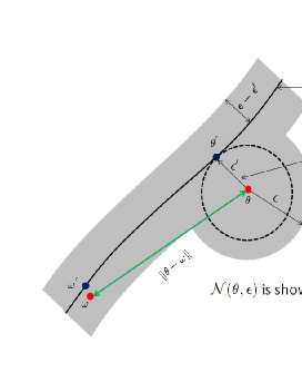
Figure 1: If $\theta$ and $\omega$ are close to two values of parameters $\theta^{\prime}$ and $\omega^{{}^{\prime}}$ with identical probability distribution, then it is be hard to distinguish between them from sampled data, even when $\|\theta-\omega\|$ is large.

The main result in this section is Theorem 2.8, which shows that there exists an algorithm to learn the parameters of a polynomial distribution using a polynomial number of samples.

We start with the outline of the standard parameter learning problem. Let $p_{\mathbb{\theta}}$, ${\mathbb{\theta}}=(\theta^{1},\ldots,\theta^{m}),\theta\in\Theta\subset{\mathbb{R}}^{m}$ be a $m$-parametric family of probability distributions in ${\mathbb{R}}^{l}$. The problem of parameter learning is the following: given precision $\epsilon$ and confidence $\delta$, and some number $n(\epsilon,\delta)$ of points sampled from $p_{\theta}$, we need to provide an estimate $\hat{\theta}$, such that $\|\hat{\theta}-\theta\|<\epsilon$ with probability at least $1-\delta$.

However, for many families identifying the values of parameters uniquely is impossible, due to the fact that several different values of parameters may correspond to the same probability distribution. Moreover, if two values of parameters, say, ${\theta}$ and $\omega$ are close to two values of parameters, $\theta^{\prime}$ and $\omega^{\prime}$ respectively, which have identical probability distributions, then it may be hard to distinguish between them. This situation is illustrated in Fig. 1. These observations suggests that a more general formulation of learning distribution parameters needs to take these into account. A mathematical formalization of the more general of learnability will be given in Eq.1, which defines a notion of a neighborhood taking parameters with identical probability distribution into account. An $\epsilon$-”neighborhood” of ${\theta}$, ${\cal N}({\theta},\epsilon)$, is shown in gray in Fig. 1. We will also introduce the notion of the radius of identifiability ${\mathscr{R}}(\theta)$ (definition 2.9) to give a quantification of how hard it may be to identify the parameters. For example, parameters $\theta$ for which ${\mathscr{R}}(\theta)=0$ cannot be identified given any amount of data. In Fig. 1, the radius of identifiability ${\mathscr{R}}({\theta})$ is equal to $\epsilon^{\prime}$.

For mixtures of Gaussians any permutation of the mixture components has the same distribution, while a component with zero mixing weight may have arbitrary mean/covariance. If two components have the same mean/covariance pair, then the mixing coefficients are not defined uniquely. However, assuming that the mean/variance pairs for any two components are different and that the mixing coefficients are non-zero, the parameters are defined uniquely up to a permutation of components (see Section 2).

Our main Theorem 2.8 applies even when parameters of a probability distributions are not defined uniquly, including the standard definition of parameter learning as a special case (see Corollary 2.10 and Corollary 2.11).

In Subsection 2.1 we prove the basic properties of polynomial families, including the key result, Theorem 2.3, which shows that a finite set of moments uniquely determines the distribution.

In Subsection 2.2 we define the extended notion of a neighborhood ${\cal N}({\theta},\epsilon)$ and discuss its basic properties. We proceed to obtain the main technical result, a lower bound in Theorem 2.5. This, together with the upper bound in Proposition 2.7 allows us to set up a grid search to prove the main Theorem 2.8. We also define the radius of identifiability, and derive Corollary 2.10 and Corollary 2.11.

2.1 Polynomial Families and Finite Sets of Moments

We start by assuming that the parameter set $\Theta$ is a compact semi-algebraic subset of ${\mathbb{R}}^{m}$. Recall that a semi-algebraic set in ${\mathbb{R}}^{m}$ is a finite union of sets defined by a system of algebraic equations and inequalities. A sphere, a polytope, the sets of symmetric and orthogonal matrices are all examples of semi-algebraic sets. For example, a typical family of Gaussian mixture distributions with bounded means and bounded (in norm) covariance matrices would satisfy this condition.

The family of semi-algebraic sets is closed under finite union, intersection and taking complements. Importantly, the Tarski-Seidenberg theorem states that a linear projection of a semi-algebraic set is also semi-algebraic. This is equivalent to the elimination of quantifiers for semi-algebrac sets, which we will need shortly. See [3] for a review of results on real algebraic geometry.

Definition 2.1 (Polynomial family).

We call the family $p_{\theta}$ a polynomial family, if each (raw $l$-dimensional) moment $M_{i_{1},\ldots,i_{l}}(\theta)=\int x_{1}^{i_{1}}\ldots x_{l}^{i_{l}}\,dp_{\theta}$ of the distribution exists and can be represented as a polynomial of the parameters $(\theta^{1},\ldots,\theta^{m})$. We also require that each $p_{\theta}$ should be defined uniquely by its moments.

We will order the moments $M_{i_{1},\ldots,i_{l}}$ lexicographically and denote them by $M_{1}({\theta}),\ldots,M_{n}({\theta}),\ldots$ In the one-dimensional case this corresponds to the standard ordering of the moments.

As it turns out, most of the common families of probability distributions are, in fact, polynomial (see Appendix A). Moreover, a mixture, a product or a linear transformation of polynomial families is also a polynomial family, as stated in the following

Lemma 2.2.

Let $p_{\theta}$, $\theta\in\Theta$ and $q_{\omega}$, $\omega\in\Omega$ be polynomial families. Then the following families are also polynomial:
(a) the family $w_{1}p_{\theta}+w_{2}q_{\omega}$, $w_{1},w_{2}\in{\mathbb{R}}$, $w_{1}+w_{2}=1$.
(b) the family $p_{{\theta},\omega}(x,y)=p_{\theta}(x)\times p_{\omega}(y)$, $({\theta},\omega)\in\Theta\times\Omega$.
(c) the family $p_{A\theta}$, where $A\in{\mathbb{R}}^{m\times m}$ is a fixed matrix and $A\theta\in\Theta\subset{\mathbb{R}}^{m}$.

The proof follows directly from the linearity of the integral, the Fubini’s theorem and the fact that polynomial functions stay polynomial under a linear change.

Note that a multivariate Gaussian distribution is a product of univariate Gaussians along its principal directions of the covariance matrix. Since the standard coordinates can be transformed to principal coordinates by a linear transformation, a multivariate Gaussian is a polynomial family. Hence a general mixture of $k$ multivariate normal distributions in ${\mathbb{R}}^{l}$ is also a polynomial family with $lk+\frac{1}{2}l(l+1)k+k-1$ parameters.

Let us now recall that a family $p_{\theta}$, is called identifiable if $p_{{{\theta_{1}}}}\neq p_{{{\theta_{2}}}}$ for any ${{\theta_{1}}}\neq{{\theta_{2}}}$. We will now prove the following

Theorem 2.3.

Let $p_{\theta}$ be a polynomial family of distributions. Then there exists a positive integer $N$, such that $p_{{\theta_{2}}}=p_{{\theta_{1}}}$ if and only if $M_{i}({{\theta_{1}}})=M_{i}({{\theta_{2}}})$ for all $i=1,\ldots,N$. In the case when the family $p_{\theta}$ is identifiable, the first $N$ moments are sufficient to uniquely identify the parameter $\theta$.

Proof:
Since Let $p_{\theta}$ is a polynomial family, each $M_{i}({\theta})$ is a polynomial of ${\theta}$. Let ${{\theta_{1}}}=({\theta}_{1}^{1},\ldots,{\theta}_{1}^{m})$ and ${{\theta_{2}}}=({\theta}_{2}^{1},\ldots,{\theta}_{2}^{m})$. Let

$$P_{i}({\theta}_{1}^{1},\ldots,{\theta}_{1}^{m},{\theta}_{2}^{1},\ldots,{\theta}_{2}^{m})=M_{i}({{\theta_{1}}})-M_{i}({{\theta_{2}}})$$

be a polynomial of $2m$ variables. Now let ${\cal I}_{j}$ be the ideal in the ring of polynomials of $2m$ variables generated by the polynomials $P_{1},\ldots,P_{j}$. Thus we have an increasing sequence of ideals ${\cal I}_{1}\subset{\cal I}_{2}\subset{\cal I}_{3}\ldots$ Let ${\cal I}=\cup_{j=1}^{\infty}~{}{\cal I}_{j}$. By the Hilbert basis theorem, the ideal $\cal I$ is finitely generated, which implies that for some $N$ large enough, ${\cal I}_{N}$ contains all of the generators. Therefore for any $M\geq N$ we can write

$$P_{M}({{\theta_{1}}},{{\theta_{2}}})=\sum\limits_{i=1}^{N}a_{i}({{\theta_{1}}},{{\theta_{2}}})P_{i}({{\theta_{1}}},{{\theta_{2}}})$$

for some polynomials $a_{i}$. Thus if $P_{i}({{\theta_{1}}},{{\theta_{2}}})=0$ for $i=1,\ldots,N$ then $P_{i}({{\theta_{1}}},{{\theta_{2}}})=0$ for any $i$. Recalling the definition of $P_{M}$, we conclude that all moments of $p_{{\theta_{1}}}$ and $p_{{\theta_{2}}}$ coincide if and only if the first $N$ moments of these distributions are the same. Since the sequence of moments defines the distribution uniquely, the statement of the theorem follows. $\Box$

2.2 Learning Polynomial Families

We will now introduce a notion of an $\epsilon$-”neighbourhood” of a point, which takes into account that different parameters may have identical probability distribution. We proceed to prove the main Theorem 2.8 and a few corollaries, showing that the standard parameter learning problem becomes a special case of the result.

Let ${\cal E}(\theta)=\{\omega|p_{\omega}=p_{\theta}\}$ be the set of parameters $\omega$ which have distributions same as $p_{\theta}$. We note that the distributions corresponding to different values of parameters in the set ${\cal E}(\theta)$ are identical and hence cannot be distinguished from each other given any amount of sampled data. We now define

$${\cal N}(\theta,\epsilon)=\{\omega\in\Theta|\,\exists_{\omega^{\prime},{\theta}^{\prime}\in\Theta,0<\epsilon^{\prime}<\epsilon}~{}\|\omega-\omega^{\prime}\|<\epsilon^{\prime},\omega^{\prime}\in{\cal E}(\theta^{\prime}),\|{\theta}^{\prime}-\theta\|<\epsilon-\epsilon^{\prime}\}$$ (1)

In other words, $\omega$ belongs to ${\cal N}(\theta,\epsilon)$ if it is within $\epsilon^{\prime}<\epsilon$ distance of a parameter value which has the same probability distribution as a parameter value within $\epsilon-\epsilon^{\prime}$ of $\theta$. This definition is illustrated graphically in Fig. 1. We observe the following properties of ${\cal N}(\theta,\epsilon)$:

1. (Symmetry) If ${{\theta_{1}}}\in{\cal N}({{\theta_{2}}},\epsilon)$ then ${{\theta_{2}}}\in{\cal N}({{\theta_{1}}},\epsilon)$.

2. ($\epsilon$-ball) An $\epsilon$-ball $B(\theta,\epsilon)$ around $\theta$ is contained in ${\cal N}(\theta,\epsilon)$. If $B(\theta,\epsilon)$ is an identifiable family, then $B(\theta,\epsilon)={\cal N}(\theta,\epsilon)$.

3. (Equivalence) If $p_{{\theta_{1}}}=p_{{\theta_{2}}}$, then ${{\theta_{1}}}\in{\cal N}({{\theta_{2}}},\epsilon)$ for any $\epsilon>0$.

Thus ${\cal N}(\theta,\epsilon)$ can be viewed as an “$\epsilon$-ball” around $\theta$ taking probability distribution into account. For example, values of parameters with identical probability distributions cannot be distinguished by this metric, which is consistent with statistical identifiability.

Lemma 2.4.

${\cal N}(\theta,\epsilon)$ is an open semi-algebraic set.

Proof:${\cal N}(\theta,\epsilon)$ is open since, a sufficiently small open ball around any point $\omega\in{\cal N}(\theta,\epsilon)$ is also contained in ${\cal N}(\theta,\epsilon)$. To see that it is algebraic we recall that by Theorem 2.3 there exists an $N$, such that ${{\theta_{1}}}\in{\cal E}({{\theta_{2}}})$ if and only if

$$Q({{\theta_{1}}},{{\theta_{2}}})\mathrel{\stackrel{{\scriptstyle\mathop{\rm def}}}{{=}}}\sum_{i=0}^{N}(M_{i}({{\theta_{1}}})-M_{i}({{\theta_{2}}}))^{2}=0$$ (2)

which is an algebraic condition. Hence, by applying the Tarski-Seidenberg theorem to eliminate the existential quantifiers in Eq. 1, we see that ${\cal N}(\theta,\epsilon)$ is semi-algebraic. $\Box$

Theorem 2.5 (Lower bound).

Let $p_{\theta}$ be a polynomial family. There exists $N\in{\mathbb{N}}$ and $t>0$, such that for any sufficiently small $\epsilon>0$ and any ${{\theta_{1}}},{{\theta_{2}}}\in\Theta$, if $|M_{i}({{\theta_{1}}})-M_{i}({{\theta_{2}}})|>\epsilon$ for at least one $i\leq N$, then ${{\theta_{1}}}\notin{\cal N}({{\theta_{2}}},O(\epsilon^{t}))$.

Proof:
Choose $N$ as in Theorem 2.3. We start by observing we can replace the condition

$|M_{i}({{\theta_{1}}})-M_{i}({{\theta_{2}}})|>\epsilon$ by

$$Q({{\theta_{1}}},{{\theta_{2}}})\mathrel{\stackrel{{\scriptstyle\mathop{\rm def}}}{{=}}}\sum_{i=1}^{N}|M_{i}({{\theta_{1}}})-M_{i}({{\theta_{2}}})|^{2}>N{\epsilon^{2}}$$

in the statement of the theorem. Since the existence of $t$ is not affected by the substitution of $N{\epsilon^{2}}$, instead of $\epsilon$, to simplify the matters we will assume that $Q({{\theta_{1}}},{{\theta_{2}}})>\epsilon$.

From Theorem 2.3 we recall that if for some $i\leq N$ $|Q({{\theta_{1}}},{{\theta_{2}}})|\neq 0$ then $p_{{\theta_{1}}}\neq p_{{\theta_{2}}}$. Let $\delta$ be a positive real number. Consider the set $X=\{{{\theta_{1}}},{{\theta_{2}}}|{{\theta_{1}}}\in{\cal N}({{\theta_{2}}},\delta)\}$. From Lemma 2.4 and the fact that the relationship ${{\theta_{1}}}\in{\cal N}({{\theta_{2}}},\delta)$ is symmetric, it follows that $X$ is an open subset of $\Theta\times\Theta$. Hence the set $\Theta\times\Theta-X=\{{{\theta_{1}}},{{\theta_{2}}}\in\Theta,{{\theta_{1}}}\notin{\cal N}({{\theta_{2}}},\delta))\}$ is compact and since $Q({{\theta_{1}}},{{\theta_{2}}})>0$ for any $({{\theta_{1}}},{{\theta_{2}}})\in\Theta\times\Theta-X$ we have

$$\inf_{{{\theta_{1}}},{{\theta_{2}}}\in\Theta,{{\theta_{1}}}\notin{\cal N}({{\theta_{2}}},\delta))}Q({{\theta_{1}}},{{\theta_{2}}})>0$$ (3)

By an argument following that in Lemma 2.4 we see that $X$ and hence its complement are semi-algebraic sets.

Consider now the set $S_{\delta}$, $\delta>0$ given by the following expression

$$S_{\delta}=\{\epsilon>0\,|\,\forall_{{{{\theta_{1}}},{{\theta_{2}}}\in\Theta}}~{}~{}({{\theta_{1}}}\notin{\cal N}({{\theta_{2}}},\delta))\Rightarrow Q(\theta_{1},\theta_{2})>\epsilon\}.$$ (4)

Since these logical statements can be expressed as semi-algebraic conditions, by the Tarski-Seidenberg theorem $S_{\delta}$ is a semi-algebraic subset of ${\mathbb{R}}$. Let $\epsilon(\delta)=\inf S_{\delta}$. From Eq.3 we have that $\epsilon(\delta)>0$ for any positive $\delta$. Since the number $\epsilon(\delta)>0$ is easily written using quantifiers and algebraic conditions, the Tarski-Seidenberg theorem implies that it is a semi-algebraic set and hence satisfies some algebraic equation whose coefficients are polynomial in $\delta$.

We write this polynomial as $q(x)=q_{M}(\delta)x^{M}+\ldots+q_{0}(\delta)$, such that $q(\epsilon(\delta))=0$. We can assume that $q_{0}(\delta)$ is not identically zero (dividing by an appropriate power of $x$ if necessary). From Lemma 2.6 we see that if $q(\epsilon(\delta))=0$ then

$$\epsilon(\delta)>\frac{|q_{0}(\delta)|}{\sum_{i=1}^{M}|q_{i}(\delta)|}.$$

The last quantity is a ratio of two polynomials in $\delta$ and can thus be lower bounded by $C(\delta^{t^{\prime}})$, so that $\epsilon(\delta)>C\delta^{t^{\prime}}$ for some $t^{\prime}>0$, when $\delta$ is sufficiently small.

Putting $t=\frac{1}{t^{\prime}}$ and recalling the definition of $S_{\delta}$, we see that $Q(\theta_{1},\theta_{2})<\epsilon$, implies ${{\theta_{1}}}\in{\cal N}({{\theta_{2}}},O(\epsilon^{t}))$, which completes the proof of the theorem. $\Box$

Lemma 2.6.

Let $\delta$ be a positive root of the polynomial $q(x)=a_{M}x^{M}+\ldots+a_{0}$, $a_{0}\neq 0$. Then $\delta>\min(\frac{\sum_{i=1}^{M}|a_{i}|}{|a_{0}|},1)$.

Proof:We have $\delta(\sum_{i=1}^{M}a_{i}\delta^{i-1})=-a_{0}$. For $0<\delta<1$ we have $\sum_{i=1}^{M}a_{i}\delta^{i-1}<\sum_{i=1}^{M}|a_{i}|$, and the statement follows. $\Box$

Proposition 2.7 (Upper bound).

Let $p_{\theta}$ be a polynomial family. For any $N\in{\mathbb{N}}$ there exists a $C>0$, such that

$$\sum_{i=1}^{N}|M_{i}({{\theta_{1}}})-M_{i}({{\theta_{2}}})|^{2}<C\|{{\theta_{1}}}-{{\theta_{2}}}\|^{2}.$$

If $\Theta$ is contained in a ball of diameter $B$, then $C$ is bounded from above by a polynomial of $B$.

Proof:To prove the claim it is sufficient to show that each summand $|M_{i}({{\theta_{1}}})-M_{i}({{\theta_{2}}})|^{2}$ is bounded from above by $C^{\prime}\|{{\theta_{1}}}-{{\theta_{2}}}\|^{2}$, which is equivalent to proving that $\frac{|M_{i}({{\theta_{1}}})-M_{i}({{\theta_{2}}})|}{\|{{\theta_{1}}}-{{\theta_{2}}}\|}<\sqrt{C^{\prime}}$. We now observe that by the mean value theorem

$$\frac{|M_{i}({{\theta_{1}}})-M_{i}({{\theta_{2}}})|}{\|{{\theta_{1}}}-{{\theta_{2}}}\|}\leq\sup_{\theta\in\Theta}\|{\mathop{\rm grad}}(M_{i})({\theta})\|$$

where ${\mathop{\rm grad}}$ is the gradient of the function $M_{i}$. Since $M_{i}$ is a polynomial, all elements of the vector ${\mathop{\rm grad}}(M_{i})$ are polynomial in $\theta$. Therefore

$$\sup_{\theta\in\Theta}\|{\mathop{\rm grad}}(M_{i})({\theta})\|<C^{\prime\prime}B^{t}$$

where $t$ is the maximum degree of these polynomials and $C^{\prime\prime}$ is an appropriate constant. This implies the statement of the Proposition. $\Box$

Now we have the following:

Theorem 2.8.

There exists an algorithm, which, given $\epsilon>0$ and $1>\delta>0$, and $P(\frac{1}{\epsilon},\frac{1}{\delta},B)$ samples from $p_{\theta},\theta\in\Theta$, where $\Theta$ is the set of parameters within a ball of radius $B$ and $P$ is a polynomial depending only on the distribution family, outputs $\hat{\theta}$, s.t. $\hat{\theta}\in{\cal N}(\theta,\epsilon)$ with probability at least $1-\delta$. The algorithm also requires a polynomial number of operations.

Proof:From Theorem 2.5 it follows that there exists an $N\in{\mathbb{N}}$ and $t>0$, such that if $\forall_{i=1,\ldots,N}|M_{i}({{\hat{\theta}}})-M_{i}({\theta})|<\epsilon^{t}$, than ${{\hat{\theta}}}\in{\cal N}({\theta},\epsilon)$. Thus it is sufficient to estimate each moment within $O(\epsilon^{t})$. From Lemma D.1 (moment estimation) this can be done with probability $1-\delta$ given a number of sample points $\operatorname*{poly}(\frac{1}{\epsilon^{t}},\frac{1}{\delta})=\operatorname*{poly}(\frac{1}{\epsilon},\frac{1}{\delta})$ by computing the empirical moments of the sample. Once we have precise estimates of the first moments a simple grid search suffices to find the corresponding values of parameters. Indeed, suppose that $\Theta$ is contained in a ball of radius $B$ in ${\mathbb{R}}^{m}$. Then the desired estimate can be obtained by conducting a grid search over a rectangular grid of size $O(\frac{\epsilon^{t}}{N\sqrt{m}})$ and invoking Proposition 2.7. We see that the number of operations is polynomial in $\epsilon$ and the main theorem is proved. $\Box$

To simplify further discussion we will now define the radius of identifiability:

Definition 2.9.

As before let $p_{\theta}$, $\theta\in\Theta$ be a family of probability distributions. For each $\theta$ we define the radius of identifiability as follows

$${\mathscr{R}}(\theta)=\sup\{r>0|\forall{{\theta_{1}}}\neq{{\theta_{2}}},(\|{{\theta_{1}}}-\theta\|<r,\|{{\theta_{2}}}-\theta\|<r)\Rightarrow(p_{{\theta_{1}}}\neq p_{{\theta_{2}}})\}$$

In other words, ${\mathscr{R}}(\theta)$ is the largest number, such that the open ball of radius ${\mathscr{R}}(\theta)$ around $\theta$ intersected with $\Theta$ is an identifiable (sub)family of probability distributions. If no such ball exists, ${\mathscr{R}}(\theta)=0$.

From Theorem 2.8 and the definition of the radius of identifiability we have the following

Corollary 2.10.

There exists an algorithm, such that, given $\epsilon>0$, for any identifiable $\theta\in\Theta$, where $\Theta$ is the set of parameters within a ball of radius $B$, it outputs ${{\hat{\theta}}}$ within $\min(\epsilon,{\mathscr{R}}(\theta))$ of ${\theta}$ with probability $1-\delta$, using a number of sample points from $p_{\theta}$ polynomial in $\max\left(\frac{1}{\epsilon},\frac{1}{{\mathscr{R}}(\theta)}\right)$, $\frac{1}{\delta}$ and $B$.

Corollary 2.11.

More generally, if $\theta\in\Theta$, where $\Theta$ is the set of parameters within a ball of radius $B$, is not identifiable but, ${\cal E}(\theta)=\{{\theta}_{1},\ldots,{\theta}_{k}\}$ is a finite set, there exists an algorithm, such that, given $\epsilon>0$, it outputs ${{\hat{\theta}}}$ within $\min(\epsilon,\min_{j}{\mathscr{R}}(\theta_{j}))$ of ${\theta}_{i}$ for some $i\in\{1,\ldots,k\}$ with probability $1-\delta$, using a number of sample points from $p_{\theta}$ polynomial in $\max\left(\frac{1}{\epsilon},\frac{1}{\min_{j}{\mathscr{R}}(\theta_{j})}\right)$ and $\frac{1}{\delta}$.

This last result is what we need to analyze Gaussian mixture model in the next Section.

Remark: It is important to note that the radius of identifiability depends on the choice of family $\Theta$. Specifically, the radius is a decreasing function on the family of the sets $\Theta$ ordered by inclusion.

3 Gaussian Distributions and Polynomially Reducible High Dimensional Families

The main result of this section is to show that there exists an algorithm for estimating parameters of high-dimensional Gaussian mixture distributions in time polynomial in the dimension $n$ and other parameters. We note that the techniques from the previous section cannot be applied directly to high-dimensional distributions since the number of parameters generally increases with dimension. Instead our approach will be to show that parameters of high-dimensional Gaussians can be estimated using $\operatorname*{poly}(n)$ linear projections to linear subspaces, whose dimension is independent of $n$. We will call this property polynomial reducibility and will also briefly discuss some other families satisfying this condition later in the section.

We will now specifically discuss the case of a mixture of Gaussian distributions. Let $p_{\theta}=\sum_{i=1}^{k}w_{i}N(\mu_{i},\Sigma_{i})$ be a mixture of $k$ Gaussian distributions in ${\mathbb{R}}^{n}$, with means $\mu_{i}$ and covariance matrices $\Sigma_{i}$. Let us consider the parameters of the distribution $\theta=(\mu_{1},\Sigma_{1},w_{1},\ldots,\mu_{k},\Sigma_{k},w_{k})$ as a single vector (thus flattening the covariance matrices). We take the usual Euclidean distance in this space (which, in fact, corresponds to the Frobenius distance for the covariance matrices).

We will assume that the number of components $k$ is fixed. We note that any permutation of the mixture components leads to the same density function and hence cannot be identified from data. On the other hand, it is well known ([22]) that the density of the distribution determines the parameters uniquely up to a permutation, if and only if any two components with the same means have different covariance matrices and no mixing coefficient is equal to zero.

The main result of the section is given by the following

Theorem 3.1.

Let $p_{\theta}=\sum_{i=1}^{k}w_{i}N(\mu_{i},\Sigma_{i}),\theta\in\Theta$, where $\Theta$ is the set of parameters within a ball of radius $B$, be a mixture of Gaussian distributions in ${\mathbb{R}}^{n}$ with radius of identifiability ${\mathscr{R}}(\theta)$. Then there exists an algorithm , which, given $\epsilon>0$ and $1>\delta>0$, and $poly\left(n,\max\left(\frac{1}{\epsilon},\frac{1}{{\mathscr{R}}(\theta)}\right),\frac{1}{\delta},B\right)$ samples from $p_{\theta}$, with probability greater than $(1-\delta)$, outputs a parameter vector $\hat{\theta}=\left((\hat{\mu}_{1},\hat{\Sigma}_{1},\hat{w}_{1}),\ldots,(\hat{\mu}_{k},\hat{\Sigma}_{k},\hat{w}_{k})\right)\in\Theta$, such that there exists a permutation $\sigma:\{1,2,\ldots,k\}\rightarrow\{1,2,\ldots,k\}$ satisfying,

$$\sum_{i=1}^{k}\left(\|\mu_{i}-\hat{\mu}_{\sigma(i)}\|^{2}+\|\Sigma_{i}-\hat{\Sigma}_{\sigma(i)}\|^{2}+|w_{i}-\hat{w}_{\sigma(i)}|^{2}\right)\leq\epsilon^{2}$$

We note that the radius of identifiability ${\mathscr{R}}(\theta)$ can be calculated explicitly from the Proposition 3.3:

$$({\mathscr{R}}(\theta))^{2}=\min\left(\frac{1}{4}\min_{i\neq j}\left(\|\mu_{i}-\mu_{j}\|^{2}+\|\Sigma_{i}-\Sigma_{j}\|^{2}\right),\min_{i}w_{i}^{2}\right)$$

Thus if the mean/variance pairs for any two components are different with difference bounded from below and the minimum mixing weight is is also bounded from below, then we have explicit lower bound for ${\mathscr{R}}(\theta)$.

In fact even when ${\mathscr{R}}(\theta)$ is not known in advance, it can be estimated from data as:

Theorem 3.2.

Let $p_{\theta}=\sum_{i=1}^{k}w_{i}N(\mu_{i},\Sigma_{i}),\theta\in\Theta$, where $\Theta$ is the set of parameters within in a ball of radius $B$, be a mixture of Gaussian distributions in ${\mathbb{R}}^{n}$ with radius of identifiability ${\mathscr{R}}(\theta)$. Then there exists an algorithm , which, given $\epsilon>0$ and $1>\delta>0$, and $poly\left(n,\frac{1}{\epsilon},\frac{1}{\delta},B\right)$ samples from $p_{\theta}$ outputs whether ${\mathscr{R}}(\theta)<\epsilon$ with probability greater than $1-\delta$.

$\Box$

The rest of the section is structured as follows:

In subsection 3.1 we discuss various properties of Gaussian mixture distributions. In particular we derive the formula for the radius of identifiability (Proposition 3.3) and show that there exists a low-dimensional projection such that the radius of identifiability changes by at most a linear factor (Theorem 3.7).

In subsection 3.2 we give a sketch for the proof of the main theorem, showing how the parameters of a high-dimensional distribution can be estimated from a polynomial number of projections. The details of the proof as well as the proof of Theorem 3.2 are given in the appendix C.

Finally, we note that our results apply to high-dimensional distributions which are not mixtures of Gaussians with a fixed number of components. For example, a product of $n$ $1$-dimensional Gaussian mixture distributions, which is a Gaussian mixture distribution in $n$ dimensions with $k^{n}$ components, can be easily learned using our methods. The same applies to other product distributions whose components are polynomial families.

3.1 Gaussian Distributions

Proposition 3.3.

Let $p_{\theta}=\sum_{i=1}^{k}w_{i}N(\mu_{i},\Sigma_{i})$, $\theta\in\Theta$ be a family of mixtures of Gaussian distributions in ${\mathbb{R}}^{n}$ with non-zero mixing weights. Then the following inequality is satisfied:

$$({\mathscr{R}}(\theta))^{2}\geq\min\left(\frac{1}{4}\min_{i\neq j}\left(\|\mu_{i}-\mu_{j}\|^{2}+\|\Sigma_{i}-\Sigma_{j}\|^{2}\right),\min_{i}w_{i}^{2}\right).$$ (5)

Moreover, suppose $\Theta$ is a convex set such that it contains all possible mixing coefficients $(w_{1},\ldots,w_{k})$ for any fixed set of means and variances

In this case the inequality becomes an equality:

$$({\mathscr{R}}(\theta))^{2}=\min\left(\frac{1}{4}\min_{i\neq j}\left(\|\mu_{i}-\mu_{j}\|^{2}+\|\Sigma_{i}-\Sigma_{j}\|^{2}\right),\min_{i}w_{i}^{2}\right)$$ (6)

In particular, the radius of identifiability is invariant under the permutation of components.

Proof:We will start by proving the inequality 5. Suppose that the distributions $p_{\theta^{\prime}}$ and $p_{\theta^{\prime\prime}}$ have the same density. To prove the inequality, we need to show that at least one of ${\theta}^{\prime}$, ${\theta}^{\prime\prime}$ is no closer to ${\theta}$ then the right hand side of the inequality 5.

Let us first consider the case when there is no pair $i\neq j$, s.t. $\mu^{\prime}_{i}=\mu^{{}^{\prime\prime}}_{j}$ and $\Sigma_{i}^{\prime}=\Sigma^{{}^{\prime\prime}}_{j}$. In that case that case at least one of the mixing coefficients for one of the mixtures must be equal to zero. That implies that either $\|{\theta}-{\theta}^{\prime}\|\geq\min_{i}w_{i}$ or $\|{\theta}-{\theta}^{\prime\prime}\|\geq\min_{i}w_{i}$, which is consistent with the 5.

Alternatively, suppose that for some $i\neq j$ we have $(\mu_{i}^{\prime},\Sigma_{i}^{\prime})=(\mu_{j}^{\prime\prime},\Sigma_{j}^{\prime\prime})$. Put $v^{\prime}=(\mu_{i}^{\prime},\Sigma_{i}^{\prime})=(\mu_{j}^{\prime\prime},\Sigma_{j}^{\prime\prime})$, $v_{1}=(\mu_{i},\Sigma_{i})$, $v_{2}=(\mu_{j},\Sigma_{j})$. We see that

$$\|\theta^{\prime\prime}-\theta\|^{2}+\|\theta^{\prime}-\theta\|^{2}\geq\|v^{\prime}-v_{1}\|^{2}+\|v^{\prime}-v_{2}\|^{2}\geq\frac{1}{2}\|v_{1}-v_{2}\|^{2}=$$

$$=\frac{1}{2}\|\mu_{i}-\mu_{j}\|^{2}+\frac{1}{2}\|\Sigma_{i}-\Sigma_{j}\|^{2}$$

Therefore, $\max\{\|\theta^{\prime}-\theta\|^{2},\|\theta^{\prime\prime}-\theta\|^{2}\}\geq\frac{1}{4}(\|\mu_{i}-\mu_{j}\|^{2}+\|\Sigma_{i}-\Sigma_{j}\|^{2})$ which is again consistent with Inequality 5 and together with the first case implies the inequality.

To show Eq. 6 we need to observe that the bound is tight. Again we consider two possible cases. If the minimum in the right hand side of Eq. 6 is equal to the square of one of the mixing weights, say, $w_{i}$, construct ${\theta}^{\prime}$ by putting $w_{i}^{\prime}=0$ and keeping the rest of the parameters of $\theta$. We see that $\|{\theta}^{\prime}-{\theta}\|=w_{i}$. By slightly perturbing $\mu^{\prime}$, we see that there exists a ${\theta}^{\prime\prime}$ arbitrarily close (but not equal)to ${\theta}^{\prime}$ with the same probability density. Thus the radius of identifiability cannot exceed $w_{i}$.

Alternatively the minimum in the right hand side of Eq. 6 could be equal to $\frac{1}{4}\left(\|\mu_{i}-\mu_{j}\|^{2}+\|\Sigma_{i}-\Sigma_{j}\|^{2}\right)$ for some $i\neq j$. Construct ${\theta}^{\prime}$ by putting $\mu^{\prime}_{i}=\mu^{\prime}_{j}=\frac{1}{2}(\mu_{i}-\mu_{j})$ and $\Sigma^{\prime}_{i}=\Sigma^{\prime}_{j}=\frac{1}{2}(\Sigma_{i}-\Sigma_{j})$ and keeping the rest of the parameters of ${\theta}$. It is easy to see that $\|{\theta}^{\prime}-{\theta}\|^{2}=\frac{1}{4}\left(\|\mu_{i}-\mu_{j}\|^{2}+\|\Sigma_{i}-\Sigma_{j}\|^{2}\right)$. Note that $\theta^{\prime}\in\Theta$ by the convexity condition. By perturbing $w_{i}$ and $w_{j}$ slightly, and keeping the rest of parameters fixed, we can obtain ${\theta}^{\prime\prime}$ arbitrarily close to ${\theta}^{\prime}$ with the same probability density. Hence the radius of identifiability does not exceed $\frac{1}{4}\left(\|\mu_{i}-\mu_{j}\|^{2}+\|\Sigma_{i}-\Sigma_{j}\|^{2}\right)$, which completes the proof. $\Box$

From the discussion above we have the following

Corollary 3.4.

Let $\Theta$ be a convex set, such that for any $\theta\in\Theta$ all mixing coefficients $w_{i}$ are nonzero. Then

$$({\mathscr{R}}(\theta))^{2}=\frac{1}{4}\min_{i\neq j}\left(\|\mu_{i}-\mu_{j}\|^{2}+\|\Sigma_{i}-\Sigma_{j}\|^{2}\right)$$ (7)

It is also easy to see that the radius of identifiability satisfies a type of triangle inequality and that under any permutation of (mean, covariance matrix, mixing weight) triples the radius of identifiability does not change. This is expressed in the following two lemmas (the straightforward proofs are omitted):

Lemma 3.5.

Let $p_{\theta}=\sum_{i=1}^{k}w_{i}N(\mu_{i},\Sigma_{i})$, $\theta\in\Theta$ be a family of mixtures of Gaussian distributions in ${\mathbb{R}}^{n}$. For any $\theta_{1},\theta_{2}\in\Theta$ such that $\theta_{1}\in\mathcal{N}(\theta_{2},\epsilon)$ for some $\epsilon>0,|{\mathscr{R}}(\theta_{1})-{\mathscr{R}}(\theta_{2})|\leq\epsilon$.

Lemma 3.6.

Let $p_{\theta}=\sum_{i=1}^{k}w_{i}N(\mu_{i},\Sigma_{i}),\theta\in\Theta$ be a mixture of Gaussian distributions in ${\mathbb{R}}^{n}$. Suppose $\theta$ is represented as $\theta=(\theta_{1},\theta_{2},\ldots,\theta_{k})$, where $\theta_{i}=(\mu_{i},\Sigma_{i},w_{i})$ is the mean, covariance matrix, mixing weight triple. Let $\theta^{{}^{\prime}}=(\theta_{\sigma(1)},\theta_{\sigma(2)},\ldots,\theta_{\sigma(2)})$, where $\sigma:\{1,2,\ldots,k\}\rightarrow\{1,2,\ldots,k\}$ is a permutation. Then ${\mathscr{R}}(\theta)={\mathscr{R}}(\theta^{{}^{\prime}})$.

From now on, we will assume that $\Theta$ is a sufficiently large ball or cube (with the necessary conditions to make $p_{\theta}$ a valid probability distribution), so that we do not have to worry about convexity and other technical properties.

We now recall that a projection of a Gaussian mixture distribution onto a subspace is a lower-dimensional Gaussian mixture distribution. Specifically, if $p_{\theta}=\sum_{i=1}^{k}w_{i}N(\mu_{i},\Sigma_{i})$, the Gaussian mixture distributions in ${\mathbb{R}}^{n}$, is projected onto a subspace $S$ then the projection is a lower-dimensional Gaussian mixture distribution family $\pi_{S}(p_{\theta})$, parameterized by $P_{S}(\theta)$. In particular, if $S$ is a coordinate plane then $P_{S}$ is a projection operator, which is an identity mapping for the mixing weights, an orthogonal projection onto $S$ for the means and the restriction operator for the covariance matrices of the components, where each covariance matrix is projected to its minor corresponding to the coordinates in $S$.

We will now state the following Theorem whose proof can be found in appendix C.

Theorem 3.7.

Let $p_{\theta}=\sum_{i=1}^{k}w_{i}N(\mu_{i},\Sigma_{i})$, $\theta\in\Theta$ be a Gaussian mixture distribution in ${\mathbb{R}}^{n}$ with radius of identifiability ${\mathscr{R}}(\theta)$. Then there exists a $2k^{2}$-dimensional coordinate plane $S$, such that ${\mathscr{R}}(P_{S}(\theta))\geq\frac{1}{n}{\mathscr{R}}(\theta)$.

3.2 Sketch of the Proof of Theorem 3.1

We present a brief overview of the proof. The technical details can be found in Appendix C. The main idea is to show that parameters of high-dimensional Gaussian mixture can be estimated arbitrarily well using $\operatorname*{poly}(n)$ projections to coordinate subspaces, whose dimension only depends on $k$. Since the dimension of these lower dimensional subspaces is independent of $n$, results from Section 2 can be used to estimate the parameters.

Let $\theta=(\theta_{1},\theta_{2},\ldots,\theta_{k})$, where $\theta_{i}=(\mu_{i},\Sigma_{i},w_{i})$, be the parameter vector after flattening the covariance matrices. Recall that projection of $p_{\theta}$ onto a $2k^{2}$-coordinate plane $T$, will result in a mixture $\pi_{T}(p_{\theta})$, parameterized (with a slight abuse of notation) by $P_{T}(\theta)=(P_{T}(\theta_{1}),P_{T}(\theta_{2}),\ldots,P_{T}(\theta_{k}))$.

Step 1: Let ${\mathscr{R}}(\theta)$ be the radius of identifiability. Theorem 3.7 guarantees the existence of a $2k^{2}$-dimensional coordinate subspace $S$, such that radius of identifiability decreases by at most $\frac{1}{n}$, ${\mathscr{R}}(P_{S}(\theta))\geq\frac{1}{n}{\mathscr{R}}(\theta)$.

To identify such a subspace, we take all $n\choose 2k^{2}$ coordinate projections. For each projection to a subspace $T$ we estimate the parameters using the Theorem 2.8. It is important to note that given $\epsilon^{\prime}$ as input, Theorem 2.8 is guaranteed to produce a value of parameter $\widehat{P_{T}(\theta)}$, such that $|{\mathscr{R}}(\widehat{P_{T}(\theta)})-{\mathscr{R}}(P_{T}({\theta}))|<\epsilon^{\prime}$ (Lemma 3.5) using a number of samples polynomial in $k$ and $\frac{1}{\epsilon^{\prime}}$. Applying the union bound for all $n\choose 2k^{2}$ projections provides an estimate for the radius of identifiability for each projection within $\epsilon^{\prime}$. Choosing $\epsilon^{\prime}$ appropriately (say, $\frac{{\mathscr{R}}({\theta})}{2n}$), and choosing the projection with the largest estimated radius of identifiability, yields a coordinate subspace $S$ with a lower bounded ${\mathscr{R}}(P_{S}({\theta}))$.

The coordinates within $S$ are represented by the horizontally shaded region in Figure 2. We use this space as a starting point for Step 2.

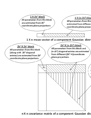
Figure 2: Estimation of high-dimensional Gaussian mixture parameters from $\operatorname*{poly}(n)$ lower-dimensional projections.

Step 2: By applying Corollary 2.11 to the projection $P_{S}({\theta})$, we can estimate the mixing weights, projections of the original means and $2k^{2}\times 2k^{2}$ minors of the covariance matrices corresponding to the coordinates within $S$. We now need to estimate the rest of the parameters using a sample size polynomial on $n$. We do this by estimating each additional coordinate separately. That is for each coordinate $i$ not in $S$ we take $S_{i}=span(S,e_{i})$, where $e_{i}$ is the corresponding coordinate vector. It can be seen that the radius of identifiability does not decrease going from $S$ to $S_{i}$. We show that the $i$’th coordinate of each component mean can be estimated by applying Corollary 2.11 to the projection to $S_{i}$. We repeat this procedure for each of the $n-2k^{2}$ coordinates not in $S$.

To estimate the covariance matrices we proceed similarly, except that we need to estimate entries corresponding to pairs of coordinates $(i,j)$. Now we have two possibilities, since either one of $i,j$ or both of them may not be in $S$. If exactly one of them, say $i$, is not in $S$, projection to $S_{i}$ defined above can be used to estimate the corresponding entry of each covariance matrix. If both $i,j$ are not in $S$, we take the projection onto $S_{ij}=span(S,e_{i},e_{j})$. By applying Corollary 2.11, we show that the $ij$’th entry of covariance matrices can also be estimated.

Thus, after obtaining the initial space $S$, the complete set of parameters can be estimated using at most $n-2k^{2}+{{n-2k^{2}}\choose 2}$ parameter estimations for $2k^{2}+1$ or $2k^{2}+2$-dimensional subspaces.

This procedure is graphically shown in in Figure 2.

4 Conclusion and Discussion

The results of this paper resolve the general problem of polynomial learning of Gaussian mixture distributions. Our results do not require any separation assumptions and apply as long as the mixture is identifiable. For example, they apply even if all components of the mixture have the same mean distribution, as long as the covariance matrices are different and the mixing coefficients are non-zero.

The proof brings the techniques of algebraic geometry to the classical method of moments, an approach that, as far as we know, is new to this domain. We also provide quite general results applicable to learning various low-dimensional families and some observations on high-dimensional families going beyond Gaussian mixture distributions with a fixed number of components. For example, one can also learn products of arbitrary probability distributions in a fixed low-dimensional polynomial family, e.g., a product of $n$ number of $d$-dimensional Gaussians mixtures with $k$ components each (which is a $nd$-dimensional Gaussian mixture distribution with $k^{n}$ components).

We are planning to investigate other applications in learning of the framework presented in this paper. We also note that the methods proposed in the paper can be turned into implementable (and potentially practical) algorithms through the use of tools from computational algebraic geometry. This is also a direction of future investigation.

Appendix

Appendix A Some Polynomial Families of Distributions

In this appendix we provide a partial list comprising the expressions of moments of various univariate probability distributions which form polynomial families. It turns out that most of the commonly used distributions form polynomial families as shown Table 2. In the fifth column of Table 2, we provide either expression for the $i^{th}$ moment or a recurrence relation, which shows that the moments are polynomial in the distribution parameters, along with explicit expressions for the first three moments. These moment expressions and recurrence relations are well known and can be found in, e.g., [15, 21]. In a couple of cases we need a slightly different parameterization, instead of the standard one, to ensure that the moments are polynomial in these new parameters. For example, in standard parametrization, Negative Binomial distribution $NB(r,p)$ is expressed by probability mass function ${x+r-1\choose r-1}(1-p)^{r}p^{x}$. However, if we replace $p$ by a new parameter $m=\frac{p}{1-p}$, then the moments are polynomial in $r$ and $m$. Recurrence relation for this new parameterization can be obtained following the same steps as in [21]. Table 3 we list two families which are not polynomial.

Distribution	$\theta$	Pdf/Pmf $f(x;\theta)$	Mgf $M(t)$	Moments Expression
Gaussian	$\mu,\sigma$	$\frac{1}{\sqrt{2\pi}\sigma}e^{-\frac{(x-\mu)^{2}}{2\sigma^{2}}}$	$e^{\mu t+\frac{\sigma^{2}t^{2}}{2}}$	$\mathbb{E}(X^{i})=\mu\mathbb{E}(X^{i-1})+(i-1)\sigma^{2}\mathbb{E}(X^{i-2})$
				$\mathbb{E}(X)~{}=\mu$
				$\mathbb{E}(X^{2})=\mu^{2}+\sigma^{2}$
				$\mathbb{E}(X^{3})=\mu^{3}+3\mu\sigma^{2}$
Uniform	$a,b$	$\frac{1}{b-a}\mbox{, $a\leq x\leq b$}$	$\frac{e^{tb}-e^{ta}}{t(b-a)}$	$\mathbb{E}(X^{i})=\frac{1}{i+1}\sum_{j=1}^{i}a^{j}b^{i-j}$
				$\mathbb{E}(X)~{}=\frac{a+b}{2}$
				$\mathbb{E}(X^{2})=\frac{a^{2}+ab+b^{2}}{3}$
				$\mathbb{E}(X^{3})=\frac{a^{3}+a^{b}+ab^{2}+b^{3}}{4}$
Gamma	$\beta,m$	$\frac{x^{m-1}e^{-x/\beta}}{\beta^{m}\Gamma(m)}\mbox{, $x>0$}$	$(1-\beta t)^{-m}$	$\mathbb{E}(X^{i})=\prod_{j=0}^{i-1}(m+j)\beta^{i}$
				$\mathbb{E}(X)~{}=m\beta$
				$\mathbb{E}(X^{2})=m(m+1)\beta^{2}$
				$\mathbb{E}(X^{3})=m(m+1)(m+2)\beta^{3}$
Laplace	$\mu,b$	$\frac{1}{2b}e^{-\frac{|x-\mu|}{b}}$	$\frac{e^{\mu t}}{1-b^{2}t^{2}}$	$\mathbb{E}(X^{i})=\sum_{j=0}^{i}\frac{i!b^{j}\mu^{i-j}}{(i-j)!}1_{\{j\mbox{ is even}\}}$
				$\mathbb{E}(X)~{}=\mu$
				$\mathbb{E}(X^{2})=\mu^{2}+2b^{2}$
				$\mathbb{E}(X^{3})=\mu^{3}+6\mu b^{2}$
Exponential	$\lambda$	$\frac{1}{\lambda}e^{-\frac{x}{\lambda}}\mbox{, $x>0$}$	$(1-\lambda t)^{-1}$	$\mathbb{E}(X^{i})=i!\lambda^{i}$
				$\mathbb{E}(X)~{}=\lambda$
				$\mathbb{E}(X^{2})=2\lambda^{2}$
				$\mathbb{E}(X^{3})=6\lambda^{3}$
Chi-Square	$k$	$\frac{x^{\frac{k}{2}-1}e^{-\frac{x}{2}}}{2^{k/2}\Gamma(k/2)}\mbox{, $x>0$}$	$(1-2t)^{-\frac{k}{2}}$	$\mathbb{E}(X^{i})=k(k+2)\cdots(k+2i-2)$
				$\mathbb{E}(X)~{}=k$
				$\mathbb{E}(X^{2})=k(k+2)$
				$\mathbb{E}(X^{3})=k(k+2)(k+4)$
	$\mu,\lambda$	$\sqrt{\frac{1}{2\pi\lambda x^{3}}}e^{-\frac{(x-\mu)^{2}}{2\lambda\mu^{2}x}}$	$e^{\frac{(1-\sqrt{1-2\lambda\mu^{2}t})}{\lambda\mu}}$	$\mathbb{E}(X^{i})=(2i-3)\lambda\mu^{2}\mathbb{E}(X^{i-1})+\mu^{2}\mathbb{E}(X^{i-2})$
Inverse				$\mathbb{E}(X)~{}=\mu$
Gaussian				$\mathbb{E}(X^{2})=\lambda\mu^{3}$
				$\mathbb{E}(X^{3})=3\lambda^{2}\mu^{5}$
Poisson	$\lambda$	$\frac{\lambda^{x}e^{-\lambda}}{x!}$	$e^{\lambda(e^{t}-1)}$	$\mathbb{E}(X^{i})=\lambda\mathbb{E}(X^{i-1})+\lambda\frac{d(\mathbb{E}(X^{i-1}))}{d\lambda}$
				$\mathbb{E}(X)~{}=\lambda$
				$\mathbb{E}(X^{2})=\lambda^{2}+\lambda$
				$\mathbb{E}(X^{3})=\lambda^{3}+3\lambda^{2}+\lambda$
Binomial	$n,p$	${n\choose x}p^{x}(1-p)^{n-x}$	$(1-p+pe^{t})^{n}$	$\mathbb{E}(X^{i})=np\mathbb{E}(X^{i-1})+p(1-p)\frac{d(\mathbb{E}(X^{i-1}))}{dp}$
				$\mathbb{E}(X)~{}=np$
				$\mathbb{E}(X^{2})=n(n-1)p^{2}+np$
				$\mathbb{E}(X^{3})=(n^{3}-3n^{2}+2n)p^{3}+3n(n-1)p^{2}+np$
Geometric	$p$	$(1-\frac{1}{p})^{x}(\frac{1}{p})$	$\frac{1}{p-(p-1)e^{t}}$	$\mathbb{E}(X^{i})=\sum_{j=0}^{\infty}\frac{1}{p}\left(1-\frac{1}{p}\right)^{j}j^{i}$
				$\mathbb{E}(X)~{}=(p-1)$
				$\mathbb{E}(X^{2})=(p-1)(2p-1)$
				$\mathbb{E}(X^{3})=(p-1)(6p^{2}-6p+1)$
	$r,m$	${x+r-1\choose r-1}\frac{m^{x}}{(m+1)^{r+x}}$	$\left(\frac{1}{m+1-me^{t}}\right)^{r}$	$\mathbb{E}(X^{i})=rm\mathbb{E}(X^{i-1})+m(m+1)\frac{d(\mathbb{E}(X^{i-1}))}{dm}$
Negative				$\mathbb{E}(X)~{}=rm$
Binomial				$\mathbb{E}(X^{2})=r(r+1)m^{2}+rm$
				$\mathbb{E}(X^{3})=(r^{3}+3r^{2}+2r)m^{3}+3r(r+1)m^{2}+rm$

Table 2: Common polynomial families and their moments

Distribution	$\theta$	Pdf/Pmf $f(x;\theta)$	Mgf $M(t)$	Moments Expression
Weibull	$k,\lambda$	$\frac{k}{\lambda}\left(\frac{x}{\lambda}\right)^{k-1}e^{-\left(\frac{x}{\lambda}\right)^{k}}$	$\sum_{n-0}^{\infty}\frac{t^{n}\lambda^{n}}{n!}\Gamma\left(1+\frac{n}{k}\right)$	$\mathbb{E}(X^{i})=\lambda^{i}\Gamma\left(1+\frac{i}{k}\right)$
Cauchy	$\lambda,\gamma$	$\frac{1}{\pi\gamma\left[1+\left(\frac{x-\lambda}{\gamma}\right)^{2}\right]}$	Does not exist	Does not exist

Table 3: Examples of some probability distributions that do not belong to polynomial family

Appendix B Separation Preserving Coordinate Planes

Let $p_{\theta}=\sum_{i=1}^{k}w_{i}N(\mu_{i},\Sigma_{i})$ be a mixture of $k$ Gaussian distributions in ${\mathbb{R}}^{l}$, with means $\mu_{i}$ and covariance matrices $\Sigma_{i}$. When this distribution is projected onto any lower dimensional coordinate plane $S$, the corresponding Gaussian mixture $\pi_{S}(p_{\theta})$, parameterized by $P_{S}(\theta)$, has means and covariance matrices represented by $P_{S}(\mu_{i})$ and $P_{S}(\Sigma_{i})$ respectively. We first show that if any pair of means or pair of covariance matrices of the original component Gaussian distributions are separated, then they remain so after projecting the mixture distribution onto some suitable lower dimensional coordinate plane.

Existence of a Coordinate Plane where Projected Means Remain Separated :

Lemma B.1.

For any $\mu_{1},\mu_{2},...,\mu_{k}\in\mathbb{R}^{l}$, there exists a $k^{2}$-coordinate plane $S$ such that,

$$\forall_{i,j},\|P_{S}(\mu_{i})-P_{S}(\mu_{j})\|\geq\|\mu_{i}-\mu_{j}\|\frac{1}{\sqrt{l}}$$

.

Proof:We will use $\mathcal{M}$ to denote a set of indices of coordinate directions of ${\mathbb{R}}^{l}$ and let $S_{\mathcal{M}}$ be the $|\mathcal{M}|$-coordinate plane, where $|\mathcal{M}|$ is the cardinality of $\mathcal{M}$, spanned by the coordinate directions whose indices are in $\mathcal{M}$. Initially $\mathcal{M}$ is empty. Let $\mathcal{A}_{i}=\left\{1,2,\ldots,i-1,i+1,\ldots,k\right\}$. Now consider the pair consisting of $\mu_{1}$ and any other $\mu_{j}$ such that $j\in\mathcal{A}_{1}$. There exists at least one coordinate direction, whose index is say $m$, such that $|\mu_{1,m}-\mu_{j,m}|\geq\|\mu_{1}-\mu_{j}\|\frac{1}{\sqrt{l}}$. Adding $m$ to $\mathcal{M}$, and projecting onto $S_{\mathcal{M}}$, guarantees that $\|P_{S_{\mathcal{M}}}(\mu_{1})-P_{S_{\mathcal{M}}}(\mu_{j})\|\geq\|\mu_{1}-\mu_{j}\|\frac{1}{\sqrt{l}}$. Note that for $\mu_{1}$, in the worst case, we may have to include indices of $(k-1)$ extra coordinate directions to $\mathcal{M}$ to ensure that after projection onto $S_{\mathcal{M}},\|P_{S_{\mathcal{M}}}(\mu_{1})-P_{S_{\mathcal{M}}}(\mu_{j})\|\geq\|\mu_{1}-\mu_{j}\|\frac{1}{\sqrt{l}}$ for any $j\in\mathcal{A}_{1}$.

Similarly, in addition, to ensure that that after projecting onto $S_{\mathcal{M}}$, $P_{S_{\mathcal{M}}}(\mu_{2})$ is guaranteed to remain separated from any $P_{S_{\mathcal{M}}}(\mu_{j})$, $j\in\mathcal{A}_{2}$, by at least $\|\mu_{2}-\mu_{j}\|\frac{1}{\sqrt{l}}$, we may need to add indices of $(k-2)$ additional coordinate directions to $\mathcal{M}$ and so on. So in total $\mathcal{M}$ can have indices of at most $(k-1)+(k-2)+\cdots+1=\frac{k(k-1)}{2}<k^{2}$ coordinate directions to ensure that as long as we project $\{\mu_{i}\}_{i=1}^{k}$ onto $l\choose k^{2}$ different $k^{2}$-coordinate planes, there exists at least one $k^{2}$-coordinate plane $S$ such that $\forall_{i,j},~{}\|P_{S}(\mu_{i})-P_{S}(\mu_{j})\|\geq\|\mu_{i}-\mu_{j}\|\frac{1}{\sqrt{l}}$. $\Box$

Existence of a Coordinate Plane where Projected Covariance Matrices Remain Separated :

Lemma B.2.

For any $\Sigma_{1},\Sigma_{2},...,\Sigma_{k}\in{\mathbb{R}}^{l\times l}$, there exists a $k^{2}$-coordinate plane $S$ such that,

$$\forall_{i,j},\|P_{S}(\Sigma_{i})-P_{S}(\Sigma_{j})\|\geq\|\Sigma_{i}-\Sigma_{j}\|\frac{1}{l}$$

.

Proof:We will use $\mathcal{M}$ to denote a set of indices of coordinate directions of ${\mathbb{R}}^{l}$ and let $S_{\mathcal{M}}$ be the $|\mathcal{M}|$-coordinate plane, where $|\mathcal{M}|$ is the cardinality of $\mathcal{M}$, spanned by the coordinate directions whose indices are in $\mathcal{M}$. Initially $\mathcal{M}$ is empty. Let $\mathcal{A}_{i}=\left\{1,2,\ldots,i-1,i+1,\ldots,k\right\}$. Now consider the pair consisting of $\Sigma_{1}$ and any other $\Sigma_{j}$ such that $j\in\mathcal{A}_{1}$. Since $\Sigma_{1}$ and $\Sigma_{j}$ must differ in at least one diagonal or off-diagonal element by an amount $\|\Sigma_{1}-\Sigma_{j}\|\frac{1}{l}$, there must exist two coordinate directions, whose indices are say, $p$ and $q$, such that adding $p$ and $q$ to $\mathcal{M}$ and projecting onto $S_{\mathcal{M}}$ guarantees that $\|P_{S_{\mathcal{M}}}(\Sigma_{1})-P_{S_{\mathcal{M}}}(\Sigma_{j})\|\geq\|\Sigma_{1}-\Sigma_{j}\|\frac{1}{l}$. Note that for $\Sigma_{1}$, in the worst case, we may have to add indices of $2(k-1)$ extra coordinate directions to $\mathcal{M}$ to ensure that that after projecting onto $S_{\mathcal{M}},\|P_{S_{\mathcal{M}}}(\Sigma_{1})-P_{S_{\mathcal{M}}}(\Sigma_{j})\|\geq\|\Sigma_{1}-\Sigma_{j}\|\frac{1}{l}$ for any $j\in\mathcal{A}_{1}$.

Similarly, in addition, to ensure that that after projecting onto $S_{\mathcal{M}}$, $P_{S_{\mathcal{M}}}(\Sigma_{2})$ is guaranteed to remain separated from any $P_{S_{\mathcal{M}}}(\Sigma_{j})$, $j\in\mathcal{A}_{2}$, by at least $\|\Sigma_{2}-\Sigma_{j}\|\frac{1}{l}$, we may need to add indices of $2(k-2)$ additional coordinate directions to $S_{\mathcal{M}}$ and so on. So in total $\mathcal{M}$ can have indices of at most $2(k-1)+2(k-2)+\cdots+1=k(k-1)<k^{2}$ coordinate directions to ensure that as long as we project $\{\Sigma_{i}\}_{i=1}^{k}$ onto $l\choose k^{2}$ different $k^{2}$-coordinate planes, there exists at least one $k^{2}$-coordinate plane $S$ such that $\forall_{i,j},~{}\|P_{S}(\Sigma_{i})-P_{S}(\Sigma_{j})\|\geq\|\Sigma_{i}-\Sigma_{j}\|\frac{1}{l}$. $\Box$

Appendix C Proof of Theorem 3.1, Theorem 3.2 and Theorem 3.7

In this appendix we give the detailed proof of Theorem 3.1 as well as proof of Theorem 3.2 and Theorem 3.7. We start with some preliminary Lemmas.

Lemma C.1.

Let $p_{\theta}=\sum_{i=1}^{k}w_{i}N(\mu_{i},\Sigma_{i})$, where $\theta$ is the set of parameters within a ball of radius $B$, be a mixture of Gaussian distributions in ${\mathbb{R}}^{n}$ with the radius of identifiability ${\mathscr{R}}(\theta)$. If $\theta$ is represented as $\theta=(\theta_{1},\theta_{2},\ldots,\theta_{k})$, where $\theta_{i}=(\mu_{i},\Sigma_{i},w_{i})$ is the mean, covariance matrix, mixing weight triple, (after flattening the covariance matrices) then for any $i\neq j,\|\theta_{i}-\theta_{j}\|\geq 2{\mathscr{R}}(\theta)$.

Proof:Explicit expression for ${\mathscr{R}}(\theta)$ is given in Equation 6. If $\frac{1}{4}\min_{i\neq j}\left(\|\mu_{i}-\mu_{j}\|^{2}+\|\Sigma_{i}-\Sigma_{j}\|^{2}\right)<\min_{i}w_{i}^{2}$ then for any $i\neq j,({\mathscr{R}}(\theta))^{2}=\frac{1}{4}\min_{i\neq j}\left(\|\mu_{i}-\mu_{j}\|^{2}+\|\Sigma_{i}-\Sigma_{j}\|^{2}\right)\leq\frac{1}{4}\|\theta_{i}-\theta_{j}\|^{2}$. On the other hand if $\frac{1}{4}\min_{i\neq j}\left(\|\mu_{i}-\mu_{j}\|^{2}+\|\Sigma_{i}-\Sigma_{j}\|^{2}\right)\geq\min_{i}w_{i}^{2}$ then for any $i\neq j$, $({\mathscr{R}}(\theta))^{2}=\min_{i}w_{i}^{2}\leq\frac{1}{4}\min_{i\neq j}\left(\|\mu_{i}-\mu_{j}\|^{2}+\|\Sigma_{i}-\Sigma_{j}\|^{2}\right)\leq\frac{1}{4}\|\theta_{i}-\theta_{j}\|^{2}$. $\Box$

Lemma C.2.

Let $p_{\theta}=\sum_{i=1}^{k}w_{i}N(\mu_{i},\Sigma_{i})$, where $\theta$ is the set of parameters within a ball of radius $B$, be a mixture of Gaussian distributions in ${\mathbb{R}}^{n}$ with radius of identifiability ${\mathscr{R}}(\theta)$. Let $S$ and $T$ be two lower-dimensional subspaces such that $S\subset T$. Then ${\mathscr{R}}(P_{T}(\theta))\geq{\mathscr{R}}(P_{S}(\theta))$.

Proof:Immediate from Equation 6. $\Box$

Proof of Theorem 3.1 :

Let $\theta=(\theta_{1},\theta_{2},\ldots,\theta_{k})$, where $\theta_{i}=(\mu_{i},\Sigma_{i},w_{i})$, be parameter vector after flattening the covariance matrices. Recall that projection of $p_{\theta}$ onto any $2k^{2}$-coordinate plane $T$, will result in a mixture $\pi_{T}(p_{\theta})$, which is parameterized (with a little abuse of notation) by $P_{T}(\theta)=(P_{T}(\theta_{1}),P_{T}(\theta_{2}),\ldots,P_{T}(\theta_{k}))$.

Details of Step 1: Let $\gamma=\min\left(\frac{{\mathscr{R}}(\theta)}{n},\frac{\epsilon}{n}\right)$ where ${\mathscr{R}}(\theta)$ is the radius of identifiability. Theorem 3.7 guarantees the existence of a $2k^{2}$-dimensional coordinate subspace $S$, such that radius of identifiability decreases by at most $\frac{1}{n}$, ${\mathscr{R}}(P_{S}(\theta))\geq\frac{1}{n}{\mathscr{R}}(\theta)\geq\gamma$. To identify such a subspace, we take all $n\choose 2k^{2}$ coordinate projections. For any fixed projection to a $2k^{2}$-dimensional subspace $T$, invoking Theorem 2.8 using a sample of size $\operatorname*{poly}(\frac{1}{\gamma},\frac{1}{\delta},B)$, (setting the precision parameter to $\frac{\gamma}{3}$) produces a value of parameters $\widehat{P_{T}(\theta)}$ such that $|{\mathscr{R}}(\widehat{P_{T}(\theta)})-{\mathscr{R}}(P_{T}({\theta}))|<\frac{\gamma}{3}$ (Lemma 3.5). Applying the union bound for all $n\choose 2k^{2}$ projections provides an estimate for the radius of identifiability for each projection within $\frac{\gamma}{3}$. Thus invoking Theorem 2.8 $n\choose 2k^{2}$ times, each time using a sample of size $\operatorname*{poly}\left(\frac{1}{\gamma},\frac{1}{(\delta/4n^{2})},B\right)$, (setting the precision parameter to $\frac{\gamma}{3}$) and choosing the projection with the largest estimated radius of identifiability, yields a coordinate subspace $S$ such that with probability at least $1-\frac{\delta}{4},~{}{\mathscr{R}}(P_{S}(\theta))\geq\frac{\gamma}{3}$. Clearly the sample size requirement for this step is polynomial in $n$.

Details of Step 2: By applying Corollary 2.11 to the mixture $\pi_{S}(p_{\theta})$, where $S$ is obtained in Step 1, using a sample of size $\operatorname*{poly}(\frac{1}{\gamma},\frac{1}{\delta},B)$, (setting the precision parameter to $\frac{\gamma}{9}$) with probability greater than $1-\frac{\delta}{4}$ we can get an estimate of $\widehat{P_{S}(\theta)}$ satisfying $\|\widehat{P_{S}(\theta)}-P_{S}(\theta)\|\leq\frac{\gamma}{9}$. Note that these estimates encompass the mixing weights, projections of the original means and $2k^{2}\times 2k^{2}$ minors of the covariance matrices corresponding to the coordinates within $S$. If we let $\theta^{{}^{\prime}}$ to be $P_{S}(\theta)$ then the estimate $\hat{\theta}^{{}^{\prime}}=\widehat{P_{S}(\theta)}$ is, up to a permutation, within $\frac{\gamma}{9}$ of $\theta^{{}^{\prime}}$ with probability greater than $(1-\frac{\delta}{4})$. Note that the dimension of $\theta^{{}^{\prime}}$ is $(k-1)+k\left(2k^{2}+\frac{2k^{2}(2k^{2}+1)}{2}\right)$. These parameters are represented by the horizontally shaded region in Figure 2.

We now need to estimate the rest of the parameters using a sample size polynomial on $n$. This procedure explained in the following two sub-steps.

2a: Estimating means and part of covariance matrices

In this sub-step we estimate each additional coordinate separately. That is for each coordinate $i$ not in $S$ we take $S_{i}=span(S,e_{i})$, where $e_{i}$ is the corresponding coordinate vector. It can be seen that the radius of identifiability does not decrease going from $S$ to $S_{i}$. We will show that the $i$’th coordinate of each component mean, $i$’th diagonal entry for each component covariance matrix and $2k^{2}$ extra off diagonal entries for each component covariance matrix can be estimated by applying Corollary 2.11 to the projection to $S_{i}$. We repeat this procedure for each of the $n-2k^{2}$ coordinates not in $S$.

For each such $n-2k^{2}$ coordinates not in $S$, we project $p_{\theta}$ onto $S_{i}$ and invoke the algorithm of Corollary 2.11 (setting the precision parameter to be $\frac{\gamma}{9}$) using a sample of size $\operatorname*{poly}\left(\frac{1}{\gamma},\frac{1}{(\delta/4n)},B\right)$ . Clearly this sample size is polynomial in $n$. This ensures that, each time we get an estimate $\widehat{P_{S_{i}}(\theta)}$ such that with probability at least $1-\frac{\delta}{4},~{}\|\widehat{P_{S_{i}}(\theta)}-P_{S_{i}}(\theta)\|\leq\frac{\gamma}{9}$. Since $P_{S}(\theta)\subset P_{S_{i}}(\theta)$ letting $\phi_{i}=P_{S_{i}}(\theta)\setminus P_{S}(\theta)$ to be the extra parameters, we have for each $i$,

$$\|\hat{\phi}_{i}-\phi_{i}\|=\|\widehat{P_{S_{i}}(\theta)}-P_{S_{i}}(\theta)\|\leq\frac{\gamma}{9}$$

with probability greater than $(1-\frac{\delta}{4})$, where $\hat{\phi}$ is the estimate of $\phi$. Since for each $S_{i}$, $\forall_{m\neq n},\|P_{S_{i}}(\theta_{m})-P_{S_{i}}(\theta_{n})\|\geq\frac{2\gamma}{3}$, (using Lemma C.1 and Lemma C.2), estimates of the extra parameters can be uniquely associated to the parameters of the component Gaussian distributions estimated in Step 2.

Letting $\theta^{{}^{\prime\prime}}$ to be $\cup_{i=1}^{n-2k^{2}}\phi_{i}$, we have

$$\|\hat{\theta}^{{}^{\prime\prime}}-\theta^{{}^{\prime\prime}}\|=\left(\sqrt{\sum_{i=1}^{n-2k^{2}}\|\hat{\phi}_{i}-\phi_{i}\|^{2}}\right)\leq\sqrt{\left(\frac{\gamma}{9}\right)^{2}(n-2k^{2})}<\left(\frac{\gamma}{9}\right)n$$

with probability greater than $(1-\frac{\delta}{4})$, where $\hat{\theta}^{{}^{\prime\prime}}$ is the estimate of $\theta^{{}^{\prime\prime}}$.

Note that the dimension of $\theta^{{}^{\prime\prime}}$ is $k(n-2k^{2})(2+2k^{2})$, where each $P_{S_{i}}(\theta)\setminus P_{S}(\theta)$ encompasses $i$’th coordinate for each component mean, $i$’th diagonal entry for each component covariance matrix and $2k^{2}$ extra off diagonal entries for each component covariance matrix. These parameters represent the diagonally shaded region in Figure 2.

2b: Estimating the remaining entries of covariance matrices

To estimate the the remaining parameters of the covariance matrices we need to estimate entries corresponding to pairs of coordinates $(i,j)$ when both $i$ and $j$ are not in $S$. We take the projection onto $S_{ij}=span(S,e_{i},e_{j})$. It can be seen as before that radius of identifiability does not decrease going from $S$ to $S_{ij}$. By applying Corollary 2.11, we will show that the $ij$’th entry of covariance matrices can be estimated. Since there are $n-2k^{2}\choose 2$ such projections, we repeat this procedure $n-2k^{2}\choose 2$ times, each time we project $p_{\theta}$ onto appropriate $S_{ij}$ and invoke the algorithm of Corollary 2.11, (setting the precision parameter to $\frac{\gamma}{9}$) using a sample of size $\operatorname*{poly}\left(\frac{1}{\gamma},\frac{1}{(\delta/4n^{2})},B\right)$. Clearly this sample size is polynomial in $n$. This ensures that, each time we get an estimate $\widehat{P_{S_{ij}}(\theta)}$ such that with probability at least $1-\frac{\delta}{4},~{}\|\widehat{P_{S_{ij}}(\theta)}-P_{S_{ij}}(\theta)\|\leq\frac{\gamma}{9}$. Since $P_{S}(\theta)\subset P_{S_{ij}}(\theta)$ in each case and there are $n-2k^{2}\choose 2$ such cases, letting $\psi_{t},t=1,\ldots,{n-2k^{2}\choose 2}$ to be the extra parameters in each case , we have for each $t$, $\|\hat{\psi}_{t}-\psi_{t}\|\leq\frac{\gamma}{9}$ with probability greater than $(1-\frac{\delta}{4})$, where $\hat{\psi}_{t}$ is the estimate of $\psi_{t}$. As before estimates of these extra parameters can be uniquely associated to the parameters of the component Gaussian distributions estimated in Step 2. Letting $\theta^{{}^{\prime\prime\prime}}$ to be the $k{n-2k^{2}\choose 2}$ covariance parameters that have not been estimates in the previous steps, we have $\theta^{{}^{\prime\prime\prime}}\subset\cup_{t=1}^{n-2k^{2}\choose 2}\psi_{t}$, and in particular,

$$\|\hat{\theta}^{{}^{\prime\prime\prime}}-\theta^{{}^{\prime\prime\prime}}\|\leq\left(\sqrt{\sum_{t=1}^{n-2k\choose 2}\|\hat{\psi}_{t}-\psi_{t}\|^{2}}\right)\leq\sqrt{\left(\frac{\gamma}{9}\right)^{2}{n-2k^{2}\choose 2}}<\left(\frac{\gamma}{9}\right)n$$

where $\hat{\theta}^{{}^{\prime\prime\prime}}$ is the estimate of $\theta^{{}^{\prime\prime\prime}}$, with probability greater than $(1-\frac{\delta}{4})$. The parameters represented by $\theta^{{}^{\prime\prime\prime}}$ are shown in the vertically shaded region of Figure 2.

In Step 1 we need to invoke Theorem 2.8 $n\choose 2k^{2}$ times. In step 2 we need to invoke Corollary 2.11 $1+(n-2k^{2})+{n-2k^{2}\choose 2}$ times. Thus total invocation of Theorem 2.8 and Corollary 2.11 combined is $\operatorname*{poly}(n)$. Now note that if $\epsilon<{\mathscr{R}}(\theta)$ then $\gamma=\frac{\epsilon}{n}$. On the other hand if $\epsilon\geq{\mathscr{R}}(\theta)$ then $\gamma=\frac{{\mathscr{R}}(\theta)}{n}\leq\frac{\epsilon}{n}$.

Since $\theta^{{}^{\prime}}\cup\theta^{{}^{\prime\prime}}\cup\theta^{{}^{\prime\prime\prime}}=\theta$, the corresponding estimate (with a little abuse of notation) $\hat{\theta}=\hat{\theta}^{{}^{\prime}}\cup\hat{\theta}^{{}^{\prime\prime}}\cup\hat{\theta}^{{}^{\prime\prime\prime}}$, with probability greater than $(1-\delta)$, is within $\epsilon$ of $\theta$ only up to a permutation using a sample of size $\operatorname*{poly}\left(n,\max\left(\frac{1}{\epsilon},\frac{1}{{\mathscr{R}}(\theta)}\right),\frac{1}{\delta},B\right)$. $\Box$

Proof of Theorem 3.2 :

Theorem 3.7, guarantees the existence of a $2k^{2}$-coordinate plane $S$ such that when $p_{\theta}$ is projected onto $S$, the corresponding mixture $\pi_{S}(p_{\theta})$, parameterized by $P_{S}(\theta)$, satisfies that ${\mathscr{R}}(P_{S}(\theta))\geq{\mathscr{R}}(\theta)\frac{1}{n}$. Since $S$ is not known in advance, projecting $p_{\theta}$ on to all $n\choose 2k^{2}$, $2k^{2}$-coordinate planes, each time invoking the algorithm of Theorem 2.8 with a sample of size $\operatorname*{poly}\left(\frac{1}{(\epsilon/3n)},\frac{1}{(\delta/n^{2})},B\right)$ and using union bound ensures that for each $2k^{2}$-coordinate plane $T$, Theorem 2.8 produces a value of parameters $\widehat{P_{T}(\theta)}$ such that $\widehat{P_{T}(\theta)}\in\mathcal{N}\left(P_{T}(\theta),\frac{\epsilon}{3n}\right)$ with probability greater than $(1-\delta)$. Now for each such $2k^{2}$-coordinate plane $T$, Lemma 3.5 guarantees that $|{\mathscr{R}}{\widehat{P_{T}(\theta)}}-{\mathscr{R}}{P_{T}(\theta)}|\leq\frac{\epsilon}{3n}$. Thus there must exist at least one $2k^{2}$-coordinate plane (say $T_{*}$) such that, ${\mathscr{R}}(\widehat{P_{T_{*}}(\theta)})\geq{\mathscr{R}}(\theta)\frac{1}{n}-\frac{\epsilon}{3n}$. Thus,

$$({\mathscr{R}}(\theta)\geq\epsilon)\Rightarrow\left({\mathscr{R}}(\widehat{P_{T_{*}}(\theta)})\geq\frac{2\epsilon}{3n}\right)$$

The desired algorithm now works as follows. For each of the $n\choose 2k^{2}$ values of parameters $\widehat{P_{T}(\theta)}$ outputted by Theorem 2.8, we compute ${\mathscr{R}}(\widehat{P_{T}(\theta)})$ using Equation 6. Now set ${\mathscr{R}}_{*}=\max_{T}{\mathscr{R}}(\widehat{P_{T}(\theta)})$. If ${\mathscr{R}}_{*}<\frac{2\epsilon}{3n}$ then output ${\mathscr{R}}(\theta)<\epsilon$ otherwise output ${\mathscr{R}}(\theta)\geq\epsilon$. $\Box$

Proof of Theorem 3.7 :

Lemma B.1 establishes the existence of a $k^{2}$-coordinate plane $S_{1}$, such that $\forall_{i,j},~{}\|P_{S_{1}}(\mu_{i})-P_{S_{1}}(\mu_{j})\|^{2}\geq\|\mu_{i}-\mu_{j}\|^{2}\frac{1}{n}>\|\mu_{i}-\mu_{j}\|^{2}\frac{1}{n^{2}}$. Similarly Lemma B.2 establishes the existence of a $k^{2}$-coordinate plane $S_{2}$, such that $\forall_{i,j}~{}\|P_{S_{2}}(\Sigma_{i})-P_{S_{2}}(\Sigma_{j})\|^{2}\geq\|\Sigma_{i}-\Sigma_{j}\|^{2}\frac{1}{n^{2}}$. Taking the span of these two planes produces a $2k^{2}$-coordinate plane $S=span(S_{1},S_{2})$, such that

$$\min_{i\neq j}\left(\|P_{S}(\mu_{i})-P_{S}(\mu_{j})\|^{2}+\|P_{S}(\Sigma_{i})-P_{S}(\Sigma_{j})\|^{2}\right)\geq\min_{i\neq j}\left(\|\mu_{i}-\mu_{j}\|^{2}+\|\Sigma_{i}-\Sigma_{j}\|^{2}\right)\frac{1}{n^{2}}$$

Note that radius of identifiability of $\pi_{S}(p_{\theta})$, parameterized by $P_{S}(\theta)$, is given by,

$$({\mathscr{R}}(P_{S}(\theta)))^{2} = \min\left(\frac{1}{4}\min_{i\neq j}\left(\|P_{S}(\mu_{i})-P_{S}(\mu_{j})\|^{2}+\|P_{S}(\Sigma_{i})-P_{S}(\Sigma_{j})\|^{2}\right),\min_{i}w_{i}^{2}\right)$$

$$\geq \min\left(\frac{1}{4n^{2}}\min_{i\neq j}\left(\|\mu_{i}-\mu_{j}\|^{2}+\|\Sigma_{i}-\Sigma_{j}\|^{2}\right),\min_{i}w_{i}^{2}\right)$$

where the inequality follows from the fact that $\forall a_{1},a_{2},b,(a_{1}\leq a_{2})\Rightarrow(\min(a_{1},b)\leq\min(a_{2},b))$.

case 1: $\frac{1}{4}\min_{i\neq j}\left(\|\mu_{i}-\mu_{j}\|^{2}+\|\Sigma_{i}-\Sigma_{j}\|^{2}\right)\leq\min_{i}w_{i}^{2}$

Here $({\mathscr{R}}(\theta))^{2}=\frac{1}{4}\min_{i\neq j}\left(\|\mu_{i}-\mu_{j}\|^{2}+\|\Sigma_{i}-\Sigma_{j}\|^{2}\right)$ and
$({\mathscr{R}}(P_{S}(\theta)))^{2}\geq\left(\frac{1}{n^{2}}\right)\frac{1}{4}\min_{i\neq j}\left(\|\mu_{i}-\mu_{j}\|^{2}+\|\Sigma_{i}-\Sigma_{j}\|^{2}\right)=\left(\frac{1}{n^{2}}\right)({\mathscr{R}}(\theta))^{2}$.

case 2: $\frac{1}{4}\min_{i\neq j}\left(\|\mu_{i}-\mu_{j}\|^{2}+\|\Sigma_{i}-\Sigma_{j}\|^{2}\right)>\min_{i}w_{i}^{2}$

Here $({\mathscr{R}}(\theta))^{2}=\min_{i}w_{i}^{2}$.

If $\frac{1}{4}\min_{i\neq j}\left(\|\mu_{i}-\mu_{j}\|^{2}+\|\Sigma_{i}-\Sigma_{j}\|^{2}\right)>\min_{i}w_{i}^{2}>\frac{1}{4n^{2}}\min_{i\neq j}\left(\|\mu_{i}-\mu_{j}\|^{2}+\|\Sigma_{i}-\Sigma_{j}\|^{2}\right)$ then

$$({\mathscr{R}}(P_{S}(\theta)))^{2} \geq \min\left(\frac{1}{4n^{2}}\min_{i\neq j}\left(\|\mu_{i}-\mu_{j}\|^{2}+\|\Sigma_{i}-\Sigma_{j}\|^{2}\right),\min_{i}w_{i}^{2}\right)$$

$$= \frac{1}{n^{2}}\left(\frac{1}{4}\min_{i\neq j}\left(\|\mu_{i}-\mu_{j}\|^{2}+\|\Sigma_{i}-\Sigma_{j}\|^{2}\right)\right)$$

$$> \frac{1}{n^{2}}\min_{i}w_{i}^{2}=({\mathscr{R}}(\theta))^{2}\frac{1}{n^{2}}$$

On the other hand if $\min_{i}w_{i}^{2}\leq\frac{1}{4n^{2}}\min_{i\neq j}\left(\|\mu_{i}-\mu_{j}\|^{2}+\|\Sigma_{i}-\Sigma_{j}\|^{2}\right)$ then,
$({\mathscr{R}}(P_{S}(\theta)))^{2}\geq\min_{i}w_{i}^{2}=({\mathscr{R}}(\theta))^{2}>\left(\frac{1}{n^{2}}\right)({\mathscr{R}}(\theta))^{2}$. $\Box$

Appendix D Moment Concentration

Lemma D.1.

Let $p_{\theta},\theta\in\Theta\subset\mathbb{R}^{m}$ be a $m$-parametric family of probability distributions in $\mathbb{R}^{l}$ where $\Theta$ is contained in a ball of radius $B$ in $\mathbb{R}^{m}$ and let $X_{1},X_{2},\ldots,X_{M}$ be iid random vectors drawn from $p_{\theta}$. Suppose the moments $M_{i_{1}\ldots i_{l}}(\theta)=\int x_{1}^{i_{1}}\ldots x_{l}^{i_{l}}dp_{\theta}$ and the corresponding empirical moments $\hat{M}_{i_{1}\ldots i_{l}}(\theta)=\frac{\sum_{i=1}^{M}X_{i,1}^{i_{1}}\ldots X_{i,l}^{i_{l}}}{M}$ are lexicographically ordered as $M_{1}(\theta),M_{2}(\theta),\ldots$ and $\hat{M}_{1}(\theta),\hat{M}_{2}(\theta),\ldots$ respectively. Then given any positive integer $N$, and sample size $M>\frac{CNB^{2\lceil\frac{N}{l}\rceil}}{\epsilon^{2}\delta}$ where $C$ is a constant, for any $\epsilon>0$ and $0<\delta<1,~{}~{}|\hat{M}_{i}(\theta)-M_{i}(\theta)|\leq\epsilon$ for all $i\leq N$ with probability greater than $1-\delta$.

Proof:For any $i\leq N$, let $M_{i}(\theta)=\int x_{1}^{a_{1}(i)}x_{2}^{a_{2}(i)}\ldots x_{l}^{a_{l}(i)}dp_{\theta}$, where $a_{j}(i)$ is a function of $i$ for $j=1,2,...,l$. Let $f_{i}:\mathbb{R}^{l}\rightarrow\mathbb{R}$ be a function defined as $f_{i}(x)=x_{1}^{a_{1}(i)}x_{2}^{a_{2}(i)}\ldots x_{l}^{a_{l}(i)}$. For any random vector $X$ distributed according to $p_{\theta}$, we have $\mathbb{E}[f_{i}(X)]=M_{i}(\theta)$. The empirical counterpart is defined as $\frac{\sum_{j=1}^{M}f_{i}(X_{j})}{M}=\hat{M}_{i}(\theta)$. Note that $\mathbb{E}\left(\frac{\sum_{j=1}^{M}f_{i}(X_{j})}{M}\right)=\mathbb{E}[f_{i}(X)]$. Now

${\mathop{\rm Var}}\left(\frac{\sum_{j=1}^{M}f_{i}(X_{j})}{M}\right)=\frac{{\mathop{\rm Var}}\left(f_{i}(X)\right)}{M}=\frac{1}{M}\mathbb{E}\left(f_{i}(X)-\mathbb{E}(f_{i}(X))\right)^{2}$
$~{}~{}~{}~{}~{}~{}~{}~{}~{}~{}~{}~{}~{}~{}~{}~{}~{}~{}~{}~{}~{}~{}~{}=\frac{1}{M}\left(\mathbb{E}\left([f_{i}(X)]^{2}\right)-\left(\mathbb{E}[f_{i}(X)]\right)^{2}\right)$
$~{}~{}~{}~{}~{}~{}~{}~{}~{}~{}~{}~{}~{}~{}~{}~{}~{}~{}~{}~{}~{}~{}~{}\leq\frac{1}{M}\left\{\mathbb{E}\left([f_{i}(X)]^{2}\right)\right\}$
$~{}~{}~{}~{}~{}~{}~{}~{}~{}~{}~{}~{}~{}~{}~{}~{}~{}~{}~{}~{}~{}~{}~{}=\frac{1}{M}\int x_{1}^{2a_{1}(i)}x_{2}^{2a_{2}(i)}\ldots x_{l}^{2a_{l}(i)}dp_{\theta}$
$~{}~{}~{}~{}~{}~{}~{}~{}~{}~{}~{}~{}~{}~{}~{}~{}~{}~{}~{}~{}~{}~{}~{}\leq\frac{CB^{2\lceil\frac{N}{l}\rceil}}{M}$
where the last inequality follows from the fact that when the moments are lexicographically ordered, for any $i\leq N$, the maximum degree of the polynomial $x_{1}^{a_{1}(i)}x_{2}^{a_{2}(i)}\ldots x_{l}^{a_{l}(i)}$ is at most $\lceil\frac{N}{l}\rceil$.

Now applying Chebyshev’s inequality we get,
$P\left(|\hat{M_{i}}(\theta)-M_{i}(\theta)|>\epsilon\right)=P\left(\left|\frac{\sum_{j=1}^{M}f_{i}(X_{j})}{M}-\mathbb{E}[f_{i}(X)]\right|>\epsilon\right)$
$~{}~{}~{}~{}~{}~{}~{}~{}~{}~{}~{}~{}~{}~{}~{}~{}~{}~{}~{}~{}~{}~{}~{}~{}~{}~{}~{}~{}~{}~{}~{}~{}~{}\leq\frac{{\mathop{\rm Var}}\left(\frac{\sum_{j=1}^{M}f_{i}(X_{j})}{M}\right)}{\epsilon^{2}}\leq\frac{CB^{2\lceil\frac{N}{l}\rceil}}{M\epsilon^{2}}$

Upper bounding the last quantity by $\frac{\delta}{N}$ and using union bound yields the desired result. $\Box$

References

- [1] D. Achlioptas and F. McSherry. On Spectral Learning of Mixture of Distributions. In The 18th Annual Conference on Learning Theory, 2005.
- [2] S. Arora and R. Kannan. Learning Mixtures of Arbitrary Gaussians. In 33rd ACM Symposium on Theory of Computing, 2001.
- [3] S. Basu, R. Pollack, and M-F. Roy. Algorithms in Real Algebraic Geometry. Springer., 2003.
- [4] M. Belkin and K. Sinha. Learning Gaussian Mixtures with Arbitrary Separation. CoRR, abs/0907.1054, http://arxiv.org/abs/0907.1054, 2009.
- [5] S. C. Brubaker and S. Vempala. Isotropic PCA and Affine-Invariant Clustering. In 49th Annual Symposium on Foundations of Computer Science, 2008.
- [6] K. Chaudhuri, S. Dasgupta, and A. Vattani. Learning Mixtures of Gaussians Using the k-means Algorithm. CoRR, abs/0912.0086, http://arxiv.org/abs/0912.0086, 2009.
- [7] K. Chaudhuri and S. Rao. Beyond Gaussians: Spectral Methods for Learning Mixtures of Heavy Tailed Distributions. In The 21st Annual Conference on Learning Theory, 2008.
- [8] K. Chaudhuri and S. Rao. Learning Mixtures of Product Distributions Using Correlations and Independence. In The 21st Annual Conference on Learning Theory, 2008.
- [9] A. Dasgupta, J. E. Hopcroft, J. Kleinberg, and M. Sandler. On Learning Mixture of Heavy Tailed Distributions. In 46th Annual Symposium on Foundations of Computer Science, 2005.
- [10] S. Dasgupta. Learning Mixture of Gaussians. In 40th Annual Symposium on Foundations of Computer Science, 1999.
- [11] S. Dasgupta and L. Schulman. A Two Round Variant of EM for Gaussian Mixtures. In 16th Conference on Uncertainty in Artificial Intelligence, 2000.
- [12] M. Drton, B. Strumfels, and S. Sullivant. Lectures on Algebraic Statistics. Birkhauser, 2009.
- [13] J. Feldman, R. O’Donnell, and R. A. Servedio. Learning Mixture of Product Distributions over Discrete Domains. SIAM Journal on Computing, 37(5):1536–1564, 2008.
- [14] J. Feldman, R. A. Servedio, and R. O’Donnell. PAC Learning Axis Aligned Mixtures of Gaussians with No Separation Assumption. In The 19th Annual Conference on Learning Theory, 2006.
- [15] W. Feller. An Introduction to Probability Theory and Its Applications. John Wiley & Sons Inc., 1971.
- [16] A. T. Kalai, A. Moitra, and G. Valiant. Efficiently Learning Mixtures of Two Gaussians. In 41st ACM Symposium on Theory of Computing (To Appear), 2010.
- [17] R. Kannan, H. Salmasian, and S. Vempala. The Spectral Method for General Mixture Models. In The 18th Annual Conference on Learning Theory, 2005.
- [18] B. G. Lindsay. Mixture Models: Theory Geometry and Applications. Institute of Mathematical Statistics, 1995.
- [19] G. J. McLachlan and K. E. Basford. Mixture Models: Inference and Applications to Clustering. Marcel Dekker, 1988.
- [20] K. Pearson. Contributions to the Mathematical Theory of Evolution. Phil. Trans. Royal Soc., pages 71–110, 1894.
- [21] J. Riordan. Moment Recurrence Relations for Binomial, Poisson and Hypergeometric Frequency Distributions. Annals of Mathematical Statistics, 8(2):103–111, 1937.
- [22] H. Teicher. Identifiability of Finite Mixtures. Annals of Mathematical Statistics, 34(4):1265–1269, 1963.
- [23] D. M. Titterington, A. F. M. Smith, and U. E. Makov. Statistical Analysis of Finite Mixture Distributions. John Wiley & Sons, 1985.
- [24] S. Vempala and G. Wang. A Spectral Algorithm for Learning Mixtures of Distributions. In 43rd Annual Symposium on Foundations of Computer Science, 2002.