A geometric approach to absolutely continuous spectrum for discrete Schrödinger operators

Abstract.

We review a geometric approach to proving absolutely continuous (ac) spectrum for random and deterministic Schrödinger operators developed in [9, 10, 11, 12]. We study decaying potentials in one dimension and present a simplified proof of ac spectrum of the Anderson model on trees. The latter implies ac spectrum for a percolation model on trees. Finally, we introduce certain loop tree models which lead to some interesting open problems.

1. Introduction

The study of one-particle Schrödinger operators of the form $H=-\Delta+q$ with kinetic energy $-\Delta$ and (random) potential $q$ has caught the attention of many reseachers over several decades. As an introduction to this topic we recommend the books by Cycon, Froese, Kirsch, Simon[6], by Stollmann [20], and the paper by Kirsch [14].

In the discrete setting, we choose the kinetic energy to be the negative of the adjacency matrix, $\Delta$, of some graph $\mathcal{G}$. The most important example is the $d$-dimensional regular graph, $\mathbb{Z}^{d}$. Since there are only very few examples of potentials, $q$, where the spectrum of $H$ is known explicitly we would be content knowing, for instance, the existence of point and absolutely continuous (henceforth ac) spectrum of $H$, the level statistics of eigenvalues or the long-time behavior under the Schrödinger time evolution. For example, from scattering theory it is well-known that if $q$ decays fast enough (that is, if $q$ is integrable) then the spectrum of $H=-\Delta+q$ inside the spectrum of $-\Delta$ (on $\mathbb{Z}^{d}$, this is the interval $[-2d,2d]$) is purely ac and outside this interval the spectrum is pure point.

An important model in solid state physics concerns the case when $q$ is a random potential. In the simplest scenario we assume that the values $q(v)$ and $q(w)$ for two different vertices $v,w\in\mathbb{Z}^{d}$ are chosen independently from an a-priori given probability measure, $\nu$. Let us multiply the potential, $q$, by the factor $a>0$ and interprete $a$ as the disorder parameter. Anderson discovered in 1958 that for large disorder or at large energy the spectrum of $H_{a}=-\Delta+a\,q$ is pure point. By now there is an extensive literature on this phenomenon which is known as Anderson localization. The proofs are based on the seminal work of Fröhlich and Spencer [8] and of Aizenman and Molchanov [1]. However, there is currently no proof of the existence of ac spectrum at small disorder (or delocalization) on $\mathbb{Z}^{3}$. This is considered an outstanding open problem in Mathematical Physics, also known as the extended states conjecture.

One valuable contribution to this conjecture might come from replacing the graph $\mathbb{Z}^{d}$ by a simpler graph such as a tree and study there extended states (synonymous with ac spectrum) for random potentials. This has indeed been achieved first by Klein [16] in 1998 (and later by Aizenman, Sims, Warzel[2] in 2006) who proved the extended states conjecture on trees. Motivated by Klein’s result we first constructed novel examples of potentials on a tree that produce ac spectrum[9]. Then we reproved a variant of Klein’s result [10]. A simplified version of this proof is presented in Section 5. In order to move somewhat closer to the lattice $\mathbb{Z}^{d}$ we consider a random potential on a tree that is strongly correlated instead of independently distributed[11]. We prove that for small correlations (a large part of) the ac spectrum is stable but it is well-known that it disappears completely at maximum correlation, see Section 6. In Section 7 we present three models where we add loops to a (binary) tree. It is only the mean-field loop tree model where we can solve the spectrum of the new Laplacian. On top of this Laplacian we add a certain random potential and prove stability of a large ac component. After a short review of some spectral theory we discuss one-dimensional Schrödinger operators. We reprove the stability of the ac spectrum with respect to an integrable potential, a Mourre estimate, and the stability with respect to a square integrable random potential. The proofs follow from simple geometric properties of the Möbius transformation (or transfer matrix) with respect to the Poincaré metric, which controls the spreading of the Green function in terms of the potential. In Section 4, these Möbius transformations are generalized to general graphs (including, for instance, $\mathbb{Z}^{d}$ and trees), and, like in one dimension, express the Green function as a limit of products of Möbius transformations.

2. Setup

A graph $\mathcal{G}=(V,E)$ consists here of a countably infinite set $V$ called the vertex set. $E\subseteq V\times V$ is called the edge set und obeys

1. if $(v,w)\in E$ then $(w,v)\in E$;

2. $\sup_{v\in V}|\{w\in V:(v,w)\in E\}|<\infty$.

$v,w\in V$ are called nearest neighbors if $(v,w)\in E$.

The most important example is the $d$-dimensional regular lattice, $\mathbb{Z}^{d}$, but we may as well consider the graph with vertex set $V=\mathbb{N}_{0}^{d}$ ($d\in\mathbb{N}$) and edge set $E=\{(x,y)\in V\times V:\|x-y\|_{1}:=\sum_{i=1}^{d}|x_{i}-y_{i}|=1\}$. Another example of interest is the (rooted) regular tree, $T_{k},k\in\mathbb{N}$. Here, $V=\bigcup_{n\geq 0,0\leq j\leq k^{n}-1}\{(n,j)\}\subset\mathbb{N}_{0}^{2}$. Two vertices $v=(n,j)$ and $w=(m,\ell)$ are nearest neighbors if $m=n+1$ and $j\in{\textstyle\frac{1}{k}}\{\ell,\ell+1,\ldots,\ell+k-1\}$ or if $n=m+1$ and $\ell\in{\textstyle\frac{1}{k}}\{j,j+1,\ldots,j+k-1\}$. The vertex $0$ is called the root.

The graph $\mathcal{G}=(V,E)$ determines the adjacency matrix (operator) on $\ell^{2}(V)$ of the graph $\mathcal{G}$ with kernel $\Delta(v,w)$ given by

$$\Delta(v,w):=\left\{\begin{array}[]{cc}1&\mbox{ if }(v,w)\in E\\ 0&\mbox{else}\end{array}\right.\,.$$ (2.1)

That is, for $\phi\in\ell^{2}(V)$,

$$(\Delta\phi)(v):=\sum_{w\in V}\Delta(v,w)\phi(w)=\sum_{w\in V:(v,w)\in E}\phi(w)\,,\quad v\in V\,.$$ (2.2)

Because of the two conditions (i) and (ii) above on the graph $\mathcal{G}$, the adjacency matrix $\Delta$ is a bounded, self-adjoint operator on the Hilbert space $\ell^{2}(V)$ with respect to the standard scalar product $\langle\phi,\psi\rangle:=\sum_{v\in V}\bar{\phi}(v)\psi(v)$ for $\phi,\psi\in\ell^{2}(V)$. With some abuse of terminology, $\Delta$ is also called the (discrete) Laplace operator or Laplacian.

The total energy, $H:=-\Delta+q$, of a quantum mechanical particle on the graph $\mathcal{G}$ is described here by the kinetic energy being equal to the negative of the adjacency matrix plus a potential energy term given in terms of a bounded function $q:V\to\mathbb{R}$. We identify $q$ with the multiplication operator on $\ell^{2}(V)$ by this function $q$ and call $H$ a Schrödinger operator. $H$ is then also a bounded, self-adjoint operator on $\ell^{2}(V)$.

$\lambda\in\mathbb{C}$ is in the resolvent set of $H$, if the so-called resolvent, $G_{\lambda}:=(H-\lambda)^{-1}$, of $H$ exists and if $G_{\lambda}$ is a bounded operator on $\ell^{2}(V)$. The complement, $\sigma(H)$, of the resolvent set in $\mathbb{C}$ is called the spectrum of $H$. Since $H$ is bounded and self-adjoint, $\sigma(H)$ is a closed, bounded subset of $\mathbb{R}$.

By the Spectral Theorem (cf. [18, Theorem VII.6]), there exists a family of orthogonal projections, $P_{\Omega}$, on $\ell^{2}(V)$ indexed by the Borel-measurable sets $\Omega\subseteq\mathbb{R}$ so that

$$H=\int_{\mathbb{R}}t\,dP_{t}$$ (2.3)

with $P_{t}:=P_{(-\infty,t]}=1_{(-\infty,t]}(H)$, and $1_{\Omega}$ being the indicator function of $\Omega$.

The integral on the right-hand side of (2.3) is meant as a Lebesgue-Stieltjes integral so that

$$\langle\phi,H\psi\rangle=\int_{\mathbb{R}}t\,d\langle\phi,P_{t}\psi\rangle\,,\quad\phi,\psi\in\ell^{2}(V)\,.$$

By setting $\mu_{\phi,\psi}(\Omega):=\langle\phi,P_{\Omega}\psi\rangle$ we define a (complex) Borel measure, $\mu_{\phi,\psi}$, on $\mathbb{R}$, called a spectral measure (of $H$).

Let $\lambda$ be in the upper half-plane $\mathbb{H}:=\{x+{\rm{i}}y:x,y\in\mathbb{R},y>0\}$ (more generally, $\lambda$ in the resolvent set of $H$). Then, the kernel of the resolvent of $H$ (for $v,w\in V$ we set $1_{v}:=1_{\{v\}},\mu_{v,w}:=\mu_{1_{v},1_{w}}$),

$$G_{\lambda}(v,w)=(H-\lambda)^{-1}(v,w)=\langle 1_{v},(H-\lambda)^{-1}1_{w}\rangle=\int_{\mathbb{R}}\frac{d\mu_{v,w}(t)}{t-\lambda}\,,$$ (2.4)

is called the Green function; the last identity in (2.4) follows from the Spectral Theorem (cf. [18, Theorem VII.6]). In other words, the Green function, $G_{\lambda}(v,w)$, is the Borel transform of the spectral measure, $\mu_{v,w}$. Note that (by definition) $G_{\lambda}(\cdot,w)$ is the unique function $\phi\in\ell^{2}(V)$ satisfying

$$(H-\lambda)\phi=1_{w}\,,\quad w\in V\,.$$ (2.5)

We Lebesgue-decompose (cf. [18, Theorem I.14]) the probability measure $\mu_{v}:=\mu_{v,v}$ with respect to the Lebesgue measure on $\mathbb{R}$ into its unique absolutely continuous measure, $\mu_{ac,v}$, and singular measure, $\mu_{s,v}$, and write

$$\mu_{v}=\mu_{ac,v}\oplus\mu_{s,v}\,.$$ (2.6)

$\lambda\in\sigma(H)$ is said to be in the absolutely continuous (ac henceforth) or singular spectrum of $H$, if for a vertex $v\in V$, $\lambda\in\mathrm{supp}(\mu_{ac,v})$, respectively if $\lambda\in\mathrm{supp}(\mu_{s,v})$. We are here only interested in the ac spectrum of $H$, $\sigma_{ac}(H)$.

We use a sufficient criterion (see [16, Theorem 4.1], [19, Theorem 2.1]) for $\lambda\in\sigma(H)$ to be in $\sigma_{ac}(H)$, namely that there exists an interval $(c,d)\ni\lambda$ and a vertex $v\in V$ so that

$$\limsup_{\varepsilon\downarrow 0}\sup_{\lambda\in(c,d)}\big{|}G_{\lambda+{\rm{i}}\varepsilon}(v,v)\big{|}\leq C\,,$$ (2.7)

for some constant $C$; in fact, $(c,d)\cap\sigma(H)$ is then in $\sigma_{ac}(H)$. This follows from Stone’s formula, which says that for $c,d\in\mathbb{R},c<d$, and for all $\phi\in\ell^{2}(V)$,

$$\lim_{\varepsilon\downarrow 0}{\textstyle\frac{1}{\pi}}\int_{c}^{d}{\rm{Im}}\,\langle\phi,G_{\lambda+{\rm{i}}\varepsilon}\phi\rangle\,d\lambda$$ (2.8)

$$= \lim_{\varepsilon\downarrow 0}{\textstyle\frac{1}{2\pi{\rm{i}}}}\int_{c}^{d}\langle\phi,\big{[}(H-\lambda-{\rm{i}}\varepsilon)^{-1}-(H-\lambda+{\rm{i}}\varepsilon)^{-1}\big{]}\phi\rangle\,d\lambda$$

$$= {\textstyle\frac{1}{2}}\langle\phi,(P_{[c,d]}+P_{(c,d)})\phi\rangle\,.$$

Consequently, if $f\in L^{q}([c,d])$ with $q>1$ and $1/q+1/p=1$, then with $\phi=1_{v}$,

$$\Big{|}\int_{c}^{d}f(\lambda)\,d\mu_{v}(\lambda)\Big{|} \leq \|f\|_{q}\,\limsup_{\varepsilon\downarrow 0}\Big{(}\int_{c}^{d}\big{[}{\textstyle\frac{1}{\pi}}{\rm{Im}}(G_{\lambda+{\rm{i}}\varepsilon}(v,v))\big{]}^{p}\Big{)}^{1/p}$$

$$\leq C\|f\|_{q}\,.$$

Therefore, by duality, $d\mu_{v}(\lambda)=g(\lambda)d\lambda$ for some $g\in L^{p}([c,d])$.

A random potential is a measurable function $q$ from a measure space $(A,\mathcal{A})$ into $\mathbb{R}^{V}$, where $\mathbb{R}^{V}$ is equipped with the Borel product $\sigma$-algebra. In the simplest case there is a single probability measure $\nu$ on $\mathbb{R}$ which in turn defines a probability measure, $\mathbb{P}$, on $(A,\mathcal{A})$ by requiring the following conditions:

1. $\mathbb{P}[\omega\in A:q(\omega)(v)\in\Omega]=\nu(\Omega)$ for all Borel set $\Omega\subseteq\mathbb{R}$ and for all $v\in V$ ($q$ is said to be identically distributed);

2. $\mathbb{P}\big{[}\omega\in A:\bigcap_{i=1}^{N}q(\omega)(v_{i})\in\Omega_{i})\big{]}=\prod_{i=1}^{N}\mathbb{P}[\omega\in A:q(\omega)(v_{i})\in\Omega_{i}]$ for all $v_{i}\not=v_{j}$ if $i\not=j$, for all $N\in\mathbb{N}$, and all Borel sets $\Omega_{i}\subseteq\mathbb{R}$ ($q$ is said to be independently distributed).

We will, without loss of generality, always assume that the mean of $\nu$ is zero and, to simplify matters, that $\nu$ is compactly supported. The random Schrödinger operator $H:=-\Delta+q$ on $\ell^{2}(V)$ with iid random potential (that is, $q$ satisfying conditions (i) and (ii) above) is called the Anderson Hamiltonian (or model) on the graph $\mathcal{G}$.

For ${\rm{Im}}(\lambda)>0$, the random Green function, $G_{\lambda}(v,v)$, (the dependence on $\omega\in A$ is tacitly suppressed) is a random variable on $\mathbb{H}$ but simply referred to as the Green function. Since the potential is random so is the spectrum of $H=-\Delta+q$. However, Kirsch and Martinelli [15] proved under some (ergodicity) conditions on the graph $(V,E)$ — which are basically satisfied for $\mathbb{N}_{0}^{d}$ and $T_{k}$ — that the set $\sigma_{ac}(H)$ is $\mathbb{P}$-almost surely equal to one specific set. Most of the time, the probability measure, $\mathbb{P}$, is not mentioned explicitly.

Let $\rho_{\lambda,v}$ be the probability distribution of $G_{\lambda}(v,v)$, that is, $\rho_{\lambda,v}(A):=\mathrm{Prob}[$ $G_{\lambda}(v,v)\in A]$ for a Borel subset $A\subseteq\mathbb{H}$. In order to prove ac spectrum of $H$ we show, loosly speaking, that the support of $\rho_{\lambda,v}$ does not leak out to the boundary of $\mathbb{H}$ as ${\rm{Im}}(\lambda)\downarrow 0$ but that the support stays inside $\mathbb{H}$. More precisely, for a suitably chosen weight function $w$ on $\mathbb{H}$ (later denoted by $\mathrm{cd}$), a suitably chosen interval $(c,d)$, and some $p>1$ we shall prove that (see [10, Lemma 1])

$$\limsup_{\varepsilon\downarrow 0}\sup_{\lambda\in(c,d)}\int_{\mathbb{H}}w(z)^{p}d\rho_{\lambda+{\rm{i}}\varepsilon,v}(z)<\infty\,.$$ (2.9)

Let us scale the potential $q$ by the so-called disorder parameter $a\geq 0$ and define $H_{a}:=-\Delta+a\,q$. A version of the extended states conjecture on a graph $\mathcal{G}$ can now be formulated as the property whether for a probability measure $\nu$ on $\mathbb{R}$ and random potential $q$ defined through $\nu$ (obeying the above conditions) and for small coupling $a>0$, the ac spectrum of $H_{a}$ is $\mathbb{P}$-almost surely non-empty, possibly equal to $\sigma(-\Delta)$. It is widely believed that this conjecture is true on $\mathbb{N}_{0}^{d}$ for $d\geq 3$ but it is well-known not to be true in dimension one. We present a proof of the extended states conjecture on the binary tree in Section 5.

3. One-dimensional graph, $\mathbb{N}_{0}$

We recall here the standard method of transfer matrices and prove some simple geometric properties. This is applied to reproving some known results about decaying potentials.

Our goal is to bound the diagonal Green function, $G_{\lambda}(v,v)$, for $\lambda\in\mathbb{H}$ as ${\rm{Im}}(\lambda)\downarrow 0$ as in (2.7). For the sake of simplicity, let us take $v=0$. Let $\phi=(\phi_{0},\phi_{1},\ldots)$ with $\phi_{n}:=G_{\lambda}(0,n)$. By recalling (2.5), $\phi$ satisfies

$$(-\Delta+q-\lambda)\phi=1_{0}\,.$$ (3.1)

This is equivalent to the system of equations

$$-\phi_{1}+(q_{0}-\lambda)\phi_{0}-1 = 0\,,$$ (3.2)

$$-\phi_{n+1}+(q_{n}-\lambda)\phi_{n}-\phi_{n-1} = 0\,,\quad n\geq 1\,.$$

Let

$$A_{n}:=\left[\!\!\begin{array}[]{cc}q_{n}-\lambda&-1\\ 1&0\end{array}\!\!\right]\,,\quad n\in\mathbb{N}_{0}\,.$$ (3.3)

$A_{n}$ is called a transfer matrix. Clearly, $A_{n}\in\mathrm{SL}(2,\mathbb{C})$, that is, $\det(A_{n})=1$. $\phi$ satisfies (3.2) if and only if for all $n\geq 0$,

$$\left[\!\!\begin{array}[]{c}\phi_{n+1}\\ \phi_{n}\end{array}\!\!\right]=A_{n}A_{n-1}\cdots A_{0}\left[\!\!\begin{array}[]{c}\phi_{0}\\ 1\end{array}\!\!\right]\,.$$ (3.4)

There is a unique choice of $\phi_{0}\in\mathbb{C}$, namely $G_{\lambda}(0,0)$, so that $\phi_{n}$, computed from (3.4), yields a vector $\phi\in\ell^{2}(\mathbb{N}_{0})$. An equivalent formulation of (3.4) is

$$\left[\!\!\begin{array}[]{c}\phi_{0}\\ 1\end{array}\!\!\right]=A_{0}^{-1}A_{1}^{-1}\cdots A_{n}^{-1}\left[\!\!\begin{array}[]{c}\phi_{n+1}\\ \phi_{n}\end{array}\!\!\right]\,.$$ (3.5)

Here we compute $\phi_{0}$ from the likewise unknown vector $[\phi_{n+1},\phi_{n}]^{T}$. Nevertheless, there is a big difference between (3.4) and (3.5) when it comes to computing $\phi_{0}$.

As an example let us consider the case without a potential, that is, with $q=0$. Since $\lambda\in\mathbb{H}$, the matrix $A_{i}=\left[\!\!\begin{array}[]{cc}-\lambda&-1\\ 1&0\end{array}\!\!\right]$ has an eigenvalue $\mu_{1}$ with $|\mu_{1}|<1$ and ${\rm{Im}}(\mu_{1})>0$, and another eigenvalue $\mu_{2}$ with $|\mu_{2}|=1/|\mu_{1}|>1$ and ${\rm{Im}}(\mu_{2})<0$. For $\phi\in\ell^{2}(\mathbb{N}_{0})$ we have to choose $\phi_{0}$ so that $[\phi_{0},1]^{T}$ is an eigenvector to $\mu_{1}$. Therefore, the left-hand side of (3.4), namely the vector $[\phi_{n+1},\phi_{n}]^{T}$ is very sensitive to the choice of the input vector $[\phi_{0},1]^{T}$. In contrast, the left-hand side of (3.5) (for large $n$) is quite insensitive to the choice of the input vector $[\phi_{n+1},\phi_{n}]^{T}$. Here, the large $n$ behavior is dominated by the large eigenvalue $\mu_{2}$, and $[\phi_{n+1},\phi_{n}]^{T}$ must not lie in the eigenspace to the eigenvalue $\mu_{1}$.

It is convenient to rewrite the system of equations (3.5), and define for $\phi=(\phi_{n})_{n\in\mathbb{N}_{0}}$ the sequence $\alpha=(\alpha_{n})_{n\in\mathbb{N}_{0}}$ with

$$\alpha_{n}:=\frac{\phi_{n}}{\phi_{n-1}}\,,\quad\phi_{-1}:=1\,.$$ (3.6)

Note that for $\lambda\in\mathbb{H}$, $\phi_{n}\not=0$: For otherwise, $\lambda\in\mathbb{H}$ would be an eigenvalue with eigenfunction $\phi$ of the self-adjoint operator $H$ restricted to $\{n,n+1,\ldots\}$ (with Dirichlet boundary condition at $n$).

Let $\Phi_{n}:\mathbb{H}\to\mathbb{H}$ be the Möbius transformation associated with the transfer matrix $A_{n}^{-1}$. That is,

$$\Phi_{n}(z):=-\frac{1}{z+\lambda-q_{n}}\,.$$ (3.7)

Then (3.5) is equivalent to

$$\phi_{0}=\Phi_{0}\circ\Phi_{1}\circ\cdots\circ\Phi_{n}(\alpha_{n+1})\,\,.$$ (3.8)

The numbers $\alpha_{n}$ can be interpreted as the Green function of the graph $\mathbb{N}_{0}$ truncated at $n$. To this end, let $\mathbb{N}_{n}:=\{n,n+1,\dots\}$ and $E_{n}:=\{(k,k+1),(k+1,k),k\geq n\}$. If $\Delta_{n}^{(t)}$ denotes the adjacency matrix for the truncated graph $(\mathbb{N}_{n},E_{n})$, then

$$\alpha_{n}=G_{\lambda}^{(t)}(n,n):=(-\Delta_{n}^{(t)}+q-\lambda)^{-1}(n,n)\,,\quad n\in\mathbb{N}_{0}\,,$$ (3.9)

and we have the recursion

$$\alpha_{n}=\Phi_{n}(\alpha_{n+1})\,,\quad n\in\mathbb{N}_{0}\,.$$ (3.10)

This can be seen from the above equations but we will rederive this later, see formula (4.5).

We equip the upper half-plane $\mathbb{H}$ with the hyperbolic (or Poincaré) metric $\mathrm{d}$, that is,

$$\mathrm{d}(z_{1},z_{2}):=\cosh^{-1}\Big{(}1+{\textstyle\frac{1}{2}}\,\frac{|z_{1}-z_{2}|^{2}}{{\rm{Im}}(z_{1}){\rm{Im}}(z_{2})}\Big{)}\,,\quad z_{1},z_{2}\in\mathbb{H}\,,$$ (3.11)

or alternatively with the Riemannian line element (see also (4.10) and (4.11)),

$$ds=\frac{\sqrt{dx^{2}+dy^{2}}}{y}\,,\quad z=x+{\rm{i}}y\in\mathbb{H}\,.$$ (3.12)

Proposition 3.1 (​​[9], Proposition 2.1).

1. For ${\rm{Im}}(\lambda)\geq 0$, $\Phi_{n}$ is a hyperbolic contraction on $(\mathbb{H},\mathrm{d})$, that is, for $z_{1},z_{2}\in\mathbb{H}$,

   $$\mathrm{d}(\Phi_{n}(z_{1}),\Phi_{n}(z_{2}))\leq\mathrm{d}(z_{1},z_{2})\,.$$

2. For ${\rm{Im}}(\lambda)>0$, $\Phi_{n}(\mathbb{H})\subset\{z\in\mathbb{H}:|z|<1/{\rm{Im}}(\lambda)\}$. Furthermore, $\Phi_{n}$ is a strict hyperbolic contraction. That is, for $z_{1},z_{2}\in\mathbb{H}$ with $\max\{|z_{1}|,|z_{2}|\}<C$ there exists a constant $\delta<1$, e.g., $\delta:=C/(C+{\rm{Im}}(\lambda))$, depending on ${\rm{Im}}(\lambda)$ and $C$ so that

   $$\mathrm{d}(\Phi_{n}(z_{1}),\Phi_{n}(z_{2}))\leq\delta\,\mathrm{d}(z_{1},z_{2})\,.$$

The basic idea is to factor $\Phi_{n}=\rho\circ\tau_{n}$ into the rotation (around the point ${\rm{i}}$ and angle $\pi$) $\rho:z\mapsto-1/z$ and the translation $\tau_{n}:z\mapsto z+\lambda-q_{n}$. $\rho$ is a hyperbolic isometry. If ${\rm{Im}}(\lambda)>0$ then $\tau_{n}$ is a strict hyperbolic contraction in the sense that $\mathrm{d}(\tau_{n}(z_{1}),\tau_{n}(z_{2}))<\mathrm{d}(z_{1},z_{2})$ as can be seen directly from definition (3.11). If ${\rm{Im}}(\lambda)=0$, then also $\tau_{n}$ is an isometry. The properties claimed in (i) and (ii) follow from straightforward calculations. $\quad\Box$

If ${\rm{Im}}(\lambda)>0$ then $\Phi_{n}$ shifts the upper half-plane upwards. Even more so (recall that the potential $q$ is bounded) we have

Proposition 3.2 (​​[9], Proposition 2.2).

For ${\rm{Im}}(\lambda)>0$ there exists a hyperbolic disk $B\subset\mathbb{H}$ so that $\Phi_{n-1}\circ\Phi_{n}(\mathbb{H})\subset B$.

This allows us to state precisely our claim about the stability of our way to compute the Green function.

Theorem 3.3 (​​[9], Theorem 2.3).

Let ${\rm{Im}}(\lambda)>0$ and let $(\gamma_{n})_{n\in\mathbb{N}}$ be an arbitrary sequence in $\mathbb{H}$. Then we have

$$\lim_{n\to\infty}\Phi_{0}\circ\Phi_{1}\circ\cdots\circ\Phi_{n}(\gamma_{n})=\phi_{0}=G_{\lambda}(0,0)\,.$$ (3.13)

Proof.

Set $w_{n}:=\Phi_{0}\circ\Phi_{1}\circ\cdots\circ\Phi_{n}(\gamma_{n})$. Let $B$ be a disk as in Proposition 3.2, and let $\beta:=\Phi_{n-1}\circ\Phi_{n}(\gamma_{n})$. Then $\beta\in B$. The same is true for $\beta^{\prime}:=\Phi_{n-1}\circ\Phi_{n}\circ\Phi_{n+1}(\gamma_{n+1})$. All further images $\Phi_{k}(\beta)$ and $\Phi_{k}(\beta^{\prime})$ stay in $B$ and the conditions from Proposition 3.1(ii) are fulfilled. Hence we have

$$\mathrm{d}(w_{n+1},w_{n}) = \mathrm{d}(\Phi_{0}\circ\cdots\circ\Phi_{n-2}(\beta^{\prime}),\Phi_{0}\circ\cdots\circ\Phi_{n-2}(\beta))$$

$$\leq \delta\,\mathrm{d}(\Phi_{1}\circ\cdots\circ\Phi_{n-2}(\beta^{\prime}),\Phi_{1}\circ\cdots\circ\Phi_{n-2}(\beta))$$

$$\leq \delta^{n-1}\mathrm{d}(\beta^{\prime},\beta)$$

$$= C\,\delta^{n}\,.$$

$(w_{n})_{n\in\mathbb{N}}$ is therefore a Cauchy sequence and converges to some $w\in\mathbb{H}$. Let $(\gamma^{\prime}_{n})_{n\in\mathbb{N}}$ be another sequence in $\mathbb{H}$. Then we have analoguously

$$\mathrm{d}(\Phi_{0}\circ\cdots\circ\Phi_{n-1}\circ\Phi_{n}(\gamma_{n}),\Phi_{0}\circ\cdots\circ\Phi_{n-1}\circ\Phi_{n}(\gamma^{\prime}_{n}))$$

$$\leq C\,\delta^{n-1}\mathrm{d}(\Phi_{n-1}\circ\Phi_{n}(\gamma_{n}),\Phi_{n-1}\circ\Phi_{n}(\gamma^{\prime}_{n}))$$

$$\leq C\,\delta^{n-1}\,.$$

Therefore also $\Phi_{0}\circ\cdots\circ\Phi_{n-1}\circ\Phi_{n}(\gamma^{\prime}_{n})$ converges to $w$ as $n\to\infty$. Because of (3.8), $w=\phi_{0}=G_{\lambda}(0,0)$. ∎

Proposition 3.4 (​​[9], Lemma 4.5).

Let $K$ be a compact subset of $\mathbb{C}$ whose elements have non-negative imaginary parts. For every $\lambda\in K$, let $(z_{n}(\lambda))_{n\in\mathbb{N}}$ be a sequence in $\mathbb{H}$. Suppose that there exist constants $C_{1},C_{2}$ so that

$$\sum_{n\geq 1}\mathrm{d}\big{(}\Phi_{n+1}(z_{n+1}(\lambda)),z_{n}(\lambda)\big{)}\leq C_{1}$$ (3.14)

and

$$\mathrm{d}\big{(}z_{1}(\lambda),{\rm{i}}\big{)}\leq C_{2}$$ (3.15)

for all $\lambda\in K$. Then there exists a constant $C_{3}$ so that for all $\lambda\in K$

$$\mathrm{d}\big{(}G_{\lambda}(0,0),{\rm{i}}\big{)}\leq C_{3}\,.$$ (3.16)

Potentials for which we can find such sequences $(z_{n}(\lambda))_{n\in\mathbb{N}}$ yield ac spectrum for $\lambda\in{\rm{Re}}(K)$, and pure ac spectrum for $\lambda\in\mathrm{int}({\rm{Re}}(K))$, the interior of the real part of $K$.

Proof.

Because of Theorem 3.3 there exists an $n\in\mathbb{N}$ so that $\mathrm{d}\big{(}G_{\lambda}(0,0),\Phi_{0}\circ\cdots\circ\Phi_{n}(z_{n})\big{)}\leq 1$. Then using the triangle inequality for the Poincaré metric $\mathrm{d}$ and the contraction property of $\Phi_{n}$ we get (suppressing the dependence of $z_{n}$ on $\lambda$),

$$\mathrm{d}\big{(}G_{\lambda}(0,0),{\rm{i}}\big{)} \leq \mathrm{d}\big{(}G_{\lambda}(0,0),\Phi_{0}\circ\cdots\circ\Phi_{n}(z_{n})\big{)}+\mathrm{d}\big{(}\Phi_{0}\circ\cdots\circ\Phi_{n}(z_{n}),{\rm{i}}\big{)}$$

$$\leq \mathrm{d}\big{(}\Phi_{0}\circ\cdots\circ\Phi_{n-1}(\Phi_{n}(z_{n})),\Phi_{0}\circ\cdots\circ\Phi_{n-1}(z_{n-1})\big{)}$$

$$+\;\mathrm{d}\big{(}\Phi_{0}\circ\cdots\circ\Phi_{n-1}(z_{n-1}),{\rm{i}}\big{)}+1$$

$$\leq \mathrm{d}\big{(}\Phi_{n}(z_{n}),z_{n-1}\big{)}+\mathrm{d}\big{(}\Phi_{0}\circ\cdots\circ\Phi_{n-1}(z_{n-1}),{\rm{i}}\big{)}+1$$

$$\leq \ldots$$

$$\leq \sum_{k=1}^{n-1}\mathrm{d}\big{(}\Phi_{k+1}(z_{k+1}),z_{k}\big{)}+\mathrm{d}\big{(}\Phi_{0}(z_{1}),{\rm{i}}\big{)}+1$$

$$\leq C_{1}+\mathrm{d}\big{(}\Phi_{0}(z_{1}),{\rm{i}}\big{)}+1:=C_{3}\,.$$

∎

Examples.

1. Zero potential: Here, $\Phi_{n}(z)=-\frac{1}{z+\lambda}$. For $\lambda\in\mathbb{H}$, let $z_{+}(\lambda)\in\mathbb{H}$ be the fixed point of $\Phi_{n}$, that is,

   $$z_{+}(\lambda)=-\frac{1}{z_{+}(\lambda)+\lambda}\,.$$ (3.17)

   Using Theorem 3.3 with $\gamma_{n}=z_{+}(\lambda)$ we get $\phi_{0}=G_{\lambda}(0,0)=z_{+}(\lambda)$. We have

   $$z_{+}(\lambda)=-\lambda/2+{\rm{i}}\sqrt{1-\lambda^{2}/4}\,.$$ (3.18)

   $z_{-}(\lambda):=-\lambda/2-{\rm{i}}\sqrt{1-\lambda^{2}/4}$ is the second solution to the fixed point equation (3.17), but it lies in the lower half-plane. $z_{\pm}(\lambda)$ are also the two eigenvalues of the transfer matrix. $z_{+}(\lambda)$ and $z_{-}(\lambda)$ are the stable respectively unstable eigenvalue of this matrix. For $\lambda\in\mathbb{R}$, $z_{+}(\lambda)\in\mathbb{H}$ if and only if $|\lambda|<2$. Therefore, $\sigma(-\Delta)=\sigma_{ac}(-\Delta)=[-2,2]$.

2. Short-range potential $q$, that is, $\sum_{n}|q_{n}|<\infty$: We choose the constant sequence $(z_{n})_{n\in\mathbb{N}}$ with $z_{n}:=z_{+}(\lambda)$ for $n\in\mathbb{N}$. Then we have

   $$\mathrm{d}(\Phi_{n}(z_{n}),z_{n}) = \mathrm{d}\Big{(}z_{n}+\lambda-q_{n},-\frac{1}{z_{n}}\Big{)}$$

   $$= \mathrm{d}\big{(}\lambda/2+{\rm{i}}\sqrt{1-\lambda^{2}/4}-q_{n},\lambda/2+{\rm{i}}\sqrt{1-\lambda^{2}/4}\big{)}$$

   $$\leq C\,|q_{n}|\,.$$

   By Proposition 3.4, $[-2,2]\subseteq\sigma_{ac}(-\Delta+q)$, and on $(-2,2)$ the spectrum is purely ac.

3. A Mourre estimate: Suppose that $\sum_{n\geq 1}|q_{n+1}-q_{n}|<\infty$. Choose now $z_{n}$ for $n\geq k$ to be the fixed point of the map $\Phi_{n}$. Then $z_{n}=-(\lambda-q_{n})/2+{\rm{i}}\sqrt{1-(\lambda-q_{n})^{2}/4}$. $z_{n}\in\mathbb{H}$ if $|\lambda-q_{\infty}|<2$ with $q_{\infty}:=\lim_{n\to\infty}q_{n}$ and $k$ large enough. For $1\leq n<k$ choose arbitrary points in $\mathbb{H}$. Then we have

   $$\mathrm{d}(\Phi_{n+1}(z_{n+1}),z_{n})=\mathrm{d}(z_{n+1},z_{n})\leq C\,|q_{n+1}-q_{n}|\,.$$

   By Proposition 3.4, $[-2+q_{\infty},2+q_{\infty}]\subseteq\sigma_{ac}(-\Delta+q)$. Note, for instance, that by this Mourre estimate, a monoton potential decaying to zero always has pure ac spectrum inside $(-2,2)$.

By allowing the potential to be random, the decay conditions on the potential can be weakened to guarantee ac spectrum. In one dimension, the $\ell^{1}$-condition can then be replaced by an $\ell^{2}$-condition.

Theorem 3.5 (​​[12], Theorem 1).

Let $q=(q_{n})_{n\in\mathbb{N}_{0}}$ be a family of centered, independent, real-valued random variables with corresponding probability measures $\nu_{n}$ and all with support in some compact set $K$. Suppose that ${\mathord{\mathbb{E}}}[\sum_{n\geq 0}|q_{n}|^{2}]<\infty$, where ${\mathord{\mathbb{E}}}$ is the expectation with respect to the product measure, $\nu=\bigotimes_{n\geq 0}\nu_{n}$. Then almost surely, $[-2,2]$ is part of the ac spectrum of $H$, and $H$ is purely ac on $(-2,2)$.

Remarks 3.6.

1. Deylon-Simon-Souillard [7] have proved Theorem 3.5 in 1985 even without assuming compact support of the probability measure. Furthermore, they proved that if $C^{-1}n^{\rho}\leq{\mathord{\mathbb{E}}}[|q_{n}|^{2}]\leq Cn^{\rho}$ for some constant $C$ and $\rho<1/2$, then the spectrum of $H=-\Delta+q$ is pure point (almost surely) with exponentially localized eigenfunctions.

2. In [12], we have extended Theorem 3.5 to matrix-valued potentials, and applied to (random) Schrödinger operators on a strip.

3. On the two-dimensional lattice $\mathbb{N}_{0}^{2}$, Bourgain [4] proved $\sigma_{\rm ac}(\Delta+q)=\sigma(\Delta)$ for centered Bernoulli and Gaussian distributed, independent random potentials with $\sup_{n\in\mathbb{N}_{0}^{2}}{\mathord{\mathbb{E}}}[q_{n}^{2}]^{1/2}\,|n|^{\rho}<\infty$ for $\rho>1/2$. In [5], Bourgain improves this result to $\rho>1/3$.

Proof of Theorem 3.5.

For $\lambda\in(-2,2)$ let $z_{\lambda}:=-\lambda/2+{\rm{i}}\sqrt{1-\lambda^{2}/4}$ be the (truncated) Green function of the Laplace operator $-\Delta$, see (3.17). Let us introduce the weight function

$$\mathrm{cd}:\mathbb{H}\to(0,\infty)\,,z\mapsto\frac{|z-z_{\lambda}|^{2}}{{\rm{Im}}(z)}\,.$$ (3.19)

By Proposition 3.2 there is a disk $B\subset\mathbb{H}$ so that $z_{0,n}:=\Phi_{0}\circ\cdots\circ\Phi_{n}(z_{\lambda})\in B$ for all $n\geq 2$ and potentials $q$ with values in a compact set $K$. Moreover, by Theorem 3.3, $G_{\lambda}(0,0)=\lim_{n\to\infty}z_{0,n}$. Hence, by the continuity of the function $\mathrm{cd}$, we have $\lim_{n\to\infty}\mathrm{cd}^{2}(z_{0,n})=\mathrm{cd}^{2}(G_{\lambda}(0,0))$. Since $\mathrm{cd}^{2}$ is bounded on the disk $B$ we conclude that $\mathbb{E}(\mathrm{cd}^{2}(G_{\lambda}(0,0)))=\lim_{n\to\infty}\mathbb{E}(\mathrm{cd}^{2}(z_{n}))$. It remains to show that this limit is bounded. To this end, we define the rate of expansion,

$$\mu(z,q_{n}):=\frac{\mathrm{cd}^{2}(\Phi_{n}(z))+1}{\mathrm{cd}^{2}(z)+1}\,.$$ (3.20)

Noticing that $\mathrm{cd}(\Phi_{n}(z))=|z-z_{\lambda}-q_{n}|^{2}/{\rm{Im}}(z+\lambda)$ and using $|q_{n}|\leq C$ to bound cubic and quartic terms of $q$ in terms of quadratic ones, we obtain that

$$\mu(z,q_{n})\leq A_{0}(z)+A_{1}(z)q_{n}+A_{2}(z)q_{n}^{2}$$ (3.21)

with rational functions $A_{i}(z)$. The functions $A_{1}$ und $A_{2}$ are bounded and $A_{0}\leq 1$. Let us set $z_{\ell,n}:=\Phi_{\ell}\circ\Phi_{\ell+1}\circ\cdots\circ\Phi_{n}(z_{\lambda})$. Note that $z_{\ell,n}=\Phi_{\ell}(z_{1,n})$. By the recursion relation (3.10),

$${\mathord{\mathbb{E}}}[{\rm cd}^{2}(z_{0,n})]+1$$

$$= \int_{K^{n+1}}\big{(}{\rm cd}^{2}(z_{1,n})+1\big{)}\,d\nu_{0}(q_{0})\cdots d\nu_{n}(q_{n})$$

$$= \int_{K^{n+1}}\frac{{\rm cd}^{2}[\Phi_{0}(z_{1,n})]+1}{{\rm cd}^{2}(z_{1,n})+1}\,\big{(}{\rm cd}^{2}(z_{1,n})+1\big{)}\,d\nu_{0}(q_{0})\cdots d\nu_{n}(q_{n})$$

$$\leq \int_{K}\big{(}1+A_{1}(z_{1,n})q_{0}+C_{0}q_{0}^{2}\big{)}\,d\nu_{0}(q_{0})\int_{K^{n}}\big{(}{{\rm cd}^{2}(z_{1,n})+1}\big{)}\,d\nu_{1}(q_{1})\cdots d\nu_{n}(q_{n})$$

$$= \big{(}1+C_{0}\,{\mathord{\mathbb{E}}}[q_{0}^{2}]\big{)}\int_{K^{n}}\big{(}{\rm cd}^{2}(z_{1,n})+1\big{)}\,d\nu_{1}(q_{2})\cdots d\nu_{n}(q_{n})$$

$$\leq \prod_{i=0}^{n}\big{(}1+C_{0}\,{\mathord{\mathbb{E}}}[q_{i}^{2}]\big{)}\;\leq\;\exp\big{(}C_{0}\sum_{i=0}^{\infty}{\mathord{\mathbb{E}}}[q_{i}^{2}]\big{)}\;<\infty\,.$$

∎

4. General graphs

We generalize the approach of the previous section to calculating the Green function via transfer matrices (or rather Möbius transformations) to general graphs $\mathcal{G}=(V,E)$, that is, to all graphs that obey the conditions (i) and (ii) of Section 2. Let us choose a point in $V$ which we denote by $0$. If $\mathrm{dist}(v,w)$ is the graphical distance between the two lattice points $v$ and $w$ then we define the $n$-th sphere,

$$S_{n}:=\{v\in V:\mathrm{dist}(v,0)=n\}\,.$$ (4.1)

Clearly, $V=\bigcup_{n\geq 0}S_{n}$ and $\ell^{2}(V)=\bigoplus_{n\geq 0}\ell^{2}(S_{n})$. We decompose the adjacency matrix, $\Delta$, of $\mathcal{G}$ into the block matrix form

$$\Delta=\left[\!\!\begin{array}[]{cccccc}D_{0}&E_{0}^{T}&0&\cdots&\cdots&\cdots\\ E_{0}&D_{1}&E_{1}^{T}&0&\cdots&\cdots\\ 0&E_{1}&D_{2}&E_{2}^{T}&0&\cdots\\ \vdots&\ddots&\ddots&\ddots&\ddots&\ddots\end{array}\!\!\right]\,,$$ (4.2)

where $D_{n}$ is the adjacency matrix of $\mathcal{G}$ restricted to $S_{n}$. $E_{n}:\ell^{2}(S_{n})\to\ell^{2}(S_{n+1})$ is the map with kernel

$$E_{n}(v,w)=\left\{\begin{array}[]{ccc}1&\mbox{ if }v\in S_{n},w\in S_{n+1},(v,w)\in E\\ 0&\mbox{ else }\end{array}\right.\,.$$

The potential $q=\bigoplus_{n\geq 0}q_{n}$ is diagonal; $q_{n}$ equals the restriction of $q$ to the sphere $S_{n}$ which is now considered a $|S_{n}|$-dimensional diagonal matrix. $H=-\Delta+q$ is then of the block matrix form

$$H=\left[\!\!\begin{array}[]{cccccc}-D_{0}+q_{0}&-E_{0}^{T}&0&\cdots&\cdots&\cdots\\ -E_{0}&-D_{1}+q_{1}&-E_{1}^{T}&0&\cdots&\cdots\\ 0&-E_{1}&-D_{2}+q_{2}&-E_{2}^{T}&0&\cdots\\ \vdots&\ddots&\ddots&\ddots&\ddots&\ddots\end{array}\!\!\right]\,.$$ (4.3)

Let $P_{n}:\ell^{2}(V)\to\ell^{2}(S_{n})$ be the orthogonal projection of $\ell^{2}(V)$ onto $\ell^{2}(S_{n})$, and $P_{n,\infty}:=\sum_{k\geq n}P_{k}$. Then we define the truncated Hamiltonian

$$H_{n}:=P_{n,\infty}\,H\,P_{n,\infty}$$ (4.4)

and the truncated Green function

$$G_{\lambda}^{(t)}(n,n):=P_{n}(H_{n}-\lambda)^{-1}P_{n}\,,\quad n\in\mathbb{N}_{0}\,.$$ (4.5)

$G_{\lambda}^{(t)}(n,n)$ is a $d_{n}\times d_{n}$ dimensional matrix with $d_{n}=|S_{n}|$. By definition, $G_{\lambda}^{(t)}(0,0)$ equals the Green function, $G_{\lambda}(0,0)$. Furthermore (assuming as usual $\lambda\in\mathbb{H}$),

$$G_{\lambda}^{(t)}(n,n)\in{\mathbb{S}\mathbb{H}}_{d_{n}}\,,$$ (4.6)

where

$${\mathbb{S}\mathbb{H}}_{d}:=\{Z=X+{\rm{i}}Y:X,Y\in\mathrm{Mat}(d,\mathbb{R}),X=X^{T},Y>0\}$$

is the so-called Siegel half-space. Clearly, ${\mathbb{S}\mathbb{H}}_{1}=\mathbb{H}$.

The matrices $G_{\lambda}^{(t)}(n,n)$ generalize the numbers $\alpha_{n}\in\mathbb{H}$ from (3.6). More precisely, let $\Phi_{n}:{\mathbb{S}\mathbb{H}}_{d_{n+1}}\times\mathrm{Mat}(d_{n},\mathbb{R})\times\mathbb{H}\to{\mathbb{S}\mathbb{H}}_{d_{n}}$ be defined as

$$\Phi_{n}(Z,q_{n},\lambda):=-(E_{n}^{T}ZE_{n}+D_{n}-q_{n}+\lambda)^{-1}\,.$$ (4.7)

Then in analogy with (3.9) we have

$$G_{\lambda}^{(t)}(n,n)=\Phi_{n}\big{(}G_{\lambda}^{(t)}(n+1,n+1),q_{n},\lambda\big{)}\,.$$ (4.8)

The proof is simply based upon Schur’s (or Feschbach’s) formula

$$\left[\!\!\begin{array}[]{cc}A&B^{T}\\ B&C\end{array}\!\!\right]^{-1}=\left[\!\!\begin{array}[]{cc}(A-B^{T}C^{-1}B)^{-1}&(B^{T}C^{-1}B-A)^{-1}B^{T}C^{-1}\\ C^{-1}B(B^{T}C^{-1}B-A)^{-1}&(C-BA^{-1}B^{T})^{-1}\end{array}\!\!\right]\,,$$ (4.9)

by setting $A:=-D_{n}+q_{n}-\lambda,B:=(E_{n},0,\ldots)$ and $C:=H_{n+1}-\lambda$.

On ${\mathbb{S}\mathbb{H}}_{n}$, we do not use the standard Riemann metric but a so-called Finsler metric. To this end, let $W\in\mathrm{Mat}(n,\mathbb{C})$ be an element of the tangent space at $Z=X+{\rm{i}}Y\in{\mathbb{S}\mathbb{H}}_{n}$. Then we set

$$F_{Z}(W):=\|Y^{-1/2}WY^{-1/2}\|\,,$$ (4.10)

where $\|\cdot\|$ is the operator norm (rather than the Hilbert-Schmidt norm). [If $n=1$ then the length of the tangent vector is $|W|/Y$ as in (3.12).] The Finsler metric on ${\mathbb{S}\mathbb{H}}_{n}$ is defined as (thereby suppressing the dimension $n$)

$$\mathrm{d}(Z_{1},Z_{2}):=\inf_{Z(t)}\int_{0}^{1}F_{Z(t)}\big{(}\dot{Z}(t)\big{)}\,dt\,,\quad Z_{1},Z_{2}\in{\mathbb{S}\mathbb{H}}_{n}\,,$$ (4.11)

whereby $Z(t)$ runs through all differentiable paths $Z:[0,1]\to{\mathbb{S}\mathbb{H}}_{n}$ with $Z(0)=Z_{1},Z(1)=Z_{2}$.

The Propositions 3.1, 3.2, and 3.4 can be extended to general graphs, see [9, Proposition 3.3, Lemma 3.5, Lemma 4.5]. For instance, for a fixed potential $q$ and fixed $\lambda\in\mathbb{H}$, the transformation $\Phi_{n}$ is a contraction from $({\mathbb{S}\mathbb{H}}_{d_{n+1}},\mathrm{d})$ into $({\mathbb{S}\mathbb{H}}_{d_{n}},\mathrm{d})$. Theorem 3.3 generalizes as follows.

Theorem 4.1 (​​[9], Theorem 3.6).

Let us assume that the matrices $E_{i}$ in (4.2) all have kernel $\{0\}$. Let ${\rm{Im}}(\lambda)>0$ and let $Z_{i}\in{\mathbb{S}\mathbb{H}}_{d_{i}}$ with $d_{i}=|S_{i}|$ be an arbitrary sequence. Then for a bounded potential $q$ we have

$$\lim_{n\to\infty}\Phi_{0}\circ\cdots\circ\Phi_{n}(Z_{n+1},q_{n},\lambda)=\phi_{0}=G_{\lambda}(0,0)\,.$$ (4.12)

5. Trees

Let us consider for simplicity the (rooted) binary tree, $T_{2}$. The recursion relation (4.8) is very simple since diagonal matrices are mapped into diagonal matrices. Hence, the truncated Green functions (or rather matrices) are diagonal by Theorem 4.1. Let $q_{n}=\mathrm{diag}(q_{n,1},\ldots,q_{n,2^{n}})$ be the diagonal matrix with diagonal real-valued entries $q_{n,1},\ldots,q_{n,2^{n}}$ and $Z=\mathrm{diag}(z_{1},\ldots,z_{2^{n+1}})$ a diagonal matrix in ${\mathbb{S}\mathbb{H}}_{2^{n+1}}$, that is, with $z_{i}\in\mathbb{H}$. Then

$$\Phi_{n}\big{(}Z,q_{n},\lambda\big{)}=\mathrm{diag}\big{(}\Psi(z_{1},z_{2},q_{n,1},\lambda),\Psi(z_{3},z_{4},q_{n,2},\lambda),\ldots\big{)}$$ (5.1)

with the map $\Psi:\mathbb{H}^{2}\times\mathbb{R}\times\mathbb{H}\to\mathbb{H}$ defined as $\Psi(z_{1},z_{2},q,\lambda):=-1/(z_{1}+z_{2}+\lambda-q)$.

Now put $q=0$ and consider the fixed point equation

$$\Psi(z,z,0,\lambda)=-\frac{1}{2z+\lambda}=z\,.$$ (5.2)

The two solutions are obviously $-\lambda/4\pm\sqrt{\lambda^{2}/16-1/2}$. For $\lambda\in\mathbb{R}$, they have non-zero imaginary component if and only if $|\lambda|<2\sqrt{2}$. We choose

$$z_{\lambda}:=-\lambda/4+{\rm{i}}\sqrt{1/2-\lambda^{2}/16}$$ (5.3)

for the solution in $\mathbb{H}$. Furthermore, for $n\in\mathbb{N}_{0}$ let $Z_{n}:=\mathrm{diag}(z_{\lambda},\ldots,z_{\lambda})\in{\mathbb{S}\mathbb{H}}_{2^{n}}$. Then

$$\Phi_{n}\big{(}Z_{n+1},0,\lambda\big{)}=\mathrm{diag}\big{(}\Psi(z_{\lambda},z_{\lambda},0,\lambda),\ldots\big{)}=Z_{n}\,,\quad n\in\mathbb{N}_{0}\,.$$

Theorem 4.1 then shows that $G_{\lambda}(0,0)=z_{\lambda}$ for the rooted binary tree. Hence,

$$\sigma(\Delta)=\sigma_{ac}(\Delta)=[-2\sqrt{2},2\sqrt{2}]\,.$$

Let us consider the Anderson model, $H_{a}=-\Delta+a\,q$, on this tree with iid random potential $q$, which is determined by a probability measure, $\nu$. For simplicity, we assume that $\nu$ has compact support.

Theorem 5.1 (​​[10], Theorem 1).

For every $|\lambda|<2\sqrt{2}$ there is an $a_{0}>0$ so that for all $0\leq a\leq a_{0}$ almost surely

$$\sigma_{ac}(H_{a})\cap(-\lambda,\lambda)=(-\lambda,\lambda)\,,\quad\sigma_{s}(H_{a})\cap(-\lambda,\lambda)=\emptyset\,.$$ (5.4)

This has been proved first by Klein [16] in 1998. The statement $\sigma_{ac}(H_{a})\cap(-\lambda,\lambda)\not=\emptyset$ has been proved by Aizenman, Sims, and Warzel [2, 3] in 2005. The following proof is shorter than our first one presented in [10] since we now work directly with the Green function instead of the sum of Green functions, which simplifies the analysis of the functions $\mu_{2,p}$ and $\mu_{3,p}$ (see the following proof) considerably.

Sketch of Proof.

Let $\lambda\in\mathbb{H}$ with $|{\rm{Re}}(\lambda)|<2\sqrt{2}$. The truncated Green function, $G_{\lambda,a}^{(t)}(n,n)$, is an ${\mathbb{S}\mathbb{H}}_{2^{n}}$-valued random variable with range inside the diagonal matrices. In fact, its probability distribution equals $\bigotimes_{i=1}^{2^{n}}\rho_{a}$, where, for short, $\rho_{a}$ is the probability distribution of $G_{\lambda,a}(0,0):=(H_{a}-\lambda)^{-1}(0,0)$. Using the recursion relation (4.8) we see that $\rho_{a}$ equals the image measure $(\rho_{a}\times\rho_{a}\times\nu_{a})\circ\Psi^{-1}$ with the function $\Psi$ as in (5.1).

Now we define a moment of $\rho_{a}$ that we need to control as ${\rm{Im}}(\lambda)\downarrow 0$, that is, we are seeking a uniform bound of $M_{p}(\rho_{a})$ below as ${\rm{Im}}(\lambda)\downarrow 0$. As in (3.19) but with $z_{\lambda}$ from (5.3), let us introduce the weight function

$$\mathrm{cd}(z):=\frac{|z-z_{\lambda}|^{2}}{{\rm{Im}}(z)}\,,\quad z\in\mathbb{H}\,.$$ (5.5)

Then we define for some $p>1$

$$M_{p}(\rho_{a}):=\int_{\mathbb{H}}\mathrm{cd}^{p}(z)\,d\rho_{a}(z)\,.$$ (5.6)

Applying the recursion relation we get

$$M_{p}(\rho_{a})$$

$$= \int_{\mathbb{H}^{2}\times\mathbb{R}}\mathrm{cd}^{p}\big{(}\Psi(z_{1},z_{2},q,\lambda)\big{)}\,d\rho_{a}(z_{1})d\rho_{a}(z_{2})d\nu_{a}(q)$$

$$= \int_{\mathbb{H}^{2}\times\mathbb{R}}\underbrace{\frac{\mathrm{cd}^{p}\big{(}\Psi(z_{1},z_{2},q,\lambda)\big{)}}{{\textstyle\frac{1}{2}}\mathrm{cd}^{p}(z_{1})+{\textstyle\frac{1}{2}}\mathrm{cd}^{p}(z_{2})}}_{=:\mu_{2,p}(z_{1},z_{2},q,\lambda)}\,\big{(}{\textstyle\frac{1}{2}}\mathrm{cd}^{p}(z_{1})+{\textstyle\frac{1}{2}}\mathrm{cd}^{p}(z_{2})\big{)}\,d\rho_{a}(z_{1})d\rho_{a}(z_{2})d\nu_{a}(q)\,.$$

For $z_{i}\in\mathbb{H}$ and $y_{i}:={\rm{Im}}(z_{i})$, let $u_{i}:=(z_{i}-z_{\lambda})/\sqrt{y_{i}}\in\mathbb{C}$. Then $\mathrm{cd}(z_{i})=|u_{i}|^{2}$. Using $u:=(u_{1},u_{2})$ and $v:=\big{(}\sqrt{y_{1}/(y_{1}+y_{2})},\sqrt{y_{2}/(y_{1}+y_{2})}\big{)}$ we obtain

$$\mathrm{cd}(\Psi(z_{1},z_{2},0,\lambda))={\textstyle\frac{1}{2}}\,\frac{|z_{1}+z_{2}-2z_{\lambda}|^{2}}{y_{1}+y_{2}+{\rm{Im}}(\lambda)}<{\textstyle\frac{1}{2}}\,\frac{|z_{1}-z_{\lambda}+z_{2}-z_{\lambda}|^{2}}{y_{1}+y_{2}}={\textstyle\frac{1}{2}}\,\big{|}\langle u,v\rangle\big{|}^{2}\,.$$

By the Cauchy-Schwarz inequality and the strict convexity of $x\mapsto x^{p}$ for $p>1$ we see that

$$\mu_{2,p}(z_{1},z_{2},0,\lambda)\leq\frac{\Big{(}{\textstyle\frac{1}{2}}\,\big{|}\langle u,v\rangle\big{|}^{2}\Big{)}^{p}}{{\textstyle\frac{1}{2}}\,|u_{1}|^{2p}+{\textstyle\frac{1}{2}}\,|u_{2}|^{2p}}\leq 1\,.$$ (5.8)

For ${\rm{Im}}(\lambda)=0$, the function $\mu_{2,p}(z_{1},z_{2},0,\lambda)=1$ if and only if $u=sv$ for some $s\in\mathbb{C}$ and if $|u_{1}|=|u_{2}|$. The function $(z_{1},z_{2},\lambda)\mapsto\mu_{2,p}(z_{1},z_{2},0,\lambda)$ is continuous on $\mathbb{C}^{2}\times(-2\sqrt{2},2\sqrt{2})$ except at $u=0$. This implies that in order to have equality, $z_{1}$ and $z_{2}$ have to be of the form $z_{1}=x_{1}+{\rm{i}}y,z_{2}=x_{2}+{\rm{i}}y$ with $|x_{1}+\lambda/4|=|x_{2}+\lambda/4|$. Obviously, we cannot expect that $\mu_{2,p}(z_{1},z_{2},q,\lambda)\leq 1-\mu<1$ for $z_{1},z_{2}$ in a neighborhood of the boundary of $\mathbb{H}^{2}$ with a constant $\mu$ und $q$ in an interval $I\ni 0$. For the sake of the argument, let us suppose that the average $\bar{\mu}_{2,p}(z_{1},z_{2},\lambda):=\int_{\mathbb{R}}\mu_{2,p}(z_{1},z_{2},q,\lambda)\,d\nu_{a}(q)\leq 1-\mu<1$ for $z_{1},z_{2}$ in a neighborhood of the boundary of $\mathbb{H}^{2}$ for small enough disorder, $a$. Then choose some compact set $B\subset\mathbb{H}^{2}$ with $B\ni(z_{\lambda},z_{\lambda})$, and split the integration into an integral over $B$ and its complement in $\mathbb{H}^{2}$. On the first set, the integrand is bounded and on the second set we use the contraction property of $\bar{\mu}_{2,p}$. That is,

$$M_{p}(\rho_{a})$$ (5.9)

$$= \int_{(B\times\mathbb{R})\cup(\mathbb{H}^{2}\setminus B)\times\mathbb{R}}\!\!\mu_{2,p}(z_{1},z_{2},q,\lambda)\big{[}{\textstyle\frac{1}{2}}\mathrm{cd}^{p}(z_{1})+{\textstyle\frac{1}{2}}\mathrm{cd}^{p}(z_{2})\big{]}\,d\rho_{a}(z_{1})d\rho_{a}(z_{2})d\nu_{a}(q)$$

$$\leq C+(1-\mu)\int_{\mathbb{H}^{2}\setminus B}\big{[}{\textstyle\frac{1}{2}}\mathrm{cd}^{p}(z_{1})+{\textstyle\frac{1}{2}}\mathrm{cd}^{p}(z_{2})\big{]}\,d\rho_{a}(z_{1})d\rho_{a}(z_{2})$$

$$= C+(1-\mu)M_{p}(\rho_{a})\,,$$

where $C$ is a finite constant. This implies $M_{p}(\rho_{a})<C/\mu<\infty$. Our assumption that $\bar{\mu}_{2,p}(z_{1},z_{2},\lambda)\leq 1-\mu<1$ is not quite true. But this averaging was essential in a similar situation in the proof of Theorem 6.1, see [11].

In order to obtain an estimate of a corresponding function $\mu_{3,p}(\boldsymbol{z},\boldsymbol{q},\lambda)\leq 1-\mu<1$ for $\boldsymbol{z}=(z_{1},z_{2},z_{3})$ in a neighborhood of the boundary of $\mathbb{H}^{3}$, for $\boldsymbol{q}=(q_{1},q_{2})$ in a small square with center at $\boldsymbol{0}$, and for all $\lambda\in(-2\sqrt{2},2\sqrt{2})$ we use the recursion relation one more time. Before we define this function $\mu_{3,p}$ we extend $\mu_{2,p}$ to an upper semi-continuous function onto the boundary of $\mathbb{H}^{2}$ (in terms of the $z$ variables) via a radial compactification of $\mathbb{C}^{2}$ (in terms of the $u$ variables). To this end, let $r>0,(\omega_{1},\omega_{2})\in\mathbb{C}^{2}$ so that

$$\frac{1}{u_{1}}=r\omega_{1}\,,\quad\frac{1}{u_{1}}=r\omega_{1}\,,\quad|\omega_{1}|^{2}+|\omega_{2}|^{2}=1\,.$$ (5.10)

Then,

$$\mu_{2,p}(z_{1},z_{2},q,\lambda)=$$

$$\frac{\Big{(}{\textstyle\frac{1}{2}}|\langle(\omega_{2},\omega_{1}),v\rangle|^{2}-q\,r\,{\rm{Re}}\langle(\omega_{2},\omega_{1}),v\rangle+{\textstyle\frac{1}{2}}\frac{q^{2}|\omega_{1}\omega_{2}|^{2}}{|\omega_{1}^{2}(z_{1}-z_{\lambda})|^{2}+|\omega_{2}^{2}(z_{2}-z_{\lambda})|^{2}}\Big{)}^{p}}{{\textstyle\frac{1}{2}}|\omega_{1}|^{2p}+{\textstyle\frac{1}{2}}|\omega_{2}|^{2p}}\,.$$

Now we define for $(k_{1},k_{2})\in\partial\mathbb{H}^{2}$ and any sequence $(z_{1},z_{2})_{n}$ in $\mathbb{H}^{2}$ that converges to $(k_{1},k_{2})$,

$$\mu_{2,p}(k_{1},k_{2},q,\lambda):=\limsup_{(z_{1},z_{2})_{n}\to(k_{1},k_{2})}\mu_{2,p}(z_{1},z_{2},q,\lambda)\,.$$ (5.12)

As a next step we define the beforementioned function $\mu_{3,p}$. First, let $\mathbb{H}\ni z_{i}\not=z_{\lambda}$ and $\boldsymbol{q}=(q_{1},q_{2})$, then

$$\mu_{3,p}(\boldsymbol{z},\boldsymbol{q},\lambda):=\sum_{\sigma}\frac{\mathrm{cd}^{p}\big{(}\Psi(z_{\sigma_{1}},\Psi(z_{\sigma_{2}},z_{\sigma_{3}},q_{2},\lambda),q_{1},\lambda)\big{)}}{\mathrm{cd}^{p}(z_{1})+\mathrm{cd}^{p}(z_{2})+\mathrm{cd}^{p}(z_{3})}\,,$$ (5.13)

where $\sigma\in\Sigma:=\{(1,2,3),(2,3,1),(3,1,2)\}$ runs over the cyclic permutations of $(1,2,3)$. The function $\mu_{3,p}$ can be expressed in terms of $\mu_{2,p}$ and the auxillary function

$$n_{j}(\boldsymbol{z}):=\frac{\mathrm{cd}^{p}(z_{j})}{\mathrm{cd}^{p}(z_{1})+\mathrm{cd}^{p}(z_{2})+\mathrm{cd}^{p}(z_{3})}\,,\quad j=1,2,3\,.$$

Namely,

$$\mu_{3,p}(\boldsymbol{z},\boldsymbol{q},\lambda)=\sum_{\sigma\in\Sigma}\mu_{2,p}\big{(}z_{\sigma_{1}},\Psi(z_{\sigma_{2}},z_{\sigma_{3}},q_{2},\lambda),q_{1},\lambda\big{)}$$

$$\qquad\qquad\times\;\Big{(}{\textstyle\frac{1}{2}}n_{\sigma_{1}}(\boldsymbol{z})+{\textstyle\frac{1}{4}}\mu_{2,p}(z_{\sigma_{2}},z_{\sigma_{3}},q_{2},\lambda)(n_{\sigma_{2}}(\boldsymbol{z})+n_{\sigma_{2}}(\boldsymbol{z})\Big{)}\,.$$

Then, like for $\mu_{2,p}$ above, we extend $\mu_{3,p}$ to an upper semi-continuous function onto the boundary of $\partial\mathbb{H}^{3}$ by taking a $\limsup$. Now, $\mu_{3,p}(\boldsymbol{z},\boldsymbol{0},\lambda)\leq 1-2\mu<1$ for some $\mu>0$. By the compactness of the boundary of $\mathbb{H}^{3}$ and the upper semi-continuity of $\mu_{3,p}$ we finally get the pointwise estimate $\mu_{3,p}(\boldsymbol{z},\boldsymbol{q},\lambda)\leq 1-\mu$ for $\boldsymbol{z}$ near the boundary of $\mathbb{H}^{3}$, small $\boldsymbol{q}$, and $\lambda\in(-2\sqrt{2},-2\sqrt{2})$. ∎

Remark 5.2.

This proof is now much easier to generalize to higher branched trees, $T_{k}$, with $k\geq 3$, which was first accomplished by Halasan in her thesis [13]. In that case, $\Psi(z_{1},\ldots,z_{k},0,\lambda):=-1/(z_{1}+\cdots+z_{k}+\lambda)$ with fixed point $z_{\lambda}:=-\lambda/(2k)+{\rm{i}}\sqrt{1/k-\lambda^{2}/(4k^{2})}$. Using $u=(u_{1},\ldots,u_{k})$ with $u_{j}:=(z_{j}-z_{\lambda})/\sqrt{y_{j}}$ and $v=(v_{1},\ldots,v_{k})$ with $v_{j}:=\sqrt{y_{j}/(y_{1}+\cdots+y_{k})}$ we see that

$$\mathrm{cd}(\Psi(z_{1},\ldots,z_{k},0,\lambda))={\textstyle\frac{1}{k}}\,\frac{|z_{1}+\cdots+z_{k}-kz_{\lambda}|^{2}}{y_{1}+\cdots+y_{k}+{\rm{Im}}(\lambda)}<{\textstyle\frac{1}{k}}\,\big{|}\langle u,v\rangle\big{|}^{2}\,.$$

Therefore, by the same arguments as above and with $p>1$,

$$\mu_{2,p}(z_{1},\ldots,z_{k},0,\lambda) := \frac{\mathrm{cd}^{p}(\Psi(z_{1},\ldots,z_{k},0,\lambda))}{{\textstyle\frac{1}{k}}\,{\rm{cd}}^{p}(z_{1})+\cdots+{\textstyle\frac{1}{k}}\,{\rm{cd}}^{p}(z_{k})}$$

$$\leq \frac{\Big{(}{\textstyle\frac{1}{k}}\,\big{|}\langle u,v\rangle\big{|}^{2}\Big{)}^{p}}{{\textstyle\frac{1}{k}}\,|u_{1}|^{2p}+\cdots+{\textstyle\frac{1}{k}}\,|u_{k}|^{2p}}\;\leq\;1\,,$$

with equality if $u=sv$ and $|u_{1}|=\ldots=|u_{k}|$. The functions $\mu_{3,p}$ and $n_{j}$ have to be changed accordingly.

In our first paper [9], we attempted to construct a “large” set of deterministic potentials on a (rooted) binary tree that yield ac spectrum. Since almost always spherically symmetric potentials cause localization we considered potentials that oscillate very rapidly within each sphere. The basic example is the following potential, $q_{0}$: Take vertices $v\not=w$ in the $n$-th sphere and $u\in S_{n-1}$ so that $(u,v)\in E$ and $(u,w)\in E$. For some $\delta\in\mathbb{R}$, let $q_{0}(v):=\delta$ and $q_{0}(w):=-\delta$. Then continue this for every sphere $S_{n}$ except for $n=0$, where we may define $q_{0}(0)$ arbitrarily. $\lambda\in\mathbb{R}$ is in the interior of the ac spectrum of $-\Delta+q_{0}$ if and only if the polynomial $p(z):=z^{3}+2\lambda z^{2}+(2+\lambda^{2}-\delta^{2})z+2\lambda$ has two non-real, complex-conjugate roots and one real root.

An interesting extension arises when the value $\delta$ is allowed to depend on the radius, $n$. In other words, let $\delta_{0}>0$ be fixed and let $\delta_{1},\delta_{2}$ be real-valued functions on $\mathbb{N}$. Then for vertices $v\not=w$ in the $n$-th sphere as above, we set $q(v):=\delta_{0}+\delta_{1}(n)$ and $q(w):=-\delta_{0}+\delta_{2}(n)$.

Proposition 5.3 (​​[9], Proposition 4.1).

Let $q$ and $q_{0}$ be the above potentials and let $\lambda\in\sigma(-\Delta+q_{0})$. Then for $\|\delta_{1}\|_{\infty}+\|\delta_{2}\|_{\infty}$ small enough depending on $\delta_{0}$, the Green function of $-\Delta+q$, $G_{\lambda}(0,0)$, is bounded.

However, these potentials (and some modifications thereof) are still a set of measure zero. An an explicit construction of a “large” set (that is, of positive measure) remains an open problem.

In percolation models, one is usually interested in the occurence of infinite clusters. A more sophisticated question is whether the spectrum of the adjacency matrix (of the remaining graph) has an ac component. Let us start with the (rooted) binary tree $T_{2}=(V,E)$, and let $q\in[0,1)$. At every vertex $v\in V$, say $v\in S_{n}$ for some $n\in\mathbb{N}_{0}$, we delete one and only one (forward) edge $(v,v^{\prime})\in E$ or $(v,v^{\prime\prime})\in E$ with $v^{\prime},v^{\prime\prime}\in S_{n+1}$ with probability $q$. With probability $1-q$ we keep both (forward) edges $(v,v^{\prime}),(v,v^{\prime\prime})$ in the set of edges. This defines a probability measure, $\nu_{q}$, on $\Omega:=\{0,1\}^{E}$, which is characterized by (we write $\omega_{uv}:=\omega((u,v))$)

1. $\nu_{q}\big{(}\{\omega\in\Omega:\omega_{vv^{\prime}}=\omega_{vv^{\prime\prime}}=1\}\big{)}=1-q$ for all $v\in V$;

2. $\nu_{q}\big{(}\{\omega\in\Omega:\omega_{vv^{\prime}}=0,\omega_{vv^{\prime\prime}}=1\}\big{)}=\nu_{q}\big{(}\{\omega\in\Omega:\omega_{vv^{\prime}}=1,\omega_{vv^{\prime\prime}}=0\}\big{)}=q/2$ for all $v\in V$;

3. for all $u,v\in V$ with $u\not=v$ the random variables $(\omega_{uu^{\prime}},\omega_{uu^{\prime\prime}})$ and $(\omega_{vv^{\prime}},\omega_{vv^{\prime\prime}})$ are independent.

For every $\omega\in\Omega$, we define the adjacency matrix of the remaining random graph,

$$\Delta_{\omega}:\ell^{2}(V)\to\ell^{2}(V)\,,\quad(\Delta_{\omega}f)(v):=\sum_{u\in V}\Delta_{\omega}(u,v)f(u)\,,\quad f\in\ell^{2}(V)$$ (5.16)

with matrix kernel

$$\Delta_{\omega}(u,v):=\left\{\begin{array}[]{lcc}1&\mbox{ if }\omega_{uv}=1\\ 0&\mbox{ otherwise }\end{array}\right.\,,\quad u,v\in V\,.$$ (5.17)

Theorem 5.4.

For every $0\leq\lambda<2\sqrt{2}$ there exists a $q_{0}>0$ such that for all $0\leq q\leq q_{0}$, $[-\lambda,\lambda]\subseteq\sigma_{ac}(\Delta_{\omega})$ $\nu_{q}$-almost surely. Furthermore, the spectrum is purely ac on $(-\lambda,\lambda)$ $\nu_{q}$-almost surely.

This particular model was suggested to one of us by Shannon Starr to whom we are grateful. Before we enter into some details of the proof let us start with some definitions. For $v\in S_{n}\subset V$, let $\mathcal{G}_{v}=(V_{v},E_{v})$ be the binary graph $T_{2}=(V,E)$ truncated at $v$, that is, the largest connected subgraph of $T_{2}$ that contains $v$ but no $u\in S_{k}$ with $k<n$ (or simply the binary tree with root $v$); this truncation is different from the one in Section 4. For $\omega\in\Omega$ and $v\in V$ we define the truncated adjacency matrix,

$$\Delta_{\omega}^{(v)}:\ell^{2}(V_{v})\to\ell^{2}(V_{v})\,,\quad(\Delta_{\omega}^{(v)}f)(u):=\sum_{r\in V_{v}}\Delta_{\omega}(r,u)f(r)\,,\quad u\in V_{v}\,,f\in\ell^{2}(V_{v})\,.$$ (5.18)

Furthermore, for $\lambda\in\mathbb{H}$, we define the two Green functions

$$G(\omega,\lambda) := (\Delta_{\omega}-\lambda)^{-1}(0,0)\,,$$ (5.19)

$$G^{(v)}(\omega,\lambda) := (\Delta_{\omega}^{(v)}-\lambda)^{-1}(v,v)$$ (5.20)

as the kernels of the respective resolvents. We have $G(\omega,\lambda)=G^{(0)}(\omega,\lambda)$. The recursion formula for $G^{(v)}(\omega,\lambda)$ is

$$G^{(v)}(\omega,\lambda)=-(G^{(v^{\prime})}(\omega,\lambda)+G^{(v^{\prime\prime})}(\omega,\lambda)+\lambda)^{-1}\,.$$ (5.21)

Finally, let

$$\rho_{\lambda,q}^{(v)}:=\nu_{q}\circ G^{(v)}(\cdot,\lambda)^{-1}$$ (5.22)

be the Green probability distribution defined as the image of the measure $\nu_{q}$ under the map $\omega\mapsto G^{(v)}(\omega,\lambda)$ from $\Omega$ to $\mathbb{H}$. By translation-invariance, the measure $\rho_{\lambda,q}^{(v)}$ does, in fact, not depend on $v$, and we shortly write $\rho_{q}$ by also suppressing the spectral parameter $\lambda$.

Sketch of proof of Theorem 5.4.

Using the weight function $\mathrm{cd}$ from (5.5) with the same $z_{\lambda}$ and $p>1$ we define the moment

$$M_{p}(\rho_{q}):=\int_{\mathbb{H}}\mathrm{cd}^{p}(z)\,d\rho_{q}(z)\,.$$ (5.23)

Applying the recursion relation (5.21) and the symmetry between the variables $z_{1}$ and $z_{2}$ below we have

$$M_{p}(\rho_{q})=\int_{\mathbb{H}^{2}}\mu_{2,p,q}(z_{1},z_{2},\lambda)\,\big{[}{\textstyle\frac{1}{2}}\,\mathrm{cd}^{p}(z_{1})+{\textstyle\frac{1}{2}}\,\mathrm{cd}^{p}(z_{2})\big{]}\,d\rho_{q}(z_{1})d\rho_{q}(z_{2})$$ (5.24)

with $\mu_{2,p,q}(z_{1},z_{2},\lambda):=[{q}\,\mathrm{cd}^{p}(-1/(z_{1}+\lambda))+(1-q)\,\mathrm{cd}^{p}(-1/(z_{1}+z_{2}+\lambda)^{-1})]$. Then, as in (5), we apply once more the recursion relation and write the result in the form

$$M_{p}(\rho_{q})=$$

$$\int_{\mathbb{H}^{3}}{\textstyle\frac{1}{3}}\mu_{3,p,q}(z_{1},z_{2},z_{3},\lambda)\,\big{[}\mathrm{cd}^{p}(z_{1})+\mathrm{cd}^{p}(z_{2})+\mathrm{cd}^{p}(z_{3})\big{]}\,d\rho_{q}(z_{1})d\rho_{q}(z_{2})d\rho_{q}(z_{3})\,.$$

The function $\mu_{3,p,q}(z_{1},z_{2},z_{3},\lambda)$ is expanded as a function of $q$ so that

$$\mu_{3,p,q}=(1-q)^{2}\mu_{3,p}+qR\,,$$ (5.26)

where $\mu_{3,p}$ is the function in (5) with $q_{1}=q_{2}=0$ and $|R|\leq C_{K}$ on $\mathbb{H}^{3}\setminus K$ for a compact set $K$. For $q$ small enough we achieve that $(1-q)^{2}\mu_{3,p}+qR\leq(1-\mu/2)$ outside such a compact set $K$ with $\mu>0$. Hence, $M_{p}(\rho_{q})\leq C/(1-\mu/2)$. ∎

Remarks 5.5.

1. We do not know the full spectrum of the adjacency matrix, $\Delta_{\omega}$, nor do we have information on the remaining (point) spectrum.

2. In this percolation model, there is always an infinite cluster even when $q=1$. This is in contrast to the genuine bond-percolation tree model, where an edge is deleted with probability $q$ independently of other edges. Here, the percolation threshold for the existence of an infinite cluster is $q_{c}=1/2$, see [17]. This model seems harder to analyze, at least from the standpoint of our method. The reason is that the point spectrum is dense in the full spectrum of the random percolation graph since almost surely there are arbitrarily large subtrees disconnected from the random graph for which the spectrum lies inside $(-2\sqrt{2},2\sqrt{2})$. Thus there is no interval of pure ac spectrum if it happens to exist at all. Besides, we are not aware of a conjectured value for a critical (quantum percolation) value $q_{\rm{qp}}$ up to which the adjacency matrix has an ac component; $q_{\rm{qp}}\leq 1/2$ since an infinite cluster is required to exist.

6. Strongly correlated random potential on a tree

There is a large gap between the known results for the tree and the open problem on $\mathbb{Z}^{d}$ for $d\geq 3$. Therefore it seems worthwhile to address some of the problems that would come up on $\mathbb{Z}^{d}$ in simpler toy models. In order to see a strong effect of correlations we consider a transversely 2-periodic random potential. The potential is defined by choosing two values $\boldsymbol{q}=(q_{1},q_{2})$ of the potential at random, independently for each sphere in the tree. These two values are then repeated periodically across the sphere and hence the potential is strongly correlated. Such a two-periodic potentials can exhibit either dense point spectrum or absolutely continuous spectrum depending on the correlations of $q_{1}$ and $q_{2}$.

We will prove that if the values of $q_{1}$ and $q_{2}$ are sufficiently uncorrelated (see assumption (6.3) below) then there will be some ac spectrum, as is the case for the iid Anderson model. However, since in some sense this model is so close to being one-dimensional, the proof has some features not appearing in the tree model of Section 5. This time, the proof follows from an estimate of an average over potential values $\boldsymbol{q}$ of functions $\mu(z,\boldsymbol{q})$, similar in both models, that measure the contraction of a relevant map of the plane. We seek an estimate of the form $\int\mu(z,\boldsymbol{q})\,d\nu_{a}(\boldsymbol{q})<1$ for $z$ near the boundary of $\mathbb{H}$ at infinity. In the proof of Theorem 5.1 we have used the independence of the potentials across the sphere in proving that $\mu(z,\boldsymbol{0})$ is already less than one. Then small values of $\boldsymbol{q}$ in the integral are handled by semi-continuity. In the present situation, $\mu(z,\boldsymbol{0})=1$ and perturbations in $\boldsymbol{q}$ send it in both directions. Thus we must use cancellations in the integral over $\boldsymbol{q}$ in an essential way.

Our method extends to the case where the joint distributions are not identical, as long as they are all centered and satisfy certain uniform bounds. This is significant since in this case we lose the self-similarity that has been used in previous proofs.

We make the following assumptions about the measure $\nu$. First, it has compact support, and for simplicity,

$$\nu\mbox{ is supported in }\{\boldsymbol{q}=(q_{1},q_{2}):|q_{1}|\leq 1,|q_{2}|\leq 1\}\,.$$ (6.1)

Then, the measure is centered on zero:

$$\int_{\mathbb{R}^{2}}(q_{1}+q_{2})\,d\nu(\boldsymbol{q})=0\,.$$ (6.2)

Let $c_{ij}:=\int_{\mathbb{R}^{2}}q_{i}q_{j}\,d\nu(\boldsymbol{q})$. Then finally,

$$c:=c_{11}+c_{22}>0\quad\mbox{ and }\quad\delta:=\frac{2c_{12}}{c_{11}+c_{22}}<1/2\,.$$ (6.3)

The first inequality in (6.3) simply says that $\boldsymbol{q}$ is not identically zero. The second is a bound on the correlation. Completely correlated potentials (that is, the one-dimensional case where the spectrum is localized) would correspond to $\delta=1$.

We have proved the following theorem.

Theorem 6.1 (​​[11], Theorem 2).

Let $\nu_{(0)}$ be a probability measure of bounded support for the potential at the root, let $\nu$ be a probability measure on $\mathbb{R}^{2}$ satisfying (6.1), (6.2) and (6.3) and let $H_{a}$ be the random discrete Schrödinger operator on the binary tree corresponding to the transversely two-periodic potential defined by the scaled measure $\nu_{a}$. There exists $\lambda_{0}\in(0,2\sqrt{2})$ such that for sufficiently small $a$ the spectral measure for $H_{a}$ corresponding to $\delta_{0}$ has purely ac spectrum in $(-\lambda_{0},\lambda_{0})$.

Remark 6.2.

When the random variables $q_{1}$ and $q_{2}$ are independent, that is, when $\delta=0$, our proof shows that $\lambda_{0}$ can be chosen to be 2. The determination of the maximum $\lambda_{0}$ remains an open problem.

7. Loop tree models

There are several interesting ways to add loops to a tree which are sometimes called decorated trees. Here we present three possibilities of adding new edges that connect vertices inside the same sphere.

In our first attempt we connect each vertex $(n,2^{i})$ inside each sphere $S_{n}$ with $(n,2^{i}+1)$ and $(n,2^{i}-1)$ modulo $2^{n}$. That amounts to adding to the adjacency matrix of the tree the adjacency matrices of the nearest neighbor chains $\{0,1,\ldots,2^{n}-1\}$ with periodic boundary conditions. We call this the regular loop tree model. Every vertex other than the root has five neighbors. In the next subsection we present the derivation of the fixed point equation that determines the spectrum at the root. Finding the spectrum of this new adjacency matrix turns out to be difficult and remains an open problem.

In a second attempt we modify these new connections to mean-field connections. This new mean-field Laplacian can be solved explicitly so that we can take on the next step and add a random potential. Here we limit ourselves to a special case, namely to a two-periodic Bernoulli random potential that we have studied in the previous section. We present the model and the main result in Subsection 7.2. Proving ac spectrum for the Anderson model (that is, with iid random potential) on this mean-field tree model is still an open problem.

The third loop tree model was suggested to us by Laszlo Erdös. In its simplest version, one adds to each sphere of the tree a single loop (of weight $\gamma$) that connects two arbitrarily chosen sites within a sphere. It would be interesting to prove the (in)stability of the ac spectrum for small $\gamma>0$.

7.1. Regular loop tree model

Each vertex $v$ in the $n$-th sphere of the binary tree, $T_{2}=(V,E)$, is of the form $v=(n,j)$ with $0\leq j\leq 2^{n}-1$. We now also call $v,w\in S_{n}$ nearest neighbors if $w=(n,j\pm 1\mod 2^{n})$. The newly added edges are denoted by $E^{\mathrm{rlt}}$. In order to compare with the usual adjacency matrix of the tree we introduce a parameter $\gamma$ that puts the weight $\gamma$ on the new connections inside a sphere. The new adjacency matrix, $\Delta_{\gamma}$, is now defined by the kernel

$$\Delta_{\gamma}(v,w):=\left\{\begin{array}[]{cl}1&\mbox{ if }(v,w)\in E\\ \gamma&\mbox{ if }(v,w)\in E^{\mathrm{rlt}}\\ 0&\mbox{ else }\end{array}\right.\,.$$ (7.1)

Furthermore, let $\gamma D:=\Delta_{\gamma}-\Delta$, and let $D_{n}$ be $D$ restricted to $S_{n}$.

For $n\in\mathbb{N}_{0},N:=2^{n}$, and $\lambda\in\mathbb{H}$ we consider the generalized Möbius transformations $\Phi_{n}:\mathbb{S}\mathbb{H}_{2N}\to\mathbb{S}\mathbb{H}_{N},\Phi_{n}(Z):=-(E_{n}^{T}ZE_{n}+\gamma D_{n}+\lambda)^{-1}$ between the respective Siegel half-spaces. When $\gamma\not=0$ then diagonal matrices are no longer mapped to diagonal matrices. An invariant subset of matrices that is preserved under this flow is the set of circulant (or Toeplitz) matrices. Recall that an $N\times N$ matrix $Z$ is called circulant if $Z_{i,j}=z_{(j-i)\mathrm{mod}N}$. That is,

$$Z=\left[\begin{array}[]{ccccc}z_{0}&z_{1}&z_{2}&\cdots&z_{N-1}\\ z_{N-1}&z_{0}&z_{1}&\cdots&z_{N-2}\\ z_{N-2}&z_{N-1}&z_{0}&\cdots&z_{N-3}\\ \vdots&\vdots&\vdots&\ddots&\vdots\\ z_{1}&z_{2}&\cdots&z_{N-1}&z_{0}\end{array}\right]\,.$$

Circulant matrices are characterized by the condition that they commute with the shift operator. Therefore we can diagonalize circulant matrices by the finite Fourier transform. The finite Fourier transform, $U_{n}\in\mathrm{Mat}(N,\mathbb{C})$, is defined as

$$(U_{n})_{j,k}:=N^{-1/2}\,{\rm{e}}^{2\pi{\rm{i}}jk/N}\,,\qquad j,k=0,1,\ldots,N-1\,,\;N=2^{n}\,.$$ (7.2)

Here are some simple properties.

Lemma 7.1.

1. Let $Z$ be an $N\times N$ circulant matrix with first row $\boldsymbol{z}=[z_{0},z_{1}$, $\ldots,z_{N-1}]$. For $j=0,1,\ldots,N-1$, let $f^{(n)}_{j}:=\sum_{\ell=0}^{N-1}z_{\ell}\,{\rm{e}}^{2\pi{\rm{i}}\ell k/N}$. Then

   $$(U_{n}^{*}ZU_{n})_{j,k}=\delta_{jk}\,f^{(n)}_{j}\,,\quad j,k=0,1,\ldots,N-1\,.$$ (7.3)

   In particular, for the spherical Laplacian $D_{n}$ we have

   $$(U_{n}^{*}D_{n}U_{n})_{j,k}=2\,\delta_{j,k}\cos\big{(}{\textstyle\frac{2\pi j}{N}}\big{)}\,,\quad j,k=0,1,\ldots,N-1\,.$$ (7.4)

2. For $j=0,1,\ldots,N-1,\ell=0,1,\ldots,2N-1$ we have

   $$(U_{n}^{*}E^{T}_{n}U_{n+1})_{j,k}=2^{-1/2}\big{(}1+{\rm{e}}^{2\pi{\rm{i}}k/2^{n+1}}\big{)}\,(\delta_{j,k}+\delta_{j+2^{n},k})\,.$$ (7.5)

3. For $j,k=0,1,\ldots,N-1$ we have

   $$\Big{(}U_{n}^{*}(E^{T}_{n}ZE_{n}+\gamma D_{n}+\lambda)^{-1}U_{n}\Big{)}_{j,k}$$

   $$=\delta_{j,k}\,\frac{1}{2\cos^{2}\big{(}{\textstyle\frac{2\pi k}{2^{n+2}}}\big{)}\,f^{(n+1)}_{k/2}+2\sin^{2}\big{(}{\textstyle\frac{2\pi k}{2^{n+2}}}\big{)}\,f^{(n+1)}_{k/2+2^{n}}+2\gamma\cos\big{(}{\textstyle\frac{2\pi k}{2^{n}}}\big{)}+\lambda}\,.$$

Proof.

This is all quite easy but nevertheless …

$$(U_{n}^{*}ZU_{n})_{j,k} = N^{-1}\sum_{m,\ell=0}^{N-1}{\rm{e}}^{-2\pi{\rm{i}}(jm-\ell k)/N}\,z_{(\ell-m)\mathrm{mod}N}$$

$$= \sum_{\ell=0}^{N-1}z_{\ell}\,{\rm{e}}^{2\pi{\rm{i}}\ell/N}\,N^{-1}\sum_{m=0}^{N-1}{\rm{e}}^{-2\pi{\rm{i}}m(j-k)/N}\,=\,\delta_{j,k}\,f^{(n)}_{j}\,.$$

In a similar vein we obtain

$$(U_{n}^{*}E^{T}_{n}U_{n+1})_{j,k} = \sum_{\ell=0,1,\ldots,N-1,\atop\ell^{\prime}=0,1,\ldots,2N-1}U^{*}_{j\ell}\,E^{T}_{\ell,\ell^{\prime}}\,U_{\ell^{\prime}k}$$

$$= 2^{-n-1/2}\,\sum_{\ell,\ell^{\prime}}{\rm{e}}^{-2\pi{\rm{i}}j\ell/N}\,\big{(}\delta_{2\ell,\ell^{\prime}}+\delta_{2\ell+1,\ell^{\prime}}\big{)}\,{\rm{e}}^{-2\pi{\rm{i}}\ell^{\prime}k/2N}$$

$$= 2^{-1/2}\big{(}\delta_{j,k}+\delta_{j+N,k}\big{)}+2^{-1/2}\,{\rm{e}}^{2\pi{\rm{i}}k/2N}\,\big{(}\delta_{j,k}+\delta_{j+N,k}\big{)}\,.$$

The third claim follows from the first two by noticing that $U_{n}^{*}(E^{T}_{n}ZE_{n}+\gamma D_{n}+\lambda)^{-1}U_{n}=(U_{n}^{*}E^{T}_{n}U_{n+1}U_{n+1}^{*}ZU_{n+1}(U_{n}^{*}E_{n}U_{n+1})^{*}+\gamma\,U_{n}^{*}D_{n}U_{n}+\lambda)^{-1}$. This shows that

$$\big{(}U_{n}^{*}E^{T}Z_{n+1}EU_{n}\big{)}_{j,k}$$

$$= {\textstyle\frac{1}{2}}\delta_{j,k}\Big{[}\big{(}1+{\rm{e}}^{2\pi{\rm{i}}j/2^{n+1}}\big{)}\,f_{j}^{(n+1)}\,\big{(}1+{\rm{e}}^{-2\pi{\rm{i}}j/2N}\big{)}$$

$$\phantom{{\textstyle\frac{1}{2}}\delta_{j,k}\Big{[}}+\,\big{(}1-{\rm{e}}^{2\pi{\rm{i}}j/2N}\big{)}\,f_{j+N}^{(n+1)}\,\big{(}1-{\rm{e}}^{-2\pi{\rm{i}}j/2N}\big{)}\Big{]}$$

$$= \delta_{j,k}\,\Big{[}\big{(}1+\cos({\textstyle\frac{2\pi j}{2N}})\big{)}\,f_{j}^{(n+1)}\,+\big{(}1-\cos({\textstyle\frac{2\pi j}{2N}})\big{)}\,f_{j+N}^{(n+1)}\Big{]}$$

$$= 2\,\delta_{j,k}\Big{[}\cos^{2}({\textstyle\frac{2\pi j}{4N}})\,f_{j}^{(n+1)}+\sin^{2}({\textstyle\frac{2\pi j}{4N}})f_{j+N}^{(n+1)}\Big{]}\,.$$

∎

(3) implies that if $Z\in\mathbb{S}\mathbb{H}_{2N}$ is circulant with Fourier transformation $f^{(n+1)}$ then $\Phi_{n}(Z)\in\mathbb{S}\mathbb{H}_{N}$ is circulant with Fourier transformation $f^{(n)}$, and so that

$$f_{k}^{(n)}=-\frac{1}{2\cos^{2}\big{(}{\textstyle\frac{\pi k}{2N}}\big{)}\,f^{(n+1)}_{k/2}+2\sin^{2}\big{(}{\textstyle\frac{\pi k}{2N}}\big{)}\,f^{(n+1)}_{k/2+N}+2\gamma\cos\big{(}{\textstyle\frac{2\pi k}{N}}\big{)}+\lambda}\,.$$ (7.7)

Letting $n\to\infty$ and setting $f({\textstyle\frac{\pi k}{2N}}):=f^{(n)}_{k}$ we obtain the fixed point equation,

$$f(\theta) = -\frac{1}{2\cos^{2}\big{(}{\textstyle\frac{\theta}{4}}\big{)}\,f({\textstyle\frac{\theta}{2}})+2\sin^{2}\big{(}{\textstyle\frac{\theta}{4}}\big{)}\,f({\textstyle\frac{\theta}{2}}+\pi)+2\gamma\cos(\theta)+\lambda}\,,$$ (7.8)

for functions $f:[0,2\pi]\to\mathbb{H}$. [For $\gamma=0$ and ${\rm{Im}}(\lambda)>0$ the only solution to (7.8) is the constant function with value $z_{\lambda}$ from (5.3).]

The truncated Green functions $Z=Z_{n}\in\mathbb{S}\mathbb{H}_{N}$ are further restricted by the condition that $Z_{n}$ has to be symmetric (not hermitean). This implies that the first row, $\boldsymbol{z}=[z_{0},z_{1},\ldots,z_{2^{n}-1}]$ of $Z_{n}$ is symmetric with respect to the middle co-ordinate, $2^{n-1}$. That is,

$$\boldsymbol{z}=[z_{0},z_{1},\ldots,z_{2^{n-1}-1},z_{2^{n-1}},z_{2^{n-1}-1},\ldots,z_{1}]\,.$$ (7.9)

Therefore, $f^{(n+1)}_{2^{n}-k}=f^{(n+1)}_{2^{n}+k}$ and consequently, $f(\pi-\theta)=f(\pi+\theta)$.

The only place where we are able to evaluate the solution of (7.8) explicitly is for $\theta\in\{0,2\pi\}$, where we find that $G_{\lambda}(0,0)=f(0)=f(2\pi)=\frac{2\gamma+\lambda}{4}+\frac{{\rm{i}}}{4}\sqrt{8-(2\gamma+\lambda)^{2}}$. For $f(0)$ to be in $\mathbb{H}$ we get the condition that $|2\gamma+\lambda|<2\sqrt{2}$. Therefore, $[-2\gamma-2\sqrt{2},-2\gamma+2\sqrt{2}]$ is in the ac spectrum of $\Delta_{\gamma}$. On the other hand, let $\phi_{n}\in\ell^{2}(V)$ with $\phi_{n}(v):=2^{-n/2}$ for $v\in S_{n}$ and zero otherwise. Then, the variational energy, $\langle\phi_{n},\Delta_{\gamma}\phi_{n}\rangle=2\gamma$. So for large $\gamma$, this energy is outside the interval $[-2\gamma-2\sqrt{2},-2\gamma+2\sqrt{2}]$ and thus, unlike for $\gamma=0$, $f(0)$ does not alone determine the full spectrum.

7.2. Mean-field loop model

Now we add a weighted complete graph to every sphere in the binary tree. Since the weights are chosen to make the total added weights the same in each sphere, this is a sort of mean-field model. Pick a number $\gamma>0$. Each added edge (dotted line in the figure below) in the $n$-th sphere $S_{n}$ is given the weight $\gamma 2^{-n}$. That is, we define the adjacency matrix, $\Delta_{\gamma}^{\mathrm{mf}}$, through the kernel

$$\Delta_{\gamma}^{\mathrm{mf}}(v,w):=\left\{\begin{array}[]{cl}1&\mbox{ if }(v,w)\in E\\ \gamma 2^{-n}&\mbox{ if }v,w\in S_{n}\\ 0&\mbox{ else }\end{array}\right.\,.$$ (7.10)

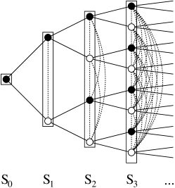
Figure 1. Rooted binary tree with mean-field edges insides spheres and transversely 2-periodic potential.

We call the new (weighted) graph the mean-field binary tree. The spectrum of the mean-field adjacency matrix, $\Delta_{\gamma}^{\mathrm{mf}}$, is the union of two intervals $[-2\sqrt{2}+\gamma,2\sqrt{2}+\gamma]\cup[-2\sqrt{2},2\sqrt{2}]$ and is purely ac. This can be seen by using a Haar basis [11].

For simplicity, we considered a random potential that is transversely two-periodic and defined by the product of two independent Bernoulli measures for $q_{1}$ and $q_{2}$,

$$d\nu(q_{1},q_{2})=\frac{1}{4}\big{(}\delta(q_{1}-1)+\delta(q_{1}+1)\big{)}\big{(}\delta(q_{2}-1)+\delta(q_{2}+1)\big{)}\,.$$ (7.11)

Then we have the following theorem.

Theorem 7.2 (​​[11], Theorem 9).

Let $\nu_{(0)}$ be a probability measure of bounded support for the potential at the root and $\nu$ be the product of Bernoulli measures defined above and let $H_{a,\gamma}:=-\Delta_{\gamma}^{\mathrm{mf}}+a\,q$ be the random discrete Schrödinger operator on the mean-field binary tree corresponding to the transversely two-periodic potential defined by the scaled distribution $\nu_{a}$ and weight $\gamma$. There exist $0<\lambda_{0},\lambda_{1}<2\sqrt{2}$ such that for sufficiently small $a$ the spectral measure for $H_{a}$ corresponding to $\delta_{0}$ has purely ac spectrum in $\{\lambda:|\lambda|\leq\lambda_{0},|\lambda-\gamma|\leq\lambda_{1}\}$.

In this theorem, the constant $\lambda_{0}$ has the same value as in Theorem 6.1, while $\lambda_{1}$ can be taken to be any positive number less than $2\sqrt{2}$.