Modelling Information Flows in Financial Markets

Abstract

This paper presents an overview of information-based asset pricing. In the information-based approach, an asset is defined by its cash-flow structure. The market is assumed to have access to “partial” information about future cash flows. Each cash flow is determined by a collection of independent market factors called $X$-factors. The market filtration is generated by a set of information processes, each of which carries information about one of the $X$-factors, and eventually reveals the $X$-factor in a way that ensures that the associated cash flows have the correct measureability properties. In the models considered each information process has two terms, one of which contains a “signal” about the associated $X$-factor, and the other of which represents “market noise”. The existence of an established pricing kernel, adapted to the market filtration, is assumed. The price of an asset is given by the expectation of the discounted cash flows in the associated risk-neutral measure, conditional on the information provided by the market. When the market noise is modelled by a Brownian bridge one is able to construct explicit formulae for asset prices, as well as semi-analytic expressions for the prices and greeks of options and derivatives. In particular, option price data can be used to determine the information flow-rate parameters implicit in the definitions of the information processes. One consequence of the modelling framework is a specific scheme of stochastic volatility and correlation processes. Instead of imposing a volatility and correlation model upon the dynamics of a set of assets, one is able to deduce the dynamics of the volatilities and correlations of the asset price movements from more primitive assumptions involving the associated cash flows. The paper concludes with an examination of situations involving asymmetric information. We present a simple model for informed traders and show how this can be used as a basis for so-called statistical arbitrage. Finally, we consider the problem of price formation in a heterogeneous market with multiple agents.

1 Cash flow structures and market factors

In financial markets, the revelation of information is the most important factor in the determination of the price movements of financial assets. When a new piece of information (whether true, partly true, misleading, or bogus) circulates in a financial market, the prices of related assets move in response, and they move again when the information is updated. But how do we build specific models that incorporate the impact of information on asset prices? In this article we present an overview of some of the key issues involved in modelling the flow of information in financial markets, and develop in some detail some elementary models for “information” in various situations. We show how information flow processes, when appropriately modelled, can be used to determine the associated price processes of financial assets. Applications to the pricing of various types of contingent claims will also be indicated. One of the contributions of the present work is to introduce a model for dynamic correlation in the situation where we consider a portfolio of assets. Rather than imposing an artificial correlation structure on the assets under consideration, we are able to infer the correlation structure from more basic assumptions. In the final section of the paper, we make some remarks about statistical arbitrage strategies, and about price formation in markets characterised by inhomogeneous information flows.

When models are constructed for the pricing and risk management of complicated financial products, the price dynamics of the simpler financial assets, upon which the more complicated products are based, are often simply “assumed” (modulo some parametric or functional freedom). One can understand from a practical angle why it can be expeditious to proceed on that basis. Nevertheless, from a fundamental view we have to consider that even the basic financial assets (shares, bonds, etc) are characterised by a number of potentially “complex” features, and so to make sense of the behaviour of such assets we need to consider what goes into the determination of their prices. To build up models for the dynamics of asset prices, it seems logical to proceed step by step along the following lines: (1) model the cash-flows arising from the asset as random variables; (2) model the market filtration (the flow of information to the market); (3) model the pricing kernel (which takes into account discounting, risk aversion, and the absence of arbitrage); and (4) work out the resulting dynamics for the price process.

We model the unfolding of chance in a financial market with the specification of a probability space $(\Omega,{\mathcal{F}},\mathbb{P})$ on which we are going to construct a filtration $\{\mathcal{F}_{t}\}$ representing the flow of information to market participants. Here $\mathbb{P}$ denotes the “physical” probability measure. The markets we consider will, in general, be incomplete. That is to say, although derivatives can be priced we do not assume that they can be hedged. Since we are going to model the filtration we say that we are working in an information-based asset pricing framework. The general approach that we describe here is that of Brody, Hughston & Macrina [1, 2, 3].

Consider a financial instrument that delivers to its owner a set of random cash flows $\{D_{T_{k}}\}_{k=1,...,n}$ on the dates $\{T_{k}\}_{k=1,...,n}$. For simplicity, we assume that these dates are fixed, and finite in number. The extension to random dates and to an infinite number of dates is straightforward. Let the pricing kernel be denoted $\{\pi_{t}\}$. At time $t$ the value $S_{t}$ of a contract that generates the cash flows $\{D_{T_{k}}\}_{k=1,\dots,n}$ is given by the following valuation formula:

$$S_{t}=\frac{1}{\pi_{t}}\sum^{n}_{k=1}{\mathds{1}}_{\{t<T_{k}\}}{\mathbb{E}}^{{\mathbb{P}}}\left[\pi_{T_{k}}D_{T_{k}}|{\mathcal{F}}_{t}\right].$$ (1.1)

Thus, at time $t$, for each cash flow that has not yet occurred we take its discounted risk-adjusted conditional expectation, and then we form the sum of such expressions to give the total value of the asset.

Sometimes it is maintained that to regard share prices as being entirely determined by expected dividends is incorrect—that other factors come into play as well, such as the value implicit in corporate control, the value of the status of being a shareholder, and so on. In our view such “implicit” dividends, to the extent that they are relevant, and can be assigned a value, have to be modelled, and thus enter the valuation formula alongside the tangible cash flows. Sometimes it is argued that market sentiment is also important: indeed, it clearly is; but our view is that sentiment is implicit in the imperfect information the market is receiving concerning future cash flows; that sentiment about a future share price is, in essence, information concerning cash flows (both tangible and intangible) extending beyond the date or dates to which the sentiment refers.

In order to apply the valuation formula we need to model the market filtration $\{{\mathcal{F}}_{t}\}$, as well as the pricing kernel $\{\pi_{t}\}$. In particular, it is logical to model the filtration first since the pricing kernel has to be adapted to the filtration. To model the filtration we proceed as follows. Let us introduce a set of independent random variables $\{X_{T_{k}}\}_{k=1,\ldots,n}$, which we call market factors or simply “$X$-factors”. For each $k$, the cash flow $D_{T_{k}}$ is assumed to depend on the market factors $X_{T_{1}},X_{T_{2}},\cdots,X_{T_{k}}$. Thus, in association with each date $T_{k}$ we introduce a so-called “cash-flow function” $\Delta_{T_{k}}$ such that

$$D_{T_{k}}=\Delta_{T_{k}}(X_{T_{1}},X_{T_{2}},\cdots,X_{T_{k}}).$$ (1.2)

For each asset, we need to model the $X$-factors, the a priori probabilities, and the cash-flow functions. In general, the $X$-factor associated with a given date will be a vectorial quantity. The cash-flow diagram associated with a typical asset is illustrated schematically in Figure 1.

Figure 1: The value $S_{t}$ at time $t$ of a security that delivers the random cash flows $D_{T_{1}},D_{T_{2}},\cdots$, at times $T_{1},T_{2},\cdots$, is determined by the valuation formula (1.1). The cash flow $D_{T_{1}}$ is determined by a set of one or more independent $X$-factors $\{X_{T_{1}}\}$. Then $D_{T_{2}}$ is determined by $\{X_{T_{1}},X_{T_{2}}\}$, where $X_{T_{2}}$ represents a further set of independent $X$-factors, and so on.

2 $X$-factor analysis

Let us look at some elementary examples of cash-flow models based on $X$-factors. The first example we consider is a simple credit-risky bond, with two remaining coupons to be paid and no recovery on default. Then we have the following cash-flow structure:

$$D_{T_{1}}={c}X_{T_{1}},$$ (2.1)

$$D_{T_{2}}=({c}+{n})X_{T_{1}}X_{T_{2}}.$$ (2.2)

Here ${c}$ and $n$ denote the coupon and principal, respectively; and $X_{T_{1}}$ and $X_{T_{2}}$ are independent digital random variables taking the values $0$ or $1$ with designated a priori probabilities. Evidently, if the first coupon is not paid, then neither will the second. On the other hand, even if $X_{T_{1}}$ takes the value unity, and the first coupon is paid, the second coupon and the principal will not be paid unless $X_{T_{2}}$ also takes the value unity.

The second example is a simple model for a credit-risky coupon bond with recovery. In this case the cash-flow functions are given as follows:

$$D_{T_{1}}={c}X_{T_{1}}+R_{1}({c}+{n})(1-X_{T_{1}}),$$ (2.3)

$$D_{T_{2}}=({c}+{n})X_{T_{1}}X_{T_{2}}+R_{2}({c}+{n})X_{T_{1}}(1-X_{T_{2}}).$$ (2.4)

Here $R_{1}$ and $R_{2}$ denote recovery rates. Thus if default occurs at the first coupon, then both the coupon and principal become immediately due, and a fixed fraction $R_{1}$ of ${c}+{n}$ is paid. But if default occurs at the second coupon date then the recovery rate is $R_{2}$. We observe that the $X$-factor method allows for a rather transparent representation of the cash-flow structure of such a security, and isolates the variables that underlie the various cash flows.

3 Information processes

We assume that with reference to each market factor market participants will have access to information, which in general is imperfect. We model the imperfect information available to market participants concerning a typical market factor $X_{T}$ with the introduction of a so-called “information process” $\{\xi_{tT}\}_{0\leq t\leq T}$. An information process is required to have the property

$$\xi_{TT}=f(X_{T})$$ (3.1)

for some invertible function $f(x)$. This condition ensures that the information process “reveals” the value of the associated market factor $X_{T}$ at time $T$. At earlier times, the value of $\xi_{tT}$ contains “partial information” about the value of the $X$-factor. We shall come to some explicit examples of information processes shortly.

We are now in a position to say how we model the market filtration. In particular, we shall assume that $\{{\mathcal{F}}_{t}\}$ is generated collectively by the various market information processes $\{\xi_{tT_{k}}\}_{k=1,\ldots,n}$. In other words, the information at time $t$ is given by the following sigma-algebra:

$${\mathcal{F}}_{t}={\sigma}\left[\left\{\xi_{sT_{k}}\right\}_{0\leq s\leq t,\ k=1,...,n}\right].$$ (3.2)

We thus have the following sequence of ideas: market participants are concerned with cash flows; cash flows are dependant on a set of independent market factors; market participants have partial access to the market factors; and this imperfect information generates the market filtration.

We are left with the problem of taking the conditional expectation of the risk-adjusted discounted cash flows to generate price processes; for this purpose we have to model the pricing kernel. We assume that the pricing kernel is adapted to the market filtration. Thus from knowledge of the history of the information processes from time $0$ up to time $t$ one can work out the value of the pricing kernel at $t$ (see, e.g., [8]). In a typical model the pricing kernel is given by the discounted marginal utility of consumption of a representative agent. It is reasonable to suppose that the consumption plan of the agent is adapted to the information filtration. The idea is that the filtration represents the flow of information available at each time $t$ about the relevant market factors, and that the consumption of the agent is determined by this information. In other words, the agent behaves “rationally”, always acting optimally on the available information, in accordance with appropriate criteria. There may be an idiosyncratic element to any given agent’s consumption plan that is not adapted to the market filtration, and is essentially private. But the representative agent has no idiosyncratic consumption.

4 Brownian-bridge information

For the construction of explicit models it is useful to transform to the risk-neutral measure ${\mathbb{Q}}$. This can be achieved by use of the pricing kernel, which we regard as specified. Thus for the present we confine the discussion to “microeconomic” issues: we take no notice of the informational notions implicit in the formulation of the pricing kernel, and make the additional simplifying assumption in what follows that the default-free interest-rate system is deterministic. Then the valuation formula takes the following form:

$$S_{t}=\sum^{n}_{k=1}{\mathds{1}}_{\{t<T_{k}\}}P_{tT_{k}}{\mathbb{E}}^{{\mathbb{Q}}}\left[D_{T_{k}}|{\mathcal{F}}_{t}\right].$$ (4.1)

Absence of arbitrage implies that the discount bond system $\{P_{tT}\}_{0\leq t\leq T<\infty}$ is of the form $P_{tT}=P_{0T}/P_{0t}$, where $\{P_{0t}\}_{0\leq t<\infty}$ is the initial term structure.

With these assumptions in place, we are in a position to specify a model for the information flow. For each $X$-factor $X_{T}$ we take the associated information process to be of the form

$$\xi_{tT}=\sigma tX_{T}+\beta_{tT}.$$ (4.2)

Here $\{\beta_{tT}\}$ is a ${\mathbb{Q}}$-Brownian bridge over the interval $[0,T]$, satisfying $\beta_{0T}=0$, $\beta_{TT}=0$, ${\mathbb{E}}[\beta_{tT}]=0$, and ${\mathbb{E}}\left[\beta_{sT}\beta_{tT}\right]=s(T-t)/T$. The $X$-factor and the Brownian bridge are assumed to be ${\mathbb{Q}}$-independent. Thus the Brownian bridge represents “market noise” and only the “market signal” term involving the $X$-factor contains true market information. The parameter $\sigma$ can be interpreted as the “information flow rate” for the factor $X_{T}$.

In the situation where we have a multiplicity of factors $X_{T_{k}}$ ($k=1,\ldots,n$), the information processes are taken to be of the form

$$\xi_{tT_{k}}=\sigma_{k}tX_{T_{k}}+\beta_{tT_{k}},$$ (4.3)

where we assume that the $X$-factors and Brownian bridges are independent.

The motivation for the use of a bridge to represent noise is intuitively as follows. We assume that initially all available market information is taken into account in the determination of prices, or, equivalently, the a priori probability laws for the market factors. After the passage of time, new stories circulate, and we model this by taking into account that the variance of the Brownian bridge increases for the first half of its trajectory. Eventually, the variance falls to zero at $T$, when the “moment of truth” arrives. The parameter $\sigma$ represents the rate at which the true value of $X_{T}$ is “revealed” as time progresses. Thus, if $\sigma$ is low, then $X_{T}$ is effectively hidden until near the time $T$; on the other hand, if $\sigma$ is high, then we can think of $X_{T}$ as being revealed quickly. If the $X$-factor is “dimensionless”, then $\sigma$ has the units

$$\sigma\sim[{\rm time}]^{-1/2},$$ (4.4)

and a rough measure for the timescale $\tau$ over which information is revealed is

$$\tau=\frac{1}{\sigma^{2}\,{\rm Var}[X_{T}]}.$$ (4.5)

In particular, if $\tau\ll T$, then the value of $X_{T}$ will be revealed rather early, e.g., after the passage of a few multiples of $\tau$. On the other hand, if $\tau\gg T$, then $X_{T}$ will only be revealed at the last minute, as a “surprise”.

We remark that the information process (4.2) has the Markov property. This feature implies simplifications in the resulting models. In particular, on account of the relation (3.1) we find that the conditioning with respect to ${\mathcal{F}}_{t}$ in (4.1) can be replaced by conditioning with respect to the random variables $\xi_{tT_{k}}$ ($k=1,\ldots$). For a proof of the Markov property, see [1, 9].

5 Assets paying a single dividend

Consider an asset that pays single dividend $D_{T}\geq 0$ at time $T$, and assume that there is only one market factor $X_{T}$, so $D_{T}=f(X_{T})$. For the moment, let us assume further that $f(x)=x$. Thus, we have $D_{T}=X_{T}$, where the market factor $X_{T}$ is a continuous nonnegative random variable with a priori ${\mathbb{Q}}$-density $p(x)$ for $x>0$. It follows by use of the Markov property of $\{\xi_{tT}\}$ that the price of such an asset can be written in the form

$$S_{t} = P_{tT}{\mathbb{E}}\left[D_{T}|\xi_{tT}\right]$$ (5.1)

$$= P_{tT}\int_{0}^{\infty}x\,p_{t}(x)\,\mbox{$\rm d$}x,$$

where $p_{t}(x)$ is the conditional density of $X_{T}$. Making use of the the Bayes formula one can show that $p_{t}(x)$ is given more explicitly by

$$p_{t}(x)=\frac{p(x)\exp\left[\frac{T}{T-t}(\sigma x\xi_{tT}-\tfrac{1}{2}\sigma^{2}x^{2}t)\right]}{\int^{\infty}_{0}p(x)\exp\left[\frac{T}{T-t}(\sigma x\xi_{tT}-\tfrac{1}{2}\sigma^{2}x^{2}t)\right]\mbox{$\rm d$}x}.$$ (5.2)

Thus at each time $t<T$ the price of the asset is determined by the random value of the information $\xi_{tT}$ available at that time, and is given by

$$S_{t}=P_{tT}\,\frac{\int_{0}^{\infty}xp(x)\exp\left[\frac{T}{T-t}(\sigma x\xi_{tT}-\tfrac{1}{2}\sigma^{2}x^{2}t)\right]\mbox{$\rm d$}x}{\int^{\infty}_{0}p(x)\exp\left[\frac{T}{T-t}(\sigma x\xi_{tT}-\tfrac{1}{2}\sigma^{2}x^{2}t)\right]\mbox{$\rm d$}x}$$ (5.3)

The dynamics of the price process can then be obtained by an application of Ito’s lemma, with the following result:

$$\mbox{$\rm d$}S_{t}=r_{t}S_{t}\mbox{$\rm d$}t+P_{tT}\frac{\sigma T}{T-t}\,\textrm{Var}_{t}\left[X_{T}\right]\mbox{$\rm d$}W_{t}.$$ (5.4)

Here

$$\textrm{Var}_{t}\left[X_{T}\right]=\int_{0}^{\infty}x^{2}p_{t}(x)\mbox{$\rm d$}x-\left(\int_{0}^{\infty}xp_{t}(x)\mbox{$\rm d$}x\right)^{2}$$ (5.5)

denotes the conditional variance of $X_{T}$, which by (5.2) is evidently given as a function of $t$ and $\xi_{tT}$. The $\{{\mathcal{F}}_{t}\}$-adapted process $\{W_{t}\}$ driving the dynamics of the asset in (5.4) above is not given exogenously, but rather is defined in terms of the information process itself for $t<T$ by the following formula:

$$W_{t}=\xi_{tT}-\int^{t}_{0}\frac{1}{T-s}\left(\sigma T{\mathbb{E}}_{s}\left[X_{T}\right]-\xi_{sT}\right)\mbox{$\rm d$}s.$$ (5.6)

Indeed, one can verify, by use of the Lévy criterion, that the process $\{W_{t}\}$, as thus defined, is an $\{{\mathcal{F}}_{t}\}$-Brownian motion. Hence we see that in an information-based approach we can derive the Brownian motions that drive the markets: they are not “inputs” to the model, but rather can be seen as arising as a “consequence” of the model.

6 Geometric Brownian motion model

A simple application of the $X$-factor technique arises in the case of geometric Brownian motion models. We consider a limited-liability company that makes a single cash distribution $S_{T}$ at time $T$. Alternatively, think of a portfolio containing a single stock which will be sold off at time $T$ for $S_{T}$, with the proceeds of the sale going to the investor. We assume that $S_{T}$ has a log-normal distribution under ${\mathbb{Q}}$, and can be written in the form

$$S_{T}=S_{0}\exp\left(rT+\nu\sqrt{T}X_{T}-\mbox{$\textstyle\frac{1}{2}$}\nu^{2}T\right),$$ (6.1)

where the market factor $X_{T}$ is normally distributed with mean zero and variance one, and where $r>0$ and $\nu>0$ are constants. The information process $\{\xi_{t}\}$ is taken to be of the form (4.2), where in the present example the information flow rate is given by

$$\sigma=\frac{1}{\sqrt{T}}.$$ (6.2)

By use of the Bayes formula we find that the conditional probability density is Gaussian,

$$p_{t}(x)=\sqrt{\frac{T}{2\pi(T-t)}}\,\exp\left(-\frac{1}{2(T-t)}\left(\sqrt{T}x-\xi_{tT}\right)^{2}\right),$$ (6.3)

and has the following dynamics:

$$\mbox{$\rm d$}p_{t}(x)=\frac{1}{T-t}\,\left(\sqrt{T}x-\xi_{tT}\right)p_{t}(x)\mbox{$\rm d$}\xi_{tT}.$$ (6.4)

A short calculation then shows that the value of the asset in this example is given at time $t<T$ by

$$S_{t} = \mbox{$\rm e$}^{-r(T-t)}{\mathbb{E}}_{t}[S_{T}]$$ (6.5)

$$= \mbox{$\rm e$}^{-r(T-t)}\int_{-\infty}^{\infty}S_{0}\mbox{$\rm e$}^{rT+\nu\sqrt{T}x-\frac{1}{2}\,\nu^{2}T}p_{t}(x)\mbox{$\rm d$}x$$

$$= S_{0}\exp\left(rt+\nu\xi_{tT}-\mbox{$\textstyle\frac{1}{2}$}\nu^{2}t\right).$$

The surprising fact is that $\{\xi_{tT}\}$ itself turns out to be an $\{{\mathcal{F}}_{t}\}$-Brownian motion. Hence, writing $W_{t}=\xi_{tT}$ for $0\leq t\leq T$ we obtain the standard geometric Brownian motion model:

$$S_{t}=S_{0}\exp\left(rt+\nu W_{t}-\mbox{$\textstyle\frac{1}{2}$}\nu^{2}t\right).$$ (6.6)

We see that starting with an information-based argument we are able to recover the familiar asset price dynamics given by (6.6). An important point to note is that the Brownian bridge process $\{\beta_{tT}\}$ arises naturally in this context. In fact, if we start with (6.6) then we can make use of the following well-known orthogonal decomposition:

$$W_{t}=\frac{t}{T}\,W_{T}+\left(W_{t}-\frac{t}{T}\,W_{T}\right).$$ (6.7)

The second term on the right, which is independent of the first term on the right, is a standard representation for a Brownian bridge process:

$$\beta_{tT}=W_{t}-\frac{t}{T}\,W_{T}.$$ (6.8)

Then by setting $X_{T}=W_{T}/\sqrt{T}$ and $\sigma=1/\sqrt{T}$ we find that the right side of (6.7) is indeed the market information. In other words, when it is formulated in an information-based framework, the standard Black-Scholes-Merton theory can be expressed in terms of a normally distributed $X$-factor and an independent Brownian-bridge noise process.

7 Pricing contingent claims

The information-based price (5.3) of a single-dividend paying asset at first glance appears to be given by a rather complicated expression, suggesting perhaps that it would be impractical for use as a model for the pricing and hedging of contingent claims. However, there is a remarkable simplification involving a change of measure that allows one both to price and to hedge vanilla options. This can be seen as follows. Let us consider a European-style call option on the asset, with option maturity $t$ and strike $K$. The value of the option at time $0$ is given by

$$C_{0}=P_{0t}{\mathbb{E}}^{\mathbb{Q}}\left[(S_{t}-K)^{+}\right].$$ (7.1)

Let us define a process $\{\Phi_{t}\}$ by the expression appearing in the denominator of (5.3), so

$$\Phi_{t}=\int^{\infty}_{0}p(x)\exp\left[\frac{T}{T-t}(\sigma x\xi_{tT}-\tfrac{1}{2}\sigma^{2}x^{2}t)\right]\mbox{$\rm d$}x.$$ (7.2)

Then it can be shown that $\{\Phi_{t}^{-1}\}$ is a positive ${\mathbb{Q}}$-martingale, which can be used to change the probability measure from ${\mathbb{Q}}$ to a new measure ${\mathbb{B}}$. Under the measure ${\mathbb{B}}$, which we call the “bridge measure”, the information process itself is a Brownian bridge. More precisely, under ${\mathbb{B}}$ the process $\{\xi_{sT}\}_{0\leq s\leq t}$ has the law of a Brownian bridge spanning the interval $[0,T]$, restricted to $[0,t]$. That is to say, $\{\xi_{sT}\}_{0\leq s\leq t}$ is ${\mathbb{B}}$-Gaussian with mean zero and covariance ${\rm cov}[\xi_{aT},\xi_{bT}]=a(T-b)/T$ for $0\leq a\leq b\leq t$. The initial value of the option is thus given by

$$C_{0} = P_{0t}{\mathbb{E}}^{\mathbb{B}}\left[\left(P_{tT}\int^{\infty}_{0}\!\!xp(x)\mbox{$\rm e$}^{\frac{T}{T-t}(\sigma x\xi_{tT}-\frac{1}{2}\sigma^{2}x^{2}t)}\mbox{$\rm d$}x\right.\right.$$ (7.3)

$$\qquad\qquad\left.\left.-K\int^{\infty}_{0}\!\!p(x)\mbox{$\rm e$}^{\frac{T}{T-t}(\sigma x\xi_{tT}-\frac{1}{2}\sigma^{2}x^{2}t)}\mbox{$\rm d$}x\right)^{+}\right].$$

It can be shown that the asset price is a monotonically increasing function of the value of $\xi_{tT}$. It follows that there is a unique critical level $\xi^{*}$ for the information such that the expression inside the max-function in (7.3) is positive. It follows that the option price can be written in terms of a single integration involving the normal distribution function:

$$C_{0}=P_{0t}\int_{0}^{\infty}p(x)\left(P_{tT}x-K\right)N\left(\frac{\xi^{*}-\sigma xt}{\sqrt{t(T-t)/T}}\right)\mbox{$\rm d$}x.$$ (7.4)

As another example we consider the following. Suppose that the single cash flow $D_{T}$ is a binary random variable taking the values $\{d_{0},d_{1}\}$ with a priori probabilities $\{p_{0},p_{1}\}$. The asset in this case can be thought of as a simple credit-risky discount bond that pays $d_{1}$ if there is no default, and $d_{0}$ if there is a default. A short calculation allows one to verify that

$$C_{0}=P_{0t}\Big{[}p_{1}(P_{tT}d_{1}-K)N(u^{+})-p_{0}(K-P_{tT}d_{0})N(u^{-})\Big{]},$$ (7.5)

where $u^{+}$ and $u^{-}$ are defined by

$$u^{\pm}=\frac{\ln\left[\frac{p_{1}(P_{tT}d_{1}-K)}{p_{0}(K-P_{tT}d_{0})}\right]\pm\tfrac{1}{2}\sigma^{2}(d_{1}-d_{0})^{2}\tau}{\sigma\sqrt{\tau}(d_{1}-d_{0})},$$ (7.6)

with $\tau=tT/(T-1)$. It can be shown that the option delta at time $0$, defined as usual by

$$\delta_{0}=\frac{\partial C_{0}}{\partial S_{0}},$$ (7.7)

can be calculated explicitly, with the following result:

$$\delta_{0}=\frac{(P_{tT}d_{1}-K)N(u^{+})+(K-P_{tT}d_{0})N(u^{-})}{P_{tT}(d_{1}-d_{0})}.$$ (7.8)

We see, therefore, that the apparent complexity of (5.3) does not lead to any intractability when it comes to derivatives pricing and hedging.

8 Volatility and correlation

In the case of an asset that pays multiple dividends, the price is determined by the conditional expectation given in equation (4.1). In terms of the cash-flow functions defined by (1.2) we thus obtain the following for the dynamics of the asset price:

$$\mbox{$\rm d$}S_{t} = r_{t}\,S_{t}\,\mbox{$\rm d$}t+\sum_{k=1}^{n}\Delta_{T_{k}}\mbox{$\rm d$}{\mathds{1}}_{\{t<T_{k}\}}$$ (8.1)

$$+\sum^{n}_{k=1}{\mathds{1}}_{\{t<T_{k}\}}\,P_{tT_{k}}\sum^{k}_{j=1}\frac{\sigma_{j}T_{j}}{T_{j}-t}\,{\rm Cov}_{t}\left[\Delta_{T_{k}},X_{T_{j}}\right]\mbox{$\rm d$}W^{j}_{t}.$$

The leading term in the drift is the short rate, as one might expect, and there is also a term representing the downward jump in the asset that occurs when a dividend is paid. The independent $\{{\mathcal{F}}_{t}\}$-adapted Brownian motions $\{W^{j}_{t}\}$ driving the price dynamics are given in terms of the corresponding information processes by

$$W^{j}_{t}=\xi_{tT_{j}}-\int^{t}_{0}\frac{1}{T_{j}-s}\left(\sigma_{j}\,T_{j}\,{\mathbb{E}}_{s}\left[X_{T_{j}}\right]-\xi_{sT_{j}}\right)\mbox{$\rm d$}s.$$ (8.2)

We see that if an asset delivers one or more cash flows depending on two or more market factors, then it will exhibit “unhedgeable” stochastic volatility [2, 7]. That is to say, one would not expect to be able to hedge a position in an option by use of a position in the underlying. In general, if the asset cash flows depend on $n$ $X$-factors in total, then to hedge a generic derivative based on the given asset one will need the underlying together with $n-1$ options as hedging instruments, i.e. $n$ hedging instruments in total. One can read from (8.1) the generic form of the stochastic volatility implied for a given configuration of $X$-factors and cash-flow functions.

It follows likewise from (8.1) that two or more assets will exhibit dynamic correlation when they share one or more $X$-factors in common. As a specific example of dynamic correlation let us consider a pair of credit-risky discount bonds. The first bond is defined by a cash flow $D_{T_{1}}$ at $T_{1}$. The second is defined by a cash flow $D_{T_{2}}$ at $T_{2}>T_{1}$. The cash flow structure is taken to be:

$$D_{T_{1}}={n}_{1}X_{T_{1}}+R_{1}{n}_{1}(1-X_{T_{1}}),$$ (8.3)

and

$$D_{T_{2}} = {n}_{2}X_{T_{1}}X_{T_{2}}+R^{a}_{2}{n}_{2}(1-X_{T_{1}})X_{T_{2}}$$ (8.4)

$$+R^{b}_{2}{n}_{2}X_{T_{1}}(1-X_{T_{2}})+R^{c}_{2}{n}_{2}(1-X_{T_{1}})(1-X_{T_{2}}).$$

Here, ${n}_{1}$ and ${n}_{2}$ denote the bond principals, and $X_{T_{1}}$ and $X_{T_{2}}$ are independent digital random variables. The possible recovery rates in the case of default are denoted by $R_{1}$, $R^{a}_{2}$, $R^{b}_{2}$, and $R^{c}_{2}$. One can have in mind the following story. Consider a factory with debt $S_{t}^{1}$. Across the street is a little restaurant with debt $S_{t}^{2}$. If the factory goes bust ($X_{T_{1}}=0$) then so will the restaurant, because this is where the workers have their lunch. On the other hand, even if the factory is successful ($X_{T_{1}}=1$), the restaurant may still go bust on account of bad management ($X_{T_{2}}=0$). The recovery rates on the restaurant bond depend on the details of what goes wrong: $R^{a}_{2}$ (restaurant fails because factory fails); $R^{b}_{2}$ (restaurant fails on account of bad management); $R^{c}_{2}$ (factory fails, and bad restaurant management). One might expect $R^{b}_{2}>R^{a}_{2}$, since as long as the factory continues, the restaurant facilities could be sold at a good price. The worst scenario is that of $R^{c}_{2}$. For the dynamics of the first bond (the “factory”), for which the price is

$$S^{1}_{t}=P_{tT_{1}}{\mathbb{E}}_{t}\left[D_{T_{1}}\right],\qquad(t<T_{1}),$$ (8.5)

we have:

$$\mbox{$\rm d$}S^{1}_{t}=r_{t}S^{1}_{t}\mbox{$\rm d$}t+P_{tT_{1}}\frac{\sigma_{1}T_{1}}{T_{1}-t}\,\alpha\,\textrm{Var}_{t}\left[X_{T_{1}}\right]\mbox{$\rm d$}W^{1}_{t},$$ (8.6)

where $\alpha={n}_{1}(1-R_{1})$. For the dynamics of the second bond (the “restaurant”), for which the price is

$$S^{2}_{t}=P_{tT_{2}}{\mathbb{E}}_{t}\left[D_{T_{2}}\right],\qquad(t<T_{2}),$$ (8.7)

we have:

$$\mbox{$\rm d$}S^{2}_{t} = r_{t}S^{2}_{t}\mbox{$\rm d$}t+P_{tT_{2}}\frac{\sigma_{1}T_{1}}{T_{1}-t}\left(\beta+\delta{\mathbb{E}}_{t}\left[X_{T_{2}}\right]\right)\textrm{Var}_{t}\left[X_{T_{1}}\right]\mbox{$\rm d$}W^{1}_{t}$$ (8.8)

$$+P_{tT_{2}}\frac{\sigma_{2}T_{2}}{T_{2}-t}\left(\gamma+\delta{\mathbb{E}}_{t}\left[X_{T_{1}}\right]\right)\textrm{Var}_{t}\left[X_{T_{2}}\right]\mbox{$\rm d$}W^{2}_{t},$$

where the constants $\beta$, $\gamma$, and $\delta$ are given by $\beta={n}_{2}(R^{b}_{2}-R^{c}_{2})$, $\gamma={n}_{2}(R^{a}_{2}-R^{c}_{2})$, and $\delta={n}_{2}(1-R^{a}_{2}-R^{b}_{2}+R^{c}_{2})$. The filtration $\{{\mathcal{F}}_{s}\}$ is generated by the information processes $\{\xi_{sT_{1}}\}$ and $\{\xi_{sT_{2}}\}$ associated with $X_{T_{1}}$ and $X_{T_{2}}$. The dynamics of the bond prices depend on a common Brownian driver $\{W^{1}_{t}\}$. The fact that the asset payoffs share a common $X$-factor thus gives rise to a dynamic correlation between the movements of the price processes $\{S^{1}_{t}\}$ and $\{S^{2}_{t}\}$. The instantaneous correlation between the price movements of the factory bond and the restaurant bond is given by the following expression:

$$\rho_{t}=\frac{\mbox{$\rm d$}S^{1}_{t}\,\mbox{$\rm d$}S^{2}_{t}}{\sqrt{\big{(}\mbox{$\rm d$}S^{1}_{t}\big{)}^{2}\big{(}\mbox{$\rm d$}S^{2}_{t}\big{)}^{2}}}.$$ (8.9)

Hence, using the formulae for the dynamics of the two assets, we obtain:

$$\rho_{t}=\frac{1}{\sqrt{\psi_{t}}}\frac{\sigma_{1}T_{1}}{T_{1}-t}\left(\beta+\delta{\mathbb{E}}_{t}\left[X_{T_{1}}\right]\right){\rm Var}_{t}\left[X_{T_{1}}\right],$$ (8.10)

where

$$\psi_{t} = \left(\frac{\sigma_{1}T_{1}}{T_{1}-t}\right)^{2}\left(\beta+\delta\,{\mathbb{E}}_{t}\left[X_{T_{2}}\right]\right)^{2}\left({\rm Var}_{t}\left[X_{T_{1}}\right]\right)^{2}$$ (8.11)

$$+\left(\frac{\sigma_{2}T_{2}}{T_{2}-t}\right)^{2}\left(\gamma+\delta\,{\mathbb{E}}_{t}\left[X_{T_{1}}\right]\right)^{2}\left({\rm Var}_{t}\left[X_{T_{2}}\right]\right)^{2}.$$

We see from (8.10) that we are able to calculate explicitly the dynamics of the correlation between the movements of the two asset prices.

9 Amount of information about the future cash flow contained in the price process

Since we are modelling the flow of information in an explicit manner, we are able to quantify how much information regarding the value of the cash flow $D_{T}$ is contained in the value $\xi_{t}$ at time $t$ of the associated information process. For simplicity we shall in the discussion that follows assume that the cash flow $D_{T}$ takes the discrete values $\{d_{i}\}_{i=1,\ldots,n}$ with a priori probabilities $\{p_{i}\}_{i=1,\ldots,n}$. A reasonable measure for quantifying the information content is given by the mutual information $J(\xi_{t},D_{T})$ between the two random variables, which in the present context is given by the expression

$$J(\xi_{t},D_{T})=\sum_{i=1}^{n}\int_{-\infty}^{\infty}\rho(\xi,i)\,\ln\left(\frac{\rho(\xi,i)}{\rho(\xi)\rho(i)}\right)\mbox{$\rm d$}\xi,$$ (9.1)

where

$$\rho(\xi,i)=\frac{\mbox{$\rm d$}}{\mbox{$\rm d$}\xi}\,{\mathbb{Q}}\Big{[}(\xi_{t}<\xi)\cap(D_{T}=d_{i})\Big{]}$$ (9.2)

is the joint density of the random variables $\xi_{t}$ and $D_{T})$, and $\rho(\xi)$ and $\rho(i)$ are the respective marginal probabilities. By use of the relation

$${\mathbb{Q}}\Big{[}(\xi_{t}<\xi)\cap(D_{T}=d_{i})\Big{]}={\mathbb{Q}}(\xi_{t}<\xi|D_{T}=d_{i})\,{\mathbb{Q}}(D_{T}=d_{i})$$ (9.3)

we deduce that

$$\rho(\xi,i)=p_{i}\frac{1}{\sqrt{2\pi t(T-t)/T}}\,\exp\left(-\mbox{$\textstyle\frac{1}{2}$}\frac{(x-\sigma d_{i}t)^{2}}{t(T-t)/T}\right),$$ (9.4)

since conditional on $D_{T}=d_{i}$ the random variable $\xi_{t}$ is normally distributed with mean $\sigma td_{i}$ and variance $t(T-t)/T$. From (9.4) the marginal densities

$$\rho(\xi)=\sum_{i=1}^{n}\rho(\xi,i)\quad{\rm and}\quad\rho(i)=\int_{-\infty}^{\infty}\rho(\xi,i)\mbox{$\rm d$}\xi$$ (9.5)

can be deduced. In particular, $\rho(i)=p_{i}$. By substituting (9.4) in (9.1), the information about the cash flow $D_{T}$ contained in $\xi_{t}$ can be determined.

From an information-theoretic point of view, two processes related through an invertible function, thus sharing the same filtration, in general possess different information content. On the other hand, since what is observed in the market is the price $S_{t}$, which is an invertible function of $\xi_{t}$, it is more relevant to determine the mutual information $J(S_{t},D_{T})$, that is, the amount of information about the future cash flow contained in the market price. It can be shown that in the present context we have $J(S_{t},D_{T})=J(\xi_{t},D_{T})$.

10 Information disparity and statistical arbitrage

So far we have assumed that market participants have equal access to information, but one can ask what happens if some traders are more “informed” than others. Suppose we consider a financial product that pays a single cash flow $D_{T}$ at time $T$. We can think of this product as a kind of bond. The general market trader has access to an information process concerning $D_{T}$, but there are also “informed” traders who have access to one or more additional information processes concerning $D_{T}$. The informed trader is thus in some sense able to make a “better estimate” of the value of the asset.

To be more specific, let us suppose that while the general market trader has access to the information $\xi_{t}=\sigma tD_{T}+\beta_{tT}$, an informed trader has access in addition, say, to the information $\xi^{\prime}_{t}=\sigma^{\prime}tD_{T}+\beta^{\prime}_{tT}$, where $\{\beta_{tT}^{\prime}\}$ may or may not be correlated with the market noise $\{\beta_{tT}\}$. Thus, the information source for the informed trader is given by $\{{\mathcal{G}}_{t}\}={\sigma}(\{\xi_{s},\xi^{\prime}_{s}\}_{0\leq s\leq t})$. The use of such extra information can, but need not, represent “insider trading” in the usual sense. That is, it may be that the informed trader merely has better access to (and better computer power for the purpose of digesting) the vast domain of publicly available information. Since we have introduced an information measure regarding impending cash flows, we can quantify the excess information held by the informed trader above that held by general market traders. This is measured by the difference of the mutual information $\Delta J$. In figure 2 we plot an example of $\Delta J$, indicating the way in which the excess information held by the informed trader changes in time.

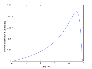
Figure 2: Mutual information difference. The additional information held by an informed trader over that of the market is nonnegative. The parameters are set to be $d_{1}=0$, $d_{2}=1$, $p_{1}=0.2$, $p_{2}=0.8$, $T=5$, $\sigma=0.25$, $\sigma^{\prime}=0.45$, and $\rho=0.15$ (the correlation between $\beta_{tT}$ and $\beta^{\prime}_{tT}$).

Given that the informed trader is on average “more knowledgeable” than the general market trader, it is natural to ask how the informed trader can take advantage of the situation to seek so-called “statistical arbitrage” opportunities. We assume that the informed trader operates on a relatively small scale, and that the actions of this trader do not significantly influence the market. Suppose we consider a trading strategy such that at some designated time $t\in(0,T)$ a market trader purchases a bond if, and only if, at that time the bond price $S_{t}$ is greater than the quantity $KP_{tT}$ for some specified constant $K$. Once a bond is purchased, it is held to maturity. The informed trader follows the same rule, but makes a better estimate of the value of the bond, and hence purchases the bond iff ${\tilde{S}}_{t}>KP_{tT}$, where

$${\tilde{S}}_{t}=P_{tT}{\mathbb{E}}[D_{T}|{\mathcal{G}}_{t}].$$ (10.1)

The significance of ${\tilde{S}}_{t}$ is that it represents the price that the informed trader knows that the market as a whole would make if the market as a whole had the same knowledge as the informed trader.

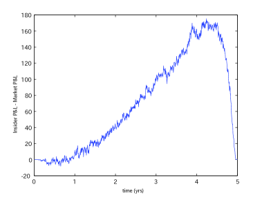
Figure 3: The P&L difference for digital bonds. At each time traders purchase the bond if and only if the valuation of the bond is greater than a specified threshold. The general market trader buys if $S_{t}>KP_{tT}$, whereas the informed trader uses the criterion ${\tilde{S}}_{t}>KP_{tT}$. The difference in profit and loss between the informed trader and the general market trader is plotted, based on $2000$ realisations, when the a priori probability of default is $p_{1}=0.2$. Other parameters are set to be $d_{1}=0$, $d_{2}=1$, $T=5$, $\sigma=0.25$, $\sigma^{\prime}=0.45$, $\rho=0.15$, and $K=0.7$.

That such a strategy leads to a statistical arbitrage opportunity for the informed trader can be seen as follows [4]. We assume that the initial position of a trader is zero, i.e. purchase of a bond at $t$ requires borrowing the amount $S_{t}$ at that time, and repaying the amount $P_{tT}^{-1}S_{t}$ at $T$. Thus the value of a general market trader’s portfolio at $T$ is

$$V_{T}={\mathds{1}}{\{S_{t}>KP_{tT}\}}(D_{T}-P_{tT}^{-1}S_{t}),$$ (10.2)

whereas the value of the informed trader’s portfolio at $T$ is

$${\tilde{V}}_{T}={\mathds{1}}{\{{\tilde{S}}_{t}>KP_{tT}\}}(D_{T}-P_{tT}^{-1}S_{tT}).$$ (10.3)

Consider the present value $P_{0T}{\mathbb{E}}[\Delta V_{T}]$ of a security that delivers a cash flow equal to the excess profit or loss

$$\Delta V_{T}={\tilde{V}}_{T}-V_{T}$$ (10.4)

generated by the strategy of the informed trader. By the tower property we have

$${\mathbb{E}}[\Delta V_{T}]={\mathbb{E}}[{\mathbb{E}}[\Delta V_{T}|{\mathcal{G}}_{t}]].$$ (10.5)

However,

$${\mathbb{E}}[\Delta V_{T}|{\mathcal{G}}_{t}]=P_{tT}^{-1}\left({\mathds{1}}{\{{\tilde{S}}_{t}>KP_{tT}\}}-{\mathds{1}}{\{S_{t}>KP_{tT}\}}\right)\left({\tilde{S}}_{t}-S_{t}\right),$$ (10.6)

since the random variables $S_{t}$ and ${\tilde{S}}_{t}$ are ${\mathcal{G}}_{t}$-measurable. If ${\tilde{S}}_{t}>S_{t}$ then

$${\mathds{1}}{\{{\tilde{S}}_{t}>KP_{tT}\}}-{\mathds{1}}{\{S_{t}>KP_{tT}\}}\geq 0;$$ (10.7)

whereas if ${\tilde{S}}_{t}<S_{t}$ then

$${\mathds{1}}{\{{\tilde{S}}_{t}>KP_{tT}\}}-{\mathds{1}}{\{S_{t}>KP_{tT}\}}\leq 0.$$ (10.8)

It follows that ${\mathbb{E}}[\Delta V_{T}|{\mathcal{G}}_{t}]>0$ with probability greater than zero, and therefore ${\mathbb{E}}[\Delta V_{T}]>0$. We know that according to the usual no-arbitrage arguments the present value of the payoff of the strategy of the general market trader must be zero. It follows that the informed trader can execute a transaction at zero cost that has positive value: this is what we mean by “statistical arbitrage”. A simulation study of the profit arising from this trading strategy is shown in figure 3, indicating a close correspondence with the excess information held by the informed trader shown in figure 2.

11 Price formation in inhomogeneous markets

The idea of “informed trading” can be extended to a market that has a number of traders operating in it, all more or less on an equal footing, but where different traders have access to different information. In other words, there is an inhomogeneous information flow in the market. This line of thinking leads naturally to the consideration of price formation in such a market.

Let us consider, as an example, a market with two traders, labelled “Trader 1” and “Trader 2”. As before, there is a single asset, with a single dividend $D_{T}$ paid at time $T$. The traders have access to separate sources of information about $D_{T}$, given respectively by $\xi^{1}_{t}=\sigma_{1}tD_{T}+\beta^{1}_{tT}$ and $\xi^{2}_{t}=\sigma_{2}tD_{T}+\beta^{2}_{tT}$. Here the Brownian bridges $\{\beta_{tT}^{1}\}$ and $\{\beta^{2}_{tT}\}$ are assumed, for simplicity, to be independent. Trader 1 works out the price

$$S_{t}^{1}=P_{tT}{\mathbb{E}}[D_{T}|\xi^{1}_{t}]$$ (11.1)

that he knows the market would have made had the market possessed the information generated by $\{\xi^{1}_{t}\}$. Likewise, Trader 2 works out the price

$$S_{t}^{2}=P_{tT}{\mathbb{E}}[D_{T}|\xi^{2}_{t}]$$ (11.2)

that she knows the market would have made had the market possessed the information generated by $\{\xi^{2}_{t}\}$.

Traders 1 and 2 are unaware of each other’s prices, but can gain information by trading. The trading process works as follows. Each trader makes a spread about their price. Letting $0<\phi^{-}<1<\phi^{+}$, we set

$$S_{t}^{1\pm}=\phi^{\pm}S_{t}^{1}$$ (11.3)

for the buy price $S_{t}^{1-}$ and sell price $S_{t}^{1+}$ made by Trader 1 at time $t$. Thus Trader 1 is willing to buy at a price slightly below his information-based valuation $S_{t}^{1}$, and is willing to sell at a price that is slightly above that valuation. Likewise Trader 2 is willing to buy at a price slightly below her information-based valuation $S_{t}^{2}$, and is willing to sell at a price that is slightly above that valuation:

$$S_{t}^{2\pm}=\phi^{\pm}S_{t}^{2}.$$ (11.4)

We assume that there is an exchange that continuously monitors the prices made by the traders. The exchange effects a trade of some fixed size when the buy price of one of the traders reaches the level of the sell price of the other trader. That is to say, a trade takes place when

$$S_{t}^{1-}=S_{t}^{2+}\quad\textrm{or}\quad S_{t}^{1+}=S_{t}^{2-}.$$ (11.5)

When a trade occurs, at that moment each trader learns the price of the other, and as a consequence can back out the value of the corresponding information process. Therefore, when a trade occurs, the traders each briefly have access to both pieces of information, and are thus in a position to make a better price, namely that given by

$$S_{t}^{1,2}=P_{tT}{\mathbb{E}}[D_{T}|\xi_{t}^{1},\xi^{2}_{t}].$$ (11.6)

We conclude that immediately after a trade the information-based prices made by each of the traders will jump to the same level, and that the a priori probability distribution for $D_{T}$ will be updated correspondingly.

Once the trade is concluded, the link between the two traders is lost, and each trader again has access only to their own information source. Starting from the same price, the prices made by the two traders diverge as they receive different information going forward. A further trade will then occur when the buy price of one of the traders next hits the sell price of the other trader.

At the time the trade is executed, the joint information can be embodied in the value of an effective information process $\{{\hat{\xi}}_{t}\}_{0\leq t\leq T}$ given by

$${\hat{\xi}}_{t}=\sqrt{(\sigma_{1})^{2}+(\sigma_{2})^{2}}\,tD_{T}+\frac{\sigma_{1}\,\beta^{1}_{tT}+\sigma_{2}\,\beta^{2}_{tT}}{\sqrt{(\sigma_{1})^{2}+(\sigma_{2})^{2}}}.$$ (11.7)

We note that $\{{\hat{\xi}}_{t}\}$ is indeed an information process, since it can be written in the form

$${\hat{\xi}}_{t}=\hat{\sigma}tD_{T}+\hat{\beta}_{tT},$$ (11.8)

where

$$\hat{\sigma}=\sqrt{(\sigma_{1})^{2}+(\sigma_{2})^{2}},\quad{\rm and}\quad\hat{\beta}_{tT}=\frac{\sigma_{1}\,\beta^{1}_{tT}+\sigma_{2}\,\beta^{2}_{tT}}{\sqrt{(\sigma_{1})^{2}+(\sigma_{2})^{2}}}.$$ (11.9)

One can show that $\{\hat{\beta}_{tT}\}$ is a Brownian bridge and is independent of $D_{T}$. Thus, immediately after the trade is executed, the price $S^{1,2}_{t}$ made by both traders is of the form

$$S^{1,2}_{t}=P_{tT}\,\frac{\int^{\infty}_{0}x\,p(x)\exp\left[\frac{T}{T-t}\left(\hat{\sigma}\,x\,{\hat{\xi}}_{t}-\tfrac{1}{2}\,\hat{\sigma}^{2}\,x^{2}\,t\right)\right]\mbox{$\rm d$}x}{\int^{\infty}_{0}p(x)\exp\left[\frac{T}{T-t}\left(\hat{\sigma}\,x\,{\hat{\xi}}_{t}-\tfrac{1}{2}\,\hat{\sigma}^{2}\,x^{2}\,t\right)\right]\mbox{$\rm d$}x}.$$ (11.10)

Figure 4: Schematic illustration of information-based trading. An exchange executes a trade when the sell price of Trader $i$ matches the buy price of Trader $j$ (dashed lines meet at filled dots). At the execution time $t_{n}$, both traders have access to each other’s valuations $S^{i}_{t_{n}}$ (empty circles) and thus to each other’s information. As a consequence, the traders are able to update their valuations and obtain the common price $S^{j,k}_{t_{n}}$. After the trade has been executed and the respective asset valuations have been updated, the traders “separate”, and return to their individual valuations. The respective valuations may drift in different directions. The traders will get in contact again as soon as the exchange notifies them that the respective sell and buy prices have matched again. Such an information-based trading mechanism can be extended to multiple traders, as suggested in the illustration.

As an example, let us consider the case of a digital payout taking the values 0 and 1 with a priori probabilities $p_{0}$ and $p_{1}$. We consider the case in which the information flow rates are the same, so we set $\sigma_{1}=\sigma_{2}=\sigma$. Then for the valuations we have

$$S_{t}^{1}=\frac{p_{1}\,\exp\left[\frac{T}{T-t}\left(\sigma\xi^{1}_{t}-\tfrac{1}{2}\,\sigma^{2}t\right)\right]}{p_{0}+p_{1}\,\exp\left[\frac{T}{T-t}\left(\sigma\xi^{1}_{t}-\tfrac{1}{2}\,\sigma^{2}t\right)\right]}$$ (11.11)

and

$$S_{t}^{2}=\frac{p_{1}\,\exp\left[\frac{T}{T-t}\left(\sigma\xi^{2}_{t}-\tfrac{1}{2}\,\sigma^{2}t\right)\right]}{p_{0}+p_{1}\,\exp\left[\frac{T}{T-t}\left(\sigma\xi^{2}_{t}-\tfrac{1}{2}\,\sigma^{2}t\right)\right]}.$$ (11.12)

For the spreads, we assume $\phi^{+}=1+\delta$ and $\phi^{-}=1-\delta$ where $\delta$ is small. If Trader 1 is the buyer then the condition for a trade is

$$(1-\delta)S^{1}_{t}=(1+\delta)S^{2}_{t}.$$ (11.13)

Given his knowledge $\xi^{1}_{t}$, Trader 1 can use the condition to work out the value of $\xi_{t}^{2}$. In particular, suppose that

$$\xi^{2}_{t}=\xi^{1}_{t}+\varepsilon_{t},$$ (11.14)

where $\varepsilon_{t}$ is small. Then a calculation shows that $\varepsilon_{t}$ is given, to first order, by

$$\varepsilon_{t}=-\frac{2\,\delta(T-t)}{\sigma\,T\left(1-{\mathbb{E}}\big{[}X_{T}\,|\,\xi^{1}_{t}\big{]}\right)}.$$ (11.15)

The general situation, where there are a number of traders present in the market, and where the asset cash flows depend on a number of market factors, is very rich. It is evident that in the broad picture there is no universal filtration, nor a universal pricing measure. Nevertheless, by exchanging information through trading activity, market participants can maintain a “law of reasonable price range” if not a “law of one price”.

Certainly, the notion that there is a universal market filtration is unrealistic. What counts is not merely “access in principle” to information, but rather “access in practice”. Perhaps some broader version of market efficiency will survive, taking into account the cost of such access (cf. [5]). A subscription to the Wall Street Journal is not free, nor is a Bloomberg terminal. Access to vast information providers such as Google and Yahoo may seem free or nearly so, but from a broader perspective this is not so—someone pays, in cash or kind. What is the market price of information? And how does this depend on the “information about the information”? For the answers to these questions we must await the development of new models.

Acknowledgements. The authors are grateful to seminar participants at the Fourth General Conference on Advanced Mathematical Methods in Finance, Alesund, Norway, May 2009, the Workshop on Incomplete Information in Mathematical Finance, Chemnitz, Germany, June 2009, the Graduate School of Management, Kyoto, October 2009, and the Kyoto Institute of Economic Research, January 2010, for helpful comments. Part of this work was carried out while LPH was visiting the Aspen Center for Physics (September 2009), and Kyoto University (August, October 2009). DCB and LPH thank HSBC, Lloyds TSB, Shell International, and Yahoo Japan for research support.

References

- [1] D. C. Brody, L. P. Hughston & A. Macrina (2007) “Beyond hazard rates: a new framework for credit-risk modelling” In Advances in Mathematical Finance, Festschrift volume in honour of Dilip Madan. R. Elliott, M. Fu, R. Jarrow and Ju-Yi Yen, eds. (Basel: Birkhäuser).
- [2] D. C. Brody, L. P. Hughston & A. Macrina (2008) “Information-based asset pricing” Int. J. Theor. Appl. Fin. 11, 107-142.
- [3] D. C. Brody, L. P. Hughston & A. Macrina (2008) “Dam rain and cumulative gain” Proc. Roy. Soc. Lond. A464 1801-1822.
- [4] D. C. Brody, M. H. A. Davis, R. L. Friedman & L. P. Hughston (2009) “Informed traders” Proc. Roy. Soc. Lond. A465, 1103-1122.
- [5] S. J. Grossman & J. E. Stiglitz (1980) “On the impossibility of informationally efficient markets” Am. Econ. Rev. 70 393-408.
- [6] L. P. Hughston & A. Macrina (2008) “Information, Inflation, and Interest” In Advances in Mathematics of Finance, Banach Center Publications 83 (Institute of Mathematics, Polish Academy of Sciences).
- [7] A. Macrina (2006) An Information-Based Framework for Asset Pricing: X-factor theory and its Applications. PhD thesis, King’s College London.
- [8] A. Macrina & P. A. Parbhoo (2010) “Securities pricing with information-sensitive discounting” In Recent Advances in Financial Engineering 2009, Proceedings of the KIER-TMU International Workshop on Financial Engineering 2009 (Singapore: World Scientific Publishing).
- [9] M. Rutkowski & N. Yu (2007) “On the Brody-Hughston-Macrina approach to modelling of defaultable term structure” Int. J. Theor. Appl. Fin. 10, 557-589.