The DiskMass Survey. I. Overview

Abstract

We present a survey of the mass surface-density of spiral disks, motivated by outstanding uncertainties in rotation-curve decompositions. Our method exploits integral-field spectroscopy to measure stellar and gas kinematics in nearly face-on galaxies sampled at 515, 660, and 860 nm, using the custom-built SparsePak and PPak instruments. A two-tiered sample, selected from the UGC, includes 146 nearly face-on galaxies, with $B<14.7$ and disk scale-lengths between 10 and 20 arcsec, for which we have obtained H$\alpha$ velocity-fields; and a representative 46-galaxy subset for which we have obtained stellar velocities and velocity dispersions. Based on re-calibration of extant photometric and spectroscopic data, we show these galaxies span factors of 100 in $L_{K}$ ($0.03<L/L_{K}^{*}<3$), 8 in $L_{B}/L_{K}$, 10 in R-band disk central surface-brightness, with distances between 15 and 200 Mpc. The survey is augmented by 4-70 $\micron$ Spitzer IRAC and MIPS photometry, ground-based $UBVRIJHK$ photometry, and H I aperture-synthesis imaging. We outline the spectroscopic analysis protocol for deriving precise and accurate line-of-sight stellar velocity dispersions. Our key measurement is the dynamical disk-mass surface-density. Star-formation rates and kinematic and photometric regularity of galaxy disks are also central products of the study. The survey is designed to yield random and systematic errors small enough (i) to confirm or disprove the maximum-disk hypothesis for intermediate-type disk galaxies, (ii) to provide an absolute calibration of the stellar mass-to-light ratio well below uncertainties in present-day stellar-population synthesis models, and (iii) to make significant progress in defining the shape of dark halos in the inner regions of disk galaxies.

1 INTRODUCTION

A major roadblock in testing galaxy-formation models is the disk-halo degeneracy: density profiles of dark matter halos, as inferred from rotation-curve decompositions, depend critically on the adopted mass-to-light ratio ($M/L$ or $\Upsilon$) of the disk component. While the disk mass contribution from atomic gas can be reliably inferred from 21-cm observations of H I, molecular gas mass estimates are less well-determined (Casoli et al. 1998) and more controversial (Pfenniger & Combes 1994), and estimating the stellar mass-to-light ratio ($\Upsilon_{\ast}$) from stellar population synthesis (SPS) models has long been known to require many significant assumptions (Larson & Tinsely 1978). These assumptions include the detailed star-formation and chemical enrichment history, the initial mass function (IMF), and accurate accounting of late phases of stellar evolution (e.g., TP-AGB; Maraston 2005, Conroy et al. 2009). SPS model estimates of $\Upsilon_{\ast}$ are still very uncertain for all of these reasons. Despite the uncertainty, the models are used prevalently in the literature for estimating stellar masses of nearby and distant galaxies – even for systems which are photometrically dominated by quite young stellar populations, for which it is now well quantified that $\Upsilon_{\ast}$ uncertainties are the greatest (Zibetti et al. 2009). Accurate $\Upsilon_{\ast}$ values are critical for inferring the dark-halo profiles of galaxies and for tracing the cosmic history of the stellar baryon fraction. Hence, establishing a zero-point for $\Upsilon_{\ast}$ is central to gaining an understanding of galaxy structure, formation, and evolution.

An often-used refuge to circumvent the disk-halo degeneracy in rotation-curve decompositions is the adoption of the maximum-disk hypothesis (Van Albada et al. 1985, 1986). Namely, one adopts a $\Upsilon_{\ast}$ value (typically constant with radius) that maximizes the contribution to the rotation curve by the disk without exceeding the observed rotation-curve at any radius. Given the observed rotation-curve and light-profile shapes of spirals, this results in a maximum disk contribution to the rotation speed, typically at two radial disk scale-lengths, of about 85 to 90% (assuming the dark-matter halo does not have a hollow core). However, this hypothesis remains unproven, and there have been suggestions to the contrary based on a lack of surface-brightness dependence to the Tully-Fisher relation (TF; Tully & Fisher 1977) for normal barred and un-barred spirals (Courteau & Rix 1999; Courteau et al. 2003) as well as for low surface-brightness spirals (Zwaan et al. 1995). Unfortunately these arguments only provide relative values of $\Upsilon_{\ast}$ which cannot definitively break the degeneracy. Indeed, van Albada et al. (1986) used the mere existence of the TF relation and the apparent disk-halo conspiracy to argue in favor of disk maximality. Without an independent measurement of $\Upsilon_{\ast}$, it is not possible to determine the structural properties of dark matter halos from rotation-curve decompositions.

This first paper in a series presents an overview of the DiskMass Survey (DMS), an effort to make a direct, and absolute kinematic measurement of the mass surface-density of galaxy disks, calibrate $\Upsilon_{\ast}$, and determine the shapes of dark matter halos. In the next section (§2) we illustrate the uncertainties in rotation-curve decompositions (§2.1) and SPS model constraints on $\Upsilon_{\ast}$ (§2.2), and hence motivate the need for the measurements made in this survey. The survey methods are described in a historical context in §2.3, and then in its modern form (§3). In §4 we detail the strategy which meets our survey requirements. In §5, selection and properties of the sample are defined. The specific observations undertaken to measure total mass, gas mass, and star-formation rates and disk-mass surface-density are summarized in §6. Key elements of our methodological framework are outlined in §7. These developments are recapped briefly in §8. In an accompanying paper (II) we establish our expected error budget for the primary survey results: the mass surface-density of the disk ($\Sigma_{\rm dyn}$), the mass-to-light ratio of the stellar disk ($\Upsilon_{\ast}^{\rm disk}$), and disk mass-fraction, ($\mathcal{F}_{\ast,{\rm max}}^{\rm disk}$); and in a forthcoming paper we present results and detailed techniques used to derive the stellar velocity dispersion and mass decomposition from pilot observations of UGC 6918 (Paper III). The same galaxy is used here to illustrate central features of our analysis. All distant-dependent quantities are scaled to H₀ = 73 km s^-1 Mpc^-1, after corrections for a flow model described in §5; magnitudes are quoted in the Johnson system or otherwise referenced to Vega.

2 Survey Motivation

2.1 The Disk-Halo Degeneracy

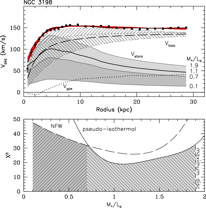
Figure 1: Example mass-decompositions for NGC 3198 for a factor of $\sim$20 range in $K$-band $\Upsilon_{\ast}$ (assumed constant with radius), constrained by the observed 21 cm (H I) rotation curve (points) and gas mass surface-density, adopting either a spherical pseudo-isothermal or NFW dark-matter halo profile. Stellar and halo mass-ranges (upper panel) are grey-scale coded (medium and light) for the break-point between halo models seen in the formal $\chi^{2}$ in the bottom panel. Total mass for the full range of $\Upsilon_{\ast}$ is shown (upper panel) in red (dark grey). All $\Upsilon_{\ast}$ values provide indistinguishably good fits to the observed rotation curve given the amplitude of non-axisymmetric motion (see text). The disk radial scale-length is 2.7 kpc. [COLOR IN ELECTRONIC EDITION ONLY]

As a specific example of the fundamental impasse with existing rotation curve decompositions, we illustrate in Figure 1 a traditional mass decomposition of NGC 3198 based on a tilted-ring derived H I rotation curve (Begeman 1989), and a photometrically-calibrated image that samples the stellar light distribution (here, a $K$ band image from 2MASS; Skrutskie et al. 2006), much the same as the original work by van Albada et al. (1985). We have carried out our own elliptical-aperture photometry on the 2MASS image. To focus discussion, we assume that the rotation curve is accurate in terms of sampling the projected major axis, and in being well-corrected for beam-smearing, inclination, and the possible presence of a warp; similarly, the photometric calibration also is assumed to be free of systematic error. In the case of NGC 3198 these are excellent assumptions, which is why the galaxy was chosen, but in general these are separate observational issues that cannot be ignored.

To make the decomposition with the data as posed, however, we must still assume the mass surface-density and thickness of the disk, and either a functional form and shape for the halo density profile (as we have done here), or adopt a non-parametric inversion solution. There are four ingredients in the disk-mass surface-density, typical of mass-decomposition methods: (i) We use the light profile to derive the stellar mass, assuming a value of $\Upsilon_{\ast}$ and its radial dependence. Here we assume $\Upsilon_{\ast}$ is constant with radius. The disk is given a typical oblateness (e.g., de Grijs & van der Kruit, 1997). (ii) We use 21-cm aperture-synthesis observations to determine the atomic gas mass, scaling the H I mass surface-density by a factor of 1.4 to account for Helium and metals. (iii) We estimate the molecular gas mass to be close to 20% of the H I mass, based on CO measurements from Braine et al. (1993). The spatial distribution is uncertain, although likely more concentrated than the H I. Because of the uncertainties in the conversion and distribution, we ignore the relatively minor molecular gas contribution. By this intentional oversight we can only underestimate the uncertainties in the stellar disk mass. (iv) We ignore the possible presence of disk dark-matter; it is implicitly subsumed into $\Upsilon_{\ast}$ or the inferred halo profile. Out of these four points, the outstanding ingredient is $\Upsilon_{\ast}$.

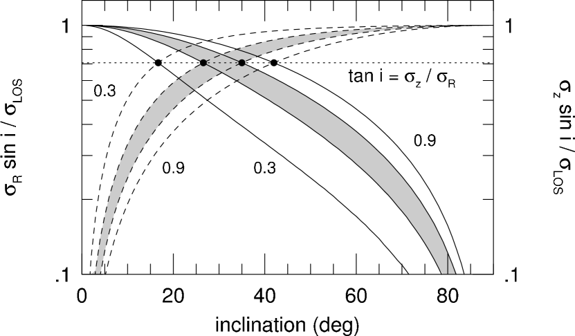
Figure 6: Projection of vertical and radial disk velocity-dispersion components ($\sigma_{z}$, solid lines; $\sigma_{R}$, dashed line) into the minor-axis line-of-sight as a function of inclination. Curves represent different assumed SVE shape parameterized by the ratio $\sigma_{z}/\sigma_{R}$. Ratios of 0.5 to 0.7, expected to be typical for galaxies in our survey (Paper II), are high-lighted in grey. Horizontal, dotted-line intersections with curves mark inclinations where radial and vertical projections are equal. Inclination values (i) at these intersections are related to the SVE axis ratio, as given in the figure.

Figure 1 shows that comparable fits to the observed rotation curve can be obtained for a factor of $\sim$20 in $\Upsilon_{\ast}$ (a factor of 4.5 in stellar-disk rotation velocity), while also providing a plausible range of dark-matter halo profiles. An acceptable fit is obtained even when setting $\Upsilon_{\ast}=0$ for the entire disk, as shown by van Albada et al. (1985). Even though $\Upsilon_{\ast}=0$ is not astrophysically plausible, this emphasizes their point that rotation curves can be used to set upper limits on $\Upsilon_{\ast}$, but not lower limits. While we have ignored the likely possibility that $\Upsilon_{\ast}$ varies with radius, relaxing our unphysical assumption (i) only improves the quality of the fits. A formal statistical interpretation of the $\chi^{2}$ distribution indicates $\Upsilon_{\ast}$ in the $K$ band is constrained to within factors of 1.8, 2.3, and 3.2 at the 65, 95, and 99% confidence levels (CL) for three degrees of freedom (i.e., $\Upsilon_{\ast}$, the halo central density, and characteristic radial scale). The same spirit of interpretation also leads to the conclusion that a pseudo-isothermal density profile is preferred at 95% CL over the NFW profile (Navarro, Frenk & White 1997), the latter motivated by simulations of structure-formation in a $\Lambda$CDM universe. However, these simplistic statistical interpretations are invalid because the errors are non-Gaussian and only describe estimated random uncertainties. Even this quiescent spiral galaxy has non-axisymmetric motions contributing to systematic variations in the measured tangential speed of order, or larger than, the estimated random errors (see Figure 6 in Begeman 1989). Until non-axisymmetric motions can be understood and modeled at the level of 5 km s^-1 on small physical scales associated with spiral arms and H II regions (the best work in the literature indicates this level of accuracy is not yet obtainable, e.g., Spekkens & Sellwood 2007), rotation-curve decomposition constraints on halo parameters and $\Upsilon_{\ast}$ are weak at best.

2.2 Uncertainties in $\Upsilon_{\ast}$ from SPS Models

Can such a large range in $\Upsilon_{\ast}$ values be accommodated given our knowledge of stellar evolution? Historically, we have expected variations are minimized at longer wavelengths where sensitivity to the presence of hot, massive stars is reduced. These stars are luminous, short-lived and span a wide range of stellar $M/L$. Based on this argument the $K$ band might appear ideal given the observational challenges of the thermal infrared and the presence of dust emission long-ward of 5 $\mu$m. However, Portinari et al. (2004) have advocated the $I$ band is best for estimating $\Upsilon_{\ast}$ because at 0.8$\mu$m one diminishes uncertainties due to late-phases of stellar evolution (e.g., the TP-AGB), while minimizing dependence on star-formation rates and dust. Bell & de Jong (2001) showed significant improvements could be made by considering simple correlations of $\Upsilon_{\ast}$ against color – both in the optical and near-infrared – for a wide range of SPS models. An exquisite refinement along both of these lines has been to take a multi-color approach to estimating $\Upsilon_{\ast}$, with a choice of band-passes (e.g., $g,i,H$) minimizing the impact of nebular emission, extinction, and TP-AGB (Zibetti et al. 2009). Assuming a single IMF, Zibetti et al. find a variance of 0.1 dex in $\Upsilon_{\ast}$ is typical over a wide range of multi-colors, but with up to 0.2 dex variance for blue colors typical of strongly star-forming galaxies. Unfortunately, they also find $\Upsilon_{\ast}$ up to 2.5 times smaller than earlier work (e.g., Bell et al. 2003). This requires some explanation. Consistent with the analysis of Bruzual (2007) and Conroy et al. (2009), they suggest the culprit is a change in the stellar evolutionary tracks for TP-AGB stars, which we now believe are longer-lived.

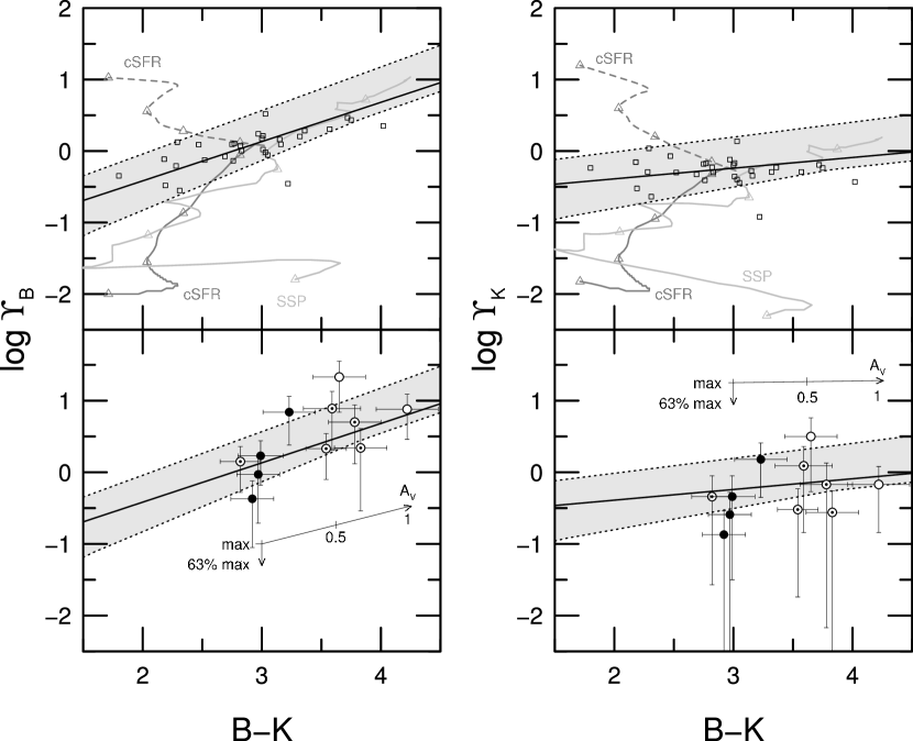
Figure 2: $B$- and $K$-band $\Upsilon$ versus $B-K$ color. Models: Solid black line and gray areas represent mean and extrema $\Upsilon_{\ast}$ for the full range of SPS models given in Bell & de Jong (2001); they scale their IMF such that no galaxies in the Verheijen (1997) sample are super-maximal (see text). Trends in $\Upsilon_{\ast}$ for SSP and cSFR models are plotted in the top panels as light and medium-gray lines punctuated by triangles marking age in time-steps from 10⁷ to 10¹⁰ years in equal dex intervals (Bruzual & Charlot 2003). For cSFR, $\Upsilon_{\rm dyn}^{\rm disk}$ is also calculated including gas mass in future star-formation up to 10¹⁰ years (dashed line). Observations: $\Upsilon_{\rm dyn}^{\rm disk}$ values and uncertainties for galaxy disks in the literature (see text). Open squares are estimates (Sanders & Verheijen 1998; top panel) based on rotation-curve decomposition assuming MOND for the same sample of galaxies later used by Bell & de Jong (2001). Circles (bottom panel) represent the Bottema (1993) sample, based on direct kinematic measurement marked here by inclination for face-on ($i<30^{\circ}$; filled), highly-inclined ($70^{\circ}<i<80^{\circ}$; dotted), and edge-on ($i>80^{\circ}$; open) systems. Reddening vectors are indicated, marked for 0.5 and 1 mag of visual extinction ($A_{V}$) in a foreground screen. Change in $\Upsilon_{\ast}$ from a so-called maximum disk (providing up to 85-90% of the observed galaxy rotation) to a disk which provides only 63% of this rotation is also indicated.

Figure 2 shows what one might expect in the $K$ band for a range of star-formation histories, formation epochs, metallicity ($0.008<Z<0.02$), extinction, enrichment models, and IMF, as adopted from the ground-breaking work of Bell & de Jong (2001). These use older SPS models, yet our illustration serves to show their full range of astrophysical parameters and several different SPS codes. All of these cases are astrophysically plausible, and produce colors reasonably matching those of today’s spirals. As they note, there is a correlation of $\Upsilon_{\ast,K}$ (the stellar mass-to-light ratio in the $K$ band) with color, here shown as the long-baseline optical-near-infrared $B-K$. While this band-pass choice may not be ideal for the reasons given above, it does serve as an excellent diagnostic of stellar-populations (e.g., Bershady 1995) and reddening.

For comparison, trends for a simple stellar population (SSP) and constant star-formation rate (cSFR) with Salpeter IMF (0.1 to 125 M_⊙) are also shown in the top panels of Figure 2 as a function of age from 10⁷ to 10¹⁰ years (Bruzual & Charlot 2003). For cSFR, $\Upsilon_{K}$ is also calculated including gas mass in future star-formation up to 10¹⁰ years, i.e., here $\Upsilon_{K}$ is the mass-to-light ratio of all the baryons in the disk, assuming a disk is formed with all its baryons from the beginning with no subsequent accretion or loss. From these trends we may surmise that stellar populations with characteristic ages below a few giga-years have rapid changes in $\Upsilon_{\ast,K}$ with age, and potentially extreme differences in $\Upsilon$ of the disk depending on gas content. This serves as a reminder that for predicting the baryonic mass of disks, we need a complete picture of the gas-accretion and re-processing history as well as a reliable zero-point for $\Upsilon_{\ast}$.

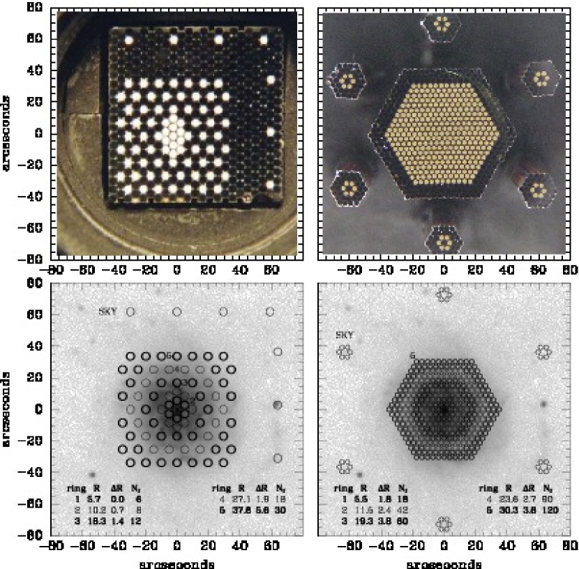
Figure 3: (Top row) Fiber integral-field units (IFU) developed for the DiskMass Survey, shown at the same angular scale: SparsePak (left, WIYN 3.5m telescope) and PPak (right, Calar Alto 3.5m telescope). Both IFUs subtend approximately 70 arcsec field in their core, sample with 4.7 and 2.7 arcsec diameter fibers, respectively, and reformat to feed grating-dispersed spectrographs in long-slit mode. Relevant spectrograph configurations, achieving $8000<\lambda/\delta\lambda<11000$ are given in Table 1. (Bottom row) SparsePak and PPak overlays on UGC 6918 $B$-band image from the KPNO 2.1m telescope, with examples of azimuthal rings of fibers identified. Inset tables specify mean sky-plane radius ($r$), half-range of radius ($\Delta r$) for fiber centers, and number of fibers per ring (N_f).

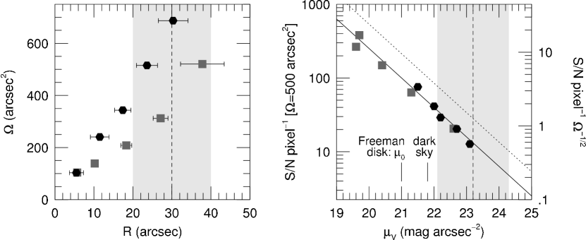
Figure 4: (Left panel) Solid-angle versus radius in five radial bins for SparsePak (grey squares) and PPak (black hexagons). Horizontal bars represent radial range in fiber centers for each bin. (Right panel) S/N per pixel as a function of $V$-band surface-brightness for stellar absorption-line spectroscopy in the Mg IB region in a ring subtending 500 arcsec². Rightmost vertical scale gives equivalent S/N per arcsec². Data for UGC 6918 (SparsePak) and UGC 1635 (PPak) are scaled to this $\Omega$ and typical total integration-times with these instruments (12 and 8 hr, respectively). Diagonal lines are the predicted, detector-limited performance for the typical (solid) and longest (dotted) total integration times. In both panels grey shaded regions in both panels mark the distribution of apparent size and surface-brightness at $2.25h_{R}$ encompassing 90% of the galaxies in the DiskMass sample; vertical dashed lines represent median values.

Focusing here on the $\Upsilon_{\ast}$ zero-point, Bell & de Jong (2001) state there is a factor of 2 range in $\Upsilon_{\ast,K}$ in today’s disks given a ‘plausible range’ in model parameters. However their Figures 1, 3, and 4 clearly show a wider span over their full parameter inventory. Based on their compilation we find an 0.5 dex range (a factor of 3) in $\Upsilon_{\ast,K}$ for a given $B-K$ at the extrema; and 1.2 dex (a factor of 15) range over $2<B-K<4$, typical of spiral galaxies (e.g., Bershady 1995), again at the extrema. To further complicate matters, the later work of Bell et al. (2003) shows significant differences compared to Bell & de Jong (2001) both in trend, zero-point and scatter in $\Upsilon_{\ast,K}$ when calculated using different SPS models, different ranges of age and metallicity, but the same so-called “diet” Salpeter IMF. Certainly differences in stellar-population mean age is a critical factor, as seen in our Figure 2. Albeit our estimates include their full suite of models it is reasonable to ask: What, a priori, defines a plausible range or distribution of models given our extant knowledge of galaxy formation and evolution and its range of variation? This is a particularly hard question to answer because of the degeneracy in galaxy colors for a wide range of model parameters.

Portinari et al. (2004) present arguably the most sophisticated analysis of SPS models applied to estimating $\Upsilon_{\ast}$ from galaxy colors, including a self-consistent treatment of chemical enrichment. They are able to break out the different physical effects driving variations in the $\Upsilon_{\ast}$ model predictions, finding a factor of 2.5 range in $\Upsilon_{\ast}$ for variations in star-formation histories that yield comparable colors, but only about 25-50% variation in $\Upsilon_{\ast}$ from metallicity effects due to different chemical evolution histories. However, they find an additional factor of 2 uncertainty in the $\Upsilon_{\ast}$ zero-point from a variety of plausible IMF. To all of this, recall there is an additional factor of 2 to 2.5 uncertainty in $\Upsilon_{\ast}$ in the near-infrared due to uncertainties in the lifetime of TP-AGB stars. Combining these effects as random processes yields a factor of $\sim$4 uncertainty in predicting $\Upsilon_{\ast}$ from photometry, and as much as a factor of 10 to 20 uncertainty if systematic. Consequently the path to accurate and precise mass-decompositions and study of dark-matter halo profiles is blocked based on a purely photometric approach to disk-mass estimation.

In this context it is worth noting that Bell & De Jong (2001), and hence Bell et al. (2003), calibrate the $\Upsilon_{\ast}$ zero-point by tuning the low-mass end of their “diet” Salpeter IMF to yield disks in the Verheijen (2001) rotation-curve sample that are close to maximal. Not only is the tuned, critical mass-range of the IMF unconstrained for galaxies outside of the Milky Way, but Conroy et al. (2009) point out even the Milky Way’s IMF determinations have considerable uncertainty between 0.8-2 M_⊙. In this range, the estimation requires uncertain stellar evolution corrections for solar-neighborhood field stars. This now brings us back full circle to the disk-halo degeneracy and the unproven, maximum-disk hypothesis.

Finally, we would like to know what level of precision and accuracy on $\Upsilon_{\ast}$ is needed to infer meaningful information about the dark matter halo. One basic fact to establish is whether a dark halo is needed at all in the inner regions of spiral galaxies. A closely related question is whether we can differentiate between a maximum disk and modified gravity based on measurements in these inner regions. Since maximum disks contribute 85-90% of the rotation at two disk scale-lengths, it is therefore not surprising that estimates of the required $\Upsilon_{\ast}$ with modified Newtonian gravity (MOND, e.g., Sanders & Verheijen 1998, McGaugh 2005) nearly agree with SPS models calibrated in this way for normal surface-brightness disks, particularly given the scatter due to other SPS parameters (see top panels of Figure 2). To falsify MOND via this line of argument, and simultaneously to make serious headway into understanding the shape of dark-matter halo cores, requires a level of precision on the mass surface-density of the disk, and hence $\Upsilon_{\ast}$, of 30% or better, i.e., 10 to 15% in rotation velocity.

2.3 Breaking the Disk-Halo Degeneracy

The path around the decomposition impasse is to make direct, dynamical estimates of the mass of galaxy disks. One direct and absolute measurement of the dynamical mass-to-light ratio of a galaxy disk ($\Upsilon_{\rm dyn}^{\rm disk}$) can be derived from the vertical component, $\sigma_{z}$, of the disk stellar velocity dispersion (van der Kruit & Searle 1981; Bahcall & Casertano 1984) and the vertical thickness of the disk. Other promising approaches include lensing (e.g., Maller et al. 2000), and using hydrodynamical modeling of non-axisymmetric gas-flows around bars (Weiner, Sellwood & Williams 2001) or spiral arms (Kranz, Slyz & Rix 2001). Here we focus on collisionless tracers of the disk potential. For a locally isothermal disk, where the vertical density distribution decreases with height $z$ above the mid-plan as ${\rm sech}^{2}(z/z_{0})$, $\sigma_{z}=\sqrt{\pi\,{\rm G}\,\Upsilon_{\rm dyn}^{\rm disk}\,I\,z_{0}}$, with $I$ the surface-intensity (flux per unit area), and $z_{0}$ the disk vertical scale parameter (van der Kruit & Searle 1981). Disk-mass surface-density is then

$$\Sigma_{\rm dyn}=\sigma_{z}^{2}/\pi{\rm G}z_{0}.$$ (1)

Other functional forms for the vertical distribution modify these relations by a small change in scale factor. The observational conundrum is how to determine a parameter like $z_{0}$, best seen at edge-on projections, and $\sigma_{z}$, best seen in face-on projections, at the same time. We argue (§4.1 and Paper II) a face-on approach favoring $\sigma_{z}$ is preferred for a number of reasons, but principally because little is known empirically about the shape of disk stellar velocity ellipsoids (SVE), while disk scale-heights are statistically well-determined from studies of edge-on galaxies (e.g., de Grijs & van der Kruit 1996, Kregel et al. 2002). Thus, $\sigma_{z}$ provides a direct, kinematic estimate of $\Sigma_{\rm dyn}$ and $\Upsilon_{\rm dyn}^{\rm disk}$ to break the disk-halo degeneracy. This, in turn allows us to unambiguously determine the density profiles of dark matter halos. With additional analysis of the disk gas content and extinction, we may also constrain $\Upsilon_{\ast}^{\rm disk}$ and the IMF over a broad range of global galaxy properties local densities and environments within each galaxy.

This kinematic approach to measuring disk mass has been attempted before with long-slit spectroscopy, pioneered by van der Kruit & Freeman (1984, 1986) on several face-on and inclined systems. This work was the starting point and inspiration for the first survey carried out by Bottema (1997, and references therein). However, these observations barely reached 1.5 disk scale-lengths and required broad radial binning. Further, the face-on samples suffered from significant uncertainties in the inclination, and hence total-mass estimates, while measurements of more inclined systems required large and uncertain corrections to the observed line-of-sight velocity dispersions ($\sigma_{\rm LOS}$) for the tangential ($\sigma_{\theta}$) and radial ($\sigma_{R}$) components of the SVE.

To illustrate the limitations of extant data, the spread of $B$- and $K$-band $\Upsilon_{\rm dyn}^{\rm disk}$ in Bottema’s (1993) sample is illustrated in the bottom panels of Figure 2. We use his formula (equation 8), which requires a central disk surface-brightness ($\mu_{0}$), a central vertical velocity dispersion ($\sigma_{z,0}$), and a disk scale-height ($z_{0}$). The formula and/or the $\sigma_{z,0}$ estimates assume (i) the SVE shape is constant with radius and the same for all galaxies; (ii) the disk scale-height and $\Upsilon_{\rm dyn}^{\rm disk}$ are constant with radius; and (iii) the disk is purely exponential. The validity of these assumptions are all debatable. We take velocity dispersions, scale-lengths, and $B$-band disk surface-brightness primarily from Bottema (1993) and earlier papers in that series, with some supplemental surface-brightness and scale-length measurements in the $B$ and $V$ bands compiled from the literature (van der Kruit & Freeman 1986; Baggett et al. 1998; McGaugh 2005). Scale-heights are estimated from the observed scale-lengths using our calibration (Paper II). $B-K$ colors are based on values from NASA/IPAC Extragalactic Database (NED), corrected to total magnitudes as described in Appendix A, corrected for Galactic extinction (but not internal extinction), and then transformed to disk colors based on bulge-to-disk ratios in the $B$ and $K$ bands measured as a function of type by Graham (2001). Errors are estimated based on the quoted observational uncertainties, differences between repeat measurements, and, in the case of $\Upsilon_{{\rm dyn},K}^{\rm disk}$ and $B-K$, the dispersion in bulge-to-disk ratios for galaxies of a given type.

Trends in Figure 2 of $B$-band $\Upsilon_{\rm dyn}^{\rm disk}$ with $B-K$ color correlate with inclination; this is likely an internal extinction effect. Hence the range of intrinsic $B-K$ color is small (likely less than 1 mag). Given Bottema’s small sample size and large errors, scatter in $\Upsilon_{\rm dyn}^{\rm disk}$ – even in the $K$ band over this color range – is too large to make reliable statements about disk maximality, trends with color, or the viability of MOND. Limitations notwithstanding, these earlier studies pointed the way forward (e.g., Herrmann & Ciardullo 2009). Indeed the program we describe here is very much a modern version of what Bahcall & Casertano (1984) outlined many years ago.

3 THE DISK-MASS SURVEY

To surmount past limitations while taking advantage of the benefits of a direct, kinematic measurement of the mass of spiral disks, we have built instruments, designed an analysis protocol, constructed an observational strategy, and carried out a survey targeting nearly face-on systems. We refer to this as the DiskMass Survey. The range of disk inclinations was chosen (§4.1) to balance uncertainties in de-projection of both the total mass (via rotation curves) and disk mass (via vertical velocity dispersions). This inclination choice and the spectroscopic instrumentation built to sample kinematics in such nearly face-on systems are the survey’s hallmarks.

The DMS scope is to measure the mass surface-density in regular, moderate-to-late type disks spanning a range in color, luminosity, size, and surface-brightness that characterize these types of ‘normal’ disk systems today. The impetus to define such a sample is several-fold. First, such a sample should include galaxies like the Milky Way, for which we have unique (albeit limited) measurements of the disk mass within the solar neighborhood. Second, our definition is similar to typical TF samples that have served both as cosmological probes and key tests of semi-analytic models of structure formation. Third, for such a sample, bulge contributions to the stellar kinematics are minimal outside of the inner disk scale-length. With these considerations in mind, the range of physical properties sampled are significant (e.g., factors of 10 to 100 in size and luminosity). The required sample size (§4.2) then follows from our intent to sample the cosmic variance in key physical parameters (e.g., disk-to-total mass, SVE shape, disk oblateness), as well as draw out the principal correlations these parameters have with other physical properties of spiral galaxies (e.g., luminosity, surface-brightness, integrated stellar populations). The details of the sample are described in §5.

The DMS experimental paradigm centers around optical bi-dimensional spectroscopy obtained with custom-built integral-field units (IFUs). These instruments were used to measure stellar and ionized gas kinematics at multiple wavelengths from 500 to 900 nm, as described in §4.2, covering the key spectral diagnostics of [O III]$\lambda$5007 and H$\alpha$ in emission, and Mg IB and Ca II near-infrared triplet (hereafter Ca II-triplet) in stellar absorption. From these observations we are able to derive kinematic inclinations, total mass, star-formation rates and SVEs on a spatially resolved scale for each galaxy. The broad spectral coverage at high dispersion was essential for providing several important diagnostics and checks on systematics concerning our kinematic signal due to internal extinction and variations in stellar populations across the face of individual galaxies.

The two IFUs built for this survey were optimized, capitalizing on the potential of two existing spectrographs, for the measurement of two-dimensional velocity functions (e.g., centroids, dispersions, and higher moments) of the stars and gas in spiral disks. The salient technical hurdle was to achieve photon-limited, medium-resolution spectroscopy at surface-brightness levels at and below the sky foreground continuum. SparsePak (Bershady et al. 2004, 2005) and PPak (Verheijen et al. 2004, Kelz et al. 2006) are large-fiber IFUs on 3.5m telescopes (WIYN and Calar Alto, respectively) with fields-of-view of slightly over 1 arcminute. Both IFUs, illustrated in Figure 3, feed conventional long-slit, grating-dispersed spectrographs (the Bench Spectrograph and PMAS, respectively) configurable over a wide range of wavelengths and spectral resolutions. The configurations relevant to the DMS are the high-dispersion modes for Mg IB (PPak and SparsePak), H$\alpha$ (SparsePak), and Ca II-triplet (SparsePak) as summarized in Table 1. Photon shot-noise is comparable to read-noise in these configurations (Bershady et al. 2005) for dark, sky-limited conditions. Since these IFUs are among the largest-grasp systems in existence (Bershady et al. 2004), and grasp is conserved, their performance serves as a cautionary note for instruments striving for higher angular or spectral resolution, even on larger telescopes.

Near the detector-limited regime, signal-to-noise (S/N) $\propto\sqrt{d\Omega\ \Omega}$, where $d\Omega$ and $\Omega$ are the specific solid angle associated with each fiber and the total solid angle of the IFU array, respectively. In all noise regimes, (S/N) $\propto\ \sqrt{\Omega}$ for extended sources. The total solid angle of SparsePak and PPak is 1280 and 1891 arcsec², respectively. The major advantage of integral-field spectroscopy (IFS) over long-slit observations is the ability to group together fibers (i.e., coadded spatial resolution elements) in radial bins. An example, typical of what is used in our survey, is shown in Figure 3. The solid angles covered as a function of radius for each of these 5 radial bins is plotted in Figure 4 for both IFUs. In the outer-most rings, these instruments sample 500 to 700 arcsec², i.e., a 6th of an arcmin².

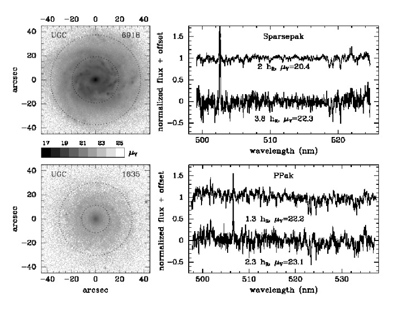
Figure 5: Survey spectroscopic dynamic range in surface-brightness, shown with KPNO 2.1m $V$-band images (60 sec exposures) and spectra in the Mg IB region for UGC 6918 (top; 2.25 hours SparsePak total integration in 3 exposures) and UGC 1635 (bottom; 6 hours PPak total integration in 6 exposures). These galaxies span the surface-brightness range of our survey. Image grey-scale is logarithmic, calibrated in magnitudes. Radial bins, labeled on spectra and marked on images, consist of 12 and 18 fibers (subtending 208 and 382 arcsec² solid-angle) for SparsePak, and 60 and 120 fibers (subtending 344 and 687 arcsec² solid-angle) for PPak. Spectra are plotted in the observed frame of each instrument in normalized flux units. Mean S/N per pixel is 42 and 10.5 for SparsePak spectra of UGC 6918 at 2 and 3.8 h_R, and 21 and 13 for PPak spectra of UGC 1635 at 1.3 and 2.3 h_R.

With this formidable grasp, we are able to achieve a S/N of 12 per pixel, or S/N $\sim 22$ per resolution element at V-band surface-brightness of 23.2 mag arscec^-2 for spectral resolutions (FWHM) of $\lambda/\delta\lambda\sim$ 8,000 and 11,000 (velocity dispersions of $\sigma\sim$ 16 and 11 km s^-1) in 8 and 12 hours, respectively, for PPak and SparsePak. These are typical exposures for galaxies in our survey. This surface brightness is equivalent to that of an exponential disk at 2.25 scale-lengths, given the median central surface brightness of our sample is 21.4 mag arcsec^-2 in the $B$ band. This is roughly 0.25 mag brighter than a so-called Freeman disk (Freeman 1970). Figure 4 also shows the delivered spectroscopic S/N in the outermost ring as a function of surface-brightness in our typical, and our deepest, exposures. We obtain S/N = 10 per pixel or better at the faintest limits of our survey, which is ample for our purposes, as we quantify in Paper II. Figure 5 presents the coadded spectra in the outermost radial bins for two galaxies near the extrema of the surface-brightness range of our survey: UGC 6918 (a short exposure with SparsePak), and UGC 1635 (a moderate exposure with PPak). In addition to the strong nebular line of [O III]$\lambda$5007 and absorption line of the Mg IB triplet, the weak nebular doublet [N I]$\lambda\lambda$5198,5200 and a plethora of weak Fe, Ti, and Cr absorption lines are clearly distinguishable. We find S/N scales as expected with exposure and coaddition.

The DMS, as a study of nearby galaxies, is distinguished by its emphasis on (i) observations of spatially-resolved kinematics of both gas (ionized and neutral) and stars; (ii) the direct measurement of dynamical mass surface-density and $\Upsilon_{\rm dyn}^{\rm disk}$; and (iii) focus on intermediate-to-late-type disk systems. The galaxies studied were chosen carefully to match the survey spectroscopic instruments for efficient observation. As such, the galaxy sample is more distant than, say, the typical galaxy in the SINGS sample (Kennicutt et al. 2003), and more narrowly focused on normal spiral galaxies. Even with our spectroscopic focus, photometric observations are a necessity both to place these observations in a broader context, more completely characterize the sample, and to properly define and interpret $\Upsilon$ measurements in terms of stellar populations, star-formation, and galaxy type. Accordingly, the survey as a whole was fleshed out around our spectroscopic observations to include ground- and space-based photometric data in the optical, near-, and mid-infrared. Wherever possible we take advantage of existing photometric observations in the public domain, supplementing with new observations as necessary to increase depth or spectral coverage. Substantial investment has been made with new observations using the Spitzer Space Telescope (hereafter, Spitzer) as well as the KPNO 2.1m telescope. In addition, new, 21 cm, aperture-synthesis observations were also undertaken with the VLA, GMRT, and Westerbork facilities to radially extend our gas-kinematic measurements and measure H I mass.

Several observational precursors were motivational in the design and execution of the DMS. The TF study of Verheijen (1997, 2001) provided the foundation for understanding the extent of possible variations in the correlation of light to mass in spiral galaxies; the importance of the near-infrared in this regard; and the subtleties of defining rotation curve amplitudes in this analysis. Ionized-gas kinematic studies of face-on galaxies (Andersen 2001; Andersen et al. 2001) were critical in understanding the power of IFS, and for developing the techniques for deriving kinematic inclinations in the nearly face-on regime. Finally, a pilot survey (Bershady, Verheijen & Andersen 2002; Verheijen, Bershady & Andersen 2003) carried out during SparsePak commissioning established the basic capabilities of the survey IFUs.

4 SURVEY STRATEGY

4.1 The Nearly Face-On Approach

Because the two primary observables contributing to the estimation of $\Sigma_{\rm dyn}$, namely $\sigma_{z}$ and $z_{0}$, have orthogonal projections to the observer’s line-of-sight, the choice of galaxy inclination is paramount in optimizing the error budget. Intermediate inclinations proffer access to both $\sigma_{z}$ and $z_{0}$, but in practice the task is difficult: $\sigma_{z}$ is quickly overwhelmed by the other SVE components if, as expected, $\sigma_{z}$ is the smallest component; non-axisymmetric photometric features in disks associated with spiral structure (e.g., dust, star-formation) preclude a simple estimation of disk thickness at all but nearly edge-on orientations. Consequently, compelling survey strategies either focus on edge-on galaxies, where the vertical scale-height can be directly observed, or on nearly face-on galaxies where $\sigma_{\rm LOS}$ is dominated by the $\sigma_{z}$ component. The projection of $\sigma_{z}$ into the line-of-sight along a galaxy’s kinematic minor axis is shown in Figure 6 as a function of inclination and SVE shape. In the edge-on case $\sigma_{\rm LOS}$ contains nothing of $\sigma_{z}$, and hence one must rely on knowledge of the SVE to extract this vertical component. Conversely, in the face-on case one must rely on knowledge of the typical vertical scale-height of the kinematically-probed stars, or a re-scaling of the radial scale-length based on an adopted disk oblateness.

The goal of our survey strategy is to be limited by the uncertainties in the disk vertical scale-height of galaxies, specifically the dispersion in the relation between $z_{0}$ and observables that do not require edge-on orientation (Paper II). In other words, we opt for the “face-on disk” approach. Our rational is several-fold. Foremost is the fact that $\Sigma_{\rm dyn}$ depends quadratically on $\sigma_{z}$, but only linearly on $z_{0}$. Furthermore, we know far less about the shape of the disk SVE than about disk photometric oblateness. As we quantify in Paper II, our ability to estimate disk oblateness in face-on galaxies is 2-4 times better than our ability to estimate the SVE in edge-on systems. This translates into a 4 to 16 times increase in precision for measuring disk-mass in the face-on regime.

On top of these primary considerations, given the complications of projection and extinction in edge-on galaxies – for both kinematics and photometrics – clearly the face-on approach is desirable in terms of minimizing systematics. Since surface-brightness falls off exponentially in disks, the past observational challenge has been to gather enough light in the outer regions of disks to make a sufficiently precise kinematic measurement. Edge-on galaxies conveniently project the disk light into a geometry suitable for a long-slit spectrograph. However, with our development of appropriately sized IFUs, we can fully sample face-on disks, and optimally average in azimuth and radius as our detailed analysis requires. The coupling of a nearly face-on approach with IFS means that systematics can be minimized without enlarging our random errors – again, the hallmark of our approach. Inclinations close to 30 degrees are optimal for determining the disk-mass surface-density simultaneously with the total galaxy mass (Paper II), and conveniently are also optimal for measuring the SVE (Westfall 2009). As shown in Figure 6, this is where we expect the radial and vertical components of the SVE to equally project into the line-of-sight.

4.2 Scope and Protocol

Our aim is to sample the disk dynamical and stellar mass-to-light ratios ($\Upsilon_{\rm dyn}^{\rm disk}$ and $\Upsilon_{\ast}^{\rm disk}$) of intermediate-to-late type spiral galaxies spanning a range in luminosity, surface-brightness, and color, but with only a modest range in other morphological attributes. For this sample, we also aim to know the gas content and star-formation rate on a spatially resolved scale commensurate with the measurements of disk $\Upsilon_{\rm dyn}^{\rm disk}$. With 3 bins in each parameter (luminosity, surface-brightness and color), a sample of $\sim$40 galaxies is needed to have a sufficient number of galaxies in each bin. This is not simply to diminish our random errors, but also to limit our systematic errors, as discussed in Paper II, and to understand the range of astrophysical variance in $\Upsilon_{\rm dyn}^{\rm disk}$ and $\Upsilon_{\ast}$. These aims set the basic scope of our survey.

4.2.1 Down-Selecting

The spectroscopic requirements of the survey are demanding, with the stellar absorption-line observations by far the most taxing. To make the survey data acquisition tractable, we designed a two-phase protocol following a down-selecting scheme. The protocol focuses resources on a modest sub-sample of galaxies, yet provides a large enough parent sample to place our study into the context of disk-galaxy properties and scaling relations. The selection criteria and sample details for each of these phases are given in §5.

The initial survey phase, Phase-A, is based on a purely photometric selection of a large number of targets that suit our observational and scientific criteria. After detailed inspection, roughly 14% of this parent sample was deemed suitable for spectroscopic investigation of their ionized-gas kinematics. H$\alpha$ velocity fields for 63% of these sources were successfully obtained (about 9% of the parent sample defined in §5.1). Ground-based optical and near-infrared observations targeted this subset. Observations in this phase had the immediate purpose of enabling us to estimate inclination, total mass, and mass-luminosity scaling properties; the additional purpose of establishing their kinematic regularity for Phase-B selection; and the final purpose of estimating star-formation rates and diagnostics parameters of the inter-stellar medium(ISM) such as line-widths and ratios of the ionized gas.

In the second phase, Phase-B, we further down-selected $\sim$32% of the spectroscopically-observed Phase-A sample for intensive further study, including spectroscopic observations of their stellar kinematics, aperture-synthesis observations of their H I distribution, and Spitzer observations of their mid-IR flux distributions. This core sample amounts to $\sim$20% of the initial Phase-A sample, and only 3% of the parent sample.

4.3 Spectroscopic Coverage

Spectral regions were chosen to characterize neutral- and ionized-gas content and kinematics via emission, and stellar kinematics via absorption-line observations.

4.3.1 Gas kinematics

For the Phase-A sample, the H$\alpha$ region was selected because of the strength of the Balmer line; the ability to sample other, strong nebular lines ([N II]$\lambda\lambda$6548,6583 and
[SII]$\lambda\lambda$6716,6730) even in the small spectral range sampled at medium resolution; the utility of H$\alpha$ as a star-formation-rate (SFR) indicator; and finally because of the relative efficiency of obtaining velocity fields using SparsePak on the WIYN Bench Spectrograph. Spectroscopic observations are described in §6.1.

For the Phase B sample, spatially-resolved H I observations were a critical augmentation because the observable H I gas disks typically extend well beyond the field-of-view of the SparsePak IFU with which the H$\alpha$ velocity fields have been mapped and from which the inner rotation curves have been determined. From the more extended H I velocity fields, the rotation curve can be measured well into the outskirts of the galaxies where the dynamics are dominated by the dark matter halo. This allows us to properly measure the radial density profiles of the dark matter halos from an unambiguous rotation curve decomposition. Extended H I velocity fields and rotation curves are also required for detailed Tully-Fisher studies. Aperture-synthesis observations at 21 cm with the VLA, WSRT and GMRT are described in §6.1.2.

Our 21 cm observations also serve to constrain the gas-mass budget. By measuring the H I column-density distribution in the disk, we determine the total (H+He) gas surface-density. This is essential for properly calibrating the stellar mass-to-light ratio of the disk, $\Upsilon_{\ast}^{\rm disk}$, especially in the outer regions. The neutral gas-density is also of interest in relation to SFR indicators (e.g., H$\alpha$, 24 $\mu$m flux, etc.) to study star-formation thresholds and gas-consumption time-scales, and hence better link observed stellar populations with their star-formation histories and potentials.

4.3.2 Stellar kinematics

Several considerations led to the definition of the stellar-kinematics observations. Primary was to obtain a measure of the kinematics of the old stars that are dynamically relaxed, and therefore well-sample the disk potential, and are representative of the stellar population dominating the vertical light distribution in red and near-infrared light of edge-on samples. Secondary was to sample, if at all possible, both the stellar and ionized-gas kinematics simultaneously, in one spectroscopic-instrumental setting. Overall, the instrumental configurations were required to deliver spectral resolutions above $\lambda/\delta\lambda=8500$ ($\sigma<15$ km s^-1) and have reasonable efficiency.

Our primary consideration for the stellar-kinematic measures is critical because it is well known that the scale-height and velocity dispersion of stars in the Milky Way are correlated with their spectral type, and presumably their mean age. The physical picture is that stars, born in the disk mid-plane, slowly diffuse and dynamically relax with time. This picture should apply generally to other disk systems, and hence our measurement scheme must be sensitive to, or avoid systematics in disk-mass measurements due to this physical effect. This effect would include, for example, the impact of an older thick-disk component on both the effective (light-weighted) vertical scale-height and $\sigma_{\rm LOS}$.

Historically, the spectral regions of interest for stellar-kinematic work has stemmed from a focus on early-type galaxy observations. Since such galaxies do not suffer from hot-star contamination, the strong H&K lines near 400 nm, in combination with the ubiquitous and intrinsically narrow Fe lines in the blue have been a favored target well matched to optical spectrograph performance and low sky foregrounds. In galaxies with composite stellar populations, as in our survey, the picture is necessarily more complicated. The 400-nm region is too blue to have sufficient sensitivity to the old stellar population in our survey galaxies.

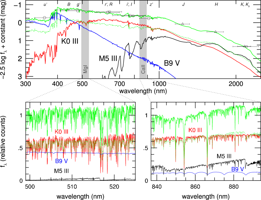
Figure 7: Three-star spectral-synthesis for UGC 6918, with integrated colors typical of galaxies in the DMS, at low-resolution (top panel) and high-resolution (bottom panels). Low-resolution spectra are from the compilation of Bruzual & Charlot (1993). High-resolution spectra are from our own echelle stellar-template library observed with SparsePak, and show the spectral regions used to measure $\sigma_{\rm LOS}$ in the DMS. Constraints on the spectral mix, described in the text, are based on broad-band photometry shown here as squares [$BVIK$ magnitudes from Verheijen (1997)], circles ($u^{\prime}g^{\prime}r^{\prime}i^{\prime}z^{\prime}$ magnitudes based on our own photometric measurements on SDSS images), and triangles ($JHK_{\rm s}$ measurements from 2MASS corrected as described in Appendix A). Individual star spectra are labeled (blue, red, black for B9 V, K0 III, and M5 III, respectively). In the Mg IB-region and Ca II-region the flux ratios B9:K0:M5 are 0.42:0.56:0.02 and 0.12:0.65:0.23, respectively. Green solid curves show the combined spectrum using this mix. Green dotted curves are the combined spectrum renormalized to the dominant stellar spectrum in the Mg IB region (top and bottom left panels) and Ca II region (bottom right panel), drawn to indicate the difference with a one-star template. [COLOR]

To illustrate the issues of sampling the old stellar disk population, Figure 7 shows a simple, 3-star spectral decomposition of intermediate-type spiral galaxy with colors typical of our sample. The decomposition is motivated by the earlier work of Aaronson (1978) and Bershady (1995), and in fact uses the specific stars Bershady found most-frequently provided best fits to galaxy colors of this intermediate (spectral) type. While the fit is not unique, it provides an excellent match to the observed optical to near-infrared broad-band colors, and is representative of the types of stars which dominate the integrated light at different wavelengths. The three stars (B9 V, K0 III, and M5 III) represent young, old, and intermediate-age stellar populations, respectively. Ideally it is the K-giant population we would like to sample. Below 500 nm, hot young stars dominate; above 500 nm K-giants dominate, but at near-infrared wavelengths there is an increasing contribution from intermediate-age M-giants.

Two facts provide nuance to this picture. Hot stars, outside of the Hydrogen and Helium lines, have weak spectral features, and so their contribution to the kinematic signal is effectively to diminish the amplitude of the old-star signal, but not to modulate significantly the velocity structure. However, late-A and F-stars, also characteristic of intermediate-age populations do contribute some signal in metal absorption lines (see §6.2.2); these stars, if in sufficient abundance, may modulate the kinematic signal in the visible. Consequently, the blue-visible region may also have significant contribution from intermediate-age stars. These considerations drive us to work in the 500-1000 nm region, i.e., farther in the red, but not too far into the near-infrared to become dominated by potential intermediate-age TP-AGB stars or red super-giants in vigorously star-forming regions.

In the 500-1000 nm range, popular regions for stellar kinematic study have included the Mg IB-triplet region near 513 nm and the Ca II-triplet near 860 nm, with the latter enabled by red-sensitive CCDs. Studies using the Ca II-triplet region have the advantage that a single gravity-insensitive ion dominates the cross-correlation signal. Therefore one would expect it simpler to match the temperature and metallicity between stellar templates and the target galaxy, thereby minimizing systematic error in the derived kinematics. In contrast, Barth, Ho & Sargent (2002) point out the potential difficulties in the Mg IB-triplet region due to a combination of ions whose strength vary with both temperature, metalicity and relative abundance. We find (Paper II) that the dependence of the derived $\sigma_{\rm LOS}$ on template temperature is comparable in amplitude, although different in trend in these two regons. One of the clear disadvantages of the Ca II-triplet region for measurement of velocity dispersions in dynamically cold systems is the great strength of the lines, which therefore are intrinsically broad. Bershady et al. (2005) measured intrinsic widths of the Ca II-triplet between 25-35 km s^-1 ($\sigma$) in cool stars in the context of cross-correlation measurements with SparsePak, directly relevant to the study at hand. They found the Mg IB triplet (513 nm) has similar intrinsic widths to the Ca II-triplet, but is surrounded by weak iron lines with intrinsic widths of only 7-8 km s^-1. For disk systems, where dynamical widths are expected to be of order 10’s of km s^-1, narrow (and therefore weak) lines are essential. This points to a final desideratum, namely we would like a region where there are some strong lines that can be used for velocity centroiding (e.g., spectral stacking, §5.2), but many weak lines so there is significant signal from intrinsically narrow features (in the absence of velocity broadening from the galactic potential).

The Mg IB region is particularly good in this regard, and offers three other advantages relative to the Ca II-triplet and other regions: (i) the presence of [O III]$\lambda\lambda$4959,5007 doublet within a spectral window small enough to contain key absorption-line features measurable at high-dispersion; (ii) low sky-foregrounds, and in particular the absence of strong sky line-emission; and (iii) relatively good instrument performance. (A comparison of the WIYN Bench Spectrograph performance in Mg IB and Ca II-triplet regions is given in Bershady et al. 2005; in the case of PMAS, no grating was available with adequate resolution in the Ca II-triplet region). While an intermediate-wavelength region, such as 600 nm might be ideal from a stellar-population perspective, and weak lines do exist there, no strong absorption or nebular line-emission is present. The H$\alpha$ region, just slightly to the red, is devoid of sufficient absorption-line signal. Our primary region for measuring stellar-absorption was then adopted to be the Mg IB region. However, multiple wavelengths permit independent determinations of our primary observable, the SVE, thereby providing a critical cross-check on systematics due to cross-correlation template-mismatch or astrophysical variance in scale-heights and velocity dispersion with stellar type. Accordingly, we observed with SparsePak a subset of galaxies in the Ca II-triplet region as a cross-check on our Mg IB observations.

4.3.3 Spectral Library

One critical issue for estimating $\sigma_{\rm LOS}$ accurately is determining suitable templates for deriving the broadening function. The so-called “template mismatch” problem arises when the derived broadening function is systematically in error due to the unsuitable match between stellar template and galaxy spectrum. Template-mismatch is thought to be relatively minor for early-type galaxies observed in the blue-visible (400-500 nm) portion of the spectrum and for any galaxy observed in the Ca II region. For the former, the approximation of early-type galaxies to simple stellar populations means a single stellar template best representing the tip of the red giant branch (e.g., G8 III to K1 III) is likely a good first-approximation. For the latter, the intrinsic width of the Ca II lines which dominate the kinematic signal in this spectral region are weakly dependent on spectral type.

Because the DMS focuses on intermediate-type spirals with on-going star-formation, these simplifying assumptions are not valid. Not only are the DMS spirals clearly composite (young+old) stellar populations, but given the uncertainties in the TP-AGB life-time, contributions from very cool stars may also be significant, particularly in the Ca II region. The impact of this complexity is illustrated in Figure 7. In light of the potential for independent thin disk / thick disk kinematics that correlate with stellar population age and metallicity, an application of the simultaneous multi-component kinematic study of de Bryne et al. (2004) to spiral disks may be necessary.

For these reasons, a large template library that spans temperature and metallicity is important for our program. When we began the survey, there were no population synthesis models available with spectral resolution comparable to our data. While this has begun to change (e.g., Le Borgne et al. 2004), it was observationally inexpensive to gather our own library (§6.2.2). These observations allow us to synthesize stellar populations while at the same time minimizing systematic errors due to instrumental signatures present or absent in model spectra. This is an important issue that we return to in Paper II.

4.4 Photometric Coverage

4.4.1 Optical–near-infrared wavelengths

Existing photometric data for all galaxies in the DMS consist of optical DSS blue and red images, as well as 2MASS (Skrutskie et al. 2006) near-infrared images and photometry, along with on-line compilations, e.g., NED, from which we extract $B$-band photometry from RC3 (de Vaucouleurs et al. 1991) and integrated H I fluxes from a variety of sources. These data are sufficient for a preliminary sample selection (§5). Over the course of the survey, the Sloan Digital Sky Survey (SDSS; York et al. 2000) has released data covering about 40% of the sample. While SDSS images are deep and flat enough for our analysis purposes, the incomplete coverage is problematic.

Complete, multi-band imaging data is required to deliver measurements of luminosity, color, surface-brightness, and scale length – vital components for measuring $\Upsilon$, carrying out mass decompositions, constraining stellar population models, and studying the Tully-Fisher relation. The wavelength coverage must overlap explicitly the wavelength regions where we have high-resolution spectroscopic data (for the pragmatic purposes of registering our IFS data), but extend to the near-UV and near-IR to be sensitive to, and constrain both young and old stellar populations. Therefore, our spectroscopic data were augmented with new, ground–based optical ($UBVRI$) and near-infrared ($JHK$) photometry, as described in §6.3.1. These data extend and deepen the existing archival optical and infrared imaging from SDSS and 2MASS. Imaging campaigns focused on the Phase-B subset, but cover as much of the full Phase-A sample as possible.

4.4.2 Mid-infrared wavelengths

Spitzer near and mid-infrared (4.5, 8, 24, and 70 $\mu$m) images were taken of the majority of the Phase-B sample. Central themes of Spitzer observing programs include the uncovering of obscured star formation, reliable assessment of bolometric luminosity, and the determination of how star formation depends on properties of the interstellar medium. Infrared surface photometry between 5-100 $\mu$m of nearby galaxies is sensitive to cold and warm dust emission, and allows for this emission to be characterized and differentiated from stellar emission. Such photometry thereby permits a determination of the extinction and bolometric star formation rate. By making such measurements for the DMS, particularly for the sample with H I imaging and H$\alpha$ spectroscopy, we tie extinction, dust properties and bolometric star formation rates directly to both dynamical and gas-mass surface-density. While this connection is not essential to mass-decomposition per se, the fundamental connection between how well light traces mass, and how star formation traces mass surface-density are intimately linked. Our motivation for Spitzer observations are to make these connections, extend the calibration of stellar mass-to-light ratios to as long a wavelength as possible, and relate star formation to the physical environment within galaxies – including the local gravitational potential.

5 SURVEY SAMPLE

5.1 Source Selection

Since the initiation of this survey pre-dated the release of significant portions of SDSS, we relied on the UGC (Nilson, 1973) and DSS images for source selection. The UGC is complete for sources with blue Palomar Sky Survey m${}_{pg}<14.5$ (roughly $B=14.7$) and/or diameters $>$ 1 arcminute. The Phase-A source list was selected to contain morphologically regular intermediate-to-late-type disk galaxies, with low apparent photometric inclinations, modest to little foreground extinction, and the right apparent size for our IFUs. Regular morphology was desired to ensure regular gas and stellar velocity fields to aid in measurement of disk inclinations, and simplify interpretations of stellar kinematics. In short, the selection resulted in a sample similar to that of Andersen et al. (2001; see also Andersen 2001), which was a fore-runner to this survey. However, the apparent sizes of the galaxies are slightly larger on average to fit the SparsePak field-of-view, and we were less restrictive here on barred galaxies; systems with small and/or weak bars are part of our survey.

To cull a sample for spectroscopic follow-up, we first selected a subset of the UGC as a parent sample based on the specific criteria of UGC-tabulated values of blue diameter between $1^{\prime}<D_{25}<3.5^{\prime}$ and blue-band minor-to-major axis ratios $b/a\geq 0.75$ (nominally inclinations under 41.4$\circ$), plus the RC3-tabulated values of Galactic extinction A${}_{B}^{\rm g}<0.25$ mag and numerical Hubble type $T\geq 0$. We avoided heeding existing, qualitative morphological classification (although interesting to review a posteriori) except in this one cut to remove the earliest-type galaxies. This yielded 1661 sources.

For these sources we carried out our own, isophotal, ellipse-fitting surface-photometry on red DSS images, calibrated with the existing surface-photometry of Swaters & Balcells (2002). Given the limited quality, depth, and dynamic range of the DSS data we did not pursue a quantitative classification (e.g., Bershady et al. 2000), but instead used these measurements to estimate disk central surface-brightness, scale-length, and ellipticity. An automated fitting procedure was carried out between $R$-band surface-brightness levels of 21.5 and 24.5 mag arcsec^-2. The bright limits was chosen to exclude portions of the profile where photographic saturation was an issue. The faint limit was estimated on the basis of the profiles to correspond to the depth below which uncertainties in sky subtraction were significant. The images were prepared by removing stars automatically via a spatial filter (un-sharp masking). The center of each galaxy was excluded from the filtering. The information from this fitting procedure was used to further down-select from the parent sample based on two quasi-independent schemes.

One scheme involved four independent visual inspections of the light profiles and images to select objects of appropriate size and inclination, while eliminating objects with gross asymmetries, large and strong bars, large bulges, very low surface brightness disks, nearby neighbors, and bright stars. A sample of 176 sources were agreed upon by all 4 reviewers as satisfactory targets. We refer to this as the 4/4 sample.

A second scheme aimed at a more quantitative version of this same exercise, consisting of the following three steps: (i) Select galaxies with $25^{\prime\prime}<r_{23.5}<45^{\prime\prime}$, where $r_{23.5}$ is the radius at which $\mu=23.5$ mag arcsec^-2 in the $R$ band; (ii) eliminate strongly-barred, interacting, or peculiar galaxies, or galaxies with bright stars in their optical diameters – again, based on visual inspection; and (iii) select galaxies with $10^{\prime\prime}<h_{R}<20^{\prime\prime}$. The combination of the first and third cuts selects galaxies with roughly 3$h_{R}$ within the SparsePak field of view for high-surface-brightness galaxies and 2$h_{R}$ for lower surface-brightness galaxies. In total this yielded 128 sources. We refer to this as the DSS sample. Of these, 98% were also selected by two or more reviewers based on visual selection alone, and 66% were selected by all four reviewers.

The nominal Phase-A sample, deemed suitable for H$\alpha$ spectroscopic follow-up, consisted of the union of the 4/4 and DSS samples (219 sources). To this we added 12 objects with similar properties with existing H$\alpha$ IFS obtained as part of our 37-galaxy pilot survey (25 targets were already included in the 4/4 or DSS samples). The pilot-survey sources were selected from de Jong (1994), the NFGS (Jansen et al. 2000), Andersen et al. (2006), or an extension of the Andersen et al. sample to larger sizes – in all cases similar criteria as applied to the 4/4 or DSS samples. The final Phase-A sample, then contains 231 galaxies, all from the UGC.

Of the full Phase-A samples, H$\alpha$ IFS was obtained for a total of 146 galaxies, based on the available observing runs, target visibility, and any additional assessment of target suitability by the observer, based on the photometric selection desiderata. A subset of 124 galaxies are nominally deemed to have high-quality data. This H$\alpha$ subset forms the portion of the Phase-A sample from which the Phase-B sample is selected. Henceforth we refer to this subset as the H$\alpha$ sample.

While we relied on apparent morphology for the initial Phase-A sample selection, in contrast the Phase-B sample selection used the additional information from H$\alpha$ velocity fields. Our aim was to select $\sim$40 spiral galaxies for stellar absorption-line spectroscopy follow-up with regular velocity fields and well-determined, but low inclinations consistent with the discussion on errors in total and disk mass in Paper II. Based on our pilot survey we expected 40% of our H$\alpha$ sample would meet this criterion. In practice, we found that only 25-30% out of our full H$\alpha$ sample were suitable, and this drove us to increase our H$\alpha$ survey of Phase-A targets from 100 to 146 sources.

To accommodate sources spanning as large a range in color, luminosity, and surface-brightness we relaxed our Phase-B selection. In one notable case (UGC 4256) we specifically included a source with strong spiral perturbations to ascertain the impact of non-axisymmetric gas motions on our disk-mass estimation. This source has strong star-formation rate, blue colors, and high surface-brightness. This set of 40 Phase-B galaxies was observed with Spitzer. The final Phase-B sample was augmented with an additional 6 galaxies in the H$\alpha$ sample with stellar absorption-line IFS obtained over the course of the survey. Of these 46 galaxies, 44 have high-quality H$\alpha$ IFS and 42 have high-quality stellar IFS. UGC 6903 is the only galaxy observed with Spitzer for which our stellar IFS data have not met our S/N requirements.

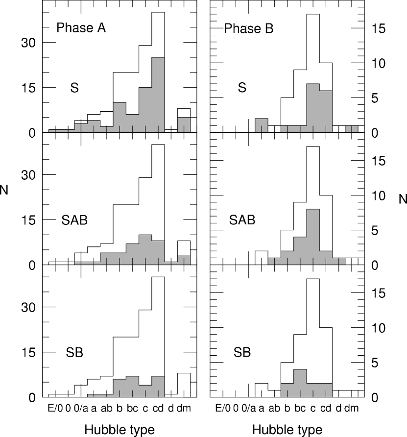
Figure 8: Distribution of Hubble types in Phase-A (left) and Phase-B (right) samples, broken down by un-barred (S), weakly-barred (SAB), and barred (SB) systems (grey histograms). Open histograms represent the total sample for all families; these are identical for the three panels in each column.

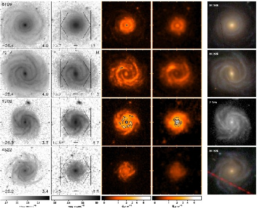
Figure 9: Montage of Phase-B Spitzer sub-sample, sorted by $K$-band absolute magnitude, one line per galaxy. Images from left to right: KPNO 2.1m $B$-band, POSS-II red band used for sample selection, Spitzer/IRAC 8 $\mu$m, Spitzer/MIPS 24 $\mu$m, SDSS false-color (when available) or KPNO 2.1m $B$-band, as indicated by label. (For UGC 72 neither 2.1m nor SDSS images were available; here a POSS-II blue image was used.) SDSS images are SkyServer g’r’i’ (3-band) composites. Right-most images are scaled to 50$\times$50 kpc rasters; all other images are 2$\times$2 arcmin rasters. Gray- and color-scale calibration in mag arcsec^-2 or MJy sr^-1 are given at the bottom. Contours in 8 and 24 $\mu$m images are at 4, 8, 16, 32, 64, and 128 MJy sr^-1. In the first column is given the UGC # (upper-left), $K$-band absolute magnitude (lower-left), and $B-K$ color (lower-right). In the second column is given the $R$-band disk central surface-brightness in mag arcsec^-2 (lower-left) and scale length in arcsec (lower-right). SparsePak square footprint (all H$\alpha$ observations; MgI and CaII observations are indicated by “M” and “C” above the upper-right corner of the footprint) and PPak hexagonal footprint (MgI observations) as well as a 5 kpc bar are drawn in the second column [COLOR]

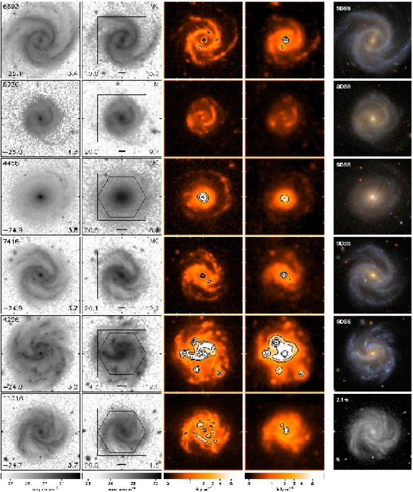
Figure 9: continued [COLOR]

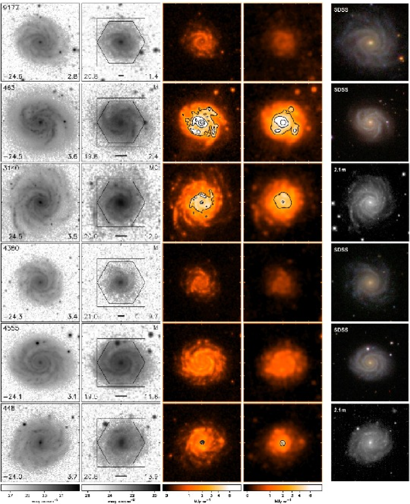
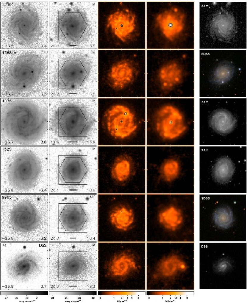
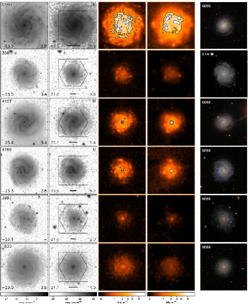
Figure 9: continued [COLOR]

Figure 9: continued [COLOR]

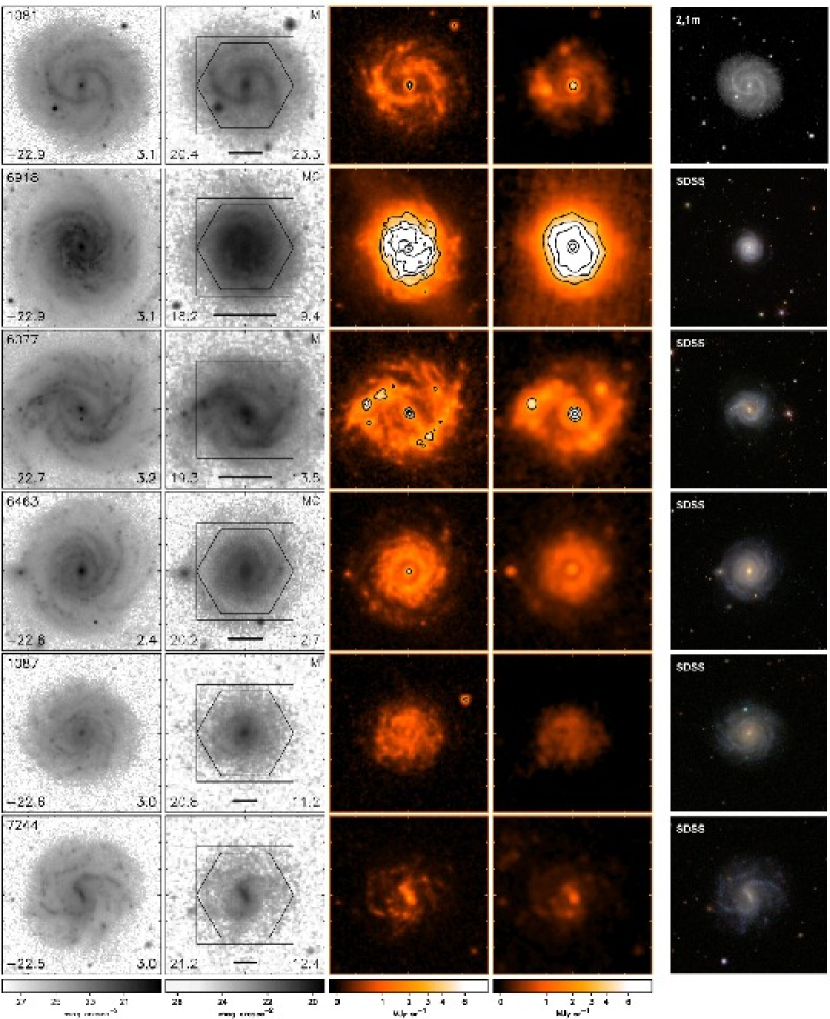
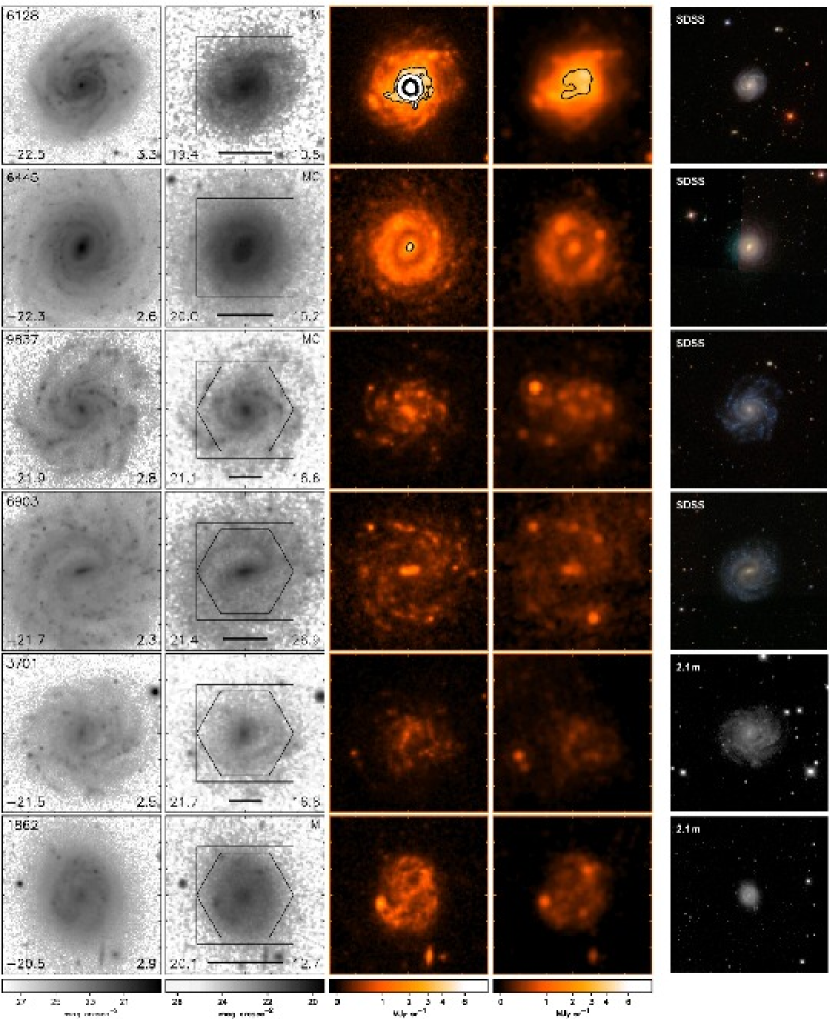
Figure 9: continued [COLOR]

A summary definition of the survey sample, inclusive of our full Phase-A source list, is in Table 2. Coordinates (col. 2 and 3) specify the nominal centers of our IFS observations and Spitzer pointings, where relevant. Morphological types (col. 4) rationalize the independent UGC and RC3 designations. Heliocentric velocities ($V_{\rm hel}$) and distances (D) are adopted from NED (col. 5 and 6); distances use flow-corrections for Virgo, the Great Attractor, and Shapley Supercluster infall. The $B$-band Galactic extinction (col. 7) is based on IRAS measurements (Schlegel et al. 1998), as listed by NED. Apparent $B$-band photometry from RC3 and $K$-band photometry from 2MASS are listed in cols. 8 and 9. These are total magnitudes corrected for systematics which become appreciable beyond $B=13$ and $K=10$ mag (see Appendix A). Absolute $K$-band magnitudes and rest-frame $B-K$ colors (cols. 10 and 11) are corrected for Galactic extinction and distance-modulus only. Our measurements from red DSS images of disk central surface-brightness ($\mu_{0}$) calibrated to the $R$ band, isophotal radius ($r_{23.5}$), disk scale-length ($h_{R}$), and apparent ellipticity are in cols. 12-14. Column 15 indicates how a source was selected to be in the Phase-A sample. The criteria most important for selection in the Phase-A sample are A${}_{B}^{\rm g}$, $h_{R}$ and $r_{23.5}$, in columns 7, 13, 14, respectively. Columns 16-19 report relevant observations for Phase-A and Phase-B portions of the survey, including H$\alpha$, Mg IB-region or Ca II-region spectroscopy, Spitzer imaging, and H I imaging. Sources with stellar spectroscopy, H I, or Spitzer imaging are part of the Phase-B sample. The distribution of Hubble types, barred, weakly-barred, and un-barred for both Phase-A and Phase-B samples is shown in Figure 8. The Phase-B sample observed with Spitzer, representative of our full sample, is shown in Figure 9.

5.2 Sample Characterization

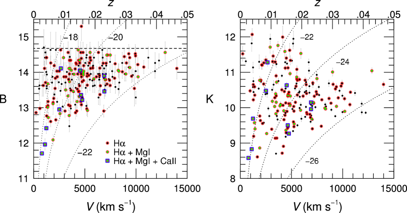
Figure 10: Hubble diagrams for the DMS in the $B$-band (left) and $K$-band (right). Sub-samples are marked according to the key: black points (Phase-A sample); red-encircled points (H$\alpha$ sample); green-cored points (Phase-B Mg IB sample); blue-ensquared points (Phase-B Ca II sample). Objects in the Mg IB sub-sample are also in the H$\alpha$ sub-sample; objects in the Ca II sub-sample are also in Mg IB and H$\alpha$ sub-samples. Dotted lines of constant luminosity are marked. The $B$-band completeness limit of the UGC is delineated with a horizontal dashed line in the left panel. [COLOR]

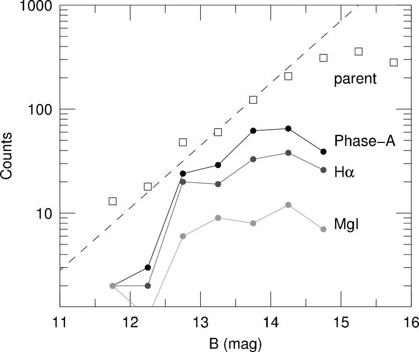
Figure 11: $B$-band galaxy counts (per 0.5 mag) for sub-samples in our survey selected from the UGC. The dashed line has a Euclidean slope of 0.6 dex, with an arbitrary normalization. The curved marked “H$\alpha$” represents the Phase-A sample with H$\alpha$ IFS. The curve marked “MgI” is the subset of the Phase-B sample with Mg I IFS.

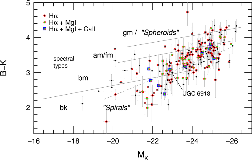
Figure 12: Optical–near-infrared color–absolute-magnitude diagram for the DMS, with sources marked as in Figure 10. Trends for spirals, spheroidals, and galaxies classified by spectral type from Bershady (1995) are marked with lines over the observed luminosity range in that survey, and labeled for reference (see text). The location of UGC 6918 is marked. [COLOR]

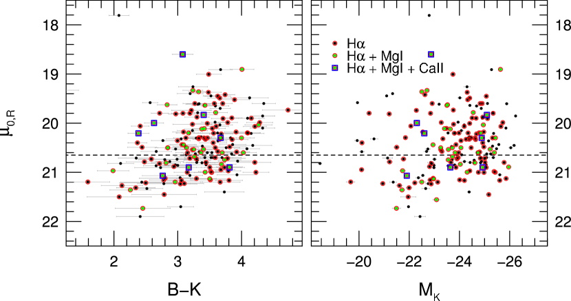
Figure 13: Distributions in $B-K$ color, $K$-band absolute magnitude, $M_{K}$, and red disk central surface-brightness, $\mu_{0,R}$ for the DMS, with sources marked as in Figure 10. The approximate Freeman surface-brightness is indicated by the horizontal dashed line. [COLOR]

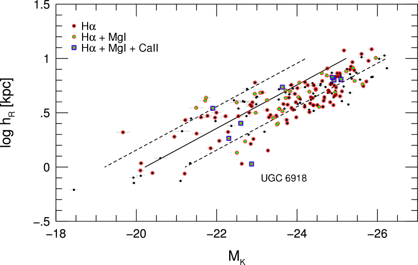
Figure 14: Size versus luminosity for the DMS, with sources marked as in Figure 10. Size corresponds to the disk scale-length, $h_{R}$, measured on red POSS images. Luminosity is measured in the $K$-band. Diagonal lines correspond to constant mean surface-brightness assuming disks dominate the integrated luminosity for Freeman surface-brightness disks of color $B-K=2.3$, 3.3, and 4.3 (left to right, respectively). [COLOR]

We make a provisional photometric characterization of our Phase-A and Phase-B samples in Figures 10-14 based on the tabulated redshifts, $B$ and $K$-band photometry corrected from the literature, and our central disk surface-brightness measurements. A numerical summary of properties is given in Table 3. Figure 10 shows the Phase-A and Phase-B samples have recession velocities of 200-14,000 km/s and $B<14.7$ (the UGC completeness limit). This corresponds roughly to $K<12$. The one source (UGC 3965) fainter than the UGC $B$-band limit is a broad-lined AGN, and presumably faint in the RC3 photometry due to variability. Distances range from 1.3 to 200 Mpc for the Phase-A sample and 18 to 178 Mpc for the Phase-B sample, although 90% of all these samples are contained between 19 and 135 Mpc, with median distances of 62 and 65 Mpc for the Phase-A and Phase-B samples, respectively.

While our Phase-A and Phase-B samples all lie within the nominal completeness limit of the UGC, the samples are not strictly magnitude-limited. This is illustrated in Figure 11, which shows the $B$-band counts for the parent, Phase-A, and Phase-B samples. While the parent sample shows a close-to-Euclidean slope of 0.6 dex for $B<14$, the other samples are substantially sub-Euclidean. In otherwords, our selection of Phase-A and Phase-B samples has preferentially excluded the fainter sources from the parent sample. Nonetheless, like magnitude-limited samples, both the Phase-A and Phase-B luminosity distributions both peak in $B$ and $K$ bands near $M^{*}$, truncating quickly $\sim 2$ magnitudes brighter than this peak, but with extended tails to lower luminosities. The median luminosity values also vary little between sub-samples, in the range of -20.5$\pm 0.1$ and -23.8$\pm 0.2$ for$M_{B}$ and $M_{K}$ respectively. The full luminosity range of the Phase-A sample spans a factors of $10^{4}$ in $L_{B}$ and $L_{K}$, a large fraction of which is due to one extreme low-luminosity source (UGC 7414) at low heliocenteric velocity. This source has relatively large flow-corrections, and hence its distance and luminosities are uncertain. A more robust characterization is based on the luminosity range enclosing 90% of the Phase-A sample; this spans factors of $>$40 in $L_{B}$ and $>$150 in $L_{K}$. The full range of luminosties for the Phase-B sample, which does not include UGC 7414, span factors of $\sim$55 in both $L_{B}$ and $L_{K}$. In short, the sample spans about a factor of 100 in $L_{K}$, which should correspond to a comparable range in stellar mass.

The optical–near-infrared color-luminosity distribution in Figure 12 shows the DMS spans a wide range of disk types. Both the Phase-A and Phase-B samples’ colors range from $2.0<B-K<4.25$, or about a factor of 8 in $L_{B}/L_{K}$. The subset with Ca II-region IFS spans only a factor of 4 in $L_{B}/L_{K}$, but is well dispersed within the color-luminosity distribution. The range of rest-frame colors spans galaxy spectral types (Bershady 1995) from bk through gm, i.e., galaxies dominated by the light of B+K stars through G+M stars. The regressions shown in Figure 12 have been converted to our adopted cosmology and photometric band-passes. For example, consistent with the analysis presented in §4.3.2 (Figure 7), UGC 6918 is a bm-type galaxy, close to the boundary for bk-type galaxies, i.e., well-represented by a 3-star admixture of B+K+M stars. The wide range of spectral types indicates a wide range of stellar populations are present in the sample, well-suited for probing variations in $\Upsilon_{\ast}$ and their putative correlations with color.

While the DMS sample is not complete in any quantitative sense, it samples well the population of luminous spiral galaxies in the nearby field. The sample color-luminosity distribution matches the trends seen in deeper fields samples, e.g., the $B<20.5$ sample from Bershady et al. (1994), but is absent the low-luminosity (dwarf) systems ($M_{K}>-20.5$) at blue color ($B-K<3$). Consequently, the distribution follows the ridge-line for spirals seen in brighter surveys (labeled “Spirals” in Figure 12) corresponding to $M^{*}$ that decreases with later galaxy types.

There are the 17 galaxies within 0.2 mag (or redder) of the red-sequence (labeled here gm or “Spheroids”). By definition of the sample, this is not due to inclination-effects. Of these, 12 galaxies are morphologically classified as Sab or earlier, i.e., bulge, or spheroid-dominated systems. One lying well above the red-sequence is the broad-lined AGN noted above. Of the remaining 5 galaxies, 3 are classified only as “S”, but visual inspection reveals systems with either a large bulge (UGC 7205), of very early type (UGC 9610; a barred S0), and possibly a dusty star-burst (UGC 12418). The other two galaxies are classified as Sb or Sbc systems, lie slightly below the red sequence, and hence are consistent with the tail of the intermediate-spiral distribution.

Finally, the disk central surface-brightness distribution is shown in Figure 13 versus $B-K$ color and $M_{K}$. The well-known but weak trends to lower surface-brightness at bluer color and lower luminosity are seen. Size and luminosity are tightly correlated in the sample (about a factor of 3 range in size at given luminosity; Figure 14), while size and surface-brightness are not. The full Phase-A and Phase-B samples span a factor of 35 in surface-brightnesses about the Freeman value. The surface-brightness range enclosing 90% of these samples span 3.5 times higher and two times lower than the Freeman value. In general, the subset of Phase-B galaxies well-samples the full Phase-A distribution, except at luminosities $M_{K}>-21.5$. The survey as a whole selects against low surface-brightness disks. This is a result of our size limit coupled with the depth limitations of the UGC. The resulting samples are well matched to the observational capabilities of current instrumentation, and still probe a wide range in disk surface-brightness. In comparison (cf. Table 3), Bottema’s (1997) sample spans a similar range in surface-brightess ($\mu_{0}=20.25^{+1.2}_{-0.8}$ in the $R$ band), color ($B-K=3.5^{+0.8}_{-0.5}$), and luminisity ($M_{K}=-23.6^{+1.9}_{-1.5}$).

Given the complex structure and large dynamic range of spiral-galaxy light-profiles, there were significant instances where the automated surface-photometry fitting described in §5.1 failed to provide an adequate description of the disk radial and luminosity scales. Typically this was because a light profile showed evidence for inner breaks (type I and II luminosity profiles; Freeman 1970) and/or outer breaks (Pohlen & Trujillo 2006). In these cases we redid the fitting after identifying the radial region outside of an inner break corresponding to the extent of the SparsePak footprint. The disk central surface-brightness and scale-length values in the figures and Table 2 reflect values from the updated fits. Even these updated fits are only an exponential characterization of the light profile within the region where we have measured gas and stellar kinematics. In the table we flag the three cases where the updated values place the source outside of the DSS-sample selection definition.

6 OBSERVATIONS

6.1 Total and Gas Masses

The kinematic data used to dynamically determine the total mass distribution come from two-dimensional velocity-fields measured in H$\alpha$ and H I. We summarize the basic observations, and indicate how the data are used.

6.1.1 H$\alpha$ Integral-Field Spectroscopy

H$\alpha$ kinematic data were taken with the SparsePak IFU in the echelle configuration specified in Table 1. We observed 137 galaxies over 13 runs from January 2002 to April 2005 totaling 41.5 nights, plus portions of two additional runs totaling 8 nights during SparsePak commissioning in May-June 2001. As noted above, 14 galaxies in the survey had prior observations using DensePak, a similar IFU, and essentially the identical spectrograph configuration. Eight of these were not re-observed with SparsePak.

Relevant science data include a 3-position dither-pattern for H$\alpha$ to create a filled-in map, although in some cases this was not achieved. With a completed, 3-position pointing, the fill-factor is $\sim$65%. Galaxies without 3 pointings or observed in poor conditions are flagged as “low quality” in Table 2, regardless of the detected signal level. Of the 20 galaxies (13%) with low-quality H$\alpha$ data, only four are in the Phase-B sample, and only three are in the Spitzer sub-set. Regardless, the H$\alpha$ data available are sufficient for velocity-field modeling of all Phase-B sources. The typical extent of the velocity field reaches to between 2 and 4 disk scale-lengths.

The basic analysis of the H$\alpha$ spectra consists of preliminary processing, characterization of all the nebular lines in the echelle order (H$\alpha$, [N II]$\lambda\lambda$6548,6583, and often the sulfur doublet [SII]$\lambda\lambda$6717,6730), and estimating the spectral continuum. Preliminary processing (extraction, rectification, and calibration) was carried out with standard routines found in IRAF. Minor parameter modifications particular to the SparsePak data format, as well as alternative sky-subtraction methods are detailed elsewhere. Line-fitting is done with a custom-built code which fits single and double Gaussians to each profile, deriving line strengths, centroids, and widths, as well as accurate errors (Andersen et al. 2006, Andersen et al. 2008). Lines with strong skew, bimodality, or unusually large widths are identified.

These basic data products allow us to measure inclination, rotation speed, and kinematic regularity using velocity fields generated from line centroid maps; to spatially register the bi-dimensional spectroscopic data both in a relative and absolute sense (Paper II) using continuum and velocity maps; to estimate star-formation rates from H$\alpha$ equivalent widths calibrated with broad-band photometry; and to crudely estimate metallicity using [N II]/H$\alpha$ line ratios. These results will be part of the DMS paper series. A full description of the observations, reduction and basic analysis of the emission-line profiles are presented in Swaters et al. (2010, in preparation) and Andersen et al. (2010, in preparation).

6.1.2 H I Aperture Synthesis Interferometry

Aperture-synthesis radio observations at 21 cm have been obtained to determine H I velocity fields, from which extended rotation curves can be derived to supplement the H$\alpha$ kinematic data, and to map the surface density of the cold neutral gas. In total, 43 galaxies have been imaged in H I with either the VLA in its C-short configuration (7 galaxies in 2005), the WSRT (20 galaxies in 2007-2009, 3 overlapping with VLA), or the GMRT (19 galaxies in 2008-2009, 1 overlapping with VLA and WSRT, 2 others overlapping with WSRT). Integration times were typically 5 to 12 hours per source, with minimum synthesized beams between 5 arcsec for the GMRT and 15$\times$30 arcsec for lower-declination sources observed with the WSRT. After Hanning smoothing, the FWHM velocity resolutions are 10.3, 4.1 and 13.2 km s^-1 for the VLA, WSRT and GMRT respectively. The column-density sensitivities of the data, smoothed to $\sim$15 arcsec angular resolution and $\sim$12 km s^-1 velocity resolution, is 2 to 5$\times 10^{20}$ atoms cm^-2 at the 5$\sigma$ level. The observed galaxies are indicated in Table 3 with V, W, or G, respectively, according to the facility used. All 43 galaxies with high-quality H$\alpha$ and stellar kinematic IFU data, and all 41 galaxies with Spitzer imaging data thus have 21-cm aperture-synthesis observations available (Martinsson et al. 2010, in preparation).

6.2 Disk Mass Surface-Density

The kinematic data critical to dynamical estimation of the disk mass surface-density ($\sigma_{z}$) comes from the two-dimensional velocity- and velocity-dispersion fields measured in the Mg IB and Ca II regions. Below, we summarize the primary galaxy and stellar template observations.

6.2.1 Mg IB and Ca II integral-field spectroscopy

Stellar kinematic data were collected with both the SparsePak and PPak IFUs. SparsePak stellar line-of-sight velocity dispersion ($\sigma_{\rm LOS}$) observations were taken over 17 runs totaling 58 nights, plus portions of 4 other runs totaling 11.5 nights. Six of these runs were used to gather Ca II data, mostly during the pilot program from May 2001 through May 2002. SparsePak Mg IB data were gathered from April 2005 to April 2007. PPak stellar $\sigma_{\rm LOS}$ observations were taken in Mg IB only, over 12 runs totaling 48 nights from March 2003 to January 2007. Combined with the Phase-A H$\alpha$ observations, the spectroscopic campaign used $\sim$160 nights of 4m-class telescope time over 6 years.

Of the 46 galaxies observed with stellar IFS, 19 were observed in the Mg IB-region with both SparsPak and PPak (10 of which have high-quality data from both instruments). This overlap serves to cross-check $\sigma_{\rm LOS}$ derived from different instruments, and enables us to assess the impact of instrumental artifacts. In these cases, the data can also be combined to increase the depth. Of the 9 galaxies with Ca II-region IFS, 5 are of high-quality, and the additional 4 galaxies have high-quality Mg IB-region IFS.

Relevant science data include deep, multi-exposure, single-position galaxy pointings for Mg IB and Ca II-triplet spectral regions and short template-star observations (below). In contrast to the H$\alpha$ observations, we did not attempt to create a filled-in map for the galaxy observations since wherever possible we hoped to be able to combine the multiple exposures and maximize S/N in individual fibers at a single position. Spatial registration of these data use the same methods employed with the H$\alpha$ data (see Paper II). Given the limited spectral range wavelength of our configurations, quartz-lamp dome-flats served to provide a relative flux calibration to the spectra (to within a few percent), as verified by observations of spectrophotometric standards. This is adequate for preserving the shape of the spectral continuum in both template and galaxy data, useful for template fitting in direct-wavelength or cross-correlation approaches.

Basic spectroscopic data processing was similar to that used for the H$\alpha$ IFS observations. Modifications were made to implement flexure-corrections in the PPak data (Martinsson et al., in perparation; PMAS is a Cassegrain-mounted spectrograph), and to improve sky-subtraction (see Bershady et al. 2005, Paper II, and future papers in this series). Considerable attention was paid to estimating errors in the extracted spectra by carefully accounting for the spectral trace and the known detector properties of read-noise and gain. Corrections for scattered-light in the spectrograph optics have not been made to the data, although they are appreciable in the Ca II data (see Bershady et al. 2005). The two-dimensional nature of the scattering effect in SparsePak data is to add a small, featureless continuum to the observed spectra, which should have no impact on the derived velocity information.

6.2.2 Stellar templates

Roughly 150 template stars were observed in the same instrumental configurations as the source observations for Mg IB and Ca II regions, except stars were intentionally drifted across roughly a dozen fibers in the course of an exposure. This procedure allows us to sample a range of fibers to test for effects of varying instrumental resolution (see Paper II), and also to illuminate the fibers in a fashion more similar to the near uniform illumination during target exposures of galaxies (see Bershady et al. 2005).

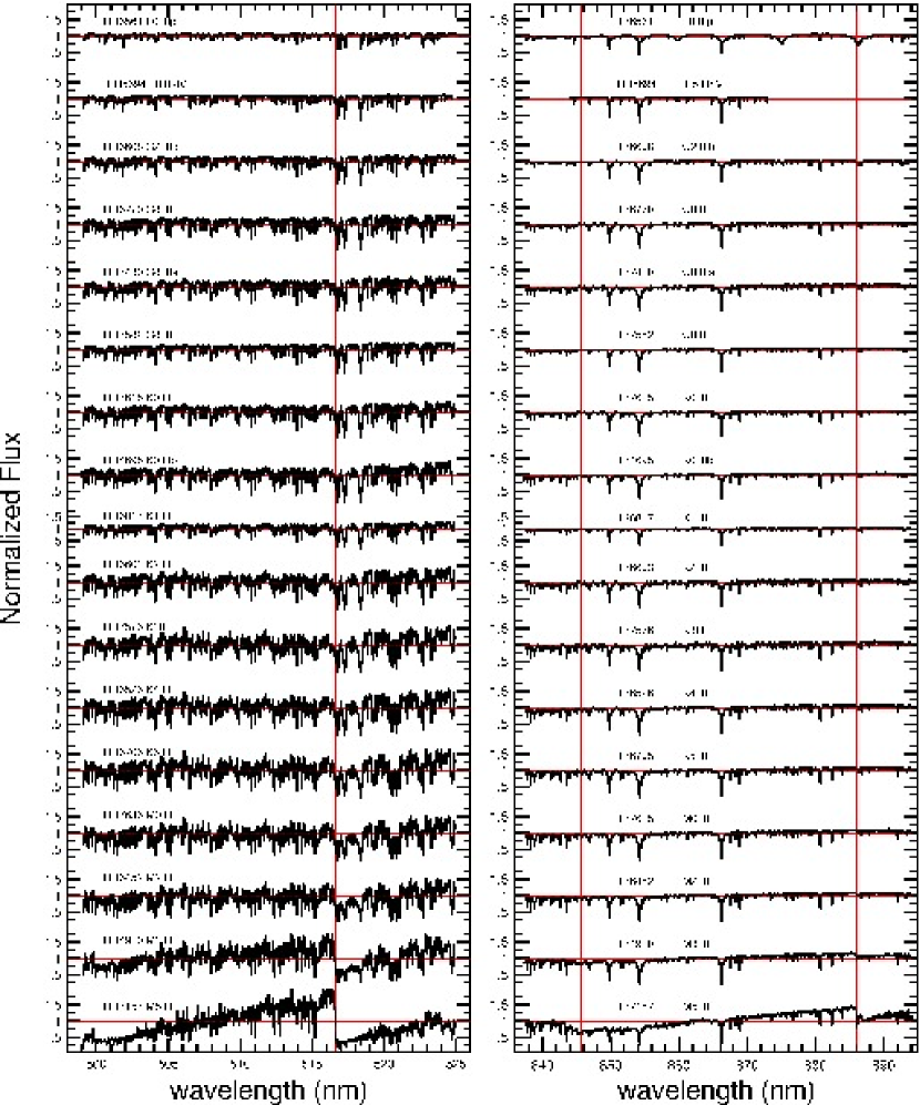
Figure 15: SparsePak template subset for luminosity-class II-III and spectral types F0 to M5. Spectra are normalized to unity mean. Vertical lines mark molecular band-heads. [COLOR IN ELECTRONIC EDITION ONLY.]

The template library began with roughly 3-dozen stars with a wide range of T (3000-20,000 K) and surface-gravity (luminosity classes I-V), with some emphasis on giants (class III) in the late-F through late-K spectral range, taken during SparsePak commissioning in May and June 2001. Subsequent observations of 47 stars with SparsePak have extended our template library to include more metal-poor stars, particularly giants, expanding the dynamic range in metallicity from -2.1$<$[Fe/H]$<$0.3. With PPak, 72 stars were also observed, 13 hot stars (B-F, luminosity class I-V) with -0.75$<$[Fe/H]$<$+0.15, and 59 cool stars (G-M, luminosity class III or IV) with -1$<$[Fe/H]$<$+0.35. These include repeat observations to established estimates of systematic errors due to subtle changes in instrumental configuration (e.g., focus). A subsample of giant stars in our library most relevant for our cross-correlation analysis in Paper II are shown in Figure 15 for both Mg IB and Ca II regions. Note that by mid-F and hotter the line-strengths become appreciably weaker, while in the Ca II region the Paschen-series begins to dominate. At cooler temperatures both the Mg IB and Ca II regions display strong TiO band-heads, appearing prominently in the Mg IB region starting at K5, and in the Ca II region at M3.

6.3 Star-formation, Stellar Populations, and the Interstellar Medium

We summarize the optical–NIR imaging and Spitzer observations taken to characterize stellar emission and the dusty interstellar medium. Combined with our IFS and H I observations, these provide estimates of the bolometric star-formation rate, the energetics of the ISM, and a stellar populations inventory – all a framework for interpretation of our dynamical $\Upsilon_{\ast}$ estimates.

6.3.1 Optical and NIR Imaging

Deep $UBI$ and shallow $VR$-band imaging data were obtained using the KPNO 2.1m telescope for nearly all galaxies with H$\alpha$ IFS data, and for the entire Phase-B sample. Typical exposure times were 600 sec in $U$, 300 sec in $B$, 60 sec in $V$ and $R$, and 1200 sec in $I$. Seeing ranged from 0.9 to 1.8 arcsec FWHM, with 1.4 arcsec a typical value. The optical data were acquired using the T2KA CCD detector (2048², $10.2\times 10.2$ arcmin field, 0.305 arcsec pixel^-1) over 4 runs totaling 26 nights. $B$-band images are illustrated in Figure 9.

Deep $JHK$-band images were obtained for two thirds of the galaxies with H$\alpha$ IFS data, again including all of the Phase-B sample. These data were acquired with the same telescope and the SQIID quad-channel imager (four 1024² InSb arrays, each with $440\times 460$ pixels active, $5.07\times 5.28$ arcmin field, 0.69 arcsec pixel^-1) over 6 runs totaling 35 nights. Observations were taken by dithering the telecsope in a 3 by 3 grid so that the galaxy image would fall at different locations within the unvignetted field of view. This dither sequence was repeated three times for each galaxy, slightly offsetting between cycles. Typical exposure times were 2160 sec, but the effective exposure time in the combinned dithered data decrease towards the edges. Seeing ranged from 0.8 to 1.5 arcsec FWHM, with 1.2 arcsec a typical value.

6.3.2 Spitzer Space Telescope Imaging

Measurements were designed to be efficient, complementing and utilizing the more detailed Spitzer measurements of, e.g., the SINGS Legacy program. We restricted observations to 4.5, 8, 24, and 70 $\mu$m imaging with IRAC and MIPS. Spitzer is a 0.85m telescope, diffraction limited at wavelengths longward of 5.5 $\mu$m. Detector pixels critically sample the diffraction core, except at 4.5 $\mu$m, where the data is undersampled. The 4.5 and 8 $\mu$m IRAC flux maps, sampled at $\sim$1.2 arcsec pixel^-1, combined with $JHK$ ground-based surface-photometry are intended to allow us to disentangle stellar photospheric emission from PAH contributions. The 8, 24, and 70 $\mu$m fluxes, sampled respectively at $\sim$1.2, 2.5, and 10 arcsec pixel^-1, aim to allow us to characterize the amplitude and temperature of the warm dust. The correlation of 24 $\mu$m fluxes to star-formation rates can be compared directly with our H$\alpha$ and H I measurements in matched apertures.

Our depth was targeted to give reliable surface-photometry out to three optical disk scale-lengths, matching the extent of the kinematic measurements constraining total disk mass-densities. Exposures aimed to reach S/N of 3 per spatial resolution element at 3 $h_{R}$, a depth comparable to SINGS. Based on Dale et al. (2005), we estimate average flux levels to be $0.025\pm 0.005$ MJy sr^-1, $0.14\pm 0.04$ MJy sr^-1, $0.15\pm 0.03$ MJy sr^-1 and $1.4\pm 0.4$ MJy sr^-1 at 4.5, 8, 24. and 70 $\mu$m, respectively. Exposures were 360 sec for IRAC 4.5 and 8 $\mu$m, 333 sec for MIPS 24 and 75 sec for MIPS 70 $\mu$m measurements, totaling 26.3 hours of telescope time for 41 galaxies. Images at 8 and 24 $\mu$m are illustrated in Figure 9.

Of the galaxies in our DMS Spitzer sample – a subset of the Phase-B sample described in §5.1 – all of them have high-quality H$\alpha$ spectroscopic and H I imaging observations, all but one have high-quality Mg IB-region stellar absorption-line spectroscopy.

7 METHODS OF ANALYSIS

The many components of the DMS analysis are described in future papers in this series, but two methods stand out: kinematic inclinations for nearly face-on galaxies, and stellar velocity dispersions at low surface-brightness for composite stellar populations. Because of their central importance, these are outlined here.

7.1 Inclinations

7.1.1 Kinematic Inclinations and Position Angles

Our technique for determining kinematic inclination and position angle (PA) employs fitting a single, tilted disk to all the H$\alpha$ velocities across the face of each galaxy, i.e., one zone, and a functional form for the trend of rotation speed versus radius. In some cases, where there is clearly a strong bar or oval distortion in the inner region, a two-zone model is used. The detailed functional form of the rotation curve is unimportant to the derivation of PA and kinematic inclination so long as it is sufficiently flexible to account for the observed range of radial shapes. The technique, developed by Andersen (2001), and used with similar data in Andersen et al. (2001, 2003), is similar to tilted-ring fitting. The advantage of limiting the number of radial zones is to provide enough data points to precisely constrain a model parameterization of the rotation curve.

To apply these values to the stellar data we make the reasonable assumptions that the gas and stars are co-planar and share the same barycenter. A detailed description of the method as applied to the DMS will be presented in Andersen et al. (2010, in preparation). Preliminary estimates of the performance in terms of inclination random error are given in Paper II. The zero-point and slope of the nearly face-on TF relation based on kinematic inclinations using this method (Andersen & Bershady 2003) is consistent within the uncertainties for the same quantities for more inclined samples, demonstrating there are no significant systematic errors.

7.1.2 Inclinations from Scaling-Relation Inversion

Disk inclination can also be estimated by inverting the TF relation (Rix & Zaritsky 1995), assuming survey galaxies lie along a fiducial relation established with galaxies of similar type that have reliable kinematic or photometric inclinations. So-called inverse Tully-Fisher (iTF) inclinations have the advantage that their errors decrease with inclination. Inclination from iTF are only effective if a precise measure of the projected rotation velocity can be obtained. This requires measuring a rotation curve rather than an integrated line-width in order to (a) avoid confusion between rotation and turbulent motion, and (b) verify the regularity of the velocity field and its asymptotic flatness at larger radii (see discussion in Verheijen 2001). The smaller the scatter in the TF relation, the more precise the iTF-based inclination estimates.

The combination of high spectral-resolution IFS and near-infrared photometry allows us to make the best possible inclinations estimates from iTF. As Figure 16 illustrates for a very-nearly face-on galaxy in our survey, whatever the true inclination and circular speed, our spectroscopy has the resolution and spatial coverage to determine that this galaxy has a very regular velocity field and flat asymptotic rotation curve. The smallest observed scatter in the TF relation requires near-infrared luminosities and verification of asymptotically-flat, regular velocity fields (Verheijen 2001).

Despite this promise of high precision, using iTF remains a potentially fatal path if used in isolation because its accuracy is not verifiable a priori. Our preference is to work in a regime where kinematic inclination errors are small enough to verify a galaxy’s location on the Tully-Fisher relation. We will, however, take advantage of the iTF method to reduce errors in some situations, depending on the observed regularity of the ionized-gas velocity fields.

7.2 Stellar Velocity Dispersions

To arrive at the kinematic line-width required to estimate the disk mass surface-density, two steps are needed. First $\sigma_{\rm LOS}$ must be derived from the spectroscopic data, and second $\sigma_{z}$ must be deprojected from the former line-of-sight quantity.

There is a considerable variety of methods for determining $\sigma_{\rm LOS}$ from the integrated star-light of galaxies, but the methods basically fall into the two categories of direct-fitting and cross-correlation. In the former, galaxy spectra are fit directly in wavelength space, with a template that is optimized for suitability both in terms of velocity broadening and spectral match. We adopt, instead, a new application of the cross-correlation approach (Paper III; Westfall 2009). As we demonstrate in Papers II and III, our method not only optimizes the determination of the primary measure of interest (broadening), but allows us to minimize template mismatch as well as, if not better than, direct-fitting methods.

Within this cross-correlation context, we have considered two complementary approaches to deriving $\sigma_{z}$ from our line-of-sight measurements, each taking different advantages of the bi-dimensional nature of our spectral coverage. Specifically, these approaches either minimize systematics due to S/N and template-mismatch associated with determining $\sigma_{\rm LOS}$, or mimize systematics associated with deprojecting the SVE to find $\sigma_{z}$.

The first approach is to average fibers at a given radius over azimuth (i.e., in a ring), correcting for their velocity offsets due to projection of the internal velocity field, derive the broadening function $\sigma_{\rm LOS}$ for the registered and combined spectrum at each radius, and correct for line-of-sight projection of $\sigma_{R}$, $\sigma_{\theta}$, beam-smearing, and instrumental resolution.

The number of fibers in an annulus range from 6-30 for SparsePak when the radial width of the fiber-centers is constrained to be of order the fiber diameter (Figure 4). Comparable-width annuli for PPak include up to 120 fibers, but thinner annuli can be defined when the S/N is high enough. The advantage of fiber-averaging is that higher S/N is achieved before the cross-correlation (or direct fitting) process to derive $\sigma_{\rm LOS}$. The benefits are severalfold. Higher S/N enables better, direct inspection as well as quantitative assessment of goodness of fit, particularly in terms of template mismatch. In contrast, only velocity information is required from individual fibers in order to velocity-register the spectra, which is much easier to derive at low S/N, and is rather immune to template mismatch. We show in Paper II that this registration is quite robust when assisted with prior empirical knowledge based on, e.g., the gas or stellar rotation curve. Higher S/N also helps ensure that any noise-dependent systematics in estimating $\sigma_{\rm LOS}$ are minimized, although we have not found such systematics to be present at a significant level for S/N$>3$ pix^-1 (see Papers II and III). A further advantage is that the derived $\sigma_{\rm LOS}$ at any one radius relative to another is independent of model assumptions, e.g., on the radial form of $\sigma_{z}$. The only disadvantage is that some prior knowledge of the SVE must be known in order to decompose $\sigma_{\rm LOS}$ to find $\sigma_{z}$.

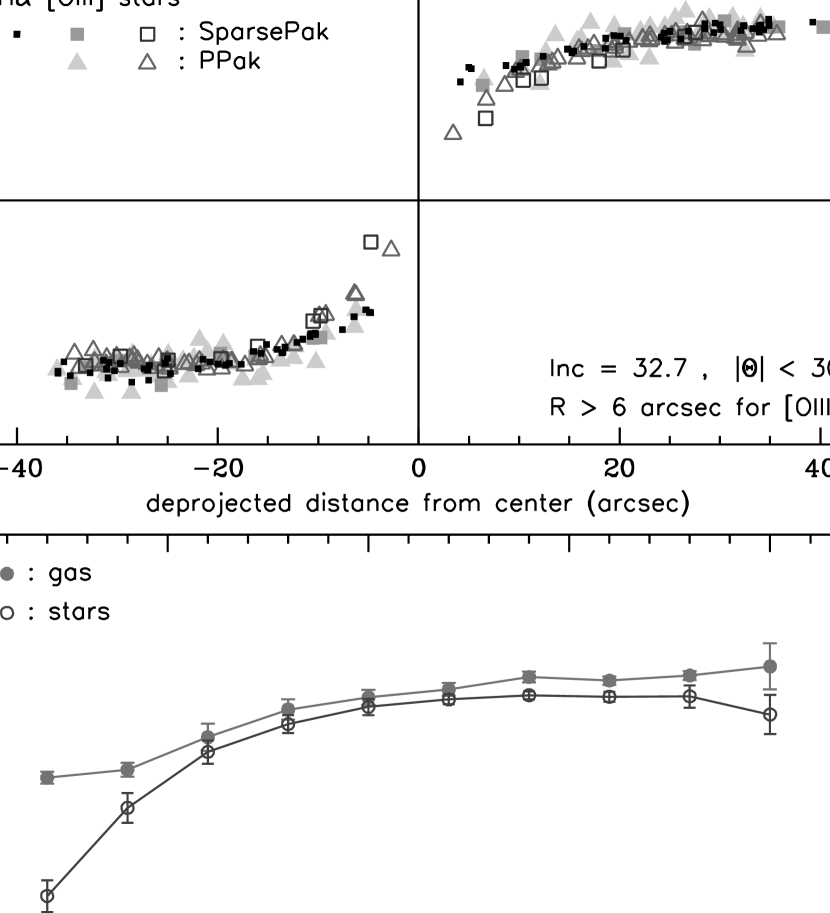
Figure 17: Asymmetric drift between the de-projected tangential velocities of stars (open squares and triangles) and ionized gas (filled grey squares and triangles for [O III]$\lambda$5007; small, filled squares for H$\alpha$) in UGC 6918, as observed with SparsePak and PPak. Gas velocities are based on line centroids, while stellar velocities are from cross-correlation with stellar templates in the same (Mg IB) spectral region. The top panel shows deprojected tangential velocities for individual fibers within 30^∘ of the kinematic major axis, adopting a kinematic inclination of 32.7^∘, and corrected for the systemic recession velocity, $V_{\rm sys}$. The bottom panel gives the amplitude of the deprojected tangential velocity for gas and stars, $V_{\rm rot}$, derived from tilted ring fits to radial bins of fibers, adopting the same inclination for each bin, and combining all SparsePak and PPak data shown in the top panel.

To handle this short-coming, we have devised a second approach, described in Westfall (2009) and Westfall et al. (2010, in preparation), which treats the fibers separately, in that their $\sigma_{\rm LOS}$ is determined individually (e.g., by cross-correlation). There is ample signal in inner regions of most galaxies (typically out to 1 to 2 disk scale-lengths) to examine the velocity broadening in this way. By preserving the two-dimensional information on $\sigma_{\rm LOS}$, we may solve directly for the SVE by imposing at least one other constraint. The most powerful constraint is dynamical, and arises from the asymmetric-drift equation. This takes full advantage of the direct observations of the lag between the projected tangential velocity between gas and stars, as illustrated in Figure 17 for UGC 6918. This lag, akin to the so-called asymmetric-drift observed in the Milky Way, is an interesting and dynamically significant measure in its own right. Figure 17 demonstrates the repeatability of our velocity measurements at different wavelengths (513 and 670 nm), with different instruments (SparsePak and PPak), and different tracers (gas and stars). Moreover, the quality of the velocity-centroid measurements are high enough and the velocity-fields are regular enough to reveal asymmetric-drift at levels of 5 to 10 km s^-1, well below our instrumental resolution.

Further dynamical constraints include the epicycle approximation, and other equations that establish a covariance between any two axes of the SVE, e.g., constant vertical-anisotropy ($\sigma_{z}/\sigma_{R}$ constant), or constant disk stability. Radial parameterizations are also of aid in solving for the trend in the SVE amplitude and shape. Westfall (2009) describes the various possible methods in detail, and demonstrates their application. The key advantage of this approach is the direct measure of the SVE shape, which we find is fairly robust to different dynamical assumptions and parameterizations. Further, individual fiber measurements allow for higher spatial resolution of $\sigma_{\rm LOS}$. In particular, the azimuthal structure can be sensitive not only to the changing SVE projection but spiral structure. However, the impact of template-mismatch is difficult to assess given the limited S/N of individual fiber spectra, the radial range of analysis is similarly limited, and the parameterization of the SVE as well as the use of dynamical assumptions has the potential to introduce systematic errors.

On balance, the two approaches make different trades in terms of systematic and random errors, and therefore are best used together, in an iterative sense, respectively probing template mismatch and the SVE shape. Paper II describes the elements critical to the first (fiber-averaging) approach. This is useful for visualizing the quality of the spectral data, and it is used to estimate the survey error budget.

8 SUMMARY

We have argued that the disk-halo degeneracy, central to obstructing a reliable mass decomposition based on the rotation curves of spiral galaxies, is unbreakable without independent information about either the halo or disk mass, or a combination of the two. Despite the long-known limitations of using rotation curves to place limits on $\Upsilon_{\ast}$ (van Albada et al. 1985), namely that only upper limits may be set (the maximum-disk hypothesis), the literature abounds with efforts to use rotation curves to place stronger constraints on $\Upsilon_{\ast}$, dark-matter halo parameters, or worse – both. The uncertainties do not go away with better data (e.g., de Blok et al. 2008) or with two-dimensional fitting. This is because galaxies are intrinsically non-axisymmetric at a level (5-10 km s^-1 or more; Trachternach 2008) required to discern either significant differences between low and high values of $\Upsilon_{\ast}$, different halo models, or both. Unfortunately, independent contraints from SPS models on $\Upsilon_{\ast}$ are rather poor (uncertainties of factors of 4, and possibly much larger are likely) due to uncertainties in the low-mass end of the IMF, late-phases of stellar evolution (especially the TP-AGB), and a wide range of possible star-formation and chemical-enrichment histories.

We have described one of several methods in the literature that can be used to break the disk-halo degeneracy, and hence challenge the maximum-disk hypothesis. This method uses measurements of the vertical velocity dispersion of disk stars along with an estimate of the vertical scale height to place direct dynamical limits on the mass surface-density of spiral disks. Advantages of the approach are that it is conceptually simple, it uses collisionless tracers, and it provides direct, spatially resolved information about the mass distribution within galaxies. The measurement was suggested and pioneered 25 years ago (Bahcall & Casertano, 1984; van der Kruit & Freeman 1984). One small, early survey (Bottema 1993) yielded the tantalizing result that normal galaxy disks are substantially sub-maximal ($\sim$50% by mass). However, until recently there have been substantial technical limitations in gathering sufficient signal to measure reliably the velocity dispersions of disk stars at the low surface-brightness levels required to probe well into the disks of normal spirals.

In this context we have given an overview of a new study, the DiskMass Survey, of the mass distribution within normal spirals galaxies. Our approach has been to use custom-built IFUs to measure the stellar and gaseous velocities and velocity dispersion fields in nearly-face on systems close to 30 degrees. Inclinations are low enough to favorably project $\sigma_{z}$, but not too low to prevent kinematic inclinations, and hence total mass estimates to be made based on the observed velocity fields. The sample selection and survey protocol, whereby we down-select targets for ever increasing study, has been detailed here. The resulting data set includes H$\alpha$ velocity fields for 146 galaxies; stellar kinematics in at least one of the Mg IB (513 nm) or Ca II (860nm) spectral regions for 46 of these galaxies; and Spitzer Space Telescope IRAC and MIPS (4 through 70 $\mu$m) imaging as well as 21cm aperture-synthesis imaging for 41 of these 46 galaxies. Observations required $\sim$220 nights of 2-4m aperture ground-based telescope time, 400 hours of 21cm radio interferometry, and 26 hours of Spitzer time. The DMS galaxies span close to an order of magnitude in color and size (surface-brightness), and two orders of magnitude in luminosity. The size and scope of the survey is large enough to make reliable statistical statements about disk maximality and calibrate $\Upsilon_{\ast}$ over a wide range of disk properties.

We have briefly summarized the observations and analysis undertaken for the survey to serve as a road-map to later papers in this series. In a companion paper we present a detailed error budget for disk mass surface-density, mass-to-light ratios and disk mass-fraction (Paper II); a following paper establishes our new cross-correlation method (Paper III). Future papers will present results on topics including, but not limited to, the measurement of total galaxy mass; the Tully-Fisher relation for nearly face-on galaxies; disk kinematic asymmetries, star-formation rates, gas content, mass surface-density, the SVE, and $\Upsilon$; as well as halo density profiles. While a few of these topics will have been explored in greater depth by other surveys (e.g., star-formation; SINGS, Kennicutt et al. 2006), our aim is to complement and extend our knowledge of nearby galaxies by providing an absolute calibration of stellar mass, and a direct inference of the shape of dark-matter halos. This advance, in turn, should extend the bounds of our understsanding of how galaxies have formed and evolved.

Appendix A Corrections for RC3 and 2MASS $B$ and $K$ Total Magnitudes

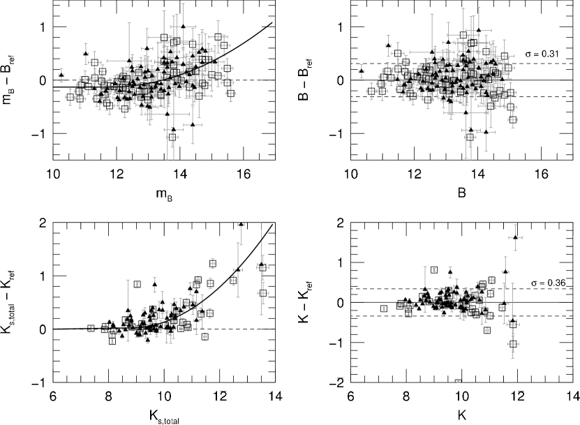
Figure 18: Calibration data for RC3 $B$ and 2MASS $K$ total galaxy magnitudes. Left-hand panels show RC3 $m_{B}$ vs. reference $B$-band photometry (top) and 2MASS $K_{\rm s,total}$ vs. reference $K$-band photometry (bottom). Reference data are from deep surface-photometry of Verheijen & Sancisi (2001; open squares) and de Jong (1994; filled circles). Quadratic fits to deviations are shown as solid lines. Right-hand panels show corrected $B-$ and $K$-band photometry vs. the reference photometry, with dashed lines giving the rms scatter.

The total magnitudes from RC3 and 2MASS, listed in NED as “B (m_B)” (here $m_{B}$) and “K_s_total (2MASS)” (here $K_{\rm s,total}$) have been corrected for systematic effects with apparent magnitude based on comparison to total magnitudes measured for the samples of Verheijen & Sancisi (2001) and de Jong (1994). The latter are based on deep surface-photometry. These corrections, illustrated in Figure 18, are:

$$B\ =\ m_{B}\ -\ 6.18\ +\ 1.08\ m_{B}\ -\ 0.046\ m_{B}^{2}$$ (A1)

$$K\ =\ K_{\rm s,total}\ -\ 5.73\ +\ 1.30\ K_{\rm s,total}-0.074\ K_{\rm s,total}^{2}$$ (A2)

and are applied to the photometry listed in Table 2. We emphasize that these corrections, along with the magnitudes in Table 2 are corrected neither for internal or foreground extinction, or $k$-corrections, and are applicable to extended sources.

Noordermeer & Verheijen 2007 find a surface-brightness dependence to their comparison of the Verheijen & Sancisi (2001) data, but we see no such additional dependence after applying the above corrections. We note that in the Verheijen & Sancisi (2001) sample, which is volume limited, apparent magnitude and surface-brightness are highly correlated.

The dispersions in the corrected values are 0.31 mag for $B$, compared to the mean expected random error of 0.25 mag (0.22 mag for $m_{B}$ and 0.08 mag for the reference data). For the $K$ band there is 0.36 mag dispersion in the corrected values, compared to the mean expected random error of 0.11 mag (0.05 mag for $K_{\rm s,total}$, and 0.09 mag for the reference data). However, the dispersion is dominated by faint sources where the expected random errors are larger. The dispersion in the corrected $B-K$ is 0.30 mag, compared to the mean expected random error of 0.24 mag.

We conclude that our corrections for total galaxy magnitudes can be safely applied to $m_{B}=15.5$ and $K_{\rm s,total}=12$ ($B=15$ and $K=11.5$ in Table 2). Corrections to $K_{\rm s,total}=13.5$ ($K=12$) are likely accurate in the mean, but with reduced precision. For the $B$ band this includes all but one source (UGC 3965), but this source is a BLAGN so the interpretation of its photometry is suspect in any event. For the $K$ band, 11 sources are fainter than $K=11.5$, but only one (UGC 6616) is fainter than $K=12$.

Table 1: IFU Instrumental Configurations

Telescope	IFU	N${}_{f}^{a}$	$\phi^{b}$	Grating			$\lambda_{c}$	Dispersionc	FWHM	$\lambda/\delta\lambda$	Coverage	Region
			(arcsec)	(l/mm)	(blaze angle)	(order)	(Å)	(Å/pix)	(pix)		(Å)
WIYN 3.5m	SparsePak	82	4.7	316	63.4	11	5131	0.128	3.4	11747	262	Mg IB
Calar Alto 3.5m	PPak	331	2.7	1200	46	1d	5180	0.20	3.8	8000	400	Mg IB
WIYN 3.5m	DensePak	86	2.8	316	63.4	8	6700	0.195	2.6	13137	400	H$\alpha$
WIYN 3.5m	SparsePak	82	4.7	316	63.4	8	6687	0.201	3.3	10049	411	H$\alpha$
WIYN 3.5m	SparsePak	82	4.7	316	63.4	6	8675	0.280	3.2	9683	573	Ca II

Note. — ^a Number of fibers in IFU. ^b Angular diameter of fibers. ^c Dispersion is quoted for un-binned, 24$\mu$m or 15$\mu$m pixel for SparsePak or PPak, respectively. ^d Grating is mounted backwards.

Table 2: DiskMass Sample

UGC	RA	DEC	type	$V_{\rm hel}$	D	A${}_{B}^{\rm g}$	$B$	$K$	$M_{K}$	$B-K$	$\mu_{0}$	$h_{R}$	r23.5	Sel	H$\alpha$	$\sigma_{\ast}^{\rm LOS}$	Spz	H I
(1)	(2)	(3)	(4)	(5)	(6)	(7)	(8)	(9)	(10)	(11)	(12)	(13)	(14)	(15)	(16)	(17)	(18)	(19)
16	00:03:49.0	07:28:44	Sbc	5239	70.6	0.27	13.6 $\pm$ 0.2	9.46 $\pm$ 0.03	-24.8	3.9 $\pm$ 0.2	20.6	14.4	36.5	4,d	S
74	00:08:44.7	04:36:45	SABc	3941	53.2	0.13	13.9 $\pm$ 0.3	10.09 $\pm$ 0.05	-23.6	3.7 $\pm$ 0.3	20.7	13.3	32.8	4,d	S	M	y	G
102	00:11:01.1	30:03:08	SABa	6791	91.6	0.26	14.3 $\pm$ 0.3	9.81 $\pm$ 0.05	-25.0	4.2 $\pm$ 0.3	20.8	15.4	36.6	4	S†
305	00:30:34.2	13:22:00	Sc	9934	133.9	0.33	14.5 $\pm$ 0.3	10.69 $\pm$ 0.09	-25.0	3.5 $\pm$ 0.3	21.0	10.5	24.2	4	S
311	00:31:20.5	30:47:33	Scd2	6433	86.6	0.28	13.9 $\pm$ 0.2	10.65 $\pm$ 0.06	-24.1	3.0 $\pm$ 0.2	20.4	10.2	28.6	4,d	S
419	00:39:34.9	00:51:35	SABc	4415	59.1	0.09	14.1 $\pm$ 0.3	9.85 $\pm$ 0.09	-24.0	4.1 $\pm$ 0.3	19.5	13.3	47.7	4
448	00:42:22.1	29:38:30	SABc	4857	65.3	0.26	14.0 $\pm$ 0.2	10.06 $\pm$ 0.05	-24.0	3.7 $\pm$ 0.2	20.8	13.9	33.6	d	S	P	y	W
463	00:43:32.5	14:20:34	SABc	4452	59.6	0.39	13.3 $\pm$ 0.2	9.36 $\pm$ 0.03	-24.5	3.6 $\pm$ 0.2	19.8	12.4	41.5	p,4,d	S	P,M	y	V
468	00:43:56.2	01:51:02	SABc3	4561	61.0	0.10	14.0 $\pm$ 0.2	11.24 $\pm$ 0.09	-22.7	2.7 $\pm$ 0.2	20.6	13.5	34.9	4
473	00:45:02.0	06:06:46	S0/a	12247	164.4	0.16	14.3 $\pm$ 0.2	9.86 $\pm$ 0.04	-26.2	4.3 $\pm$ 0.2	19.9	10.2	32.9	d
476	00:46:05.4	-01:43:23	Sb1	4060	54.6	0.12	13.1 $\pm$ 0.2	10.90 $\pm$ 0.05	-22.8	2.1 $\pm$ 0.2	17.8	7.5	38.7	4
678	01:06:14.1	03:34:28	Scd	5521	73.5	0.11	14.4 $\pm$ 0.3	11.08 $\pm$ 0.10	-23.3	3.2 $\pm$ 0.3	20.5	9.4	25.7	4	S
892	01:21:16.6	-00:32:40	SBab	5240	69.7	0.18	14.0 $\pm$ 0.2	9.90 $\pm$ 0.05	-24.3	3.9 $\pm$ 0.2	19.5	11.4	41.0	4,d	S†
929	01:23:13.7	-00:23:06	Scd	7465	99.5	0.15	14.3 $\pm$ 0.2	10.93 $\pm$ 0.09	-24.1	3.2 $\pm$ 0.2	20.2	8.1	23.7	4
1069	01:29:56.1	32:30:04	S	4658	62.4	0.25	14.4 $\pm$ 0.3	11.12 $\pm$ 0.07	-22.9	3.0 $\pm$ 0.3	21.2	12.0	24.8	4	S†
1081	01:30:46.6	21:26:26	SBc	3128	41.8	0.25	13.5 $\pm$ 0.2	10.18 $\pm$ 0.08	-22.9	3.1 $\pm$ 0.2	20.4	23.3	65.5	4	S	P,M	y	G
1087	01:31:26.7	14:16:39	Sc	4485	59.6	0.23	14.3 $\pm$ 0.3	$\cdots$	$\cdots$	$\cdots$	20.8	11.2	28.3	4,d	S,D	P,M†	y	V
1126	01:34:50.2	21:25:08	SBc	9971	133.4	0.34	14.0 $\pm$ 0.2	10.34 $\pm$ 0.06	-25.3	3.4 $\pm$ 0.2	20.5	11.1	29.7	d
1167	01:38:21.0	07:32:03	Scd	4303	57.0	0.18	14.0 $\pm$ 0.3	10.46 $\pm$ 0.08	-23.3	3.3 $\pm$ 0.3	20.3	10.9	30.3	4,d	S
1212	01:44:08.2	34:23:14	Sb	10759	144.4	0.21	14.1 $\pm$ 0.2	10.44 $\pm$ 0.04	-25.4	3.5 $\pm$ 0.2	21.0	13.2	26.4	4,d	S
1322	01:51:29.9	13:07:55	Sc	4821	63.9	0.36	14.6 $\pm$ 0.3	11.62 $\pm$ 0.20	-22.4	2.6 $\pm$ 0.4	20.9	11.5	27.4	p	D
1497	02:01:06.5	31:52:57	SBc	5190	69.3	0.26	13.0 $\pm$ 0.2	9.60 $\pm$ 0.04	-24.6	3.1 $\pm$ 0.2	20.3	18.5	41.2	4,d	S
1529	02:02:31.1	11:05:36	Sc	4649	61.6	0.37	14.1 $\pm$ 0.3	10.34 $\pm$ 0.08	-23.6	3.4 $\pm$ 0.3	20.1	10.9	33.0	4,d	S	P,M	y	G
1559	02:03:59.0	15:19:06	SABcd	3619	48.1	0.27	14.3 $\pm$ 0.3	$\cdots$	$\cdots$	$\cdots$	21.1	12.2	33.6	4,d	S
1579	02:05:15.2	06:06:20	SBcd2	3410	45.1	0.18	13.8 $\pm$ 0.3	11.29 $\pm$ 0.12	-22.0	2.3 $\pm$ 0.3	21.3	14.5	31.3	4,d	S
1635	02:08:27.9	06:23:41	Sbc	3449	46.6	0.24	14.1 $\pm$ 0.3	10.39 $\pm$ 0.08	-23.0	3.5 $\pm$ 0.3	21.1	14.0	30.0	4,d	S	P	y	V
1721	02:14:34.1	37:24:28	SBbc	4639	62.3	0.20	14.0 $\pm$ 0.3	10.33 $\pm$ 0.06	-23.7	3.4 $\pm$ 0.3	20.8	12.6	29.0	d	S†
1727	02:14:33.6	-00:46:00	Sa5	7910	105.3	0.16	13.8 $\pm$ 0.2	9.48 $\pm$ 0.02	-25.6	4.2 $\pm$ 0.2	20.1	10.9	33.2	d	S
1862	02:24:25.0	-02:09:46	SABcd1	1385	18.4	0.14	13.7 $\pm$ 0.1	$\cdots$	$\cdots$	$\cdots$	20.1	12.7	38.0	4,d	S	P,M	y	G
1908	02:26:37.3	12:09:19	SBc3	8261	110.0	0.37	14.1 $\pm$ 0.2	9.99 $\pm$ 0.06	-25.3	3.7 $\pm$ 0.2	19.6	8.7	30.9	p	S	P	y	G
2109	02:37:58.5	34:14:28	SABcd	3677	49.3	0.34	14.1 $\pm$ 0.2	11.76 $\pm$ 0.12	-21.7	2.0 $\pm$ 0.2	21.0	18.2	39.6	4,d	S	M†
2200	02:43:22.3	04:58:04	Sb	4088	54.0	0.25	12.9 $\pm$ 0.2	8.72 $\pm$ 0.02	-25.0	3.9 $\pm$ 0.2	20.2	17.7	53.3	4	S†
3080	04:31:55.3	01:11:57	SABc	3541	47.5	0.37	14.1 $\pm$ 0.3	10.72 $\pm$ 0.06	-22.7	3.0 $\pm$ 0.3	20.1	13.6	42.5	p	S	M†
3091	04:33:56.2	01:06:49	SABd	5511	73.9	0.36	14.6 $\pm$ 0.3	10.86 $\pm$ 0.12	-23.5	3.4 $\pm$ 0.3	21.0	9.6	22.4	p	D	P	y	G
3134	04:41:48.4	-01:18:08	SABbc5	8665	115.7	0.14	14.0 $\pm$ 0.2	10.26 $\pm$ 0.07	-25.1	3.6 $\pm$ 0.2	19.5	8.0	29.3	4	S
3140	04:42:54.9	00:37:07	Sc	4633	62.1	0.35	13.4 $\pm$ 0.2	9.50 $\pm$ 0.04	-24.5	3.5 $\pm$ 0.2	20.0	12.9	40.2	p	S	P,M,C	y	V
3701	07:11:42.5	72:10:12	Scd	2915	43.2	0.28	14.4 $\pm$ 0.4	11.71 $\pm$ 0.17	-21.5	2.5 $\pm$ 0.4	21.7	16.8	26.9	4,d	S	P	y	V,W
3714	07:12:32.8	71:45:02	S1	3064	45.2	0.24	12.9 $\pm$ 0.2	9.39 $\pm$ 0.02	-23.9	3.3 $\pm$ 0.2	20.7	15.4	37.6	4,d	S
3965	07:41:18.1	34:13:56	SBab5	4664	66.2	0.22	15.3 $\pm$ 0.4	10.37 $\pm$ 0.04	-23.8	4.7 $\pm$ 0.4	19.7	7.9	27.3	4	S
3997	07:44:38.8	40:21:58	Im	5915	83.1	0.23	$\cdots$	11.53 $\pm$ 0.14	-23.1	$\cdots$	21.6	12.0	20.3	4	S	P	y	W
4036	07:51:54.7	73:00:56	SABbc	3470	50.9	0.12	12.8 $\pm$ 0.2	9.83 $\pm$ 0.03	-23.7	2.8 $\pm$ 0.2	20.5	20.6	44.7	4,d‡	S	P,M†	y	W
4066	07:56:15.4	78:00:49	Scd	2296	35.5	0.18	13.9 $\pm$ 0.2	11.27 $\pm$ 0.11	-21.5	2.4 $\pm$ 0.2	20.5	11.8	31.5	4,d	S
4099	07:55:48.8	24:42:21	SBb	4673	66.6	0.29	13.9 $\pm$ 0.3	10.38 $\pm$ 0.05	-23.8	3.2 $\pm$ 0.3	20.0	11.6	36.4	4	S
4107	07:57:01.8	49:34:04	Sc	3504	51.1	0.18	13.7 $\pm$ 0.2	10.15 $\pm$ 0.06	-23.4	3.4 $\pm$ 0.2	20.1	11.4	35.4	4,d	S	P,M	y	W
4112	07:56:48.8	07:28:41	Sa	4610	65.8	0.08	13.2 $\pm$ 0.2	9.42 $\pm$ 0.04	-24.7	3.7 $\pm$ 0.2	20.2	13.8	40.7	d	S
4139	07:59:23.7	16:25:17	Sc	4889	69.6	0.15	14.2 $\pm$ 0.2	11.34 $\pm$ 0.13	-22.9	2.7 $\pm$ 0.2	20.8	11.7	29.3	4,d	S
4189	08:02:49.7	15:48:31	SBbc	4856	69.3	0.14	13.9 $\pm$ 0.2	10.96 $\pm$ 0.07	-23.3	2.8 $\pm$ 0.2	20.5	12.3	30.1	4	S	M	y	G
4227	08:07:25.0	39:11:40	SABb	3928	56.9	0.23	13.4 $\pm$ 0.2	10.11 $\pm$ 0.07	-23.7	3.1 $\pm$ 0.2	20.5	12.5	35.2	4,d
4256	08:10:15.3	33:57:21	SABc	5260	74.8	0.23	12.9 $\pm$ 0.2	9.54 $\pm$ 0.04	-24.8	3.2 $\pm$ 0.2	20.2	18.9	46.1	p,4	S	P	y	W
4300	08:16:00.8	27:04:32	Scd	7668	107.5	0.15	14.0 $\pm$ 0.2	10.58 $\pm$ 0.06	-24.6	3.3 $\pm$ 0.2	20.8	11.2	28.1	4
4308	08:17:25.9	21:41:08	SBc	3566	52.1	0.17	13.5 $\pm$ 0.3	9.77 $\pm$ 0.05	-23.8	3.6 $\pm$ 0.3	20.2	22.4	51.6	4
4344	08:20:16.6	20:52:29	Sdm	5041	72.2	0.22	14.3 $\pm$ 0.4	11.33 $\pm$ 0.07	-23.0	2.7 $\pm$ 0.4	20.9	12.5	31.9	4,d
4368	08:22:45.0	24:17:49	Scd	3870	56.4	0.16	13.5 $\pm$ 0.3	10.05 $\pm$ 0.07	-23.7	3.3 $\pm$ 0.3	20.7	15.8	40.5	p,4,d	S	P,M†	y	G
4380	08:24:31.9	54:51:15	Scd	7485	105.0	0.26	14.5 $\pm$ 0.2	10.82 $\pm$ 0.09	-24.3	3.4 $\pm$ 0.2	21.0	9.7	21.8	4	S,D	P,M†	y	W
4390	08:27:52.0	73:31:03	SBcd	2169	34.0	0.13	14.6 $\pm$ 0.5	$\cdots$	$\cdots$	$\cdots$	21.0	16.5	37.6	4
4397	08:28:40.0	73:44:53	Sc	3641	53.4	0.11	13.5 $\pm$ 0.2	9.91 $\pm$ 0.08	-23.7	3.5 $\pm$ 0.2	19.0	10.5	43.0	4,d	S
4445	08:31:27.2	60:59:42	Sc	6330	89.5	0.30	14.6 $\pm$ 0.3	10.77 $\pm$ 0.09	-24.0	3.5 $\pm$ 0.3	21.2	12.3	25.7	4,d	S,D
4456	08:32:03.5	24:00:40	Sc	5487	78.5	0.16	13.8 $\pm$ 0.3	10.68 $\pm$ 0.08	-23.8	3.0 $\pm$ 0.3	20.9	12.3	29.1	4,d
4458	08:32:11.4	22:33:37	Sa	4741	68.4	0.15	13.2 $\pm$ 0.2	9.27 $\pm$ 0.03	-24.9	3.8 $\pm$ 0.2	20.9	19.1	44.2	p,d	S	P,M†,C†	y	G
4473	08:33:56.7	26:58:22	S	3528	52.0	0.18	14.4 $\pm$ 0.2	11.23 $\pm$ 0.09	-22.4	3.0 $\pm$ 0.2	21.1	9.5	20.8	4
4542	08:42:52.7	25:04:15	Sdm	5185	74.6	0.14	14.5 $\pm$ 0.3	11.95 $\pm$ 0.22	-22.4	2.4 $\pm$ 0.4	21.9	11.4	14.3	4
4549	08:44:21.4	58:50:31	Scd	1289	22.4	0.33	13.9 $\pm$ 0.2	10.44 $\pm$ 0.03	-21.3	3.2 $\pm$ 0.2	19.4	10.0	37.2	d
4555	08:44:08.5	34:43:01	SABbc	4244	61.9	0.14	13.2 $\pm$ 0.2	9.91 $\pm$ 0.05	-24.1	3.1 $\pm$ 0.2	20.5	20.0	40.2	4,d	S	P,M	y	W
4584	08:45:59.6	12:37:11	Scd	4108	60.1	0.13	13.6 $\pm$ 0.2	$\cdots$	$\cdots$	$\cdots$	20.3	12.3	34.6	4,d
4622	08:50:20.2	41:17:23	Scd	12849	178.2	0.13	14.6 $\pm$ 0.3	11.04 $\pm$ 0.09	-25.2	3.4 $\pm$ 0.3	20.5	8.8	23.4	4	S	P	y	V,W
4630	08:53:42.4	73:29:28	SABab4	3486	51.5	0.12	12.5 $\pm$ 0.2	8.70 $\pm$ 0.02	-24.9	3.7 $\pm$ 0.2	19.7	19.1	70.0	4
4643	08:52:40.5	21:25:21	Sbc	7699	108.9	0.15	13.9 $\pm$ 0.2	10.36 $\pm$ 0.05	-24.8	3.4 $\pm$ 0.2	20.8	11.3	28.0	4,d
4658	08:54:21.7	32:40:49	Sc	4382	63.9	0.13	14.2 $\pm$ 0.4	11.28 $\pm$ 0.10	-22.8	2.8 $\pm$ 0.4	21.2	16.9	35.7	d
4673	08:55:52.3	02:31:28	SBcd	3818	56.3	0.21	14.0 $\pm$ 0.3	$\cdots$	$\cdots$	$\cdots$	22.2	14.4	15.1	4
4731	09:01:00.1	10:37:02	S0/a	8891	125.5	0.17	14.0 $\pm$ 0.2	9.94 $\pm$ 0.05	-25.6	3.9 $\pm$ 0.2	20.4	10.5	29.2	d
4770	09:05:59.5	35:22:39	SBa	7065	100.4	0.15	14.0 $\pm$ 0.2	9.66 $\pm$ 0.04	-25.4	4.2 $\pm$ 0.2	20.2	13.4	39.7	4,d
4810	09:09:41.9	37:36:05	S	6889	98.0	0.09	14.1 $\pm$ 0.3	10.09 $\pm$ 0.06	-24.9	3.9 $\pm$ 0.3	20.8	12.4	31.9	4
4864	09:14:12.8	16:44:32	Sa	8368	118.6	0.14	13.7 $\pm$ 0.3	10.03 $\pm$ 0.08	-25.3	3.6 $\pm$ 0.3	20.7	11.6	32.2	4,d
4875	09:14:59.8	29:43:48	S0/a	6337	90.9	0.11	13.3 $\pm$ 0.2	9.74 $\pm$ 0.03	-25.1	3.4 $\pm$ 0.2	20.8	14.0	30.7	d
4962	09:20:40.7	15:06:05	SBa	8652	122.7	0.12	14.3 $\pm$ 0.3	10.69 $\pm$ 0.09	-24.8	3.5 $\pm$ 0.3	20.6	8.1	24.4	4
4978	09:22:06.2	03:53:52	Scd	4135	61.3	0.20	14.3 $\pm$ 0.4	11.99 $\pm$ 0.31	-22.0	2.1 $\pm$ 0.5	21.5	9.6	14.1	4	D
4999	09:23:36.5	02:08:11	SBbc	5086	74.5	0.19	13.6 $\pm$ 0.2	9.96 $\pm$ 0.05	-24.4	3.4 $\pm$ 0.2	19.6	9.1	32.0	4
5015	09:25:48.1	34:16:38	SABdm	1650	27.6	0.08	14.6 $\pm$ 0.5	$\cdots$	$\cdots$	$\cdots$	21.8	14.8	20.8	4
5140	09:39:08.0	34:00:23	Sc	4423	65.4	0.12	13.3 $\pm$ 0.2	10.54 $\pm$ 0.07	-23.5	2.7 $\pm$ 0.2	20.9	16.4	39.0	4
5180	09:42:03.4	00:20:11	Sc	1892	29.5	0.43	12.1 $\pm$ 0.2	8.86 $\pm$ 0.03	-23.5	2.8 $\pm$ 0.2	19.6	17.6	64.0	4	S	M	y	G
5202	09:45:09.2	68:35:40	SABab1	4429	64.6	0.43	13.7 $\pm$ 0.2	9.18 $\pm$ 0.03	-24.9	4.1 $\pm$ 0.2	19.9	14.0	39.2	4
5277	09:51:40.1	65:29:27	SBbc	3365	50.6	0.71	14.6 $\pm$ 0.3	10.28 $\pm$ 0.08	-23.3	3.6 $\pm$ 0.3	20.6	11.7	30.5	4,d	S,D
5302	09:54:21.8	68:19:57	Sdm	4386	64.1	0.46	14.3 $\pm$ 0.4	11.12 $\pm$ 0.06	-23.0	2.8 $\pm$ 0.4	21.1	19.3	42.1	4,d	S
5319	09:56:12.3	75:51:59	SBc	2457	38.2	0.16	13.7 $\pm$ 0.2	10.38 $\pm$ 0.06	-22.5	3.2 $\pm$ 0.2	21.1	18.7	41.7	4
5474	10:09:01.5	32:29:32	SABcd	5893	85.9	0.08	14.4 $\pm$ 0.3	$\cdots$	$\cdots$	$\cdots$	21.2	11.3	24.3	4
5544	10:16:34.1	21:07:22	Sb	1302	23.0	0.10	13.0 $\pm$ 0.2	9.19 $\pm$ 0.01	-22.6	3.7 $\pm$ 0.2	19.4	9.6	35.8	4	S
5577	10:20:04.4	38:36:59	Sm2	2007	33.4	0.08	14.2 $\pm$ 0.2	10.78 $\pm$ 0.08	-21.8	3.3 $\pm$ 0.2	20.3	9.2	27.6	p	S†
5674	10:28:27.3	12:42:14	SABbc	9689	138.5	0.18	13.9 $\pm$ 0.2	10.48 $\pm$ 0.06	-25.2	3.3 $\pm$ 0.2	20.6	11.9	31.4	4
5730	10:32:47.6	15:51:40	Scd	5779	85.4	0.17	14.1 $\pm$ 0.2	10.80 $\pm$ 0.08	-23.9	3.2 $\pm$ 0.2	20.7	9.2	23.6	p	D
5857	10:44:51.8	06:35:48	SABc5	8290	120.1	0.13	13.5 $\pm$ 0.2	10.09 $\pm$ 0.06	-25.3	3.3 $\pm$ 0.2	19.8	8.3	28.1	4
5868	10:45:47.0	37:12:41	Sb	7229	104.5	0.08	14.5 $\pm$ 0.2	10.32 $\pm$ 0.05	-24.8	4.1 $\pm$ 0.2	20.2	10.0	29.4	4,d	S†
5889	10:47:22.3	14:04:15	SABm	573	5.6	0.15	13.6 $\pm$ 0.4	$\cdots$	$\cdots$	$\cdots$	21.9	19.9	29.6	4,d
5890	10:48:29.9	72:25:30	SABc	2731	42.3	0.41	13.7 $\pm$ 0.2	9.98 $\pm$ 0.06	-23.2	3.3 $\pm$ 0.2	19.6	10.3	36.1	4,d
5912	10:48:27.2	26:35:02	Sc	6295	92.4	0.16	14.0 $\pm$ 0.2	10.44 $\pm$ 0.07	-24.4	3.4 $\pm$ 0.2	20.3	10.6	31.5	4,d
5980	10:51:58.1	03:47:32	Sb2	3636	55.9	0.20	13.0 $\pm$ 0.2	9.67 $\pm$ 0.05	-24.1	3.1 $\pm$ 0.2	20.6	15.4	37.6	4,d
6077	11:00:02.4	14:50:30	SBb	1434	26.3	0.09	12.7 $\pm$ 0.2	9.40 $\pm$ 0.04	-22.7	3.2 $\pm$ 0.2	19.3	13.5	50.1	p,4	S	M	y	G
6105	11:03:06.5	75:06:57	Sbc	7166	101.6	0.27	13.7 $\pm$ 0.2	10.12 $\pm$ 0.06	-24.9	3.3 $\pm$ 0.2	19.9	9.2	29.9	4	S
6109	11:02:35.0	50:34:58	SABc	6705	97.0	0.07	14.6 $\pm$ 0.3	11.05 $\pm$ 0.09	-23.9	3.5 $\pm$ 0.3	20.7	11.2	27.5	4
6128	11:04:02.8	28:02:14	SABc	1376	25.9	0.12	13.0 $\pm$ 0.2	9.57 $\pm$ 0.03	-22.5	3.3 $\pm$ 0.2	19.4	10.8	39.7	4,d	S	M	y	G
6135	11:04:37.0	45:07:30	S	6479	94.3	0.03	13.4 $\pm$ 0.3	9.86 $\pm$ 0.03	-25.0	3.5 $\pm$ 0.3	19.8	8.8	29.1	p	D
6155	11:06:02.4	04:25:46	SABbc	6425	95.2	0.29	13.9 $\pm$ 0.2	10.72 $\pm$ 0.10	-24.2	2.9 $\pm$ 0.2	20.8	11.8	29.1	4
6157	11:06:25.3	17:30:29	Sdm	2958	46.9	0.09	13.9 $\pm$ 0.4	$\cdots$	$\cdots$	$\cdots$	21.1	15.4	33.4	4	S
6180	11:07:31.6	00:46:59	SABb	11856	169.1	0.17	14.0 $\pm$ 0.2	10.11 $\pm$ 0.08	-26.0	3.8 $\pm$ 0.2	20.5	12.1	32.8	4,d
6249	11:13:20.8	59:54:31	Scd	1058	20.5	0.05	14.1 $\pm$ 0.2	$\cdots$	$\cdots$	$\cdots$	21.1	13.7	28.1	4,d	S†
6257	11:13:45.0	48:16:23	SBab	5336	78.8	0.06	14.2 $\pm$ 0.2	10.54 $\pm$ 0.07	-23.9	3.6 $\pm$ 0.2	20.0	8.8	29.0	4
6311	11:17:55.0	-02:05:32	SABc1	7414	109.1	0.19	13.8 $\pm$ 0.2	10.45 $\pm$ 0.08	-24.8	3.1 $\pm$ 0.2	21.0	15.3	31.8	4	S†
6335	11:19:45.9	59:16:50	Scd	2927	45.8	0.04	14.4 $\pm$ 0.3	11.94 $\pm$ 0.14	-21.4	2.4 $\pm$ 0.3	21.2	12.6	28.3	4,d
6425	11:24:44.8	23:36:54	Sbc	6745	99.3	0.08	14.4 $\pm$ 0.3	10.61 $\pm$ 0.08	-24.4	3.7 $\pm$ 0.3	21.4	12.3	24.0	4
6429	11:25:19.2	63:43:47	Sc	3726	56.3	0.05	13.8 $\pm$ 0.2	10.75 $\pm$ 0.08	-23.0	3.0 $\pm$ 0.2	20.7	16.3	39.5	4,d
6445	11:26:29.9	16:51:49	SABbc4	1239	24.9	0.11	12.4 $\pm$ 0.2	9.69 $\pm$ 0.01	-22.3	2.6 $\pm$ 0.2	20.0	15.2	47.5	p,4	S	M,C†	y	G
6463	11:28:00.6	29:30:39	SABbc	2507	41.1	0.10	12.9 $\pm$ 0.2	10.48 $\pm$ 0.07	-22.6	2.4 $\pm$ 0.2	20.2	12.7	38.9	4,d	S	P†,M,C	y	W
6510	11:31:32.1	-02:18:33	SABcd	4745	72.4	0.13	13.3 $\pm$ 0.2	10.11 $\pm$ 0.08	-24.2	3.1 $\pm$ 0.2	21.2	17.2	36.5	4,d	S†
6528	11:32:44.1	61:49:37	Sc	3250	50.1	0.07	14.0 $\pm$ 0.2	10.65 $\pm$ 0.12	-22.9	3.3 $\pm$ 0.2	20.8	14.9	29.5	d
6582	11:36:58.1	55:09:44	SABbc1	5785	84.7	0.06	14.2 $\pm$ 0.2	10.45 $\pm$ 0.05	-24.2	3.7 $\pm$ 0.2	20.0	9.1	28.2	4
6616	11:39:21.6	58:16:07	Scd2	1154	22.2	0.05	13.7 $\pm$ 0.3	12.07 $\pm$ 0.17	-19.7	1.6 $\pm$ 0.3	21.2	19.4	38.8	d	S†
6641	11:40:46.7	17:47:45	SABb	3495	54.9	0.13	14.0 $\pm$ 0.2	10.90 $\pm$ 0.07	-22.8	2.9 $\pm$ 0.2	20.9	11.9	28.7	4,d	S†
6663	11:42:09.1	20:18:56	SABab	5788	86.7	0.09	13.6 $\pm$ 0.2	9.99 $\pm$ 0.03	-24.7	3.5 $\pm$ 0.2	20.6	13.0	33.9	4
6693	11:43:31.5	22:43:32	SBbc	6909	101.9	0.10	13.5 $\pm$ 0.2	9.96 $\pm$ 0.08	-25.1	3.4 $\pm$ 0.2	19.8	13.0	42.5	p	S	M,C	y	G
6716	11:44:41.7	35:58:04	Sbc	11203	159.4	0.08	14.4 $\pm$ 0.3	10.41 $\pm$ 0.08	-25.6	3.9 $\pm$ 0.3	21.1	13.3	29.3	4,d
6743	11:45:55.6	21:01:32	SABbc	6750	99.8	0.10	14.0 $\pm$ 0.3	10.42 $\pm$ 0.07	-24.6	3.4 $\pm$ 0.3	20.8	11.7	29.2	4,d
6758	11:47:06.5	13:42:24	S	3108	49.4	0.22	13.7 $\pm$ 0.2	10.50 $\pm$ 0.08	-23.0	3.0 $\pm$ 0.2	20.9	15.8	37.7	4
6771	11:48:00.2	04:29:18	SABab	5964	89.7	0.10	13.6 $\pm$ 0.2	9.69 $\pm$ 0.09	-25.1	3.8 $\pm$ 0.2	20.6	15.6	40.8	d
6784	11:48:59.6	35:00:57	Sbc	6411	94.6	0.08	13.8 $\pm$ 0.3	10.02 $\pm$ 0.04	-24.9	3.7 $\pm$ 0.3	20.7	16.1	39.2	4,d
6813	11:50:39.0	55:21:14	Scd	954	19.2	0.05	13.6 $\pm$ 0.3	10.48 $\pm$ 0.06	-20.9	3.1 $\pm$ 0.3	21.2	20.4	37.7	p	S
6821	11:51:01.2	20:23:56	Sbc	6438	95.7	0.21	14.0 $\pm$ 0.2	10.47 $\pm$ 0.09	-24.5	3.3 $\pm$ 0.2	20.3	9.7	28.8	4
6849	11:52:39.1	50:02:16	Sm	995	19.9	0.08	14.7 $\pm$ 0.5	$\cdots$	$\cdots$	$\cdots$	21.8	19.3	28.1	4,d
6883	11:54:58.5	26:12:10	SABcd	5150	77.9	0.09	14.4 $\pm$ 0.2	11.81 $\pm$ 0.15	-22.7	2.5 $\pm$ 0.3	21.3	10.7	20.1	4
6903	11:55:37.0	01:14:14	SBcd	1892	31.3	0.09	13.1 $\pm$ 0.3	10.77 $\pm$ 0.11	-21.7	2.3 $\pm$ 0.3	21.4	26.9	52.9	p	S	P†	y	G
6909	11:56:07.2	55:23:28	Sab	5807	85.1	0.06	14.2 $\pm$ 0.3	10.31 $\pm$ 0.06	-24.3	3.8 $\pm$ 0.3	20.3	10.1	24.4	4
6910	11:56:10.3	60:31:22	SABbc2	9978	141.2	0.09	13.3 $\pm$ 0.2	9.87 $\pm$ 0.06	-25.9	3.3 $\pm$ 0.2	19.6	9.9	35.1	4
6918	11:56:28.2	55:07:31	SABb5	1109	21.8	0.06	12.0 $\pm$ 0.2	8.83 $\pm$ 0.02	-22.9	3.1 $\pm$ 0.2	18.6	10.1	44.3	p,4	S	P,M,C	y	V,W,G
6958	11:58:23.9	-02:16:39	SABbc	5904	89.2	0.13	13.8 $\pm$ 0.2	10.08 $\pm$ 0.07	-24.7	3.6 $\pm$ 0.2	19.7	9.8	34.3	4
6995	12:00:33.0	20:04:25	Im	1269	28.5	0.15	12.8 $\pm$ 0.1	10.22 $\pm$ 0.07	-22.1	2.4 $\pm$ 0.1	20.1	12.6	40.1	4,d	S
7020	12:02:36.6	41:03:14	Sbc	6132	90.6	0.09	13.9 $\pm$ 0.3	10.33 $\pm$ 0.06	-24.5	3.5 $\pm$ 0.3	20.3	11.7	32.0	4	S
7025	12:02:50.8	48:38:12	Sb	3410	53.3	0.10	13.1 $\pm$ 0.2	9.14 $\pm$ 0.02	-24.5	3.8 $\pm$ 0.2	19.9	14.4	47.1	4	S
7072	12:05:12.7	28:46:55	Sdm	3154	50.5	0.08	13.9 $\pm$ 0.4	11.30 $\pm$ 0.09	-22.2	2.5 $\pm$ 0.4	21.2	12.0	24.7	4	D
7163	12:10:18.3	26:25:51	SABab	6520	96.8	0.10	13.6 $\pm$ 0.2	9.82 $\pm$ 0.03	-25.1	3.7 $\pm$ 0.2	19.9	10.6	35.1	4,d	S
7169	12:10:37.6	16:02:01	SABc3	2167	14.1	0.14	12.7 $\pm$ 0.1	9.55 $\pm$ 0.02	-21.2	3.0 $\pm$ 0.1	19.8	12.7	42.4	p,4,d	S
7205	12:12:14.9	56:10:42	S	9274	132.1	0.06	14.1 $\pm$ 0.2	9.76 $\pm$ 0.03	-25.9	4.3 $\pm$ 0.2	20.1	10.5	30.7	4
7208	12:12:28.0	39:06:39	S	7078	103.6	0.13	14.3 $\pm$ 0.2	10.70 $\pm$ 0.06	-24.4	3.4 $\pm$ 0.2	20.3	8.6	23.4	4	D
7244	12:14:18.2	59:36:56	SBcd	4350	65.4	0.09	14.6 $\pm$ 0.4	11.59 $\pm$ 0.16	-22.5	3.0 $\pm$ 0.4	21.2	12.4	26.8	4,d	S	P	y	W
7309	12:17:09.0	03:40:53	SBm	2027	13.6	0.08	13.4 $\pm$ 0.1	10.73 $\pm$ 0.05	-19.9	2.6 $\pm$ 0.1	19.6	10.8	38.2	d
7357	12:19:13.4	22:25:53	SABc	6682	99.3	0.12	14.2 $\pm$ 0.4	11.28 $\pm$ 0.09	-23.7	2.8 $\pm$ 0.4	20.7	10.1	25.1	4
7385	12:20:07.6	07:41:30	Sc2	2618	42.2	0.12	13.5 $\pm$ 0.1	10.40 $\pm$ 0.10	-22.7	3.0 $\pm$ 0.2	20.5	14.4	39.0	4
7414	12:21:40.7	11:30:12	SABdm	232	1.3	0.14	12.9 $\pm$ 0.1	11.52 $\pm$ 0.21	-14.0	1.2 $\pm$ 0.2	19.3	10.7	39.1	d	S
7415	12:21:38.8	15:44:43	SAB0/a	1267	14.1	0.09	14.4 $\pm$ 0.2	10.65 $\pm$ 0.09	-20.1	3.7 $\pm$ 0.2	20.9	13.6	30.2	d	S†
7416	12:21:39.2	40:50:56	SBb	6901	101.2	0.09	13.9 $\pm$ 0.2	10.15 $\pm$ 0.05	-24.9	3.7 $\pm$ 0.2	20.3	13.6	37.8	4	S	M,C	y	W
7439	12:22:27.2	04:33:58	SABcd	1273	13.6	0.10	13.6 $\pm$ 0.2	10.75 $\pm$ 0.10	-19.9	2.8 $\pm$ 0.2	20.4	12.1	35.4	4
7474	12:24:05.6	07:02:28	Scd	1231	13.7	0.10	14.0 $\pm$ 0.1	10.58 $\pm$ 0.10	-20.1	3.3 $\pm$ 0.2	20.6	12.5	32.6	4,d
7536	12:26:36.0	03:57:55	SBbc1	2294	13.6	0.08	13.2 $\pm$ 0.1	9.57 $\pm$ 0.05	-21.1	3.5 $\pm$ 0.1	19.4	11.3	41.3	d
7537	12:26:30.1	08:52:21	SBc	1281	13.8	0.11	13.5 $\pm$ 0.2	$\cdots$	$\cdots$	$\cdots$	21.3	21.0	45.9	4
7541	12:26:46.8	07:55:09	SBcd3	1392	13.8	0.11	13.1 $\pm$ 0.1	10.59 $\pm$ 0.07	-20.1	2.4 $\pm$ 0.1	20.4	16.2	40.4	4,d	S
7690	12:32:27.0	42:42:15	Im2	537	8.9	0.13	13.5 $\pm$ 0.2	11.31 $\pm$ 0.07	-18.4	2.1 $\pm$ 0.2	20.8	14.3	31.3	d
7715	12:33:55.7	03:32:48	Im	1138	13.5	0.11	14.6 $\pm$ 0.2	$\cdots$	$\cdots$	$\cdots$	21.2	14.1	29.2	d
7768	12:36:08.2	19:19:21	SBcd	1407	14.1	0.11	13.2 $\pm$ 0.1	10.35 $\pm$ 0.07	-20.4	2.7 $\pm$ 0.1	19.8	12.9	42.6	d	S
7856	12:41:44.7	35:03:47	SBb1	6927	102.2	0.07	13.5 $\pm$ 0.2	9.78 $\pm$ 0.03	-25.3	3.7 $\pm$ 0.2	18.9	7.6	31.9	4
7861	12:41:52.8	41:16:27	SABm1	609	10.2	0.08	13.0 $\pm$ 0.2	$\cdots$	$\cdots$	$\cdots$	19.9	13.0	41.0	d	S
7917	12:44:26.2	37:07:17	SBbc	6985	102.9	0.09	13.8 $\pm$ 0.2	9.68 $\pm$ 0.05	-25.4	4.0 $\pm$ 0.2	20.6	16.4	41.9	4,d	S	P,M	y	W
7943	12:46:45.8	05:57:19	Scd	836	13.6	0.11	13.6 $\pm$ 0.3	$\cdots$	$\cdots$	$\cdots$	20.8	17.4	42.8	4
8022	12:53:50.9	09:42:37	SBbc3	2830	45.7	0.09	13.0 $\pm$ 0.2	9.76 $\pm$ 0.06	-23.5	3.2 $\pm$ 0.2	20.2	18.9	50.7	4
8099	12:59:09.0	37:18:38	Sab	4665	71.5	0.06	13.1 $\pm$ 0.2	9.45 $\pm$ 0.02	-24.8	3.6 $\pm$ 0.2	19.6	11.4	37.4	4	S
8128	13:00:56.2	27:47:27	SABbc	7985	117.2	0.04	13.6 $\pm$ 0.2	$\cdots$	$\cdots$	$\cdots$	20.5	12.3	29.6	d
8150	13:02:37.8	50:26:19	Sc	7088	103.4	0.10	14.2 $\pm$ 0.2	10.66 $\pm$ 0.09	-24.4	3.4 $\pm$ 0.2	20.8	11.3	24.5	4
8196	13:06:04.5	55:39:22	Sb	8329	119.7	0.07	14.0 $\pm$ 0.2	9.96 $\pm$ 0.04	-25.4	4.0 $\pm$ 0.2	20.3	10.7	29.9	4,d	S	P	y	W
8230	13:08:41.8	52:46:27	SABab	7152	104.1	0.08	14.5 $\pm$ 0.2	10.14 $\pm$ 0.08	-25.0	4.3 $\pm$ 0.2	20.0	9.7	30.1	4	S	M	y	W
8319	13:14:32.4	30:42:22	Scd	7477	110.2	0.06	13.6 $\pm$ 0.2	10.38 $\pm$ 0.05	-24.8	3.2 $\pm$ 0.2	20.7	10.8	29.1	4,d	S
8360	13:18:10.1	-01:14:38	SABcd1	5733	87.8	0.11	13.8 $\pm$ 0.2	10.43 $\pm$ 0.13	-24.3	3.2 $\pm$ 0.2	19.3	7.9	30.6	4
8447	13:26:28.6	36:00:38	Scd	5579	84.2	0.07	14.3 $\pm$ 0.2	10.77 $\pm$ 0.06	-23.9	3.5 $\pm$ 0.2	20.9	14.0	28.9	4,d	S
8523	13:32:49.2	07:10:11	Sa	6866	103.1	0.16	13.8 $\pm$ 0.2	9.60 $\pm$ 0.05	-25.5	4.1 $\pm$ 0.2	20.5	14.8	39.8	d
8573	13:35:32.0	13:40:33	Sc	6852	102.7	0.11	12.9 $\pm$ 0.2	9.72 $\pm$ 0.05	-25.3	3.1 $\pm$ 0.2	19.8	16.9	51.4	p,4	S
8589	13:36:26.2	07:22:11	SBbc	7018	105.5	0.17	13.6 $\pm$ 0.3	10.05 $\pm$ 0.11	-25.1	3.4 $\pm$ 0.3	20.7	13.8	38.7	d
8611	13:36:49.4	44:52:52	SABcd	2640	43.7	0.08	14.6 $\pm$ 0.4	$\cdots$	$\cdots$	$\cdots$	20.8	11.5	30.0	4,d	S†
8740	13:49:38.9	04:14:18	SABab	7034	105.6	0.11	13.8 $\pm$ 0.2	9.40 $\pm$ 0.04	-25.7	4.3 $\pm$ 0.2	20.0	12.0	37.5	4,d	S
8768	13:52:04.2	-02:12:21	SABb	4364	68.4	0.23	13.5 $\pm$ 0.2	9.79 $\pm$ 0.05	-24.4	3.5 $\pm$ 0.2	20.0	11.2	36.5	4,d	S
8775	13:51:47.3	50:58:42	Scd	4055	62.6	0.05	14.1 $\pm$ 0.2	10.50 $\pm$ 0.08	-23.5	3.5 $\pm$ 0.2	20.1	9.8	30.4	4	S
8909	13:58:38.0	60:47:48	SABcd	1670	29.8	0.06	14.3 $\pm$ 0.2	$\cdots$	$\cdots$	$\cdots$	21.0	13.6	30.1	4	S†
9149	14:17:59.6	25:08:12	S0/a5	5149	79.1	0.09	13.0 $\pm$ 0.1	9.34 $\pm$ 0.02	-25.2	3.6 $\pm$ 0.1	20.4	14.4	41.7	d
9177	14:20:30.5	10:25:56	Scd	9009	132.4	0.14	14.0 $\pm$ 0.2	11.01 $\pm$ 0.11	-24.6	2.8 $\pm$ 0.2	20.8	11.4	28.4	d	S	P	y	G
9216	14:22:56.6	40:25:02	Scd	5517	83.2	0.05	14.4 $\pm$ 0.3	10.81 $\pm$ 0.07	-23.8	3.6 $\pm$ 0.3	20.2	10.8	31.9	d	S
9317	14:30:11.2	27:31:55	SBc	4496	70.1	0.09	14.3 $\pm$ 0.2	11.40 $\pm$ 0.10	-22.8	2.8 $\pm$ 0.2	21.2	11.0	23.6	4	S
9318	14:30:10.5	31:12:56	Sb2	3562	57.0	0.06	13.0 $\pm$ 0.3	9.14 $\pm$ 0.02	-24.6	3.9 $\pm$ 0.3	20.3	13.0	37.7	d	S
9406	14:36:11.5	48:35:08	SBcd	2279	38.7	0.16	14.0 $\pm$ 0.3	10.67 $\pm$ 0.09	-22.3	3.2 $\pm$ 0.3	19.7	11.2	38.9	d	S
9505	14:45:19.7	38:43:52	SBb	4561	70.3	0.05	$\cdots$	9.90 $\pm$ 0.05	-24.3	$\cdots$	20.2	12.9	35.1	d	S
9535	14:48:42.6	12:27:26	Sa2	1792	31.6	0.14	13.7 $\pm$ 0.2	10.54 $\pm$ 0.04	-22.0	3.0 $\pm$ 0.2	21.7	17.3	28.6	d
9544	14:49:35.9	25:22:53	S0	10178	147.4	0.17	14.2 $\pm$ 0.2	10.25 $\pm$ 0.06	-25.6	3.8 $\pm$ 0.2	21.2	15.4	33.5	d	S
9564	14:52:08.1	-02:31:46	Sc	1962	31.9	0.39	13.3 $\pm$ 0.2	9.64 $\pm$ 0.04	-22.9	3.3 $\pm$ 0.2	19.6	11.7	40.2	d	S
9569	14:52:00.0	43:43:15	SBcd	2493	41.9	0.11	14.0 $\pm$ 0.2	11.35 $\pm$ 0.11	-21.8	2.6 $\pm$ 0.2	20.7	14.6	35.6	4	S
9601	14:56:01.8	-01:23:18	SBcd1	1839	30.4	0.25	13.9 $\pm$ 0.2	11.30 $\pm$ 0.20	-21.1	2.3 $\pm$ 0.3	20.7	14.5	35.7	4
9610	14:55:53.6	49:43:34	S	4171	64.3	0.08	14.2 $\pm$ 0.2	10.07 $\pm$ 0.03	-24.0	4.1 $\pm$ 0.2	20.2	9.2	29.0	d‡	S†
9661	15:02:03.7	01:50:26	SBdm	1242	22.0	0.25	14.4 $\pm$ 0.2	11.14 $\pm$ 0.15	-20.6	3.1 $\pm$ 0.2	20.3	11.3	32.3	d
9761	15:11:13.3	46:09:06	SB0/a	5578	83.5	0.11	14.0 $\pm$ 0.2	9.50 $\pm$ 0.03	-25.1	4.3 $\pm$ 0.2	19.6	10.0	35.3	4
9774	15:13:34.3	41:57:31	SBb	5381	81.2	0.11	13.9 $\pm$ 0.2	10.15 $\pm$ 0.05	-24.4	3.7 $\pm$ 0.2	19.5	9.4	31.7	4	S
9823	15:21:14.2	41:43:33	SABbc	5568	83.7	0.10	14.1 $\pm$ 0.3	10.36 $\pm$ 0.08	-24.3	3.7 $\pm$ 0.3	20.3	14.0	40.8	4,d	S
9837	15:23:51.8	58:03:11	SABc	2657	43.2	0.07	14.1 $\pm$ 0.3	11.28 $\pm$ 0.11	-21.9	2.8 $\pm$ 0.3	21.1	16.6	35.9	p,4,d	S	P,M†,C†	y	W
9896	15:31:45.4	67:33:22	Scd2	6471	93.6	0.14	14.1 $\pm$ 0.2	10.40 $\pm$ 0.08	-24.5	3.6 $\pm$ 0.2	20.5	11.6	29.8	p,d	S
9908	15:34:58.6	11:45:01	Scd	1899	33.0	0.21	13.1 $\pm$ 0.2	9.76 $\pm$ 0.04	-22.8	3.2 $\pm$ 0.2	19.8	10.2	34.0	4,d	S
9965	15:40:06.8	20:40:51	Sc	4528	70.6	0.27	14.0 $\pm$ 0.2	10.63 $\pm$ 0.09	-23.6	3.2 $\pm$ 0.2	20.9	15.9	29.9	4,d	S,D†	P,M†,C†	y	G
10020	15:45:44.5	20:33:37	Scd	2093	36.3	0.23	13.5 $\pm$ 0.3	11.21 $\pm$ 0.13	-21.6	2.1 $\pm$ 0.3	21.3	16.3	33.2	p,4,d	S
10055	15:50:25.9	18:08:23	Scd	13989	199.3	0.17	14.1 $\pm$ 0.3	10.66 $\pm$ 0.09	-25.9	3.3 $\pm$ 0.3	21.1	12.6	25.9	4	S†
10076	15:52:56.0	21:06:03	SBb	4869	75.2	0.21	13.8 $\pm$ 0.2	10.09 $\pm$ 0.07	-24.3	3.5 $\pm$ 0.2	19.4	8.8	32.5	4	S
10104	15:57:27.9	30:03:35	Sbc	9841	142.3	0.16	13.5 $\pm$ 0.5	10.61 $\pm$ 0.08	-25.2	2.8 $\pm$ 0.5	21.5	17.2	31.1	4,d	S
10149	16:02:40.6	37:21:35	Sc	9392	135.6	0.10	14.1 $\pm$ 0.2	10.04 $\pm$ 0.05	-25.6	4.0 $\pm$ 0.2	18.9	8.8	36.9	p	S	M		G,W
10269	16:12:35.3	29:21:54	Sa	10202	147.0	0.18	13.9 $\pm$ 0.2	9.90 $\pm$ 0.04	-26.0	3.8 $\pm$ 0.2	20.9	14.2	34.4	4,d	S†	P†
10316	16:17:40.6	35:00:15	E/S0	8857	128.4	0.10	14.4 $\pm$ 0.2	10.13 $\pm$ 0.04	-25.4	4.2 $\pm$ 0.2	21.0	12.5	28.2	d	S†
10436	16:31:03.9	41:09:21	Sc	9064	130.6	0.05	14.3 $\pm$ 0.2	10.66 $\pm$ 0.08	-24.9	3.6 $\pm$ 0.2	20.4	8.9	23.7	p,4	S,D
10443	16:32:06.8	58:26:21	Scd	3351	52.2	0.05	13.3 $\pm$ 0.2	10.03 $\pm$ 0.05	-23.6	3.3 $\pm$ 0.2	20.5	13.6	38.4	d	S	P†,M		G,W
10458	16:34:41.6	46:23:32	Scd	5439	81.1	0.08	14.3 $\pm$ 0.2	10.60 $\pm$ 0.12	-23.9	3.6 $\pm$ 0.2	20.7	12.0	28.1	4	S†
10500	16:38:59.4	57:43:27	S0/a	5218	77.3	0.07	13.9 $\pm$ 0.2	10.03 $\pm$ 0.05	-24.4	3.8 $\pm$ 0.2	21.0	15.1	35.0	4,d	S
10537	16:43:20.5	70:37:56	SBa	4437	65.7	0.19	13.5 $\pm$ 0.2	10.13 $\pm$ 0.04	-24.0	3.2 $\pm$ 0.2	20.6	12.4	36.0	4,d	S
10586	16:50:48.6	45:24:07	S0/a1	9384	134.4	0.10	14.4 $\pm$ 0.3	10.59 $\pm$ 0.09	-25.1	3.7 $\pm$ 0.3	20.9	11.2	26.9	p,4,d	S
10897	17:29:37.6	75:42:16	Sc	1313	23.7	0.17	12.6 $\pm$ 0.2	9.35 $\pm$ 0.07	-22.5	3.1 $\pm$ 0.2	20.2	25.6	65.8	4	S
11014	17:51:52.8	31:27:44	Sbc	4743	71.6	0.25	13.7 $\pm$ 0.2	10.44 $\pm$ 0.04	-23.9	3.1 $\pm$ 0.2	20.4	10.1	27.1	4,d	S
11318	18:39:12.3	55:38:31	SBbc	5886	85.1	0.21	13.8 $\pm$ 0.2	9.93 $\pm$ 0.05	-24.7	3.7 $\pm$ 0.2	20.6	16.9	34.9	4	S	P	y	V,W
12158	22:42:10.6	19:59:49	Sb/Ia	9289	126.7	0.23	14.5 $\pm$ 0.3	10.53 $\pm$ 0.09	-25.0	3.8 $\pm$ 0.3	20.7	11.9	30.3	4,d	S
12193	22:48:44.1	27:35:03	SBbc	9566	130.4	0.22	13.9 $\pm$ 0.2	10.28 $\pm$ 0.05	-25.3	3.4 $\pm$ 0.2	20.3	12.5	32.7	4	S
12213	22:51:03.1	07:17:46	SABdm	3206	44.8	0.38	$\cdots$	11.46 $\pm$ 0.14	-21.8	$\cdots$	21.5	15.5	25.7	4,d	S
12224	22:52:38.5	06:05:37	Scd	3506	48.7	0.37	14.3 $\pm$ 0.3	10.33 $\pm$ 0.09	-23.1	3.7 $\pm$ 0.3	21.2	20.6	36.7	4,d‡	S
12270	22:58:10.1	14:18:31	SABcd	2116	30.3	0.17	13.8 $\pm$ 0.3	11.20 $\pm$ 0.12	-21.2	2.5 $\pm$ 0.3	20.8	18.4	43.7	4,d	S
12303	23:00:49.1	26:44:27	Sb	7962	108.4	0.22	14.2 $\pm$ 0.3	10.22 $\pm$ 0.04	-25.0	3.8 $\pm$ 0.3	20.5	10.3	29.2	4,d	S
12359	23:06:04.8	14:52:01	S	10703	145.2	0.63	$\cdots$	10.09 $\pm$ 0.06	-25.8	$\cdots$	20.8	13.5	32.1	d	S†
12391	23:08:57.3	12:02:52	SABc	4887	66.8	0.37	14.0 $\pm$ 0.3	10.33 $\pm$ 0.08	-23.8	3.4 $\pm$ 0.3	20.6	15.4	39.2	4,d	S	P,M	y	G
12418	23:12:48.9	12:40:43	S	4475	61.3	0.19	13.6 $\pm$ 0.2	9.29 $\pm$ 0.03	-24.7	4.2 $\pm$ 0.2	19.9	13.7	42.8	4,d	S
12438	23:14:12.7	13:34:55	Scd	4604	64.4	0.28	14.6 $\pm$ 0.3	$\cdots$	$\cdots$	$\cdots$	21.0	14.4	32.1	4,d	S
12586	23:24:49.4	15:16:33	Sb	4265	58.3	0.29	13.5 $\pm$ 0.2	9.66 $\pm$ 0.04	-24.2	3.6 $\pm$ 0.2	20.1	12.7	39.2	4,d	S
12702	23:36:31.5	00:17:50	SABb	2571	35.6	0.15	12.8 $\pm$ 0.2	9.27 $\pm$ 0.03	-23.5	3.4 $\pm$ 0.2	19.6	14.3	49.8	4	S	M		G
12753	23:43:28.8	13:12:34	SABbc	11867	160.2	0.24	14.3 $\pm$ 0.3	9.87 $\pm$ 0.07	-26.2	4.2 $\pm$ 0.3	20.5	13.7	37.8	4,d
12760	23:44:15.9	10:46:02	S0/a2	1663	23.6	0.24	12.6 $\pm$ 0.2	8.61 $\pm$ 0.02	-23.3	3.8 $\pm$ 0.2	20.0	12.4	39.5	4,d	S
12784	23:48:04.5	17:28:30	SABbc	9953	134.3	0.30	14.5 $\pm$ 0.3	$\cdots$	$\cdots$	$\cdots$	20.5	8.9	24.0	4	D
12808	23:51:04.0	20:09:01	Sab4	4211	57.2	0.32	12.9 $\pm$ 0.2	8.91 $\pm$ 0.02	-24.9	3.7 $\pm$ 0.2	19.6	13.4	52.2	4	S
12852	23:56:07.1	-00:55:99	Sbc1	7334	98.2	0.12	13.8 $\pm$ 0.2	10.01 $\pm$ 0.04	-25.0	3.7 $\pm$ 0.2	20.3	10.6	30.4	d
12893	00:00:28.2	17:13:08	Sdm	1108	16.5	0.14	14.4 $\pm$ 0.3	11.82 $\pm$ 0.22	-19.3	2.5 $\pm$ 0.4	21.5	19.8	35.5	d

Note. — (1) UGC catalogue number. (2) Right Ascension (J2000). (3) Declination (J2000). (4) Hubble type, with these additional classifications noted: 1=peculiar, 2=HII, 3=star-burst, 4=Liner, 5=AGN (Seyert or BLAGN). (5) Heliocentric velocity (km s^-1) given by NED. (6) Distance (Mpc) assuming H${}_{0}=73$ km s^-1 Mpc^-1 using flow-corrected velocities. (7) $B$-band Galactic extinction. (8) Apparent $B$ magnitude from RC3, with corrections applied. (9) Apparent $K$ magnitude from 2MASS, with corrections applied. (10) Absolute $K$ magnitude applying distance modulus and Galactic extinction corrections. (11) Apparent $B-K$ color corrected for Galactic extinction. (12) Estimated disk central surface-brightness (mag arcsec^-2) from POSS images, calibrated to $R$ band. (13) Estimated disk radial scale-length (arcsec). (14) Apparent radius (arcsec) where $\mu_{R}=23.5$ mag arcsec^-2. (15) DiskMass Phase-A sample selection: p = pilot sample, 4 = 4/4, d = DSS. Double-dagger marked DSS sample objects (UGC 4036, 9610, 12224) have disk radial scale-lengths slightly outside the nominal DSS selection due to the improved disk fitting described in §5.2. (16) H$\alpha$ IFU observations: D = DensePak, S = SparsePak. (17) Stellar line-of-site velocity dispersion (IFS) observations: M = SparsePak MgI region, C = SparsePak CaII region, P = PPak MgI region. Dagger-marked IFU observations in columns 16 and 18 (H$\alpha$ or $\sigma_{\ast}^{\rm LOS}$) are in some way incomplete (depth or spatial coverage), but in many cases yield useful information. (18) Spitzer IRAC and MIPS imaging observations (y=yes). (19) 21cm aperture-synthesis observations: V = VLA, W = Westerbork, G = GMRT. More details about many of these values are found in §5 and 6.

Table 3: Range of DMS Sample Properties

Property	Phase-A			Phase-B
	All	H$\alpha$		Mg IB	Ca II
D  (Mpc)	$66^{+75}_{-52}$ ${}^{+134}_{-65}$	$65^{+71}_{-46}$ ${}^{+135}_{-64}$		$62^{+73}_{-37}$ ${}^{+116}_{-44}$	$62\pm 38\pm 40$
$M_{B}$  (mag)	$-20.6^{+3.1}_{-1.4}$ ${}^{+7.7}_{-2.0}$	$-20.5^{+2.8}_{-1.4}$ ${}^{+7.6}_{-1.8}$		$-20.4^{+1.3}_{-1.4}$ ${}^{+2.6}_{-1.8}$	$-20.5^{+1.3}_{-0.7}$ ${}^{+1.4}_{-1.2}$
$M_{K}$  (mag)	$-24.0^{+3.6}_{-1.6}$ ${}^{+10}_{-2.2}$	$-23.9^{+3.8}_{-1.7}$ ${}^{+9.9}_{-2.0}$		$-23.6^{+2.0}_{-1.8}$ ${}^{+2.0}_{-2.4}$	$-23.6^{+1.7}_{-1.3}$ ${}^{+1.7}_{-1.5}$
$B-K$  (mag)	$3.3^{+0.8}_{-1.0}$ ${}^{+1.3}_{-2.2}$	$3.4^{+0.7}_{-1.1}$ ${}^{+1.3}_{-1.3}$		$3.3^{+0.7}_{-1.3}$ ${}^{+1.0}_{-1.4}$	$3.1^{+0.7}_{-0.8}$ ${}^{+0.7}_{-0.8}$
$\mu_{0}$  (mag)	$20.5^{+1.0}_{-1.2}$${}^{+1.8}_{-2.7}$	$20.4^{+1.1}_{-1.1}$${}^{+1.6}_{-2.2}$		$20.4^{+1.1}_{-1.1}$${}^{+1.3}_{-2.2}$	$20.2^{+0.9}_{-2.0}$${}^{+0.9}_{-2.0}$
$h_{R}$  (kpc)	$3.9^{+6.0}_{-3.0}$ ${}^{+22.0}_{-3.8}$	$3.7^{+3.9}_{-2.7}$ ${}^{+8.5}_{-3.6}$		$3.6^{+4.0}_{-2.3}$ ${}^{+6.5}_{-2.6}$	$3.5^{+2.5}_{-1.7}$ ${}^{+2.9}_{-2.5}$
$i$  (deg)	$\cdots$	$26^{+15}_{-26}$ ${}^{+32}_{-26}$		$28^{+11}_{-28}$ ${}^{+16}_{-28}$	$27^{+6}_{-27}$ ${}^{+6}_{-27}$

Note. — Median values are given with range specified (first) inclusive of 90% of the sample and (second) inclusive of the full sample. Central surface-brightness is in the $R$ band.

.

Figure 9: continued [COLOR]

Figure 9: continued [COLOR]

Figure 16: H$\alpha$ projected rotation curve for UGC 6897 as an example of the very low-levels of projected rotation that can be detected using SparsePak and the echelle grating, and used to derive precise inclinations from iTF. Line-of-sight velocities ($V_{\rm LOS}$) are extracted from $\pm 30^{\circ}$ wedge about the determined kinematic major axis, corrected for systemic recession velocity ($V_{\rm sys}$), and corrected for azimuthal projection (only). A model rotation curve with projected amplitude of 12.3$\pm$0.7 km s^-1 about the barycenter is shown as a solid line.