Revisiting LFSRs for cryptographic applications

Abstract

Linear Finite State Machines (LFSMs) are particular primitives widely used in information theory, coding theory and cryptography. Among those linear automata, a particular case of study is Linear Feedback Shift Registers (LFSRs) used in many cryptographic applications such as design of stream ciphers or pseudo-random generation. LFSRs could be seen as particular LFSMs without inputs.

In this paper, we first recall the description of LFSMs using traditional matrices representation. Then, we introduce a new matrices representation with polynomial fractional coefficients. This new representation leads to sparse representations and implementations. As direct applications, we focus our work on the Windmill LFSRs case, used for example in the E0 stream cipher and on other general applications that use this new representation.

In a second part, a new design criterion called diffusion delay for LFSRs is introduced and well compared with existing related notions. This criterion represents the diffusion capacity of an LFSR. Thus, using the matrices representation, we present a new algorithm to randomly pick LFSRs with good properties (including the new one) and sparse descriptions dedicated to hardware and software designs. We present some examples of LFSRs generated using our algorithm to show the relevance of our approach.

I Introduction

Linear Finite State Machines (LFSMs) are a building block of many information theory based applications such as synchronization codes, masking or scrambling codes. They are also used for white noise signals in communication systems, signal sets in CDMA (Code Division Multiple Access) communications, key stream generators in stream cipher cryptosystems, random number generators in many cryptographic primitive algorithms, and as testing vectors in hardware design.

A Linear Finite State Machine is a linear automaton composed of memories defined over a particular finite set $\cal{A}$ (typically a finite field) and where the only operation updating cells is the addition [1, 2, 3]. At each clock, it inputs $n$ elements of $\cal{A}$ and outputs at least one element computed using its current state and a linear updating function based on additions. Two main classes of LFSMs could be defined: autonomous (without inputs in the updating process) and non-autonomous. This paper first recalls the traditional representation using transition matrices which is classically used to characterize autonomous and non-autonomous LFSMs. Then, it introduces a new fractional representation using rational powers series, i.e. the series are the quotient of two polynomials. Our new model is called Rational Linear Finite State Machines (RLFSMs) and is a generalization of the previous matrices representations. We present the link between the two approaches. As a particular case of study of our new representation, we focus on windmill LFSRs defined by Smeets and Chambers in [4]. Those LFSRs are based upon particular polynomials producing in parallel $v$ subsequences of a given LFSR sequence. Four windmill generators are used as parallel updating functions in the stream cipher E0 [5]. The windmill constructions have been first extended in [6]. In this paper, we show how we could, using the new rational representation, give a simple expression of those particular constructions and how this new theoretical representation could lead to clearly simplify the usual representation of circuits with multiple outputs at each iteration or parallelized versions of LFSRs.

In a second step, we also introduce a new criterion for LFSMs to measure what we call diffusion delay. We compare this new criterion with the existing notions of auto-, cross- and simple correlations and show how this criterion captures an intrinsic behavior of the automaton itself. LFSMs are popular automata in many cryptographic applications and are particularly used as updating functions of stream ciphers and of pseudo-random generators. Their large popularity is due to their very simple design efficient both in hardware and in software and to the proved properties of the generated sequence (statistical properties, good periods,…) if the associated polynomial is primitive. In many cryptographic applications, the diffusion delay of LFSMs is most of the time not considered. In this paper, we focus on this criterion, show its link with correlation and its effectiveness for several types of automata such as FCSRs or NLFSRs. We also give a new algorithm to construct hardware and/or software efficient LFSMs with good diffusion delay called Ring LFSRs. For the hardware case, we show theoretical bounds on the number of gates required to implement a ring LFSR compared with the traditional Galois and Fibonacci LFSRs and we compare the associated traditional properties. For the software case, we compare the properties and the performances of our Ring LFSR with the LFSR involved in the stream ciphers SNOW v2.0 [7], finalist of the NESSIE project [8].

This paper is organized as follows: Section II gives some background about Finite State Machines (FSMs) and introduces notations. Section III presents previous works on LFSMs. Section IV introduces the new rational representation for LFSMs, detailing some examples of Windmill LFSRs and of general applications. Section V presents the new diffusion delay criterion, shows why this criterion captures new notions and proposes hardware and software oriented implementations with respect to this criterion. Finally, Section VI concludes this paper.

I-A Notations

The finite field with cardinal $q$ is denoted ${\mathbb{F}}_{q}$. We denote ${\mathbb{F}}_{q}[X]$ the ring of polynomials and ${\mathbb{F}}_{q}[[X]]$ the ring of power series, both over ${\mathbb{F}}_{q}$. We will also use in Sections IV and followings, the ring ${\mathcal{Q}}$ of rational power series, that is the ring of power series which can be written $P(X)/Q(X)$ where $P,Q\in{\mathbb{F}}_{q}[X]$ with $Q(0)\neq 0$. We will recall in Theorem II.1 that ${\mathcal{Q}}$ is the ring of power series that correspond to eventually periodic sequences.

We will also use the notation ${\mathcal{M}}_{k,l}({\mathcal{R}})$ for the ring of matrices with $k$ rows and $l$ columns over a ring ${\mathcal{R}}$. For convenience and not to make notations too heavy, we often write vectors $v$ as rows $v=(v_{1},\ldots,v_{n})$ but also use them as column vectors in expressions such as $Av$ where $A$ is a matrix. Of course the correct form should be with explicit transposition as in $A\,{}^{t}v$ but we expect the reader not to be confused with this abuse of notation.

In Section V, we will use the notation $w_{H}$ for the Hamming weight. For example, the Hamming weight of a matrix is its number of nonzero entries. The Hamming weight of a polynomial is its number of non null coefficients.

II Background

II-A Linear recurring sequences

As the case of binary sequences is the most useful in pseudo-random generation, we deal in this paper with the two elements field ${\mathbb{F}}_{2}$. However most of the results presented here have a straightforward generalization when using another finite field as base field.

Recall that a sequence $s=(s_{i})_{i\in\mathbb{N}}$ over ${\mathbb{F}}_{2}$ is a linear recurring sequence if there exists $q_{1},\ldots,q_{d}\in{\mathbb{F}}_{2}$ such that $s_{n}=q_{1}s_{n-1}+\cdots+q_{d}s_{n-d}$ for all $n\geq d$. A binary sequence $(s_{i})_{i\in\mathbb{N}}$ can be seen as a power series $s(X)=\sum_{i=0}^{\infty}s_{i}X^{i}$. In terms of power series, we have the following Theorem [1]:

Theorem II.1

Let $s=(s_{i})_{i\in\mathbb{N}}$ be a sequence over ${\mathbb{F}}_{2}$. The following statements are equivalent:

• The sequence $s$ is a linear recurring sequence.

• The sequence $s$ is eventually periodic, i.e. there exists $N\in\mathbb{N}$ such that $(s_{i})_{i\geq N}$ is periodic.

• There exist polynomials $f(X),g(X)\in{\mathbb{F}}_{2}[X]$ with $g(0)=1$ such that the power series $f(X)/g(X)$ is equal to $\sum_{i\in\mathbb{N}}s_{i}X^{i}$, i.e. $s(X)$ is in ${\mathcal{Q}}$.

Moreover, $s$ is periodic if and only if $f(X)$ and $g(X)$ are such that $\deg f<\deg g$.

According to this Theorem a correspondence can be built between rational power series and sequences. The period of a linear recurring sequence is determined by the polynomial $g(X)$ as shown by the following Theorem [1]:

Theorem II.2

Let $s(X)=f(X)/g(X)$ be a rational power series, with $\gcd(f(x),g(x))=1$. We denote by $s$ the sequence of coefficients of $s(X)$.

• The period of $s$ is equal to the order of $X$ in ${\mathbb{F}}_{2}[X]/(g(X))$.

• If $g(X)$ is primitive then there exists $N\in\mathbb{N}$ such that $\sum_{i\geq N}s_{i}X^{i-N}=1/g(X)$.

When the polynomial $g(X)$ is primitive, the sequence $s$ has period $2^{\deg g}-1$ and is called a $m$-sequence.

II-B Adjunct matrix

Let $M=(m_{i,j})_{1\leq i,j\leq n}$ be a square matrix over a ring ${\mathcal{R}}$. The $(i,j)$-th cofactor $c_{i,j}$ of $M$ is $(-1)^{i+j}$ times the determinant of the matrix obtained by removing the line $i$ and the column $j$ in $M$. The transpose of the cofactor matrix $(c_{i,j})$ is called the adjunct matrix of $M$ and we denote it by $\operatorname{adj}(M)$. The adjunct of $M$ has its coefficients in ${\mathcal{R}}$ and satisfies the following identity

$$\operatorname{adj}(M)M=M\operatorname{adj}(M)=\det(M)I.$$ (1)

Hence, if $\det(M)$ is invertible, we have $M^{-1}=\frac{1}{\det(M)}\operatorname{adj}(M)$.

III LFSMs

III-A Definitions

LFSMs (Linear Feedback State Machines) have been studied in [9, 1, 2, 10]. They are a generalization of Linear Feedback Shift Registers, for which the shift structure is removed, i.e. each cell has no privileged neighbor. Let us give a definition of an LFSM (over ${\mathbb{F}}_{2}$):

Definition III.1

A Linear Finite State Machine (LFSM) ${\mathcal{L}}$, of length $n$, with $k$ inputs and $\ell$ outputs consists of:

• A set of $n$ cells, each of them storing a value in ${\mathbb{F}}_{2}$. The content of the cells, a binary vector of length $n$, will be denoted $m=(m_{0},\ldots,m_{n-1})$ and is called the state of the LFSM. We will sometimes call the set of these $n$ cells the register.

• A transition function which is a linear function from ${\mathbb{F}}_{2}^{n}\times{\mathbb{F}}_{2}^{k}$ to ${\mathbb{F}}_{2}^{n}$.

• An extraction function which is a linear function from ${\mathbb{F}}_{2}^{n}$ to ${\mathbb{F}}_{2}^{\ell}$.

The behavior of an LFSM is described below:

1. The register is initialized to a state $m^{(0)}\in{\mathbb{F}}_{2}^{n}$ at time $t\leftarrow 0$.

2. The extraction function is used to compute an output vector $v(t)\in{\mathbb{F}}_{2}^{\ell}$ from the state $m^{(t)}$.

3. A new state $m^{(t+1)}$ is computed from the current state $m^{(t)}$ and from a vector $u^{(t)}\in{\mathbb{F}}_{2}^{k}$ input at time $t$ using the transition function. This new state is stored in the register.

4. Execution continues by going back to Step 2, with $t\leftarrow t+1$.

An LFSM is a kind of finite state automaton, for which the set of states is ${\mathbb{F}}_{2}^{n}$ and the transition function is linear. However, an additional function gives the ability to output data. An LFSM is also different from a finite state automaton because the transition function may depend also of an input vector. Note also that an LFSM does not terminate as it has no final state.

A given LFSM can be entirely specified by a triplet of ${\mathbb{F}}_{2}$-matrices $(A,B,C)$, of respective sizes $n\times n$, $n\times k$ and $\ell\times n$, which describe the transition and extraction functions in the following way. Given a state column vector $m^{(t)}\in{\mathbb{F}}_{2}^{n}$ and an input column vector $u^{(t)}\in{\mathbb{F}}_{2}^{k}$, the next state vector $m^{(t+1)}$ and the present output vector $v^{(t)}\in{\mathbb{F}}_{2}^{\ell}$ are expressed by:

$$m^{(t+1)} = Am^{(t)}+Bu^{(t)},$$ (2)

$$v^{(t)} = Cm^{(t)}.$$ (3)

For suitable matrices $A,B,C$, we will denote ${\mathcal{L}}(A,B,C)$ an LFSM with transition and extraction functions given by Equations 2 and 3. For short, we will often call $A$ the transition matrix of ${\mathcal{L}}$ (even when $B\neq 0$) while in fact the transition function depends on both $A$ and $B$.

The polynomial defined now plays an important role in the theory of LFSMs:

Definition III.2

Let ${\mathcal{L}}=(A,B,C)$ be an LFSM. The polynomial $\det(I-XA)$ is called the connection polynomial of ${\mathcal{L}}$. We will denoted it $Q_{{\mathcal{L}}}(X)$ or simply $Q(X)$.

Note that $Q(X)\in{\mathbb{F}}_{2}[X]$ has degree at most $n$ (with equality iff $\det(A)\neq 0$). Moreover, $Q(0)=1$, hence $Q(X)$ has an inverse in the ring ${\mathbb{F}}_{2}[[X]]$ of power series. More precisely, $Q(X)^{-1}$ is in ${\mathcal{Q}}$.

III-B Sequences obtained from an LFSM

For each $t\in\mathbb{N}$, an LFSM outputs a vector $v^{(t)}=(v_{1}^{(t)},\ldots,v_{\ell}^{(t)})$ of $\ell$ bits. For each $i=1,\ldots,\ell$, we will denote $V_{i}(t_{0})=\sum_{t}^{\infty}v_{i}^{(t_{0}+t)}X^{t}$ the power series obtained from the sequence $(v_{i}^{(t)})_{t\geq t_{0}}$. We also define $V^{(t_{0})}$ as the vector $(V_{1}(t_{0}),\ldots,V_{\ell}(t_{0}))$ of power series. We consider also the series $M_{i}(t_{0})=\sum_{t}^{\infty}m_{i}^{(t_{0}+t)}X^{t}$ obtained from the sequence observed in each cell $m_{i}$ (for $1\leq i\leq n$), and the vector $M^{(t_{0})}=(M_{1}(t_{0}),\ldots,M_{n}(t_{0}))$ of power series. In a similar way, we define $U^{(t_{0})}=(U_{1}(t_{0}),\ldots,U_{k}(t_{0}))$ from the input sequences.

The sequences $M_{i}(t_{0})$ observed in the register, and the output sequences $V_{i}(t_{0})$ satisfy interesting linear relations (cf. [1, 9, 3]). We provide these relations in the next theorem.

Theorem III.3

Let ${\mathcal{L}}=(A,B,C)$ be an LFSM. The vectors $M^{(t_{0})}$ and $V^{(t_{0})}$ verify:

$$\left\{\begin{array}[]{l}M^{(t_{0})}=\displaystyle\frac{\operatorname{adj}(I-XA)}{Q_{{\mathcal{L}}}(X)}(m^{(t_{0})}+XBU^{(t_{0})})\\ V^{(t_{0})}=\displaystyle C\frac{\operatorname{adj}(I-XA)}{Q_{{\mathcal{L}}}(X)}(m^{(t_{0})}+XBU^{(t_{0})}).\end{array}\right.$$

Proof:

For each $t\in\mathbb{N}$, we multiply Equation 2 and Equation 3 by $X^{t}$ and sum each of them over $t$. We get

$$M^{(t_{0}+1)} = AM^{(t_{0})}+BU^{(t_{0})}$$ (4)

$$V^{(t_{0})} = CM^{(t_{0})}.$$ (5)

But $M^{(t_{0})}=m^{(t_{0})}+XM^{(t_{0}+1)}$. Hence, with Equation 4 we obtain

$$M^{(t_{0})}=X(AM^{(t_{0})}+BU^{(t_{0})})+m^{(t_{0})}$$

or also $(I-XA)M^{(t_{0})}=XBU^{(t_{0})}+m^{(t_{0})}$. By Equation 1 we obtain the first relation of Theorem III.3. The second one follows from Equation 5. ∎

Note that, as mentioned before, $1/Q_{{\mathcal{L}}}(X)$ is a power series. So the expression given for $M^{(t_{0})}$ in Theorem III.3 does not (in general) belong to ${\mathbb{F}}_{2}[X]$ but to ${\mathbb{F}}_{2}[[X]]$, even if the input $U$ is of finite degree.

Note also that, when the LFSM ${\mathcal{L}}$ has no input (or more generally when the input $U$ has finite degree), Theorem III.3 gives expressions for $M_{i}^{(t_{0})}$ and $V_{i}^{(t_{0})}$ as quotients of two polynomials, and so belong to ${\mathcal{Q}}$, the ring of rational power series.

III-C Autonomous LFSMs

An important particular case of LFSMs is the one for which the transition function does not depend on some input, that is to say $B=0$. Such an LFSM will be called an autonomous LFSM. The following Theorem shows that some polynomials $p_{i}$ (for $1\leq i\leq n$) related to the components $m_{i}$ of the state are divided by $X$ modulo $Q(X)$ at each clock cycle.

Theorem III.4

Let ${\mathcal{L}}$ be an autonomous LFSM and put $p^{(t)}=\operatorname{adj}(I-XA)m^{(t)}$ (for $t\in\mathbb{N}$). The relation $Xp^{(t+1)}\equiv p^{(t)}$ modulo $Q(X)$ holds, for each $t$.

Proof:

From Equation 2, we have $Xm^{(t+1)}=XAm^{(t)}=-(I-XA)m^{(t)}+m^{(t)}$. Multiplication by $\operatorname{adj}(I-XA)$ gives $Xp^{(t+1)}=-Q(X)m^{(t)}+p^{(t)}$. ∎

III-D Similar LFSMs

Two LFSMs defined by two distinct triples $(A,B,C)$ and $(A^{\prime},B^{\prime},C^{\prime})$ may produce the same output. This is the case of similar LFSMs, which were defined in [3, 9].

Definition III.5

Given two LFSMs ${\mathcal{L}}=(A,B,C)$ and ${\mathcal{L}}^{\prime}=(A^{\prime},B^{\prime},C^{\prime})$. ${\mathcal{L}}$ and ${\mathcal{L}}^{\prime}$ are said similar if there exists a non-singular matrix $P$ over ${\mathbb{F}}_{2}$ such that:

$$A^{\prime}=P^{-1}AP,\qquad B^{\prime}=P^{-1}B,\qquad C^{\prime}=CP.$$

The matrix $P$ is called the change basis matrix from ${\mathcal{L}}$ to ${\mathcal{L}}^{\prime}$.

Theorem III.6

Let ${\mathcal{L}}$ and ${\mathcal{L}}^{\prime}$ be two similar LFSMs. Assume that their initial state vectors satisfy $m^{\prime(0)}=P^{-1}m^{(0)}$ and that they have same input ($U^{(0)}=U^{\prime(0)}$). Then:

1. Both LFSMs ${\mathcal{L}}$ and ${\mathcal{L}}^{\prime}$ have same connection polynomial.

2. $M^{\prime(0)}=P^{-1}M^{(0)}$. In particular, $m^{\prime(t)}=P^{-1}m^{(t)}$ holds for each $t\geq 0$.

3. The sequences output by ${\mathcal{L}}$ and ${\mathcal{L}}^{\prime}$ are equal: $V^{\prime(0)}=V^{(0)}$. In particular, $v^{\prime(t)}=v^{(t)}$ holds for each $t\geq 0$.

Proof:

1. The first claim results from $\det(I-XA^{\prime})=\det(I-XP^{-1}AP)=\det(P^{-1}(I-XA)P)=\det(I-XA).$

2. Let’s prove the second claim by recurrence. If $m^{\prime(t)}=P^{-1}m^{(t)}$ for some $t$, then Equation 2 gives $P^{-1}m^{(t+1)}=P^{-1}Am^{(t)}+P^{-1}Bu^{(t)}=P^{-1}APm^{\prime(t)}+P^{-1}Bu^{(t)}=A^{\prime}m^{\prime(t)}+B^{\prime}u^{\prime(t)}=m^{\prime(t+1)}$.

3. Finally, using Equation 3, $v^{\prime(t)}=C^{\prime}m^{\prime(t)}=CPP^{-1}m^{(t)}=Cm^{(t)}=v^{(t)}$. This proves the last claim.

∎

III-E Classical families of autonomous LFSMs

Different special cases of LFSMs, are well-known for years and have been extensively studied, with some variations of terminology among different scientific communities, for example the theoretic and electronic communities as [9, 3, 11] and the cryptographic community as [12, 13, 14, 10]. We gather in this subsection some of these special cases, using notations consistent with the one we used above.

The most famous LFSMs special cases are:

• the Fibonacci Linear Feedback Shift Registers, also known as External-XOR LFSR, or just LFSR;

• the Galois Linear Feedback Shift Registers, also known as Internal-XOR LFSR, or Canonical LFSR.

A Galois or Fibonacci LFSR is defined by its connection polynomial because the transition matrix $A$ has a special form and can be deduced from it. The matrices $B$ and $C$ are simple because LFSR have no input and because they output a single bit. The transition matrices for Galois and Fibonacci are shown in Figure 1. Figure 2 presents the corresponding implementations.

It can be shown that the matrices $T_{F}$ and $T_{G}$ given in Figure 1 are similar matrices (because they are “transposed with respect to the second diagonal” one from each other). Hence, the Galois and Fibonacci LFSRs with same connection polynomial are similar LFSMs in the sense of Definition III.5.

$T_{G}=\begin{pmatrix}q_{1}&1&&&\\ q_{2}&&1&(0)&\\ \vdots&&(0)&\ddots&\\ q_{n-1}&&&&1\\ q_{n}&0&0&\cdots&0\end{pmatrix}$

(a) Galois LFSR

$T_{F}=\begin{pmatrix}0&1&&&\\ 0&&1&(0)&\\ \vdots&&(0)&\ddots&\\ 0&&&&1\\ q_{n}&q_{n-1}&\cdots&q_{2}&q_{1}\end{pmatrix}$

(b) Fibonacci LFSR

Figure 1: Transition matrices of Galois and Fibonacci LFSRs with connection polynomial $Q(X)=q_{n}X^{n}+\cdots+q_{1}X+1$

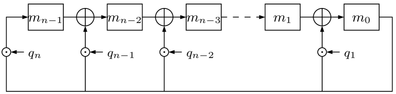
(a) Galois LFSR

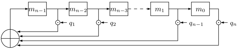
(b) Fibonacci LFSR

Figure 2: Implementation of Galois and Fibonacci LFSRs with connection polynomial $Q(X)=q_{n}X^{n}+\cdots+q_{1}X+1$

Another special kind of LFSMs is the 3-neighborhood cellular automaton (CA) [11, 15, 16, 3]. These automata are characterized by a tri-diagonal matrix as presented in Figure 3. They are suitable for hardware implementation.

$T_{CA}=\begin{pmatrix}q_{1}&1&&&\\ 1&q_{2}&1&(0)&\\ &\ddots&\ddots&\ddots&\\ &(0)&1&q_{n-1}&1\\ &&&1&q_{n}\end{pmatrix}$

(a) Transition matrix of a CA

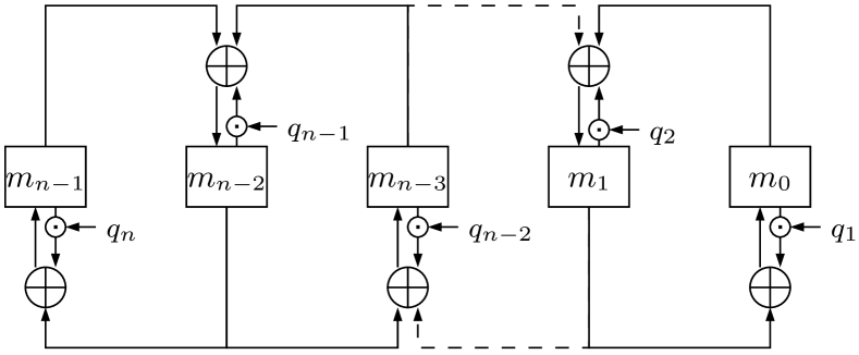
(b) Implementation of a CA

Figure 3: Transition matrix and implementation of a 3-neighborhood Cellular Automaton

To cover numerous kind of automata presented in [3, 17, 16, 18], we introduce Ring LFSRs. The cells which store the state are organized in a cyclic shift register. This corresponds to a transition matrix of a particular form:

Definition III.7

An LFSM ${\mathcal{L}}$ with transition matrix $A$ is called a Ring Linear Feedback Shift Register if $A=(a_{i,j})_{0\leq i,j<n}$ as the following form:

$$\left\{\begin{array}[]{l}a_{i,i+1}=1\text{ for all }0\leq i<n-1\\ a_{n-1,0}=1\end{array}\right.$$

i.e.,

$$A=\begin{pmatrix}&1&&(*)&\\ &&\ddots&&\\ &(*)&&\ddots&\\ &&&&1\\ 1&&&&\\ \end{pmatrix}$$

In particular, Galois and Fibonacci LFSRs are special cases of Ring LFSRs.

We detail here a complete example of these automata. Consider the primitive connection polynomial $Q(X)=X^{8}+X^{6}+X^{5}+X^{3}+1$. Denote ${\mathcal{L}}_{0}$ the associated Galois LFSR, ${\mathcal{L}}_{1}$ the associated Fibonacci LFSR and ${\mathcal{L}}_{2}$ a generic Ring LFSR with connection polynomial $Q(X)$. We present their respective transition matrices $T_{0}$, $T_{1}$ and $T_{2}$ in Figure 4. Figure 5 shows the implementation of ${\mathcal{L}}_{0}$, ${\mathcal{L}}_{1}$ and ${\mathcal{L}}_{2}$ whereas Table I displays the states of these automata during 8 clocks starting from the same initial state.

$T_{0}=\begin{pmatrix}0&1&&&&&&\\ 0&&1&&&(0)&&\\ 1&&&1&&&&\\ 0&&&&1&&&\\ 1&&&&&1&&\\ 1&&(0)&&&&1&\\ 0&&&&&&&1\\ 1&&&&&&&\\ \end{pmatrix}$

(a) Galois LFSR

$T_{1}=\begin{pmatrix}&1&&&&&&\\ &&1&&&(0)&&\\ &&&1&&&&\\ &&&&1&&&\\ &&&&&1&&\\ &&(0)&&&&1&\\ &&&&&&&1\\ 1&0&1&1&0&1&0&0\\ \end{pmatrix}$

(b) Fibonacci LFSR

$T_{2}=\begin{pmatrix}&1&&&&&&\\ &&1&&&(0)&&\\ &&&1&&&&\\ &&&&1&&&1\\ &&&&&1&&\\ &&(0)&&&&1&\\ &&&&&&&1\\ 1&&1&&&&&\\ \end{pmatrix}$

(c) Ring LFSR

Figure 4: Transition matrices of ${\mathcal{L}}_{0}$, ${\mathcal{L}}_{1}$ and ${\mathcal{L}}_{2}$

(a) Galois LFSR ${\mathcal{L}}_{0}$

(b) Fibonacci LFSR ${\mathcal{L}}_{1}$

(c) Ring LFSR ${\mathcal{L}}_{2}$

Figure 5: Three LFSR with connection polynomial $Q(X)=X^{8}+X^{6}+X^{5}+X^{3}+1$

$$\begin{array}[]{|c||c|c|c|}\hline\cr&{\mathcal{L}}_{0}&{\mathcal{L}}_{1}&{\mathcal{L}}_{2}\\ \cline{2-4}\cr Clock&Cells&Cells&Cells\\ &7654321\ 0&7654321\ 0&7654321\ 0\\ \hline\cr\hline\cr 0&\texttt{0000000\ 1}&\texttt{0000000\ 1}&\texttt{0000000\ 1}\\ 1&\texttt{1011010\ 0}&\texttt{1000000\ 0}&\texttt{1000000\ 0}\\ 2&\texttt{0101101\ 0}&\texttt{0100000\ 0}&\texttt{0100100\ 0}\\ 3&\texttt{0010110\ 1}&\texttt{0010000\ 0}&\texttt{0010010\ 0}\\ 4&\texttt{1010001\ 0}&\texttt{1001000\ 0}&\texttt{1001001\ 0}\\ 5&\texttt{0101000\ 1}&\texttt{0100100\ 0}&\texttt{0100000\ 1}\\ 6&\texttt{1001110\ 0}&\texttt{1010010\ 0}&\texttt{1010000\ 0}\\ 7&\texttt{0100111\ 0}&\texttt{0101001\ 0}&\texttt{0101100\ 0}\\ 8&\texttt{0010011\ 1}&\texttt{0010100\ 1}&\texttt{0010110\ 0}\\ \hline\cr\end{array}$$

TABLE I: States of ${\mathcal{L}}_{0}$, ${\mathcal{L}}_{1}$ and ${\mathcal{L}}_{2}$ during 8 clocks.

The reader can see that from the same initial state 00000001 the output sequences are distinct. However, they are all a part of the same $m$-sequence defined by $Q(X)=X^{8}+X^{6}+X^{5}+X^{3}+1$ according to Theorem III.3. In other words there exists three different polynomials $P_{0}(X),P_{1}(X),P_{2}(X)$ of degrees less than 8 such that the sequences generated by ${\mathcal{L}}_{0}$, ${\mathcal{L}}_{1}$ and ${\mathcal{L}}_{2}$ are respectively $P_{0}(X)/Q(X)$, $P_{1}(X)/Q(X)$ and $P_{2}(X)/Q(X)$.

IV Rational representation

In this section, we will introduce a generalization of LFSRs and LFSMs by extending the set of possible coefficients for the transition matrix to rational fractions. This new approach is not only of theoretical interest, but is also an interesting tool for both having a more global view of complex circuits and for constructing more complex circuits from smaller LFSMs with nice properties. Each coefficient of such a matrix is a rational fraction which represents a small LFSM. The inputs and outputs of each small LFSM are thus used as a part of the full automaton.

This new representation allows an easier description of complex circuits with small internal components such as the so-called Windmill generators [4]. These generators are for example used in the stream cipher E0 [5] implemented in the Bluetooth system.

This rational representation leads to a simpler representation of some circuits with multiple outputs at each iteration or of parallelized versions of LFSRs.

This section is organized as follows: we first focus our analysis on LFSMs with a single input and a single output. Then we introduce the notion of transition matrix with rational coefficients. We demonstrate that the automata built using this new representation essentially produce the same sequences than the classical LFSRs. We give a first example based on this new representation to construct a filtered LFSR automaton. We then focus our work on the case of Windmill generators and give a simpler and more compact definition of such LFSRs. We thus discuss the difficulty of implementing such automata which is not so easy in the general case. Finally, we conclude this section with a concrete example. It consists in a generalization of Windmill generators that allows to construct complex circuits from simpler well designed circuits. These simple circuits are building blocks of a bigger automaton which connects the small components in a circular way. The full circuit inherits good internal properties of the smaller components.

IV-A LFSMs with a single input and a single output

As a building block for our representation, we are first interested by an LFSM with a single input bit and a single output bit. In this situation, the matrix $B$ is a $n\times 1$ matrix, with a single 1 in position $i_{0}$. Likewise, $C$ is a $1\times n$ matrix, with a single 1 in position $j_{0}$.

Set $A^{\prime}=\operatorname{adj}(I-XA)=(A^{\prime}_{i,j}(X))$, where the coefficients $A^{\prime}_{i,j}(X)$ are polynomials, and $Q(X)=\det(I-X.A)$. We can derive from Theorem III.3, the following relation between the input series $U^{(t)}$ and the output series $V^{(t)}$:

$$V^{(t)}=\frac{X}{Q(X)}CA^{\prime}BU^{(t)}+\frac{1}{Q(X)}CA^{\prime}m^{(t)}$$

Note that $CA^{\prime}B=A^{\prime}_{j_{0},i_{0}}(X)$ is a polynomial, and $P^{(t)}(X)=CA^{\prime}m^{(t)}$ is also a polynomial. Setting $R(X)=XA^{\prime}_{i_{0},j_{0}}(X)$, we can rewrite the previous formula

$$V^{(t)}=\frac{R(X)}{Q(X)}U^{(t)}+\frac{P^{(t)}(X)}{Q(X)}$$

Note that $R(X)$ is independent of the internal state $m^{(t)}$ of the LFSM, and $\frac{P^{(t)}(X)}{Q(X)}$ is uniquely determined by the internal state $m^{(t)}$ of the LFSM.

So up to initial internal values of such LFSM, we can consider that it performs the multiplication of the input by the rational series $R(X)/Q(X)$ (note that, since $Q(X)=\det(I-X.A)$, we have $Q(0)=1\neq 0$).

Conversely, for a given rational power series $R(X)/Q(X)$, $Q(0)\neq 0$, it is possible to construct many LFSMs which perform the multiplication by $R(X)/Q(X)$.

As an example of such LFSMs, we give in Figure 6 an LFSM with one input and one output which performs the multiplication by $R(X)/Q(X)$ called in the rest of this paper a Galois vane (in reference to a Galois LFSR and a vane of a windmill generator).

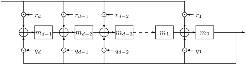
Figure 6: Implementation of a division/multiplication circuit

The matrix description of this LFSM is:

$$A=\begin{pmatrix}q_{1}&1&&&\\ q_{2}&&1&(0)&\\ \vdots&&(0)&\ddots&\\ q_{d-1}&&&&1\\ q_{d}&0&0&\cdots&0\end{pmatrix},B=\begin{pmatrix}r_{1}\\ r_{2}\\ \vdots\\ r_{d-1}\\ r_{d}\end{pmatrix}$$

and $C=(1,0,\ldots,0)$.

it will be interesting to use some multiplication/division circuits which are not performed by a Galois vane. As an example, we consider the ring LFSR described in Figure 5. The connection polynomial is $Q(X)=X^{8}+X^{6}+X^{5}+X^{3}+1$. Let $T^{\prime}=\operatorname{adj}{I-XT_{2}}$, we have $T^{\prime}_{1,1}=X^{6}+X^{3}+1$ and $T^{\prime}_{4,3}=X^{7}+X^{5}+X^{4}+X^{2}$. For ${}^{t}B=C=(1,0,...,0)$, this ring LFSR performs the multiplication by $(X^{6}+X^{3}+1)/(X^{8}+X^{6}+X^{5}+X^{3}+1)$. For ${}^{t}B=(0,0,0,1,0,0,0,0)$ and $C=(0,0,1,0,...,0)$, it performs the multiplication by $(X^{7}+X^{5}+X^{4}+X^{2})/(X^{8}+X^{6}+X^{5}+X^{3}+1)$. For these two examples, the circuit is simpler than the equivalent one obtained by the Galois vane.

IV-B Rational Linear Machines

Now, we want to use multiplications by rational power series $R(X)/Q(X)$, with $Q(0)\neq 0$, as internal building blocks in order to construct bigger LFSMs.

Recall that we denote by ${\mathcal{Q}}$ the ring of rational power series, that is $\{P(X)/Q(X)\in{\mathbb{F}}_{2}[[X]]\mid P(X),Q(X)\in{\mathbb{F}}_{2}[X],Q(0)\neq 0\}$.

Definition IV.1

A Rational Linear Machine (RLM) ${\mathcal{L}}$ with $k$-bit input, $\ell$-bit output and length $n$ over ${\mathcal{Q}}$ is a triplet of matrices $(A,B,C)$ over ${\mathcal{Q}}$, of respective sizes $n\times n$, $n\times k$, $\ell\times n$. Given the current state vector $(m^{(t)},c^{(t)})\in{\mathcal{M}}_{n,1}({\mathbb{F}}_{2})\times{\mathcal{M}}_{n,1}({\mathcal{Q}})$ and input vector $u^{(t)}\in{\mathcal{M}}_{k,1}({\mathbb{F}}_{2})$. The next state vector $(m^{(t+1)},c^{(t+1)})$ and the present output vector $v^{(t)}\in{\mathcal{M}}_{\ell,1}({\mathbb{F}}_{2})$ are expressed as:

$$\left\{\begin{array}[]{rcl}m^{(t+1)}&=&Am^{(t)}+c^{(t)}+Bu^{(t)}\bmod X\\ c^{(t+1)}&=&Am^{(t)}+c^{(t)}+Bu^{(t)}\operatorname{div}X\\ v^{(t)}&=&Cm^{(t)}\end{array}\right.$$

where $P(X)\operatorname{div}X=\frac{P(X)-(P(X)\bmod X)}{X}$.

As previously we are able to describe the output sequences:

Theorem IV.2

Let ${\mathcal{L}}=(A,B,C)$ a RLM. The vector $M^{(t)}$ satisfy the relation:

$$M^{(t)}=(I-XA)^{-1}\left(m^{(t)}+Xc^{(t)}+XBU^{(t)}\right)$$

Proof:

With the previous notations we have the following relations:

$$M^{(t+1)} = AM^{(t)}+c^{(t)}+BU^{(t)}$$ (6)

$$M^{(t)} = XM^{(t+1)}+m^{(t)}$$ (7)

Equation 6 is by Definition IV.1. Equation 7 comes from the Definition of $M^{(t)}$. It leads to the following relation:

$$(I-XA)M^{(t_{0})}=m^{(t_{0})}+Xc^{(t_{0})}+XBU^{(t)}$$

Note that $(I-XA)$ is invertible in ${\mathcal{M}}_{n}({\mathcal{Q}})$. This leads to $M^{(t_{0})}=(I-XA)^{-1}(m^{(t_{0})}+Xc^{(t_{0})}+XBU^{(t)})$ in ${\mathcal{Q}}$. ∎

IV-C Rational Linear Finite State Machines

In order to focus the attention on some applications, and for a better understanding of the significance of Theorem IV.2, we focus in this Section on the study of RLM with no input. Moreover, we will try to limit the domain of the “carries” register $c$ in order to ensure that the machine is a finite state machine. We suppose in the sequel that $B=0$, i.e. there is no input.

In order to restrict RLM to finite state machines, we have to look at the evolution of “internal memories” $c^{(t)}$ in more details. Let $A_{i,j}=P_{i,j}(X)/Q_{i,j}(X)$ be the expression of a coefficient of the matrix $A$ as a quotient of two polynomials. For a fixed row $i$ we can compute the polynomial $Q_{i}(X)=\mbox{lcm}(Q_{i,1}(X),\dots,Q_{i,n}(X))$. So we can normalize the rational representations as follows: $A_{i,j}=R_{i,j}(X)/Q_{i}(X)$. For each row $i$ we define the following finite subset of ${\mathcal{Q}}$: $W_{i}=\{R(X)/Q_{i}(X)\>|\>\deg(R(X))<\max_{j}(\deg(R_{i,j}(X)))\}$. Finally we define $W=\prod_{i=1}^{n}W_{i}\subset{\mathcal{Q}}^{n}$. Note that $W$ is a finite set. The following proposition shows that it is a “reasonable” set for the values of the internal memories;

Proposition IV.3

Suppose that at time $t_{0}$, $c^{(t_{0})}$ is in $W$, then for any $t\geq t_{0}$, $c^{(t)}$ is in $W$.

Proof:

Let $\mu^{(t+1)}=Am^{(t)}+c^{(t)}$. From the definition of a RLM, we have $m^{(t+1)}=\mu^{(t+1)}\bmod X$ and $c^{(t+1)}=\mu^{(t+1)}\operatorname{div}X$.

If we consider the $i$-th row of $A$, we obtain $\mu^{(t+1)}_{i}=\sum_{j=1}^{n}m_{j}^{(t)}R_{i,j}(X)/Q_{i}(X)+c^{(t)}_{i}$. So under the condition $c^{(t)}_{i}\in W_{i}$, $\mu^{(t+1)}_{i}$ can be expressed as a rational fraction of the form $R^{\prime}_{i}/Q_{i}$ and $\deg(R^{\prime}_{i})\leq\max_{j}(\deg(R_{i,j}(X))$, this implies $c^{(t+1)}\in W_{i}$. ∎

Following this result we want to limit the “carries” part of a RLM to the domain $W$. So we give the following definition for RLFSMs, which is a true finite state machine.

Definition IV.4

A Rational Linear Finite State Machine (RLFSM) with $\ell$-bit output and length $n$ over ${\mathcal{Q}}$ is a finite state automaton defined by a pair $(A,C)$ of matrices over ${\mathcal{Q}}$ , with respective sizes $n\times n$ and $\ell\times n$. The space of states of this automaton is ${\mathbb{F}}_{2}^{n}\times W$ where $W$ is defined from $A$ as previously explained, the transition and extraction functions at time $t$ are defined by: if the automaton is in the state $(m^{(t)},c^{(t)})$ at time $t$ and $v^{(t)}$ is the output at time $t$, then

$$\left\{\begin{array}[]{rcl}m^{(t+1)}&=&Am^{(t)}+c^{(t)}\bmod X\\ c^{(t+1)}&=&Am^{(t)}+c^{(t)}\operatorname{div}X\\ v^{(t)}&=&Cm^{(t)}\end{array}\right.$$

Now, we want to characterize in more details the output of a RLFSM. Set $G(X)=\prod_{i=1}^{n}Q_{i}(X)$. We have $A=\frac{1}{G(X)}A^{\prime}$, where $A^{\prime}$ is a matrix with polynomial coefficients.

From the definition of $A^{\prime}$, we have $\det(I-XA)=\frac{1}{G(X)^{n}}\det(G(X)I-XA^{\prime})$ where $T(X)=\det(G(X)I-XA^{\prime})$ is a polynomial. So we obtain $(I-XA)^{-1}=\frac{G(X)^{n}}{T(X)}\operatorname{adj}(I-XA^{\prime})$, where $\operatorname{adj}(I-XA^{\prime})$ is a matrix with polynomial coefficients.

We can easily deduce the rational form of the output of a RLFSM

Proposition IV.5

Let ${{\mathcal{L}}}$ be a RLFSM defined by a transition matrix $A$ and any output matrix $C$. Set $T(X)=\det(G(X)(I-XA))$. The output sequences $V^{(t)}_{i}$ are rational power series of the form $P_{i}(X)/T(X)$.

Proof:

This result comes from the formula

$$\begin{array}[]{rcl}M^{(t)}&=&(I-XA)^{-1}(m^{(t)}+Xc^{(t)})\\ &=&\frac{G(X)^{n}}{T(X)}\operatorname{adj}(I-XA^{\prime})(m^{(t)}+Xc^{(t)}).\end{array}$$

Indeed, the denominators of the coefficients of the matrix $(I-XA)^{-1}$ are some divisors of $T(X)$, $m^{(t)}$ is a binary vector and $c^{(t)}\in W$ is such that $G(X)^{n}Xc^{(t)}$ is a polynomial vector. ∎

Note that the rational power series $P_{i}(X)/T(X)$ are a priori not irreducible. In practice, the numerator is often the polynomial $Q(X)$ such that $Q(X)/P(X)$ is the irreducible rational representation of $\det(I-XA)$.

IV-D A first example

We consider a filtered LFSR in Galois mode of size $n=12$ with connection polynomial $Q(X)=1+X^{5}+X^{6}+X^{7}+X^{9}+X^{11}+X^{12}$, filtered by a Boolean function in cells $m_{0}$, $m_{5}$, $m_{7}$ and $m_{9}$.

If we are interested only on the filtered output bits, this LFSR can be described by a RLFSM with the matrix

$$A^{\prime}=\begin{pmatrix}X^{4}&X^{4}&0&0\\ 1+X&0&X&0\\ X&0&0&X\\ X+X^{2}&0&0&0\end{pmatrix}$$

This matrix leads to a new representation of this RLFSM:

Let $B=(I-XA^{\prime})^{-1}$, and $Q(X)=\det(I-XA^{\prime})=X^{12}+X^{11}+X^{9}+X^{7}+X^{6}+X^{5}+1$. Then the value of $B$ is

$$B=\frac{1}{Q(X)}\begin{pmatrix}P_{1,1}&P_{1,2}&P_{1,3}&P_{1,4}\\ P_{2,1}&P_{2,2}&P_{2,3}&P_{2,4}\\ P_{3,1}&P_{3,2}&P_{3,3}&P_{3,4}\\ P_{4,1}&P_{4,2}&P_{4,3}&P_{4,4}\\ \end{pmatrix}$$

with $P_{1,1}(X)=1$, $P_{1,2}(X)=X^{5}$, $P_{1,3}(X)=X^{7}$, $P_{1,2}(X)=X^{9}$, $P_{2,1}(X)=X^{7}+X^{6}+X^{4}+X^{2}+X$, $P_{2,2}(X)=X^{5}+1$, $P_{2,3}(X)=X^{7}+X^{6}+X^{5}+1$, $P_{2,4}(X)=X^{9}+X^{8}+X^{7}+X^{2}$, $P_{3,1}(X)=X^{5}+X^{4}+X^{2}$, $P_{3,2}(X)=X^{10}+X^{9}+X^{7}$, $P_{3,3}(X)=X^{7}+X^{6}+X^{5}+1$, $P_{3,4}(X)=X^{9}+X^{8}+X^{7}+X^{2}$, $P_{4,1}(X)=X^{3}+X^{2}$, $P_{4,2}(X)=X^{8}+X^{7}$, $P_{4,3}(X)=X^{10}+X^{9}$ and
$P_{4,4}(X)=X^{9}+X^{7}+X^{6}+X^{5}+1$.

If we denote by $(a_{0},\ldots,a_{12})$ the initial state at time $t=0$ of the binary LFSR, then, the initial state of our RLFSM is $m^{(0)}=(a_{0},a_{5},a_{7},a_{9})$ and $c^{(0)})=(a_{1}+a_{2}X+a_{3}X^{2}+a_{4}X^{3},a_{6},a_{8},a_{10}+a_{11}X)$ and the sequences in output are
$\frac{a_{0}P_{1,1}(X)+a_{5}P_{1,2}(X)+a_{7}P_{1,3}(X)+a_{9}P_{1,4}(X)}{Q(X)}$
a +$\frac{(a_{1}+a_{2}X+a_{3}X^{2}+a_{4}X^{3})X}{Q(X)},$
$\frac{a_{0}P_{2,1}(X)+a_{5}P_{2,2}(X)+a_{7}P_{2,3}(X)+a_{9}P_{2,4}(X)+a_{6}X}{Q(X)},$
$\frac{a_{0}P_{3,1}(X)+a_{5}P_{3,2}(X)+a_{7}P_{3,3}(X)+a_{9}P_{3,4}(X)+a_{8}X}{Q(X)},$
$\frac{a_{0}P_{4,1}(X)+a_{5}P_{4,2}(X)+a_{7}P_{4,3}(X)+a_{9}P_{4,4}(X)+(a_{10}+a_{11})X}{Q(X)}$.

IV-E Application to windmill LFSRs

Windmill LFSRs can be defined as LFSMs with no input and several outputs. They have been introduced in [4] as a cyclic cascade connection of $v\geq 1$ LFSMs. Each of these LFSMs is called a vane of the windmill. The classical representation of those LFSMs is the Fibonacci one. However, in the rest of this section, we will show them using the equivalent Galois representation because it is more suitable for a better understanding. Windmill LFSRs are characterized by their feedback and feedforward connections. These feedback and feedforward connections are identical for all vanes, but the lengths of the LFSMs may be different as they can be shifted in different LFSMs. Figure 6 presents a generic vane in Galois mode.

Windmill LFSRs were introduced to achieve parallel generation of sequences. Consider a sequence $S=(s_{n})_{n\in{\mathbb{N}}}$. While a classical automaton outputs $s_{0}$ at the first clock, $s_{1}$ at the second, and so on, a parallel automaton outputs $v$ bits at each clock: $(s_{0},s_{1},\ldots,s_{v-1})$ at the first clock, $(s_{v},\ldots,s_{2v-1})$ at the second, etc. More precisely a parallel automaton has $v$ outputs and products the sequences $S^{i}:=(s_{nv+i})_{n\in{\mathbb{N}}}$ where $0\leq i<v$. Note that our study focus on characterizing the sequences $S^{i}$ and not the reconstructed sequence $S$.

Consider the windmill presented in Figure 7 which is the one used in the stream cipher E0 [5]. It is constituted of one vane of length $7$ and three identical vanes of length $6$. No feedback connection appears. Feedforward connections appear, for example from cell $m_{13}$ to cells $m_{12}$, $m_{10}$, $m_{9}$ and $m_{7}$.

Figure 7: A windmill with only feedforward connections.

Until now, only windmill LFSRs with a single vane repeated several times have been studied. We generalize this definition allowing different vanes in a windmill. We also give a new description of this windmill which will be more compact. More precisely, using the example, we want to consider output sequences of cells $m_{0}$, $m_{7}$, $m_{13}$ and $m_{19}$, and characterize each vane by a polynomial. This leads to the interpretation presented in Figure 8.

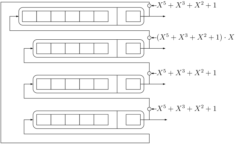
Figure 8: A windmill in rational representation.

With this definition the LFSM described in Figure 8 as the following transition matrix:

$$(X^{5}+X^{3}+X^{2}+1)\cdot\begin{pmatrix}0&X&0&0\\ 0&0&1&0\\ 0&0&0&1\\ 1&0&0&0\end{pmatrix}$$

We give in Table II the values of $m^{(t)}$ and $c^{(t)}$ during 8 clocks.

$$\begin{array}[]{|c||c|c|c|c||c|c|c|c|}\hline\cr Clock&m_{0}^{(t)}&m_{1}^{(t)}&m_{2}^{(t)}&m_{3}^{(t)}&c_{0}^{(t)}&c_{1}^{(t)}&c_{2}^{\prime(t)}&c_{3}^{(t)}\\ \hline\cr\hline\cr 0&1&0&0&0&0&0&0&0\\ 1&0&0&0&1&0&0&0&X^{4}+X^{2}+X\\ 2&0&0&1&0&0&0&X^{4}+X^{2}+X&X^{3}+X+1\\ 3&0&1&0&1&0&X^{4}+X^{2}+X&X^{3}+X+1&X^{2}+1\\ 4&0&0&0&1&X^{5}+X^{3}+X^{2}+1&X^{3}+X+1&X^{4}+X+1&X\\ 5&1&1&0&0&X^{4}+X^{2}+X&X^{2}+1&X^{4}+X^{3}+X^{2}+X+1&1\\ 6&0&1&1&0&X^{5}+X^{2}+X&X&X^{3}+X^{2}+X+1&X^{4}+X^{2}+X\\ 7&0&1&1&0&X^{5}+X^{4}+X^{3}+X^{2}+X&X^{4}+X^{2}+X+1&X^{2}+X+1&X^{3}+X+1\\ 8&0&0&1&1&X^{5}+X^{4}+X&X^{4}+X^{3}+X^{2}+1&X+1&X^{2}+1\\ \hline\cr\end{array}$$

TABLE II: States of Figure 8 during 8 clocks.

According to Definition IV.4, windmills as introduced by Smeets and Chambers [4] agree with the following definition:

Definition IV.6

A windmill LFSR with polynomials $\alpha(X),\beta(X)$ with $\beta(0)\not=0$ and $v$ vanes is an LFSR of length $v$ with matrix $A$ over ${\mathbb{F}}_{2}[[X]]$ of the form:

$$\begin{pmatrix}0&\frac{\alpha(X)}{\beta(X)}X^{i_{0}}&&(0)\\ \vdots&\ddots&\ddots&\\ 0&(0)&\ddots&\frac{\alpha(X)}{\beta(X)}X^{i_{v-2}}\\ \frac{\alpha(X)}{\beta(X)}X^{i_{v-1}}&0&\dots&0\\ \end{pmatrix}$$

where $0\leq i_{0},\ldots,i_{v-1}$.

With this representation each row represents a vane of the windmill. In particular, as described in the following section the length of the vane $j$ is equal to $\max(\deg(\alpha(X)X^{i_{j}}),\deg(\beta(X)))$.

By a straightforward calculus, we obtain $\det(I-XA)=X^{n}\left(\alpha(X)/\beta(X)\right)^{v}+1$, where $n=i_{0}+\cdots+i_{v-1}$. Set $Q(X)=X^{n}\alpha(X)^{v}+\beta(X)^{v}$, it becomes $\det(I-XA)=Q(X)/\beta(X)^{v}$. The sequences $M_{i}^{(t)}$ observed in the output of this RLFSM are of the form $P_{i}(X)/Q(X)$. The main result on windmill generators (c.f. [4]) is the fact that there exists a permutation $\sigma$ of $\{0,\ldots,v-1\}$ such that the series $S(X)=\sum_{t}(\sum_{i=0}^{v-1}m_{i}(t)X^{\sigma(i)})X^{vt}$ is a rational power series of the form $P(X)/Q(X^{v})$. In other words, a windmill generator is able to output in parallel at each iteration $v$ consecutive values of a rational power series. The most interesting case is the one where $Q(X^{v})$ is a primitive polynomial. Such windmill generators are used in the specification of the pseudo-random generator E0 included in the specifications of Bluetooth [5].

Our polynomial approach gives a more synthetic point of view on these windmill generators. In particular, it shows that the windmill properties (i.e. the parallel generation of a given $m$-sequence) is independent of the implementation of the vanes. This implementation can be made with Fibonacci vanes as in the original version, or with Galois vanes as presented previously or with ring vanes with better diffusion delay as we will see in the next section.

IV-F Implementation of RLFSMs

In our previous examples, the starting point was a binary circuit, or a RLFSM with a particular structure for its matrix. The converse problem is “how to construct an efficient implementation from a given transition matrix $A$ of a RLFSM”. We will show on two examples that this task is not so easy.

IV-F1 A first example

Consider the RLFSM ${\mathcal{L}}^{1}$ defined by the following transition matrix:

$$A=\begin{pmatrix}\frac{X^{2}}{X^{3}+1}&\frac{X}{X^{2}+X+1}\\ 1&0\end{pmatrix}$$

We compute $(I-XA)^{-1}$ to characterize the output sequences:

$$(I-XA)^{-1}=\begin{pmatrix}\frac{X^{3}+1}{X^{4}+X^{3}+1}&\frac{X^{3}+X^{2}}{X^{4}+X^{3}+1}\\ \frac{X^{4}+X}{X^{4}+X^{3}+1}&\frac{1}{X^{4}+X^{3}+1}\end{pmatrix}$$

Figure 9 presents an implementation of this automaton built upon three LFSMs. One for each nonzero coefficient in $A$. These LFSMs are built using a Galois vane architecture as presented in Figure 6.

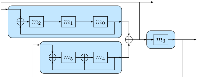
Figure 9: First implementation of ${\mathcal{L}}^{1}$.

Note that, according to the notation of Figure 9, ${\mathcal{L}}^{1}$ can be expressed as the LFSM $(A^{\prime},0,C^{\prime})$ with:

$$A^{\prime}=\begin{pmatrix}0&1&0&0&0&0\\ 0&0&1&0&0&0\\ 0&0&0&0&1&0\\ 1&0&0&0&1&0\\ 0&0&0&0&1&1\\ 0&0&0&1&1&0\end{pmatrix},\ C^{\prime}=\begin{pmatrix}1&0&0&0&1&0\\ 0&0&0&1&0&0\end{pmatrix}$$

In particular, we have the following relations according to Theorem III.3:

$$V^{(t)}=\frac{1}{X^{4}+X^{3}+1}\quad\times\\ \begin{pmatrix}1&X&X^{2}&X^{3}+X^{2}&X+1&X^{2}+X\\ X&X^{2}&X^{3}&1&X^{2}+X&X^{3}+X^{2}\end{pmatrix}m^{(t)}$$

This implementation is not optimal because it requires seven memories cells while four are enough (it outputs sequences of the form $P(X)/(X^{4}+X^{3}+1)$ with $\deg P(X)<3$). In particular, $\det(I-XA^{\prime})=X^{6}+X^{3}+X^{2}+X+1$, i.e., this automaton could output $m$-sequences of the form $P(X)/(X^{6}+X^{3}+X^{2}+X+1)$ using a different matrix $C^{\prime}$ because $X^{6}+X^{3}+X^{2}+X+1$ is primitive.

A better implementation is given considering one LFSM per line. To do so, note that $\frac{X}{X^{2}+X+1}=\frac{X^{2}+X}{X^{3}+1}$. This leads to the implementation presented in Figure 10.

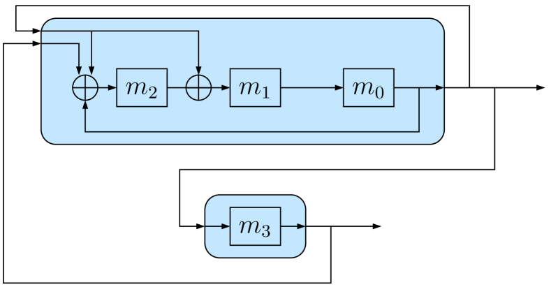
Figure 10: Second implementation of ${\mathcal{L}}^{1}$.

As previously this leads to the relation:

$$V^{(t)}=\\ \begin{pmatrix}\frac{1}{X^{4}+X^{3}+1}&\frac{X}{X^{4}+X^{3}+1}&\frac{X^{2}}{X^{4}+X^{3}+1}&\frac{X^{3}+X^{2}}{X^{4}+X^{3}+1}\\ \frac{X}{X^{4}+X^{3}+1}&\frac{X^{2}}{X^{4}+X^{3}+1}&\frac{X^{3}}{X^{4}+X^{3}+1}&\frac{1}{X^{4}+X^{3}+1}\end{pmatrix}m^{(t)}.$$

IV-F2 Second example

Consider the RLFSM ${\mathcal{L}}^{2}$ defined by the following transition matrix:

$$A=\begin{pmatrix}\frac{X+1}{X^{3}+X+1}&\frac{X}{X^{2}+X+1}&0\\ X^{3}+X^{2}&X^{2}&1\\ 0&\frac{X+1}{X^{2}+X+1}&0\end{pmatrix}$$

Figure 11 presents an implementation of this automaton built upon six LFSMs. One for each nonzero coefficient in $A$. These LFSMs are built using a Galois vane architecture as presented in Figure 6.

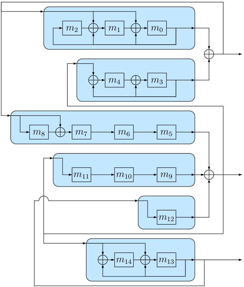
Figure 11: First implementation of ${\mathcal{L}}^{2}$.

Note that, according to the notation of Figure 11, ${\mathcal{L}}^{2}$ can be expressed as the LFSM $(A^{\prime},0,C^{\prime})$ with:

$$A^{\prime}=\left(\begin{array}[]{ccccccccccccccc}0&1&0&1&0&0&0&0&0&0&0&0&0&0&0\\ 1&0&1&1&0&0&0&0&0&0&0&0&0&0&0\\ 1&0&0&0&0&0&0&0&0&0&0&0&0&0&0\\ 0&0&0&1&1&1&0&0&0&1&0&0&1&0&0\\ 0&0&0&1&0&1&0&0&0&1&0&0&1&0&0\\ 0&0&0&0&0&0&1&0&0&0&0&0&0&0&0\\ 0&0&0&0&0&0&0&1&0&0&0&0&0&0&0\\ 1&0&0&1&0&0&0&0&1&0&0&0&0&0&0\\ 1&0&0&1&0&0&0&0&0&0&0&0&0&0&0\\ 0&0&0&0&0&0&0&0&0&0&1&0&0&0&0\\ 0&0&0&0&0&0&0&0&0&0&0&1&0&0&0\\ 0&0&0&0&0&1&0&0&0&1&0&0&1&0&0\\ 0&0&0&0&0&0&0&0&0&0&0&0&0&1&0\\ 0&0&0&0&0&1&0&0&0&1&0&0&1&1&1\\ 0&0&0&0&0&1&0&0&0&1&0&0&1&1&0\end{array}\right)$$

and

$$C^{\prime}=\left(\begin{array}[]{ccccccccccccccc}1&0&0&1&0&0&0&0&0&0&0&0&0&0&0\\ 0&0&0&0&0&1&0&0&0&1&0&0&1&0&0\\ 0&0&0&0&0&0&0&0&0&0&0&0&0&1&0\end{array}\right)$$

This implementation is not optimal because it requires fifteen memories cells while nine are enough because ${\deg(\det(I-XA))}=9$. In particular, $\deg(\det(I-XA^{\prime}))=11$.

A better implementation is given considering one LFSM per line. This leads to the implementation presented in Figure 12.

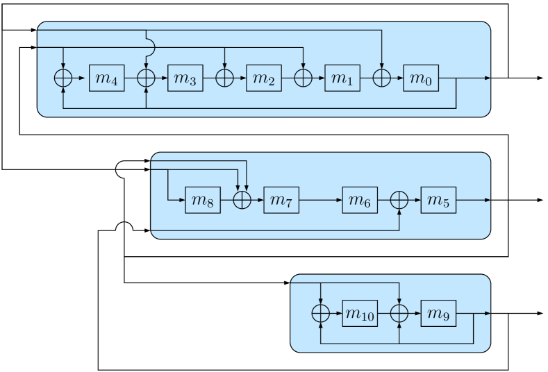
Figure 12: Second implementation of ${\mathcal{L}}^{2}$.

This implementation is still not optimum because it requires eleven memory cells. This comes from the fact that in the matrix $A$, two terms with identical denominator appears in the same column: $\frac{X}{X^{2}+X+1}$ and $\frac{X+1}{X^{2}+X+1}$. More precisely, $\det(I-XA^{\prime})=(X+1)(X^{2}+X+1)(X^{8}+X^{7}+X^{5}+X^{4}+X^{3}+X^{2}+1)$. Thus, the automaton could be implemented using the nine cells equivalent with the polynomial $(X+1)(X^{8}+X^{7}+X^{5}+X^{4}+X^{3}+X^{2}+1)$ which is reducible and thus not primitive whereas the last factor disappears inside the automaton itself.

IV-G A practical example of application

The rational representation is a theoretical tool that provides a global view on the LFSRs design, as seen for the case of windmill generators. However, previous examples have shown that starting from a circuit under rational representation to obtain an optimal implementation is not a simple task.

In the example given here, we generalize the windmills generators through particular series circuits. We limit our study with an example built on 3 circuits but the generalization of this method is straightforward.

Let $A_{1}(X)=P_{1}(X)/Q_{1}(X)$, $A_{2}(X)=P_{2}(X)/Q_{2}(X)$ and $A_{3}(X)=P_{3}(X)/Q_{3}(X)$ be 3 elements of ${\mathcal{Q}}$. We consider the rational LFSR with transition matrix

$$T=\left(\begin{array}[]{ccc}0&A_{1}&0\\ 0&0&A_{2}\\ A_{3}&0&0\\ \end{array}\right).$$

We have $\det(I-XT)=1-X^{3}A_{1}A_{2}A_{3}=Q(X)/(Q_{1}(X)Q_{2}(X)Q_{3}(X))$ with $Q(X)=Q_{1}(X)Q_{2}(X)Q_{3}(X)+X^{3}Q_{1}(X)P_{1}(X)P_{2}(X)P_{3}(X)$. The associated automaton computes rational series of the form $P(X)/Q(X)$.

Following the examples introduced in Figure 5 and in Section IV-A, we choose $A_{1}(X)=A_{2}(X)=(X^{6}+X^{3}+1)/(X^{8}+X^{6}+X^{5}+X^{3}+1)$ and $A_{3}(X)=(X^{7}+X^{5}+X^{4}+X^{2})/(X^{8}+X^{6}+X^{5}+X^{3}+1)$. The connection polynomial (i.e. the numerator of $\det(I-XT)$) is $Q(X)=X^{24}+X^{21}+X^{16}+X^{9}+X^{7}+X^{3}+1$. This polynomial is primitive, so the automaton will produce $m$-sequences.

For a practical implementation, we can replace the Galois vanes associated to $A_{1}(X)$, $A_{2}(X)$ and $A_{3}(X)$ by the ring vanes presented in Section IV-A.

This leads to a classical binary LFSR with transition matrix

$$T_{r}=\left(\begin{array}[]{ccc}T_{2}&0&E_{1,4}\\ E_{1,1}&T_{2}&0\\ 0&E_{3,1}&T_{2}\\ \end{array}\right).$$

Where $T_{2}$ is the $8\times 8$ matrix of the ring LFSR given in Figure 4 and where $E_{i,j}$ is the $8\times 8$ matrix with only one 1 in position $(i,j)$. The matrices $E_{i,j}$ represent the connections between the 3 circuits. For example, the matrix $E_{1,4}$ corresponds to the input 1 of the first ring LFSR and the output 4 of the third LFSR.

Note that $\det(I-XT_{r})=Q(X)=X^{24}+X^{21}+X^{16}+X^{9}+X^{7}+X^{3}+1$.

Suppose now that we prefer an implementation with Galois vanes as internal blocks. The matrix of the Galois vane is the matrix $T_{0}$ given in Figure 4. The multiplication by $A_{1}(X)$ is performed using ${}^{t}B_{1}=(1,0,0,1,0,0,1,0)$ in input and $C_{1}=(1,0,0,0,0,0,0,0)$ for output. In the same way, we obtain $B_{2}=B_{1}$, ${}^{t}B_{3}=(0,0,1,0,1,1,0,1)$ and $C_{2}=C_{3}=C_{1}$. So the equivalent binary circuit is then

$$T_{g}=\left(\begin{array}[]{ccc}T_{0}&0&B_{1}C_{3}\\ B_{2}C_{1}&T_{0}&0\\ 0&B_{3}C_{2}&T_{0}\\ \end{array}\right).$$

As we will see in the next section the automaton corresponding to the matrix $T_{r}$ has many nice properties compared to the classical ones obtained from the Galois LFSR. In particular, it needs 9 connections compared to 19 for the second one.

This example shows that the rational representation allows to separate the global design of the automaton from the choices of the hardware (or software) implementation.

The method presented in this example can be directly generalized to all Windmill generators and potentially leads to better practical implementations.

V Design of efficient LFSRs for both hardware and software cryptographic applications

In this section, we specialize our work on autonomous LFSMs, in particular on LFSRs and their dedicated use for cryptographic applications.

A general purpose of cryptography is to design primitives that are both efficient in hardware and software because such primitives must run on all possible supports, from RFID tags to super-calculators. Thus, cryptographers must keep in mind, when they design cryptosystems, the very wide range of targets on which cryptosystems must be rapid and efficient. As proof, the Rijndael algorithm chosen as the AES [19] in 2001 was one of the more efficient algorithm in hardware and in software among the finalists of the AES competition.

Thus, designing well-chosen dedicated LFSMs efficient both in hardware and in software has direct consequences on the celerity of the cryptosystems which use such primitives as building blocks. Among cryptographic primitives that use LFSMs, we could cite the most famous case: the stream ciphers. Many stream ciphers - such as E0 [5], SNOW [7] or the finalists SOSEMANUK [20] and Grain v1 [21] of the eStream project [22] - filter the content of one or many LFSMs to output pseudo-random bits. LFSMs could also be used as diffusion layer of a block cipher as proposed in [23]. More recently, in [24], a particular LFSM combined with two NLFSRs (Non-Linear Feedback Shift Registers) has been proposed at CHES 2010 as the building block of a lightweight hash function named Quark. Well designing LFSMs with good criteria is therefore crucial for symmetric key cryptography.

In this section, we first introduce the required design criteria that must be fulfilled by an LFSM when used in cryptographic applications. We then extend the traditional concept of diffusion (well-known in the block cipher context) to the case of LFSMs. This leads to define a new criterion for good LFSMs choices for cryptographic applications which is defined as the counterpart of the Shannon diffusion concept [25].

Then, we present previous works on LFSMs for hardware and software cryptographic applications. These automata have been widely studied [1, 2, 4, 10, 26, 6] and practical constructions have emerged. We finally propose an efficient construction dedicated to hardware and a second one dedicated to software. This software construction is also efficient in hardware.

V-A Design criteria

We focus our design analysis on two important properties. The first one characterizes the kind of sequences that are required for cryptographic applications whereas the second one tries to formalize the notion of diffusion delay in the context of LFSRs.

V-A1 $m$-sequences

As introduced in Section II, $m$-sequences are particular linear recurring sequences with good properties [1, 10]. For example, we give some properties for $m$-sequences of degree $n$ over ${\mathbb{F}}_{2}$:

• an $m$-sequence is balanced: the number of $1$ is one greater than the number of $0$ (considering one period).

• an $m$-sequence has the run property: a run is a sub-sequence of $1$ or $0$ followed and followed by 0 or 1. Half of the runs are of length $1$, a quarter of length $2$, an eighth of length $3$, etc. up to the 1-run of length $n$.

• an $m$-sequence is a punctured De Bruijn sequence.

• an $m$-sequence has the (ideal) two-level autocorrelation function where the autocorrelation function for a binary sequence $a$ is defined as $C_{a}(\tau)=\sum_{i=0}^{N-1}(-1)^{a_{i+\tau}+a_{i}}$ where $N$ is the period of the sequence. This function verifies for a $m$-sequence: $C_{\tau}=N$ if $\tau=0\mod N$ and $C_{\tau}=K$ if $\tau\neq 0\mod N$ (where $K$ is a constant equal to $-1$ if $N$ is odd and to 0 is $N$ even).

• an $m$-sequence has maximum period: an $m$-sequence verifying a linear relation of degree $n$ has a period of $2^{n}-1$.

In the sequel, we are specially interested in LFSMs having a primitive connection polynomial and producing $m$-sequence which are the ones classically used in cryptography. In particular, all our examples satisfy this condition. However, most of the results remains true without this hypothesis.

V-A2 Diffusion delay

The concept of diffusion for a cipher was introduced by C. Shannon in [25] as the dissipating effect of the redundancy of the statistical structure of a message $M$. This concept is directly linked with the Avalanche effect defined by H. Feistel in [27] which is a desirable property of cryptographic algorithms, typically block ciphers and cryptographic hash functions. The Avalanche effect means that if an input is changed slightly, the corresponding output must change significantly. In the case of block ciphers, such a small change in either the key or the plaintext should cause a drastic change in the ciphertext.

Two precise notions could be directly derived: the strict avalanche criterion (SAC) and the bit independence criterion (BIC). The strict avalanche criterion (SAC) is a generalization of the avalanche effect. It is satisfied if, whenever a single input bit is complemented, each of the output bits changes with a 50% probability [28]. The bit independence criterion (BIC) states that output bits $j$ and $k$ should change independently when any single input bit $i$ is inverted, for all $i$, $j$ and $k$.

When focusing on $m$-sequences, the measure of diffusion capacity is usually studied through the notions of correlation, auto-correlation and cross-correlation (see [29] for more details). The correlation of two binary $m$-sequences $\alpha=(a_{1},\cdots a_{n})$ and $\beta=(b_{1},\cdots b_{n})$ is measured as $C(\alpha,\beta)=\frac{1}{n}(A-D)$ where $A$ is the number of times for $i$ from 1 to $n$, that $a_{i}$ and $b_{i}$ agree and $D$ is the number of times that $a_{i}$ and $b_{i}$ disagree. The auto-correlation of a given binary sequence has already been defined in the previous subsection. It represents the similarity between a sequence and its phase shift. The cross-correlation is defined as $C_{\alpha,\beta}(\tau)=\sum_{i=0}^{N}(-1)^{a_{i+\tau}+b_{i}}$ when $q=2$ for two periodic binary sequences $\alpha$ of period $s$ and $\beta$ of period $t$ with $N=\mbox{lcm}(s,t)$ (for the case $q>2$ the reader could refer to [29]).

Thus, in this part, we introduce a slightly different definition of diffusion of an LFSM to more precisely capture the behavior of the beginning of a sequence. This parameter measures the time needed to mix the content of the cells of an automaton. It could be expressed as the minimal number of clocks needed such that any memory cell has been influenced by any other.

Definition V.1

Let ${\mathcal{L}}=(A,0,C)$ be an LFSM. Denote by $G$ the graph defined by the adjacency matrix $A^{t}$, i.e., if $a_{i,j}\not=0$ then there exists a directed edge from vertex $j$ and to vertex $i$. The diffusion delay is equal to the diameter of $G$.

This parameter does not focus on the output sequence of an LFSM but on the sequences produced INSIDE the register itself (i.e. we look at the sequences $(m_{0}(t),\cdots,m_{n-1}(t),\cdots)$) and thus is relied on the implementation of the automaton.

In a general point of view, if we take a random graph with $n$ vertices, the average value of its diffusion delay is $\sqrt{n}$ as shown in [30]. For a complete graph, the diffusion delay parameter is optimal and is equal to 1, however complete graphs do not produce good sequences as the corresponding determinant $\det(I-AX)$ (where $A$ is the matrix representation of the complete graph) is equal to $X+1$ if $n$ is odd and $1$ otherwise and thus could not produce sufficiently large $m$-sequences. Moreover, for a complete graph, from the circuit point of view, as the matrix of such graph as $n^{2}$ non-zero terms, this means that the representation circuit has $n^{2}-n$ xors. In the same way, the required number of xors for a circuit representing a random graph is about $n^{2}/2$. But, for cryptographic applications with efficient implementations, we look at circuits with good properties and with about $n/2$ xors which correspond with matrices with a binary weight equal to $3n/2$. Thus, we are far from circuits of complete or random graphs.

So, we want to limit our study on lowering the diffusion delay when considering large $m$-sequences. More precisely, our aim in this section is double: we want to propose LFSRs that produce large $m$-sequences with an efficient implementation and with a low diffusion delay.

Let us explain now why it is important in cryptographic context to lower diffusion delay. This criterion aims at evaluating the speed needed to completely spread a difference into the automaton. More precisely, when considering an LFSM of size $n$ with a diffusion delay $\delta$. Replacing the content of a cell $m_{i}^{(t)}$ by $m_{i}^{(t)}+1$ may influence any cell $m_{j}$ with $0\leq j<n$ after $\delta$ clocks. It could also be expressed in terms of correlation: after $\delta$ clocks, the behavior of any cell is correlated with any other. More precisely, consider the two following sequences: the first sequence $\alpha=(a_{1},\cdots,a_{N})$ is a binary sequence of the states of the content of the register of an LFSR initialized with an $n$-bit word $a_{1}$ (i.e. each element $a_{i}$ of $\alpha$ is the content at time $i$ of the LFSR and is $n$-bit long). The second sequence of same length $N$, $\beta=(b_{1},\cdots,b_{N})$, is constructed in the same way with an initialization $b_{1}$ that differ from $a_{1}$ on a single bit position. Then, $C(\alpha,\beta)$ is lowered by the LFSR with the smaller diffusion delay for small values of $N$ (we have compared the results obtained for three LFSRs of length $n=12$ bits (a Galois one, a Fibonacci one and a Ring one) and correlation values until $N=256$). Note that the effect of a small diffusion delay could only be observed for small values of $N$ because after more clocks the influence of each modified bit is complete whatever the value of the diffusion delay of the considered LFSR.

For example, considering Galois, Fibonacci LFSRs and Cellular automata of size $n$, the associated diffusion delay is $n-1$ because the cells on each side $m_{0}$ and $m_{n-1}$ require $n-1$ clocks to mix together. In the other hand, Ring LFSRs allow to lower this parameter as its associated graph is closer to a random graph, and as the expected value of the diameter of a random graph with $n$ vertices is $\sqrt{n}$. Ring LFSRs achieve a better diffusion delay. However, in practice, this value is an average that could not be always reached especially because we also focus our design choices on Ring LFSRs with sparse transition matrix, i.e., we will consider graphs with few edges.

This diffusion delay criterion may be important for cryptographic purpose where small differences in keys or in messages are required to have a large impact. It may also be useful to lower the dimension gap for Pseudo Random Number Generators as presented in [31, 26]. Hence, the dimension gap lowers when an RNG outputs uniformly distributed point in a given sample space.

Moreover, this diffusion delay criterion could also be important, in stream cipher design, to determine the number of clocks required by the so called initialization phase and to speed up this step. Indeed, a stream cipher is composed of two phases: an initialization phase where no bit are output and a generation phase where bits are output. The initialization phase aims at mixing together the key bits and the $IV$ bits. Thus, a lower diffusion delay allows to speed up this mix in terms of number of clocks. For example, the F-FCSR v3 stream cipher proposed in [32] based on a ring FCSR with a diffusion delay equal to $d$ has an initialization phase with only $d+4$ clocks for mixing purpose whereas the previous version of the F-FCSR family (F-FCSR v2) is based on a Galois FCSR and thus requires $n+4$ clocks in the initialization step where $n$ is the length of the considered FCSR. Thus, as $d<n$, a ring FCSR with a “good” (i.e. low) diffusion delay allows to improve the general throughput of the stream cipher by speeding up the initialization step.

As previously suggested by the example concerning FCSRs, because the diffusion delay criterion introduced in this section is essentially linked with the graph of the automaton whatever the considered graph, then the diffusion delay criterion could be applied for all possible automata: LFSRs, NLFSRs or FCSRs. For example, the FCSR used in the stream cipher F-FCSR v3 is a ring FCSR which has replaced a classical Galois FCSR. This modification leads to halve the number of required clocks during the initialization step and to completely discard the attack of Hell and Johannson [33] against F-FCSR v2 due to a better internal diffusion delay.

V-B Efficient hardware design

We show in this subsection how to achieve good hardware design and we first introduce the constraints required to achieve such a design:

• Critical path length: The shorter longest path must be as short as possible to raise frequency.

• Fan-out: A given signal should drive minimum gate number as exposed in [14].

• Cost: The number of logic gates must be as small as possible to lower consumption.

We focus on these parameters because lowering these values allows to increase the frequency of the automata, consequently it allows to increase the throughput.

V-B1 Previous works

Previous works have been done to lower those parameters. For example, in [34] the authors proposed top-bottom LFSR: a Ring LFSR divided in two parts: a Fibonacci part and a Galois part corresponding with a transition matrix of the form:

$$A=\begin{pmatrix}g_{1}&1&&&&&&&\\ g_{2}&&1&&&&(0)&&\\ \vdots&&&\ddots&&&&&\\ g_{i-1}&&&&\ddots&&&&\\ &&&&&\ddots&&&\\ &&(0)&&&&\ddots&&\\ &&&&&&&1&\\ 1&&&&&f_{i}&f_{i+1}&\dots&f_{n}\end{pmatrix}$$

This approach is a trade-off between Galois and Fibonacci LFSRs. In particular, given a polynomial, there exists a top-bottom LFSR with this connection polynomial. The critical path length, the fan-out and the cost may thus be an average between the Galois and the Fibonacci cases. But this construction also carries the disadvantages of both cases, for example a slow diffusion delay.

In [17], the authors proposed a method that constructs, from a given LFSR, a similar LFSR with a lower critical path length and a lower fan-out. To do so, they modify step by step the transition matrix of the original LFSR using left and right shifts without modifying the corresponding value of the connection polynomial. For a given connection polynomial, those constructions lead to implementations with a critical path of length at most $2$, a fan-out of at most $3$ and a constant cost when starting the algorithm using a Galois LFSR. More precisely, their method behaves well on polynomials with uniformly distributed coefficients, i.e., polynomials with the same separation between any two consecutive non-zero coefficients. They give as an example the polynomial $X^{72}+X^{64}+X^{55}+X^{45}+X^{37}+X^{27}+X^{18}+X^{9}+1$, compared to $X^{72}+X^{49}+X^{6}+X^{5}+X^{4}+X^{3}+X^{2}+X^{1}+1$. In summary, their method leads to consider Ring LFSRs with transition matrix of the form

$$A=\begin{pmatrix}&1&&&&&&&\\ &&1&&&&(0)&&\\ &&&\ddots&&&&&\\ &&&&1&&&&\\ (0)&&&&h_{1}&1&&&\\ &&&\mathinner{\mskip 1.0mu\raise 1.0pt\vbox{\kern 7.0pt\hbox{.}}\mskip 2.0mu\raise 4.0pt\hbox{.}\mskip 2.0mu\raise 7.0pt\hbox{.}\mskip 1.0mu}&h_{2}&&\ddots&&\\ &&h_{n-4}&\mathinner{\mskip 1.0mu\raise 1.0pt\vbox{\kern 7.0pt\hbox{.}}\mskip 2.0mu\raise 4.0pt\hbox{.}\mskip 2.0mu\raise 7.0pt\hbox{.}\mskip 1.0mu}&&&&\ddots&\\ &h_{n-2}&h_{n-3}&&&&&&1\\ 1&h_{n-1}&&&(0)&&&&\end{pmatrix}$$

for the connection polynomial $X^{n}+h_{n-1}X^{n-1}+\dots+h_{1}X+1$ and $n$ odd (the form is similar for $n$ even).

The authors also give a generic method (using two other elementary transformations called SDL and SDR that preserve the connection polynomial) to lower the hardware cost of an LFSR. To reach an LFSR with a better cost, the authors must apply their method step by step until a x-or operation is reached using their algorithm. The point of view taken in this article is thus from a given connection polynomial and a given transition matrix to reach a better form of the transition matrix (and thus a better hardware implementation) keeping the same connection polynomial. The proposed methods are based on looking at similar LFSRs. However, from a given LFSR, all the possible similar LFSRs could not be reached using their algorithms. The corresponding diffusion delay of this kind of LFSRs is about $n/2$. We show in the different examples given in this Section that we could reach a better diffusion delay jointly with a more compact implementation.

V-B2 Our approach

Moreover, in most of the applications, the designer does not care about which connection polynomial is chosen for the LFSR but only needs to know that the connection polynomial is primitive. This is the core of our approach and of our proposal where we randomly pick transition matrices with desired properties (that could be application-dependent) and a posteriori verify if the obtained connection polynomial is primitive or not. To do so, we first need to express the previous required constraints relying on the transition matrix of a Ring LFSR. Table III sums up those constraints using the following notations: denote by ${\mathcal{L}}$ a Ring LFSR of length $n$ with transition matrix $A$. We compute its connection polynomial $Q(X)$ and consider the associated Galois LFSR ${\mathcal{L}}_{G}$ and Fibonacci LFSR ${\mathcal{L}}_{F}$. We denote by $\operatorname{col}_{0},\dots,\operatorname{col}_{n-1}$ the columns of $A$ and $\operatorname{row}_{0},\dots,\operatorname{row}_{n-1}$ its rows. We note $w:=w_{H}(Q(X))$. All the presented constraints will be taken into account in our approach in order to reach an LFSM that satisfies all the requirements.

$$\begin{array}[]{|c||c|c|c|c|c|}\hline\cr&\text{Galois}&\text{Fibonacci}&\text{Cellular automaton}&\text{Ring LFSR}&\text{LFSR of \cite[cite]{[\@@bibref{}{Polonais}{}{}]}}\\ \hline\cr\hline\cr\text{Critical path}&1&\lceil\log_{2}(w-1)\rceil&2&\max\lceil\log_{2}(w_{H}(\operatorname{row}_{i}))\rceil&2\\ \hline\cr\text{Fan-out}&w-1&2&3&\max w_{H}(\operatorname{col}_{i})&3\\ \hline\cr\text{Cost}&w-2&w-2&n&w_{H}(T)-n&w-2\\ \hline\cr\text{Diffusion delay}&n-1&n-1&n-1&\leq n-1&n/2\\ \hline\cr\end{array}$$

TABLE III: Critical path, fan-out, cost and diffusion delay of Galois LFSRs, Fibonacci LFSRs, Cellular automata, generic Ring LFSRs and construction proposed in [17].

Galois LFSRs are optimal for the critical path, while Fibonacci LFSRs are optimal for the fan-out. A Ring LFSR can be built to reach these two values. More precisely a Ring LFSR with a Hamming weight of at most 2 for its columns and its rows will have an optimal critical path and an optimal fan-out with a good diffusion delay as summed up in Table III.

However, we do not have an algorithm that construct an LFSR with a given connection polynomial, we just can pick random transition matrix with good properties. Hence, as we allow the connection to be freely chosen, the constructed matrices do not present any special form allowing to compute efficiently the connection polynomial. Moreover, when considering LFSMs in practice, the constraint on the connection polynomial is simply to be primitive, not to have a particular value.

0:  $n$ the length of the Ring LFSR to seek. $f\leq n$ the number of feedbacks to place.

0:  A transition matrix $A$ with a critical path of length $1$, a fan-out of $2$ and a cost of $f$ logic gates and such that its connection polynomial is primitive of degree $n$.

  repeat

     $A\leftarrow(a_{i,j})_{0\leq i,j<n}\text{ with }{a_{i,j}=\left\{\begin{array}[]{l}1\text{ if }j\equiv i+1\bmod n\\ 0\text{ otherwise}\end{array}\right.}$

     while $w_{H}(A)<n+f$ do

        $(i,j)\leftarrow Random([0,n]\times[0,n])$

        if $w_{H}(\operatorname{row}_{i})=1$ AND $w_{H}(\operatorname{col}_{j})=1$ then

           $a_{i,j}\leftarrow 1$

        end if

     end while

     $Q(X)\leftarrow\det(I-XA)$

  until $Q(X)$ is primitive

  return  $A$

Figure 13: Algorithm to pick randomly a Ring LFSR with a good hardware design.

Algorithm 13 picks random feedbacks positions and computes the associated connection polynomial. This algorithm is probabilistic. We expect picking a random matrix of size $n$ and computing its connection polynomial is equivalent to pick a random polynomial of degree $n$. More precisely we know that the connection polynomial as its constant coefficient and its greatest coefficient equal to $1$, so the number of possibly constructed polynomials is $2^{n-2}$. The number of primitive polynomials of degree $n$ over ${\mathbb{F}}_{2}$ is $\frac{\varphi(2^{n}-1)}{n}$ where $\varphi$ is the Euler function. We expect Algorithm 13 to be successful after $\frac{2^{n-2}}{\varphi(2^{n}-1)/n}$ tries as presented in Fig. 14.

Figure 14: Theoretic and empirical number of trials needed for Algorithm 13.

The time complexity of this algorithm is driven by the time it takes to compute $\det(I-XA)$ which is roughly ${\mathcal{O}}(n^{3})$.

For a hardware oriented LFSM, each feedback can be freely placed. Using this property we can lower the complexity of the previous algorithm using intermediate computations done using the cofactors of the matrix $A$ as follows:

Proposition V.2

Given a matrix $A$ over a ring $R$ of size $n\times n$. Note $E_{i,j}$ the matrix with a single $1$ in position $i,j$. Then we have $\det(A+\lambda E_{i,j})=\det(A)+\lambda\operatorname{cof}_{i,j}$ where $\operatorname{cof}_{i,j}$ denotes the $(i,j)$-th cofactor of the matrix $A$.

The cofactors matrix of a matrix is equal to the transposition of its adjunct matrix, which could be computed with classical inversion algorithms. Using the previous proposition, we are able to improve the complexity of our algorithm using Algorithm 15.

0:  $n$ the length of the Ring LFSR to seek. $f\leq n$ the number of feedbacks to be placed.

0:  A transition matrix $A$ with a critical path of length $1$, a fan-out of $2$ and a cost of $f$ logic gates and such that its connection polynomial is primitive of degree $n$.

  loop

     $A\leftarrow(a_{i,j})_{0\leq i,j<n}\text{ with }{a_{i,j}=\left\{\begin{array}[]{l}1\text{ if }j\equiv i+1\bmod n\\ 0\text{ otherwise}\end{array}\right.}$

     while $w_{H}(A)<n+f-1$ do

        $(i,j)\leftarrow Random([0,n]\times[0,n])$

        if $w_{H}(\operatorname{row}_{i})=1$ and $w_{H}(\operatorname{col}_{j})=1$ then

           $a_{i,j}\leftarrow 1$ 

        end if

     end while

     $C\leftarrow$ cofactors matrix of $I-XA$

     $Q_{0}(X)\leftarrow\det(I-XA)$

     for $0\leq i,j<n$ do

        if $w_{H}(\operatorname{row}_{i})=1$ and $w_{H}(\operatorname{col}_{j})=1$ then

           $Q(X)\leftarrow Q_{0}(X)-XC_{i,j}$

           if $Q(X)$ is primitive then

              Break

           end if

        end if

     end for

  end loop

  return  $A$

Figure 15: Algorithm to pick randomly a Ring LFSR with a good hardware design.

The complexity of this algorithm is driven by the computation of the cofactors matrix and its determinant which can be achieved by a common algorithm. Each computation of cofactors matrix costs ${\mathcal{O}}(n^{3})$ operations. With a single cofactors matrix, we test roughly $n^{2}-nf$ polynomials. So the average complexity is about ${\mathcal{O}}(n)$ operations.

V-B3 Example

We give in Appendix -A an example of a hardware oriented LFSR of length 128 found using Algorithm 15. This LFSR has a primitive connection polynomial which has an Hamming weight of 65. The diffusion delay of this LFSR is only 27 whereas the corresponding diffusion delay for a Galois or a Fibonacci LFSR would be 127.

V-C Efficient software and hardware design

In the previous subsection, we focus our work on an efficient algorithm to find efficient LFSRs for hardware design. In this subsection, we will show how we could adapt those results for efficient software design of an LFSR and show how this design is also efficient in hardware. The main difference between hardware and software is the atomic data size. In hardware we operate on single bits, whereas in software bits are natively packed in words such that working on single bits is not natural and needs additional operations. The word size depends on the architecture of the processor: 8 bits, 16 bits, 32 bits, 64 bits or more. To benefit from this architecture we propose to use LFSRs acting on words. Let us first summarize the previous works that have been done to optimize software performances of LFSRs. Then, we introduce our construction method to build LFSRs efficient in software and in hardware.

V-C1 Previous works

Firstly, the Generalized Feedback Shift Registers were introduced in [35] to increase the throughput. The main idea here was to parallelize $w$ Fibonacci LFSRs. More formally, the corresponding matrix of such a construction is:

$$A=\begin{pmatrix}0&I_{w}&&&&\\ &0&I_{w}&&(0)&\\ &&0&I_{w}&&\\ \phantom{\vdots}&(0)&\phantom{\ddots}&\ddots&\ddots&\phantom{\ddots}\\ &&&&0&I_{w}\\ I_{w}&a_{n-2}I_{w}&\dots&a_{2}I_{w}&a_{1}I_{w}&a_{0}I_{w}\end{pmatrix}$$

where $I_{w}$ represents the $w\times w$ identity matrix over ${\mathbb{F}}_{2}$ and where the $a_{i}$ for $i$ in $[0,..,n-2]$ are binary coefficients. The matrix $A$ could be seen at bit level but also at $w$-bits word level, each bit of the $w$-bits word is in fact one bit of the internal state of one Fibonacci LFSR among the $w$ LFSRs.

In [2], Roggeman applied the previous definition to LFSRs to obtain the Generalized Linear Feedback Shift Registers but in this case the matrix $T$ is always defined at bit level. In 1992, Matsumoto in [36] generalized this last approach considering no more LFSR at bit level but at vector bit level (called word). This representation is called Twisted Generalized Feedback Shift Register whereas the same kind of architecture was also described in [37] and called the Mersenne Twister. In those approaches, the considered LFSRs are in Fibonacci mode seen at word level with a unique linear feedback. The corresponding matrices are of the form:

$$A=\begin{pmatrix}0&I_{w}&&&&\\ &0&I_{w}&&(0)&\\ &&0&I_{w}&&\\ \phantom{\vdots}&(0)&\phantom{\ddots}&\ddots&\ddots&\phantom{\ddots}\\ &&&&0&I_{w}\\ I_{w}&0&0&L&0&0\end{pmatrix}$$

where $I_{w}$ represents the $w\times w$ identity matrix and where $L$ is a $w\times w$ binary matrix. In this case, the matrix is defined over ${\mathbb{F}}_{2}$ but could also be seen at $w$-bits word level. This is the first generalization of LFSRs specially designed for software applications due to the word oriented structure.

The last generalization was introduced in 1995 in [38] with the Multiple-Recursive Matrix Method and used in the Xorshift Generators described in [39] and well studied in [26]. In this case, the used LFSRs are in Fibonacci mode with several linear feedbacks. The matrix representation is:

$$A=\begin{pmatrix}0&I_{w}&&&&\\ &0&I_{w}&&(0)&\\ &&0&I_{w}&&\\ \phantom{\vdots}&(0)&\phantom{\ddots}&\ddots&\ddots&\phantom{\ddots}\\ &&&&0&I_{w}\\ A_{r}&A_{r-1}&A_{r-2}&\dots&A_{2}&A_{1}\end{pmatrix}$$

where $I_{w}$ is the identity matrix and where the matrices $A_{i}$ are software efficient transformations such as right or left shifts at word level or word rotation. The main advantage of this representation is its word-oriented software efficiency but it also preserves all the good LFSRs properties if the underlying polynomial is primitive. Moreover, using the special form of the transition matrix, the connection polynomial is efficiently computed with the formula $P(X)=\det\left(I+\sum_{j=1}^{r}X^{j}A_{j}\right)$.

A particular case of the Multiple-Recursive Matrix Method is studied in [40]. The authors proposed to consider matrices $A_{i}$ of the form $a_{i}\cdot T$ where $T$ is a square matrix of size $w$, and $a_{i}$ are scalar elements. In this case, an algorithm to construct LFSMs with primitive polynomials is given. This paper was the first to introduce efficient word-oriented LFSRs, thus solving the challenge proposed by Bart Preneel in [41].

An other way to construct software oriented LFSRs is to consider LFSRs over ${\mathbb{F}}_{2^{w}}$ as done in [7, 20]. The SNOW LFSR is given in Appendix -B. This interpretation allows to use table-lookup optimization and gives good results. Those automata could be interpreted as linear automata over ${\mathbb{F}}_{2}$ because of the mapping ${\mathbb{F}}_{2^{w}}\to({\mathbb{F}}_{2})^{w}$. In particular, they can be consider as a special case of our proposal.

V-C2 Our proposal for building LFSRs efficient in software and in hardware

As for the hardware case our approach focuses on the construction of a software oriented transition matrix. To do so, we will use transition matrices defined by block. In the next algorithm, $A$ will define a block matrix, i.e., $A$ is taken in ${\mathcal{M}}_{n/k}({\mathcal{M}}_{k}({\mathbb{F}}_{2}))$ for a matrix of size $n$ divided in blocks of size $k$ over ${\mathbb{F}}_{2}$. When an LFSR is being defined by block, we call it a word-LFSR.

Moreover we will use the right and left shift operations (denoted $\gg$ and $\ll$) which are fast and implemented at word level. Given a word size $k$ we define the matrix $L$ of left shift as the matrix $k\times k$ with ones on its overdiagonal and zeros elsewhere. Similarly, the matrix $R$ of right shift is defined as the matrix $k\times k$ with ones on its sub-diagonal and zeros elsewhere, such that we have:

$$L\cdot(x_{0},x_{1},\dots,x_{k-1})^{t} = (x_{1},\dots,x_{k-1},0)^{t}$$

$$R\cdot(x_{0},x_{1},\dots,x_{k-1})^{t} = (0,x_{0},x_{1},\dots,x_{k-2})^{t}$$

Remark that LFSRs over ${\mathbb{F}}_{2^{w}}$ can be expressed as word-LFSRs where used operations are multiplications on ${\mathbb{F}}_{2^{w}}$ seen as a space vector over ${\mathbb{F}}_{2}$, i.e., there exists a bijection between ${\mathbb{F}}_{2^{w}}$ and $({\mathbb{F}}_{2})^{w}$.

According to the previous discussion we propose Algorithm 16 to build efficient software LFSRs.

0:  $k$ the word size. $n$ the length of the LFSR to seek with $k|n$. $f\leq n/k$ the number of word-feedbacks to place.

0:  A transition matrix $A$ define by block with a cost of $f$ shift and xor operations and such that its connection polynomial is primitive of degree $n$.

  repeat

     $A\leftarrow(a_{i,j})_{0\leq i,j<n/k}$

              $\text{ with }a_{i,j}=\left\{\begin{array}[]{l}I_{k}\text{ if }j\equiv i+1\bmod n/k\\ 0\text{ otherwise}\end{array}\right.$

     $From\leftarrow Random([0,n/k]^{f})$

     $To\leftarrow Random([0,n/k]^{f})$

     $Shift\leftarrow Random\left(\big{(}[-k/2,k/2]\setminus\{0\}\big{)}^{f}\right)$

     for $l\leftarrow 0$ to $f-1$ do

        $a_{To[l],From[l]}\leftarrow a_{To[l],From[l]}$

                         $+\left\{\begin{array}[]{l}L^{Shift[l]}\text{ if }Shift[l]>0\\ R^{-Shift[l]}\text{ otherwise}\end{array}\right.$

     end for

     $Q(X)\leftarrow\det(I-XA)$

  until $Q(X)$ is primitive

  return  $A$

Figure 16: Algorithm to pick randomly an LFSR with a good software design.

This algorithm picks random word-feedbacks positions and shift values, and computes the associated connection polynomial. The complexity of this algorithm is about the same than Algorithm 13 because we have not been able to use the block structure of the matrix to lower the determinant computation complexity.

V-C3 Example

We give in Figure 17 an example of an LFSR with an efficient software design with $n=40$ and $k=8$ and a primitive connection polynomial. The corresponding hardware implementation of this LFSR is also very good due to its intrinsic structure (a fan out of 2, a critical path of length 1 and a cost of 19 adders) and because it fulfills the requirements of Alg 15. The diffusion delay of this LFSR is 27.

$A=\begin{pmatrix}&I_{8}&R^{1}&&\\ &&I_{8}&&\\ &&&I_{8}&\\ &&&L^{3}&I_{8}\\ I_{8}&L^{1}&&&\end{pmatrix}$

(a) Transition matrix

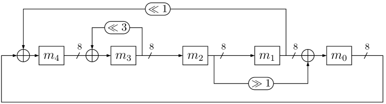
(b) Representation

Figure 17: An LFSR with efficient software design.

Let us now also compare a word oriented LFSR picked using our algorithm to the SNOW2.0 LFSR defined in [7]. The two LFSRs are respectively described in Appendix -B and in Appendix -C.

These two LFSRs output $m$-sequences of degree 512. We compare the diffusion delay and the throughput in software for those two LFSRs:

• The diffusion delay of the SNOW LFSR is 49 compared to 33 for our LFSR.

• The cost of one clock is 8 cycles for the SNOW LFSR using the sliding window implementation as proposed in [7] (this technique could be only applied for a Fibonacci LFSR). The cost for this LFSR implemented using classical implementation is 20 cycles. The cost for our LFSR is 33 cycles.

As presented the diffusion delay is better for our LFSR. However, the cost of one clock is higher in our case. This is due to the fact that the SNOW LFSR is sparse (three feedbacks) while ours has 8 feedbacks. Moreover, the computations are made using precomputed tables which leads to a better cost. However, the hardware implementation of our own LFSR has a really low cost (it fulfills the hardware design criteria we require in the previous section: critical path of length 1, fan-out of 2) whereas the SNOW2.0 LFSR could not be efficiently implemented in hardware due to the precomputed tables.

V-D Conclusion

To sum up the results given in this section, we have proposed two algorithms one for hardware purpose, one for software purpose that allow to build efficient LFSRs with a low diffusion delay and good implementation criteria. Moreover, building an LFSR using Alg. 16 leads to an LFSR with good cryptographic properties with an efficient implementation both in software and in hardware.

VI Conclusion

In this paper, we have shown how to link together matrix representations and polynomial representations for efficient LFSMs, LFSRs and windmill LFSRs constructions. Those new representations lead to efficient implementations both in software and in hardware. We have compared new Ring LFSR constructions with LFSRs used in several stream ciphers and we have shown that Ring LFSRs have always a better diffusion delay with better hardware performances and good software performances.

In further works, we aim at more precisely looking at the case of an LFSM with $\ell$ output bits to give equivalent and general representations. We also want to generalize those new results to Finite State Machines that are no more linear. The same kind of generalization could be efficiently applied to Feedback with Carry Shift Registers (FCSRs) or to Algebraic Feedback Shift Registers (AFSRs).

-A Example of a Ring LFSR of size 128 bits

We describe a Ring LFSR of size 128 bits. The transition matrix $A=(a_{i,j})$ is given by:

$$\left\{\begin{array}[]{l}a_{i,i+1}=1\text{ for all }0\leq i<127\\ a_{127,0}=1\\ a_{i,j}=1\text{ for }(i,j)\in{\mathcal{F}}\end{array}\right.$$

where ${\mathcal{F}}$ is the set:

$$\left\{\begin{array}[]{cccccccc}(4,78),&(5,19),&(8,44),&(9,106),\\ (10,70),&(12,14),&(14,115),&(15,55),\\ (17,82),&(21,64),&(22,12),&(25,127),\\ (27,107),&(28,112),&(31,59),&(34,111),\\ (35,48),&(37,36),&(38,23),&(39,88),\\ (43,37),&(44,26),&(46,60),&(47,100),\\ (49,24),&(50,25),&(51,2),&(51,27),\\ (55,124),&(57,113),&(59,71),&(61,29),\\ (69,123),&(72,52),&(73,118),&(77,46),\\ (80,74),&(81,83),&(83,98),&(87,53),\\ (88,73),&(91,47),&(93,10),&(94,21),\\ (95,93),&(97,13),&(98,117),&(99,50),\\ (100,3),&(101,104),&(104,1),&(105,114),\\ (106,108),&(107,105),&(109,4),&(111,28),\\ (112,68),&(113,42),&(114,31),&(119,18),\\ (120,49),&(121,32),&(123,94),&(124,6)\end{array}\right\}$$

This LFSR has a primitive connection polynomial. It has a cost of 64 adders, a fan-out equal to 2 and a critical path of 1, and a diffusion delay of 27.

-B Description of the LFSR in SNOW 2.0 over ${\mathbb{F}}_{2}$

We give here a description of the LFSR used in SNOW 2.0 [7] seen as a LFSR over ${\mathbb{F}}_{2}$.

First this LFSR is defined as a Fibonacci LFSR over ${\mathbb{F}}_{2^{32}}$. The field ${\mathbb{F}}_{2^{32}}$ is defined as an extension of ${\mathbb{F}}_{2^{8}}$ to allow an efficient implementation and to prevent the guess-and-determine attack presented in [42].

The implementation is based upon the multiplication by $\alpha\in{\mathbb{F}}_{2^{32}}$ satisfying $\alpha\cdot(c_{3}\alpha^{3}+c_{2}\alpha^{2}+c_{1}\alpha^{1}+c_{0})=(c_{2}\alpha^{3}+c_{1}\alpha^{2}+c_{0}\alpha)+c_{3}\cdot V$ with $V$ an element in ${\mathbb{F}}_{2^{32}}$. We denote $M_{\alpha}$ the matrix of this linear application seen over ${\mathbb{F}}_{2}^{32}$:

$$M_{\alpha}=\left(\begin{array}[]{ccc|c|c|c|c}0&0&0&&&&\\ I_{8}&&(0)&V_{0}&V_{1}&\dots&V_{7}\\ &I_{8}&&&&&\\ (0)&&I_{8}&&&&\\ \end{array}\right)$$

where

$$\left\{\begin{array}[]{c}V_{0}={}^{t}(\texttt{0xE19FCF13})\\ V_{1}={}^{t}(\texttt{0x6B973726})\\ V_{2}={}^{t}(\texttt{0xD6876E4C})\\ V_{3}={}^{t}(\texttt{0x05A7DC98})\\ V_{4}={}^{t}(\texttt{0x0AE71199})\\ V_{5}={}^{t}(\texttt{0x1467229B})\\ V_{6}={}^{t}(\texttt{0x28CE449F})\\ V_{7}={}^{t}(\texttt{0x50358897})\end{array}\right.$$

Then the transition matrix of the LFSR of SNOW2.0 is presented in Figure 18.

$$\left(\begin{array}[]{cccccccccccccccc}&I_{32}&&&&&&&&&&&&&&\\ &&I_{32}&&&&&&&&&&&&&\\ &&&I_{32}&&&&&&&&&&&&\\ &&&&I_{32}&&&&&&&(0)&&&&\\ &&&&&I_{32}&&&&&&&&&&\\ &&&&&&I_{32}&&&&&&&&&\\ &&&&&&&I_{32}&&&&&&&&\\ &&&&&&&&I_{32}&&&&&&&\\ &&&&&&&&&I_{32}&&&&&&\\ &&&&(0)&&&&&&I_{32}&&&&&\\ &&&&&&&&&&&I_{32}&&&&\\ &&&&&&&&&&&&I_{32}&&&\\ &&&&&&&&&&&&&I_{32}&&\\ &&&&&&&&&&&&&&I_{32}&\\ &&&&&&&&&&&&&&&I_{32}\\ M_{\alpha}&0&I_{32}&0&0&0&0&0&0&0&0&(M_{\alpha})^{-1}&0&0&0&0\\ \end{array}\right)$$

Figure 18: Transition matrix of SNOW2.0

-C Example of a word-oriented LFSR of size 512 bits

We give in Figure 19 a description of a word-oriented LFSR of length 512 with words of 32 bits. The grid in the matrix is drawn for readability.

$$\left(\begin{array}[]{ccc|ccc|ccc|ccc|ccc|c}&I_{32}&&&&&&&&&&&&&&\\ &&I_{32}&&&&&&R^{14}&&&&&&&\\ &&&I_{32}&&&L^{8}&&&&&&&&&\\ \hline\cr&&&&I_{32}&&&&&&(0)&L^{12}&&&&\\ &&&&&I_{32}&&&&&&&&&&\\ &&&&&L^{2}&I_{32}&&&&&&&&&\\ \hline\cr&&&&&&&I_{32}&&&&&&&&\\ &&&&&&&&I_{32}&&&&&&R^{11}&\\ L^{13}&&&&&&&&&I_{32}&&&&&&\\ \hline\cr&&&&(0)&&&&&&I_{32}&&&&&\\ &&&&&&&&&&&I_{32}&&&&\\ &&&&&&&&&&&&I_{32}&&&\\ \hline\cr&&&&&&&&&&&&&I_{32}&&\\ &&&&&&&&&&&R^{13}&&&I_{32}&\\ &&&&&&&&&&&&&&&I_{32}\\ \hline\cr I_{32}&&R^{10}&&&&&&&&&&&&&\\ \end{array}\right)$$

Figure 19: Transition matrix of a word oriented LFSR

References

- [1] S. W. Golomb, Shift Register Sequences. Aegen Park Press, 1981.
- [2] Y. Roggeman, “Varying feedback shift registers,” in EUROCRYPT, ser. Lecture Notes in Computer Science, vol. 434. Springer-Verlag, 1989, pp. 670–679.
- [3] D. Kagaris, “A similarity transform for linear finite state machines,” Discrete Applied Mathematics, vol. 154, no. 11, pp. 1570–1577, 2006.
- [4] B. J. M. Smeets and W. G. Chambers, “Windmill generators: A generalization and an observation of how many there are,” in EUROCRYPT, 1988, pp. 325–330.
- [5] Bluetooth, “Specification of the bluetooth system, volume 1: Core, v1.1,” Bluetooth SIG, February 2001.
- [6] C. Lauradoux, “Extended Windmill Polynomials,” in IEEE International Symposium on Information Theory - ISIT 2009. Seoul, Korea: IEEE, june-july 2009, pp. 1120–1124.
- [7] P. Ekdahl and T. Johansson, “A new version of the stream cipher SNOW,” in Selected Areas in Cryptography – SAC 2002, ser. Lecture Notes in Computer Science, vol. 2295. Springer-Verlag, 2002, pp. 47–61.
- [8] NESSIE, “Nessie phase 1 : selection of primitives,” https://www.cryptonessie.org/, 2001.
- [9] H. Stone, “Discrete Mathematical Structures and their Applications. Sci. Res,” Associates, Chicago, 1973.
- [10] M. Goresky and A. Klapper, “Algebraic shift register sequences,” 2009, avalaible at http://cs.engr.uky.edu/~klapper/algebraic.html.
- [11] K. Cattell and J. C. Muzio, “An Explicit Similarity Transform between Cellular Automata and LFSR Matrices,” Finite Fields and Their Applications, vol. 4, no. 3, pp. 239 – 251, 1998.
- [12] I. Goldberg and D. Wagner, “Architectural considerations for cryptanalytic hardware,” CS252 Report¡ http://www. cs. berkeley. edu/~ iang/isaac/hardware, 1996.
- [13] P. Leglise, F. Standaert, G. Rouvroy, and J.-J. Quisquater, “Efficient implementation of recent stream ciphers on reconfigurable hardware devices,” in 26th Symposium on Information Theory in the Benelux, 2005, pp. 261–268.
- [14] A. Joux and P. Delaunay, “Galois lfsr, embedded devices and side channel weaknesses,” in INDOCRYPT, ser. Lecture Notes in Computer Science, R. Barua and T. Lange, Eds., vol. 4329. Springer, 2006, pp. 436–451.
- [15] K. Cattell and J. C. Muzio, “Analysis of One-Dimensional Linear Hybrid Cellular Automata over GF(q),” IEEE Trans. Comput., vol. 45, no. 7, pp. 782–792, 1996.
- [16] ——, “Synthesis of One-Dimensional Linear Hybrid Cellular Automata,” IEEE Trans. Computer-Aided Design, vol. 15, pp. 325–335, 1996.
- [17] G. Mrugalski, J. Rajski, and J. Tyszer, “Ring generators - new devices for embedded test applications,” IEEE Trans. on CAD of Integrated Circuits and Systems, vol. 23, no. 9, pp. 1306–1320, 2004.
- [18] C. Dufaza, “Theoretical properties of lfsrs for built-in self test,” Integration, vol. 25, no. 1, pp. 17–35, 1998.
- [19] J. Daemen and V. Rijmen, The Design of Rijndael: AES - The Advanced Encryption Standard. Springer, 2002.
- [20] C. Berbain, O. Billet, A. Canteaut, N. Courtois, H. Gilbert, L. Goubin, A. Gouget, L. Granboulan, C. Lauradoux, M. Minier, T. Pornin, and H. Sibert, “Sosemanuk, a fast software-oriented stream cipher,” in The eSTREAM Finalists, ser. Lecture Notes in Computer Science, M. J. B. Robshaw and O. Billet, Eds. Springer, 2008, vol. 4986, pp. 98–118.
- [21] M. Hell, T. Johansson, A. Maximov, and W. Meier, “The grain family of stream ciphers,” in The eSTREAM Finalists, ser. Lecture Notes in Computer Science, M. J. B. Robshaw and O. Billet, Eds. Springer, 2008, vol. 4986, pp. 179–190.
- [22] E. S. C. P. eSTREAM, “The current estream portfolio,” eSTREAM, ECRYPT Stream Cipher Project, 2008, http://www.ecrypt.eu.org/stream.
- [23] E. Filiol and C. Fontaine, “A new ultrafast stream cipher design: Cos ciphers,” in Cryptography and Coding, 8th IMA International Conference, Cirencester, UK, December 17-19, 2001, Proceedings, ser. Lecture Notes in Computer Science, B. Honary, Ed., vol. 2260. Springer, 2001, pp. 85–98.
- [24] J.-P. Aumasson, L. Henzen, W. Meier, and M. Naya-Plasencia, “Quark: A lightweight hash,” in Cryptographic Hardware and Embedded Systems, CHES 2010, 12th International Workshop, Santa Barbara, CA, USA, August 17-20, 2010. Proceedings, ser. Lecture Notes in Computer Science, S. Mangard and F.-X. Standaert, Eds., vol. 6225. Springer, 2010, pp. 1–15.
- [25] C. Shannon, “Communication theory of secrecy systems,” Bell System Technical Journal, Vol 28, pp. 656-715, October 1949.
- [26] F. Panneton and P. L’Ecuyer, “On the xorshift random number generators,” ACM Trans. Model. Comput. Simul., vol. 15, no. 4, pp. 346–361, 2005.
- [27] H. Feistel, “Cryptography and computer privacy,” j-SCI-AMER, vol. 228, no. 5, pp. 15–23, May 1973.
- [28] A. F. Webster and S. E. Tavares, “On the design of s-boxes,” in CRYPTO, 1985, pp. 523–534.
- [29] S. W. Golomb and G. Gong, Signal Design for Good Correlation: For Wireless Communication, Cryptography, and Radar. New York, NY, USA: Cambridge University Press, 2004.
- [30] P. Flajolet and A. M. Odlyzko, “Random mapping statistics,” in EUROCRYPT, 1989, pp. 329–354.
- [31] P. L’Ecuyer, “Maximally equidistributed combined Tausworthe generators,” Math. Comput., vol. 65, no. 213, pp. 203–213, 1996.
- [32] F. Arnault, T. P. Berger, C. Lauradoux, M. Minier, and B. Pousse, “A new approach for fcsrs,” in Selected Areas in Cryptography, 2009, pp. 433–448.
- [33] M. Hell and T. Johansson, “Breaking the f-fcsr-h stream cipher in real time,” in ASIACRYPT, 2008, pp. 557–569.
- [34] L.-T. Wang and E. J. McCluskey, “Hybrid designs generating maximum-length sequences,” IEEE Trans. on CAD of Integrated Circuits and Systems, vol. 7, no. 1, pp. 91–99, 1988.
- [35] T. G. Lewis and W. H. Payne, “Generalized feedback shift register pseudorandom number algorithm,” J. ACM, vol. 20, no. 3, pp. 456–468, 1973.
- [36] M. Matsumoto and Y. Kurita, “Twisted GFSR generators,” ACM Trans. Model. Comput. Simul., vol. 2, no. 3, pp. 179–194, 1992.
- [37] M. Matsumoto and T. Nishimura, “Mersenne twister: A 623-dimensionally equidistributed uniform pseudo-random number generator,” ACM Trans. Model. Comput. Simul., vol. 8, no. 1, pp. 3–30, 1998.
- [38] H. Niederreiter, “The multiple-recursive matrix method for pseudorandom number generation,” Finite Fields Appl., vol. 1, no. 1, pp. 3–30, 1995.
- [39] G. Marsaglia, “Xorshift RNGs,” Journal of Statistical Software, vol. 8, no. 14, pp. 1–6, 2003. [Online]. Available: http://www.jstatsoft.org/v08/i14;http://www.jstatsoft.org/v08/i14/xorshift.pdf
- [40] B. Tsaban and U. Vishne, “Efficient linear feedback shift registers with maximal period,” Finite Fields and Their Applications, vol. 8, p. 256 267, 2002.
- [41] B. Preneel, “Fse’94 - introduction,” in FSE, 1994, pp. 1–5.
- [42] P. Hawkes and G. G. Rose, “Guess-and-determine attacks on snow,” in Selected Areas in Cryptography, ser. Lecture Notes in Computer Science, K. Nyberg and H. M. Heys, Eds., vol. 2595. Springer, 2002, pp. 37–46.
- [43] M. J. B. Robshaw and O. Billet, Eds., New Stream Cipher Designs - The eSTREAM Finalists, ser. Lecture Notes in Computer Science. Springer, 2008, vol. 4986.