A new proof of the Herman-Avila-Bochi formula for Lyapunov exponents of -cocycles
Alexandre T. Baraviera
Departamento de Matemática
Universidade Federal do Rio Grande do Sul
Porto Alegre, RS, Brasil
baravi@mat.ufrgs.br, João Lopes Dias
Departamento de Matemática and Cemapre, ISEG
Universidade Técnica de Lisboa
Rua do Quelhas 6, 1200-781 Lisboa, Portugal
jldias@iseg.utl.pt and Pedro Duarte
Departamento de Matemática and Cmaf
Faculdade de Ciências
Universidade de Lisboa
Campo Grande, Edifício C6, Piso 2
1749-016 Lisboa, Portugal
pduarte@ptmat.fc.ul.pt
Abstract.
We study the geometry of the action of on the projective line in order to present a new and simpler proof of the Herman-Avila-Bochi formula.
This formula gives the average Lyapunov exponent of a class of 1-families of -cocycles.
1. Introduction
A fundamental problem in smooth dynamics is the determination of the Lyapunov exponents of a given system.
These values correspond to the exponential rate of divergence or convergence of nearby orbits along prescribed directions.
A positive Lyapunov exponent implies hyperbolic behaviour of orbits, which might produce very complicated dynamics.
On the other hand, a negative Lyapunov exponent indicates that the orbits are fast converging and thus dynamics should be simpler.
Lyapunov exponents exist almost everywhere in phase space by the Oseledets theorem. However, their computation is typically a hard problem that has only been overcome by the use of numerical techniques.
In fact, there are very few non-trivial examples outside uniform hyperbolicity for which their values (or even the signs) have been computed analytically.
Criteria for positive Lyapunov exponents for non-uniformly hyperbolic systems can be found in [6, 7, 8].
In this paper we treat a remarkable example where the average Lyapunov exponents of families of cocycles can be explicitly computed.
Herman [5] was the first to present it in the context of products of -matrices over an ergodic transformation, and found a lower bound for the average upper Lyapunov exponent.
Later, Avila and Bochi [2] showed that Herman’s lower bound was the actual value of the average exponent.
We present below the setting and results related to this problem, and give an alternative proof of the Herman-Avila-Bochi formula.
Our approach simplifies considerably the analysis by looking at simple geometric consequences of the action of the matrices on the projective line .
Let be a probability space, a measurable -preserving ergodic transformation , and a -integrable function .
We want to study the dynamics of the linear cocycle
given by
Its iterations are also linear cocycles
where
Due to the above vector bundle structure we call the space the base, whilst is the fiber.
We deal with the question of obtaining the largest Lyapunov exponent on the fiber for the above cocyles.
This is given by the asymptotic exponential growth of the norm of the product of matrices, measured by the fiber upper Lyapunov exponent of ,
(1.1)
By considering the rotation by an angle ,
(1.2)
we focus on the 1-family of cocycles .
Using a sub-harmonicity “trick”, Herman showed the following inequality for the average Lyapunov exponent inside this family.
Roughly, Herman’s method consists in showing that the function
has a sub-harmonic extension to the
unit disk in the complex plane.
The inequality then follows from the sub-harmonicity property.
Later, under the same assumptions, Avila and Bochi improved Herman’s inequality by showing that actually equality occurs.
As an example, this theorem applies immediately to the cocycle over an ergodic rotation on the circle with
and .
We then have and so is constant in the family.
The Herman-Avila-Bochi formula above gives .
We remark that examples as this one are delicate since a -generic -cocycle is uniformly hyperbolic or it has zero Lyapunov exponent almost everywhere [3].
Notice that for ,
(see [2, Proposition 3]).
Using Birkhoff’s ergodic theorem,
Avila and Bochi reduce the proof of Theorem 2 to the following one (see [2, Theorem 12]), where stands for the logarithm of the spectral radius of .
To prove the above formula they show that the sub-harmonic extension of
as in Herman’s trick, is in fact harmonic.
We present here an alternative proof of Theorem 3 based on a simple change of variable argument, which exploits instead the geometry of the action of on the projective line .
In section 2 we present some properties of the -action on , and complete our proof of Theorem 3 in section 3.
2. Symmetries of Matrix Actions
Consider the circle group as a model of the real projective line and
denote by the normalized Haar measure on .
Given let denote the line spanned by the vector
For a matrix the action of on is characterized by the relation
(2.1)
Its derivative is related to expansivity by
(2.2)
Moreover, define as
Notice that induces a well-defined map from
to , where the rotation matrices are defined in (1.2).
The function can thus be characterized by the eigenspace relation
(2.3)
Finally, take to be a function which measures the expansivity of the action of as
We then have the following properties.
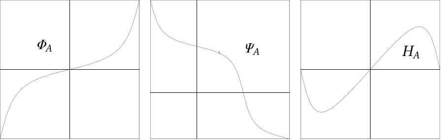
Proposition 1.
For every non-orthogonal matrix there is
a unique analytic map such that:
(1)
,
(2)
,
(3)
,
(4)
,
(5)
.
Figure 1. Functions , and
Proof. The uniqueness of such is obvious since the pre-image of each
regular value consists exactly of two points which must be inter-changed by .
By singular value decomposition, there exist and such that , where
Let with
We claim that is the required involution.
Since , we have and item 1 follows.
Notice also that
Hence,
which proves item 3.
Next assume that is symmetric. We have , i.e. ,
and for this case
is an isometric involution.
Thus,
The general case, where , now follows because is a constant function.
This implies that and share the same involution
.
As remarked above .
Therefore,
Finally, item 5 follows from item 4 since .
In our proof of the Herman-Avila-Bochi formula we will use the following abstract change of variables argument.
Proposition 2.
Consider an integrable function and a smooth involution
such that .
Then,
Proof. Let and , so that
and . So,
Similarly, .
Hence, the claim follows.
Our next proposition is a special case of Theorem 3.
The proof illustrates how the previous argument applies.
Proposition 3.
For any matrix ,
Proof. We will use the change of variable .
Notice first that is elliptic iff lies outside the range of , in which case the logarithm of the spectral radius of is zero, i.e. .
For the remaining values of , the eigenspace property (2.3) implies that .
Therefore,
On the first step, the factor appears because the map covers twice the set of parameters
which correspond to a real eigenvalue of .
The second equality follows because
and have the same sign for every .
Then we use item 5 of Proposition 1,
and the final step is a consequence of Proposition 2.
3. Matrix Sequence Actions
We call matrix word to any finite sequence of matrices
with , and is the length of the word.
So, we denote by the space of all -matrix words of length .
For such a word we define the product
Given any other matrix word , we have
where stands for the concatenated word
.
Moreover, we choose the maps
and
by
respectively.
Proposition 4.
Given any word ,
there exists analytic functions , , implicitely
defined by
.
Proof. The map
is an expanding map of degree .
So, for each
there are exactly points , such that
. By an implicit function theorem argument,
locally, each is an analytic function of ,
and we are left to prove that these local functions can be glued to form
global analytic functions.
By defining as the union of these local manifolds, it is enough to prove that is a compact -dimensional
manifold with connected components.
We can write as a pre-image
of the map
defined by .
Its derivative is
so has no critical points and is a compact analytic -dimensional manifold.
Since is a map of zero degree,
induces a linear endomorphism on the homology space
whose action is given by the matrix
Thus, must be the union of
homotopically non-trivial closed curves, which are precisely the graphs of
the functions .
The functions can also be characterized by the eigenspace relation
(3.1)
which implies that
That is, the matrix has the real eigenvector iff
for some .
This shows the following proposition.
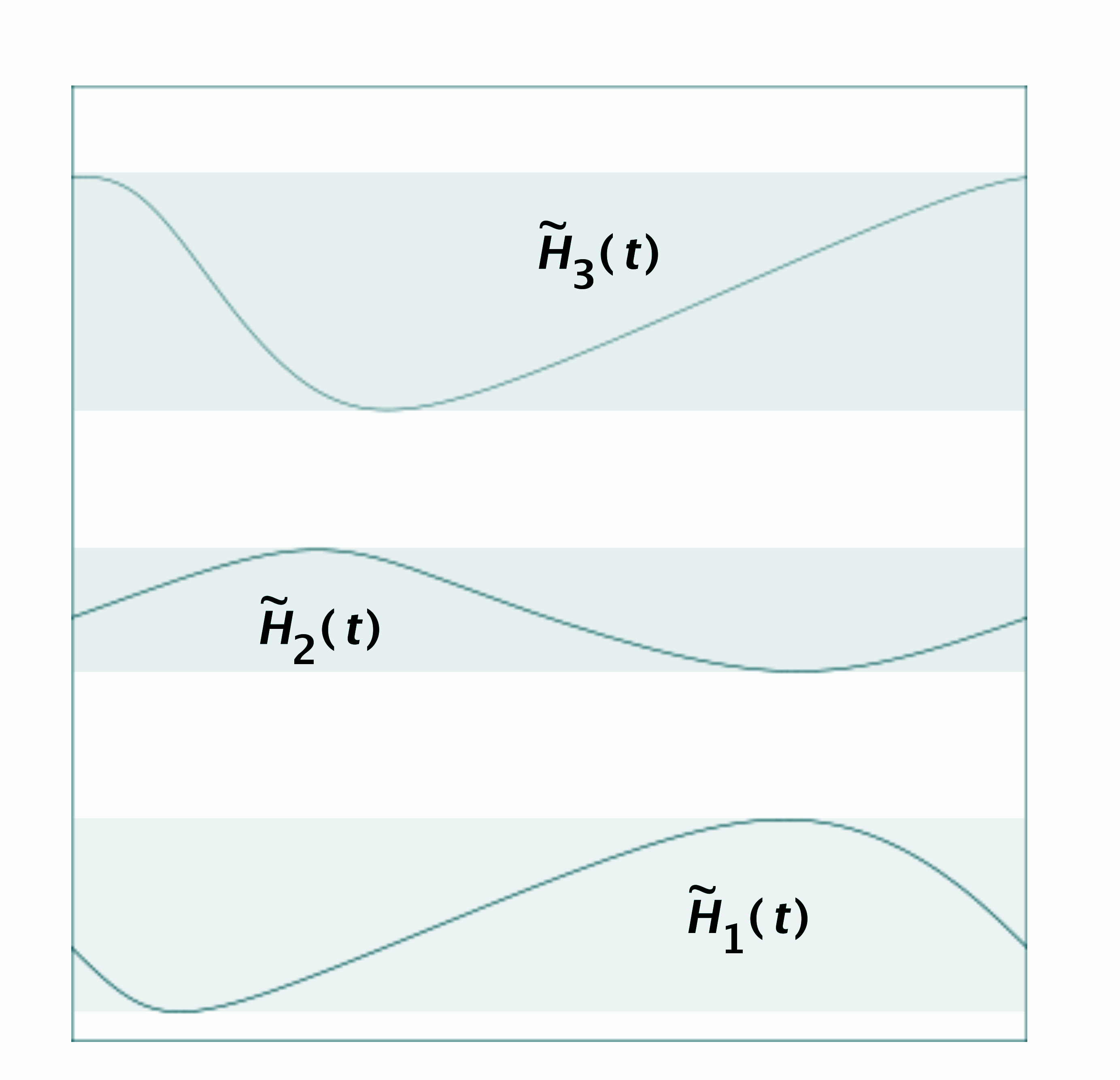
Proposition 5.
The matrix is elliptic iff is not in the range of any of the functions
with .
Moreover,
whenever for some
and . Otherwise, .
Figure 2. Hyperbolic regions
Given we define
so that .
We also define
Proposition 6.
Proof. Let denote the range of .
Performing the change of variables in each interval
, by Proposition 5 we have
The factor appears on the third step because the map
is a double cover of the interval .
The next step uses again Proposition 5.
Differentiating the relation
, which implicitely defines
, we obtain
with .
Hence, since , the numbers
,
have the same sign, which explains the fifth step. Step six follows by cocycle additivity,
and by exchanging the two summations, we complete the proof.
Lemma 1.
Given a matrix word and , the map
is an expanding map on with degree which preserves the Haar measure on .
Proof. Denote by the Haar measure, both on , and on
.
Let be the unit disk.
For each matrix
define by
. Then , where
is the map .
Consider the Möbius transformation
, which maps onto and
let .
The fundamental formula of trigonometry implies
that .
Notice that is a continuous group isomorphism. Hence .
Define now ,
which extends to a Möbius transformation on the Riemann sphere that preserves the circle .
The linear fractional map satisfies the symmetry relation
It has a single zero inside the disk , and a single pole outside.
With this notation, define
So, . Now, is a rational function satisfying the symmetry relation
with zeros inside the disk , and poles outside111
Functions with these properties are finite Blaschke products, see [4]..
The map is analytic on with . We claim that
this property implies that ,
which in turn will imply , and finish the proof.
To see this, take any continuous function . By the Dirichelet principle
this function has a continuous extension
which is harmonic on . We refer it as the harmonic extension of .
Since is analytic on ,
is the harmonic extension of . Therefore, by the Poisson formula
which implies that .
Proposition 7.
For and ,
Proof. We have for the matrix word ,
and hence
(3.2)
Differentiating (3.2) w.r.t. and we get respectively
Hence
(3.3)
Write . Differentiating the defining relation
and writing
for we obtain by (3.3) that
By Lemma 1,
since the points are the pre-images of by the measure preserving expanding map
,
Similarly,
because the points are the pre-images of by the measure preserving expanding map
.
Proposition 8.
For each ,
Proof. By definition we have .
Setting
since the matrices
and are conjugate
by we get
and hence, for ,
Differentiating this relation we obtain
Proposition 9.
For each ,
Proof. By Proposition 8 it is enough to consider the case .
Then combining propositions 7 and 2, we get the third
and fourth equalities below
This work was partially supported by Fundação para a Ciência e a Tecnologia through the project “Randomness in Deterministic Dynamical Systems and Applications” ref. PTDC/MAT/105448/2008.
References
[1]
[2] A. Avila and J. Bochi, A formula with some applications to the theory of Lyapunov exponents, Israel Journal of Mathematics 131 (2002), 125–137.
[3]J. Bochi, Genericity of zero Lyapunov exponents, Ergodic Theory Dynam. Systems 22 (2002), 1667–1696.
[4] J. Conway, Functions of One Complex Variable II,
Graduate Texts in Mathematics 159, Springer-Verlag (1995).
[5] M. Herman, Une méthode pour minorer les exposants de Lyapounov et quelques exemples montrant le caractère local d’un théorème d’ Arnold et de Moser sur le tore de dimension , Commentarii Mathematici Helvetici 58 (1983), 453–502.
[6] A. Katok, Infinitesimal Lyapunov functions, invariant cone families and stochastic properties of smooth dynamical systems. With the collaboration of Keith Burns., Ergodic Theory Dynam. Systems 14 (1994), 757–785.
[7] R. Markarian, Non-uniformly hyperbolic billiards, Ann. Fac. Sci. Toulouse, VI. Sér., Math. 3 (1994), 223–257.
[8] M. Wojtkowski, Invariant families of cones and Lyapunov exponents, Ergodic Theory Dynam. Systems 5 (1985), 145–161.