The Luminosity Function of Galaxies as modelled by the Generalized Gamma Distribution

Abstract

Two new luminosity functions of galaxies can be built starting from three and four parameter generalized gamma distributions. In the astrophysical conversion, the number of parameters increases by one, due to the addition of the overall density of galaxies. A third new galaxy luminosity function is built starting from a three parameter generalized gamma distribution for the mass of galaxies once a simple nonlinear relationship between mass and luminosity is assumed; in this case the number of parameters is five because the overall density of galaxies and a parameter that regulates mass and luminosity are added. The three new galaxy luminosity functions were tested on the Sloan Digital Sky Survey (SDSS) in five different bands; the results always produce a ”better fit” than the Schechter function. The formalism that has been developed allows to analyze the Schechter function with a transformation of location. A test between theoretical and observed number of galaxies as a function of redshift was done on data extracted from a two-degree field galaxy redshift survey.

02.50.Cw Probability theory; 98.62.Ve Statistical and correlative studies of properties (luminosity and mass functions; mass-to-light ratio )

1 Introduction

The luminosity function of galaxies $\Phi(L)dL$ (LF) is the number of galaxies per unit volume, $Mpc^{3}$, whose luminosity is comprised between $L$ and $L+dl$, see Section 3.7 in [1] or Section 1.12 in [2]. The luminosity, $L$, has physical units of $Watt~{}Hz^{-1}$ and therefore the band being considered should always be specified. In our case, we selected the data of the Sloan Digital Sky Survey (SDSS) which has five bands $u^{*}$ ($\lambda=3550\AA{})$, $g^{*}$ ($\lambda=4770\AA{})$, $r^{*}$ ($\lambda=6230\AA{})$, $i^{*}$ ($\lambda=7620\AA{})$ and $z^{*}$ ($\lambda=9130\AA{})$ with $\lambda$ denoting the wavelength of the CCD camera, see [3].

The Schechter LF of galaxies, see [4], is the more widely used function

$$\Phi(L)dL=(\frac{\Phi^{*}}{L^{*}})(\frac{L}{L^{*}})^{\alpha}\exp\bigl{(}{-\frac{L}{L^{*}}}\bigr{)}dL\quad,$$ (1)

where $\alpha$ sets the slope for low values of $L$, $L^{*}$ is the characteristic luminosity and $\Phi^{*}$ is the normalization. In the formula above, $L^{*}$ characterizes the break of the LF. As an example, $L\geq 0.1L^{*}$ defines a giant galaxy , see the text after formula (1.18) in [5]. An astronomical form of equation (1) can be deduced by introducing the distribution in absolute magnitude

$$\Phi(M)dM= (0.4ln10)\Phi^{*}10^{0.4(\alpha+1)(M^{*}-M)}$$ (2)

$$\times\exp\bigl{(}{-10^{0.4(M^{*}-M)}}\bigr{)}dM\quad,$$

where $M^{*}$ is the characteristic magnitude as derived from the data.

This function has three parameters that can be found by fitting the data. Over the years, many modifications have been made to the Schechter LF in order to improve its fit: we report two of them. When the fit of the rich clusters LF is not satisfactory a two-component Schechter-like function is introduced, see [6]

$$L_{max}>L>L_{Dwarf}:\quad\Phi(L)dL=(\frac{\Phi^{*}}{L^{*}})(\frac{L}{L^{*}})^{\alpha}\exp\bigl{(}{-\frac{L}{L^{*}}}\bigr{)}dL\quad,$$

(3)

$$L_{Dwarf}>L>L_{min}:\quad\Phi(L)dL=(\frac{\Phi_{Dwarf}}{L^{*}})(\frac{L}{L_{Dwarf}})^{\alpha_{Dwarf}}dL\quad,$$

where

$$\Phi_{Dwarf}=\Phi^{*}(\frac{L_{Dwarf}}{L^{*}})^{\alpha}\exp\bigl{(}{-\frac{L_{Dwarf}}{L^{*}}}\bigr{)}\quad.$$

This two-component function defined between the maximum luminosity, $L_{max}$, and the minimum luminosity, $L_{min}$, has five parameters because two additional parameters have been added: $L_{Dwarf}$ which represents the magnitude where dwarfs first dominate over giants and ${\alpha_{Dwarf}}$ which regulates the faint slope parameter for the dwarf population.

Another LF introduced in order to fit the case of extremely low luminosity galaxies is the double Schechter function with five parameters, see [7]:

$$\Phi(L)dL=\frac{dL}{L_{\ast}}\exp(-L/L_{\ast})\left[\phi_{\ast,1}\left(\frac{L}{L_{\ast}}\right)^{\alpha_{1}}+\phi_{\ast,2}\left(\frac{L}{L_{\ast}}\right)^{\alpha_{2}}\right]\quad,$$ (4)

where the parameters $\Phi^{*}$ and $\alpha$ which characterize the Schechter function have been doubled in $\phi_{\ast,1}$ and $\phi_{\ast,2}$. The strong dependence of LF on different environments such as voids, superclusters and supercluster cores was analyzed by [8] with

$$F(L)\mathrm{d}L\propto(L/L^{*})^{\alpha}(1+(L/L^{*})^{\gamma})^{(\delta-\alpha)/\gamma}\mathrm{d}(L/L^{*}),$$ (5)

where $\alpha$ is the exponent at low luminosities $(L/L^{*})\ll 1$, $\delta$ is the exponent at high luminosities $(L/L^{*})\gg 1$, $\gamma$ is a parameter of transition between the two power laws, and $L^{*}$ is the characteristic luminosity. The previous LFs leave a series of questions unanswered or partially answered:

• What is the function of introducing a transformation of location in the LF?

• Is it possible to model the data with just a single LF?

• Is it possible to deduce a LF for galaxies starting from the mass distribution of galaxies?

• Is it possible to improve the Schechter function by introducing a transformation of location?

• Does the new LF match the observed behavior of the number of galaxies for a given solid angle and flux as a function of the redshift?

In Section 2, this paper explores how a generalized gamma distribution can model two galaxy LFs. The method which allows the LF to be deduced for galaxies starting from a mass distribution as given by a generalized gamma is presented in Section 3. Section 4 reports the analytical and numerical results on the Schechter function with transformation of location. In Section 5, the redshift dependence of the Schechter function and one of the four new LFs are compared with data from the two-degree Field Galaxy Redshift Survey in the 2dFGRS catalogue.

2 The generalized gamma distribution

The generalized gamma distribution can be represented with three parameters, see [9, 10] or four parameters, see [11]. We will explore both cases in the following. In order to make a comparison between our LF and the Schechter LF, we first down-loaded the data of the LF of galaxies in the five bands of SDSS adopted in [12]; they are available at: http://cosmo.nyu.edu/blanton/lf.html. In the previous paper, [12], the basic assumption was to consider a Friedmann-Robertson-Walker cosmological world model with matter density $\Omega_{0}=0.3$, vacuum pressure $\Omega_{\Lambda}=0.7$ and Hubble constant $H_{0}=100$ $h$ km s^-1 Mpc^-1 with $h=1$. The data contain the absolute magnitude, the value of the LF for that magnitude and the error of the LF.

The LF of galaxies as obtained from astronomical observations ranges in magnitude from a minimum value, $M_{min}$, to a maximum value, $M_{max}$; details can be found in [13] and [14]. A nonlinear fit through the Levenberg–Marquardt method (subroutine MRQMIN in [15]) allows the determination of the parameters, but the first derivative of the LF with respect to the unknown parameters should be provided. The merit function $\chi^{2}$ can be computed as

$$\chi^{2}=\sum_{j=1}^{n}(\frac{LF_{theo}-LF_{astr}}{\sigma_{LF_{astr}}})^{2}\quad,$$ (6)

where $n$ is number of data and the two indices $theo$ and $astr$ stand for theoretical and astronomical, respectively.

Particular attention should be paid to the number of unknown parameters in the LF: three for the Schechter function (formula (2)), four for formula  (21), four for the Schechter function with transformation of location (formula (30)), five as represented by formula (28) and five for formula (16). A reduced merit function $\chi_{red}^{2}$ can be computed as

$$\chi_{red}^{2}=\chi^{2}/NF\quad,$$ (7)

where $NF=n-k$, $n$ is the number of data and $k$ is the number of parameters. The Akaike information criterion ($AIC$), see [16] , is defined as

$$AIC=2k-2ln(L)\quad,$$ (8)

where $L$ is the likelihood function and $k$ the number of free parameters in the model. We assume a Gaussian distribution for the errors and the likelihood function can be derived from the $\chi^{2}$ statistic $L\propto\exp(-\frac{\chi^{2}}{2})$ where $\chi^{2}$ has been computed by equation (6), see [17], [18]. Now $AIC$ becomes

$$AIC=2k+\chi^{2}\quad.$$ (9)

The Bayesian information criterion ($BIC$), see [19], is

$$BIC=k~{}ln(n)-2ln(L)\quad,$$ (10)

where $L$ is the likelihood function, $k$ the number of free parameters in the model and $n$ the number of observations. The phrase ”better fit” used in the following means that the three statistical indicators : $\chi^{2}$, $AIC$ and $BIC$ are smaller for the considered LF than for the Schechter function .

2.1 The generalized gamma distribution with five parameters

The starting point is the probability density function (in the following PDF) named generalized gamma that we report exactly as in [11]:

$$G(x;a,b,c,k)=\frac{{\it k}\,\left({\frac{x-a}{b}}\right)^{c{\it k}-1}{{\rm e}^{-\left({\frac{x-a}{b}}\right)^{{\it k}}}}}{b\Gamma\left(c\right)}\quad,$$ (11)

where $\Gamma$ is the gamma function, $a$ is the location parameter, $b$ is the scale parameter, $c$ and $k$ are two shape parameters. The number of parameters is four and the astrophysical version of the previous PDF can be obtained by inserting $a=L_{a}$ , $x=L$ and $b=L^{*}$:

$$\Psi(L;L^{*},c,k,\Psi^{*})=\Psi^{*}\frac{{\it k}\,\left({\frac{L-L_{a}}{L^{*}}}\right)^{c{\it k}-1}{{\rm e}^{-\left({\frac{L-L_{a}}{L^{*}}}\right)^{{\it k}}}}}{L^{*}\Gamma\left(c\right)}\quad,$$ (12)

where $\Psi^{*}$ is a normalization factor which defines the overall density of galaxies, expressed as a number per cubic $Mpc$. The mathematical range of existence is $L_{a}\leq L<\infty$ and the number of parameters is five because $\Psi^{*}$ has been added. The averaged luminosity, ${\langle L\rangle}$, is:

$${\langle L\rangle}=\frac{{\it L^{*}}\,\Gamma\left({\frac{1+ck}{k}}\right)+{\it L_{a}}\,\Gamma\left(c\right)}{\Gamma\left(c\right)}\quad,$$ (13)

and the mode is at

$$L=\left({\frac{ck-1}{k}}\right)^{\frac{1}{k}}{\it L^{*}}+{\it L_{a}}\quad.$$ (14)

The relationships connecting the absolute magnitude $M$, $M^{*}$ and $M_{a}$ of a galaxy to its luminosity are:

$$\frac{L}{L_{\ast{\odot}}}=10^{0.4(M_{\ast{\odot}}-M)}\quad,~{}\frac{L^{*}}{L_{\ast{\odot}}}=10^{0.4(M_{\ast{\odot}}-M^{*})}\quad,~{}\frac{L_{a}}{L_{\ast{\odot}}}=10^{0.4(M_{\ast{\odot}}-M_{a})}\quad,$$ (15)

where $M_{\ast{\odot}}$ is the absolute magnitude of the sun in the considered band. As an example, the SDSS bands have $M_{\ast{\odot}}$= 4.48 in $z^{*}$ and $M_{\ast{\odot}}$= 6.32 in $u^{*}$, see [20]. A more convenient form of the LF in terms of the absolute magnitude $M$ is:

$$\Psi(M)dM={\it\Psi^{*}}\frac{0.4\,k\,\ln\left(10\right)\left({10}^{0.4\,{\it M^{*}}-0.4\,M}-{10}^{0.4\,{\it M^{*}}-0.4\,{\it M_{a}}}\right)^{ck-1}}{\Gamma\left(c\right)}\times$$

$${{\rm e}^{-\left({10}^{0.4\,{\it M^{*}}-0.4\,M}-{10}^{0.4\,{\it M^{*}}-0.4\,{\it M_{a}}}\right)^{k}}}{10}^{0.4\,{\it M^{*}}-0.4\,M}\,dM\quad.$$ (16)

The mode when expressed in magnitude is at

$$M=-1.085\,\ln\left(\left({\frac{ck-1}{k}}\right)^{\frac{1}{k}}{{\rm e}^{-0.921\,{\it M^{*}}}}+{{\rm e}^{-0.921\,{\it M_{a}}}}\right)\quad.$$ (17)

This data-oriented function contains the five parameters $c$, $k$, $M^{*}$, $M_{a}$ and $\Psi^{*}$ which can be derived from the operation of fitting observational data. The results are reported in Table 1 together with the number of elements $N$ belonging to the sample, $M_{min}$ and $M_{max}$ of the sample, the merit function $\chi^{2}$ and $\chi_{red}^{2}$, the $\chi^{2}$ and $\chi_{red}^{2}$ of the Schechter function as computed by us and the $\chi^{2}$ of the Schechter function as computed by [12].

Table 1: Parameters of fits to LF in SDSS Galaxies of five parameter function represented by formula (16).

$$\begin{array}[]{lccccc}\hline\cr parameter&u^{*}&g^{*}&r^{*}&i^{*}&z^{*}\\ \vskip 3.0pt plus 1.0pt minus 1.0pt\cr\hline\cr\vskip 3.0pt plus 1.0pt minus 1.0pt\cr M_{a}{}&-14.25&-15.55&-15.77&-16.52&-17.39\\ M^{*}-5\log_{10}h{}&-17.22&-18.29&-20&-20.01&-20.25\\ \Psi^{*}[h^{3}~{}Mpc^{-3}]&0.078&0.077&0.11&0.05&0.055\\ c&0.61&0.30&0.19&0.47&0.49\\ k&0.82&0.92&0.87&0.78&0.76\\ N&483&599&674&709&740\\ M_{min}&-20.65&-22.09&-22.94&-23.42&-23.73\\ M_{max}&-15.78&-16.32&-16.30&-17.21&-17.48\\ \chi^{2}&282&736&1766&1726&2136\\ \chi_{red}^{2}&0.59&1.24&2.64&2.45&2.90\\ AIC~{}k=5&292&746&1776&1736&2146\\ BIC~{}k=5&313&768&1799&1759&2169\\ \chi^{2}-Schechter&330&753&2260&2282&3245\\ \chi_{red}^{2}-Schechter&0.689&1.263&3.368&3.232&4.403\\ \chi^{2}-Blanton~{}2003&341&756&2276&2283&3262\\ AIC~{}k=3-Schechter&336&759&2266&2288&3253\\ BIC~{}k=3-Schechter&349&772&2279&2302&3265\\ \end{array}$$

The Schechter function, the new five parameter function represented by formula (16) and the data are reported in Figure 1, Figure 2, Figure 3, Figure 4, Figure 5, Figure 6, Figure 7, Figure 8, Figure 9, and Figure 10 where bands $u^{*}$, $g^{*}$, $r^{*}$, $i^{*}$ and $z^{*}$ are considered.

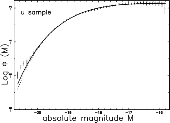
Figure 1: The luminosity function data of SDSS($u^{*}$) are represented with error bars. The continuous line fit represents our LF (16) and the dotted line represents the Schechter function.

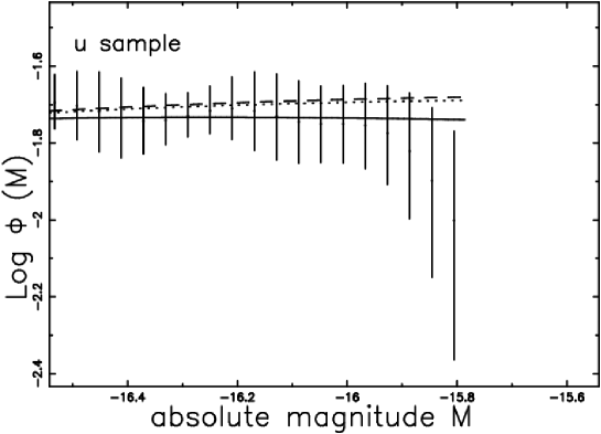
Figure 2: The luminosity function data of SDSS($u^{*}$) in the low luminosity region are represented by the error bar. The continuous line fit represents our LF (16), the dotted line represents the Schechter function as given by our data and the dashed line represents the Schechter function as given by [12].

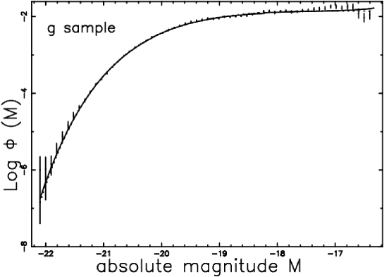
Figure 3: The luminosity function data of SDSS($g^{*}$) are represented with error bars. The continuous line fit represents our LF (16) and the dotted line represents the Schechter function.

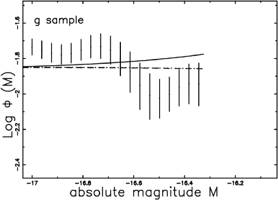
Figure 4: The luminosity function data of SDSS($g^{*}$) in the low luminosity region are represented by the error bar. The continuous line fit represents our LF (16), the dotted line represents the Schechter function as given by our data and the dashed line represents the Schechter function as given by [12].

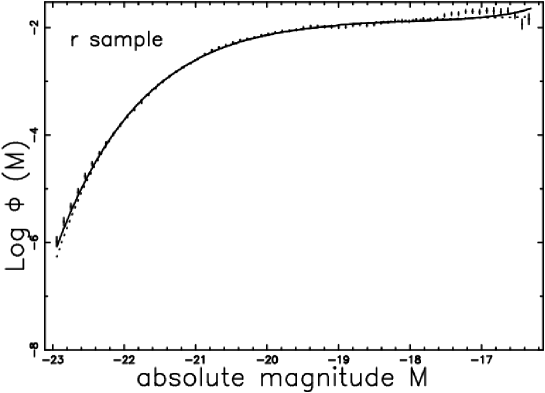
Figure 5: The luminosity function data of SDSS($r^{*}$) are represented with error bars. The continuous line fit represents our LF (16) and the dotted line represents the Schechter function.

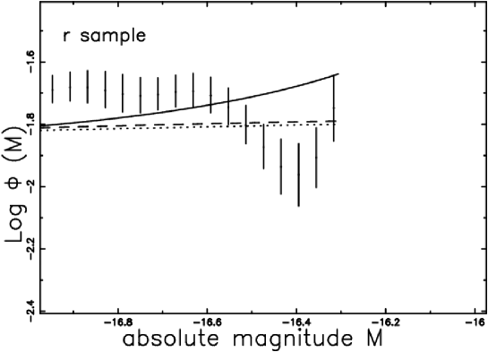
Figure 6: The luminosity function data of SDSS($r^{*}$) in the low luminosity region are represented with error bars. The continuous line fit represents our LF (16), the dotted line represents the Schechter function as given by our data and the dashed line represents the Schechter function as given by [12].

Figure 7: The luminosity function data of SDSS($i^{*}$) are represented with error bars. The continuous line fit represents our LF (16) and the dotted line represents the Schechter function.

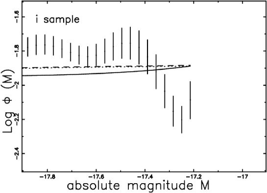
Figure 8: The luminosity function data of SDSS($i^{*}$) in the low luminosity region are represented with error bars. The continuous line fit represents our LF (16), the dotted line represents the Schechter function as given by our data and the dashed line represents the Schechter function as given by [12].

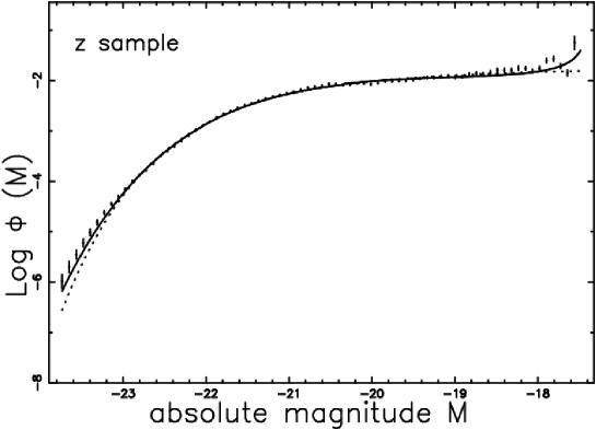
Figure 9: The luminosity function data of SDSS($z^{*}$) are represented with error bars. The continuous line fit represents our LF (16) and the dotted line represents the Schechter function.

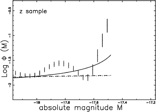
Figure 10: The luminosity function data of SDSS($z^{*}$) in the low luminosity region are represented with error bars. The continuous line fit represents our LF (16), the dotted line represents the Schechter function as given by our data and the dashed line represents the Schechter function as given by [12].

The flexiblity of the generalized gamma with five parameters to fit a sudden increase in the low luminosity region is clearly visible in Figure 10.

2.2 The generalized gamma distribution with four parameters

We can start from equation (11), inserting $a=0$, $x=L$ and $b=L^{*}$:

$$\Psi(L;L^{*},c,k,\Psi^{*})=\Psi^{*}\frac{{\it k}\,\left({\frac{L}{L^{*}}}\right)^{c{\it k}-1}{{\rm e}^{-\left({\frac{L}{L^{*}}}\right)^{{\it k}}}}}{L^{*}\Gamma\left(c\right)}\quad.$$ (18)

The mathematical range of existence is $0\leq L<\infty$ and the number of parameters is four because $a=0$ and $\Psi^{*}$ have been added. The averaged luminosity is

$${\langle L\rangle}=\frac{{\it L^{*}}\,\Gamma\left({\frac{1+ck}{k}}\right)}{\Gamma\left(c\right)}\quad,$$ (19)

and the mode is at

$$L=\left({\frac{ck-1}{k}}\right)^{\frac{1}{k}}{\it L^{*}}\quad.$$ (20)

The magnitude version of the LF is

$$\Psi(M)dM=\frac{{\Psi^{*}}\,0.4\,\ln\left(10\right)\,k{10}^{-0.4\,ck\left(M-\,{M^{*}}\right)}{{\rm e}^{-\,{10}^{-0.4\,\left(M-\,{M^{*}}\right)k}}}}{\Gamma\left(c\right)}dM\quad.$$ (21)

The mode when expressed in magnitude is at

$$M=-\frac{1.0857\,\ln\left({\frac{c{\it k}-1}{{\it k}}}\right)}{k}+{\it M^{*}}\quad.$$ (22)

This function contains the four parameters $c$, k$k$, $M^{*}$ and $\Psi^{*}$ and the numerical values obtained are reported in Table 2.

Table 2: Parameters for fits to LF in SDSS Galaxies with the four parameter function represented by formula (21).

$$\begin{array}[]{lccccc}\hline\cr parameter&u^{*}&g^{*}&r^{*}&i^{*}&z^{*}\\ \vskip 3.0pt plus 1.0pt minus 1.0pt\cr\hline\cr\vskip 3.0pt plus 1.0pt minus 1.0pt\cr M^{*}-5\log_{10}h&-17.34&-19.43&-20.25&-20.29&-20.76\\ \Psi^{*}[h^{3}~{}Mpc^{-3}]&0.101&0.231&0.65&0.097&0.2\\ c&0.47&0.08&0.02&0.247&0.10\\ k&0.842&1.019&0.93&0.839&0.864\\ \chi^{2}&283&747&2188&1866&2915\\ \chi_{red}^{2}&0.591&1.256&3.266&2.648&3.991\\ AIC~{}k=4&291&755&2196&1874&2921\\ BIC~{}k=4&307&773&2214&1893&2921\\ \chi^{2}Schechter&330&753&2260&2282&3245\\ \chi_{red}^{2}-Schechter&0.689&1.263&3.368&3.232&4.403\\ \chi^{2}Blanton~{}2003&341&756&2276&2283&3262\\ \end{array}$$

3 The generalized gamma distribution for mass

We assume that the masses of galaxies, $\mathcal{M}$, are distributed as a generalized gamma. We can start from equation (11) inserting $a=0$ , $x=\mathcal{M}$ and $b=\mathcal{M}^{*}$

$$\Psi(\mathcal{M};\mathcal{M}^{*},c,k,\Psi^{*})=\Psi^{*}\frac{{\it k}\,\left({\frac{\mathcal{M}}{\mathcal{M}^{*}}}\right)^{c{\it k}-1}{{\rm e}^{-\left({\frac{\mathcal{M}}{\mathcal{M}^{*}}}\right)^{{\it k}}}}}{\mathcal{M}^{*}\Gamma\left(c\right)}\quad.$$ (23)

This is a generalized gamma distribution with a scale parameter ${\mathcal{M}^{*}}$, c and k are shape parameters . The mathematical range of existence is $0\leq\mathcal{M}<\infty$ and the number of parameters is four because $\Psi^{*}$ has been added. The average value is

$${\langle{\mathcal{M}}\rangle}=\Psi^{*}{\mathcal{M}^{*}}\frac{\Gamma\left({\frac{1+ck}{k}}\right)}{\Gamma\left(c\right)}\quad.$$ (24)

We now follow the pattern fixed in [21] where the PDF representing the mass of galaxies was assumed to be a Kiang function, see [22]. The mass-luminosity relationship is assumed to follow a power law having the form

$$\frac{\mathcal{M}}{\mathcal{M}^{*}}=\left(\frac{L}{L^{*}}\right)^{\frac{1}{d}}\quad,$$ (25)

where $1/d$ is an exponent which connects the mass to luminosity. The PDF (23 ) is therefore transformed into the following form:

$$\Psi(L)dL=\Psi^{*}\frac{k\left({\frac{L}{{\it L^{*}}}}\right)^{\frac{ck-1}{d}}{\rm e}^{-\left({\frac{L}{L^{*}}}\right)^{\frac{k}{d}}}\left({\frac{L}{{\it L^{*}}}}\right)^{\frac{1}{d}}}{d\,\Gamma\left(c\right)L},$$ (26)

The mathematical range of existence is $0\leq L<\infty$ and the averaged luminosity, ${\langle L\rangle}$, is

$${\langle L\rangle}=\Psi^{*}\frac{{\it L^{*}}\,\Gamma\left({\frac{d+ck}{k}}\right)}{\Gamma\left(c\right)}\quad.$$ (27)

The magnitude version of the previous LF is:

$$\Psi(M)dM={\it\Psi^{*}}\frac{0.4\,{\it ak}\,{10}^{-0.4\,{\frac{c{\it ak}\,\left(-\,{\it M^{*}}+{\it M}\right)}{d}}}{{\rm e}^{-{10}^{-0.4\,{\frac{\left(-\,{\it M^{*}}+{\it M}\right){\it ak}}{d}}}}}\ln\left(10\right)}{\Gamma\left(c\right)d}\quad.$$ (28)

The mode expressed in magnitude is at

$$M=M^{*}-1.0857\,{\frac{\ln\left(c\right)d}{{\it k}}}\quad.$$ (29)

This function contains the five parameters $c$, $k$, $d$, $M^{*}$ and $\Psi^{*}$ and the numerical values obtained are reported in Table 3.

Table 3: Parameters of fits to LF in SDSS Galaxies of the five parameter function represented by formula (28) deduced from the mass-luminosity relationship.

$$\begin{array}[]{lccccc}\hline\cr parameter&u^{*}&g^{*}&r^{*}&i^{*}&z^{*}\\ \vskip 3.0pt plus 1.0pt minus 1.0pt\cr\hline\cr\vskip 3.0pt plus 1.0pt minus 1.0pt\cr M^{*}-5\log_{10}h&-17.34&-19.39&-20.18&-20.43&-20.53\\ \Psi^{*}[h^{3}~{}Mpc^{-3}]&0.101&0.19&0.33&0.12&0.11\\ c&0.47&0.1&0.05&0.17&0.22\\ k&0.855&1.029&0.93&0.88&0.824\\ d&1.015&1.024&1.023&1.018&1.017\\ \chi^{2}&283&751&2217&1896&3009\\ \chi_{red}^{2}&0.592&1.265&3.313&2.693&3.313\\ AIC~{}k=3&289&757&2223&1902&3015\\ BIC~{}k=3&314&783&2249&1929&3042\\ \chi^{2}~{}Schechter&330&753&2260&2282&3245\\ \chi_{red}^{2}-Schechter&0.689&1.263&3.368&3.232&4.403\\ \chi^{2}~{}Blanton~{}2003&341&756&2276&2283&3262\\ \end{array}$$

From a careful analysis of Table 3, it is possible to conclude that $1.015<d<1.024$. Because we have assumed that $L\propto\mathcal{M}^{d}$, the nonlinear relationship between mass and luminosity is a weak effect. A weak dependence of the parameter that regulates mass and luminosity has also been found in [23] when the PDF which represents the mass of galaxies is the product of two gamma variates with argument 2.

4 The Schechter function with transformation of location

The Schechter LF of galaxies once the location $L_{a}$ is introduced is:

$$\Phi(L)dL=(\frac{\Phi^{*}}{L^{*}})(\frac{(L-L_{a})}{L^{*}})^{\alpha}\exp\bigl{(}{-\frac{(L-L_{a})}{L^{*}}}\bigr{)}dL\quad,$$ (30)

and is characterized by four parameters.

The average luminosity, ${\langle L\rangle}$, is

$${\langle L\rangle}=\Phi^{*}(L^{*}\,\Gamma\left(2+\alpha\right)+L_{a}\,\Gamma\left(\alpha+1\right))\quad,$$ (31)

and the mode is at

$$L=\alpha\,L^{*}+L_{a}\quad,$$ (32)

or

$$M=-1.085\,\ln\left(\alpha\,{{\rm e}^{-0.921\,{\it M^{*}}}}+{{\rm e}^{-0.921\,{\it M_{a}}}}\right)\quad.$$ (33)

The magnitude version of this LF is

$$\Phi(M)dM=0.4\,\Phi^{*}\,\left({10}^{0.4\,M^{*}-0.4\,M}-\,{10}^{0.4\,M^{*}-0.4\,M_{a}}\right)^{\alpha}$$

$${{\rm e}^{-\,{10}^{0.4\,M^{*}-0.4\,M}+{10}^{0.4\,M^{*}-0.4\,M_{a}}}}{10}^{0.4\,M^{*}-0.4\,M}\ln\left(10\right)\quad.$$ (34)

This function contains the four parameters $\alpha$, $M_{a}$, $M^{*}$ and $\Phi^{*}$ and the numerical values obtained are reported in Table 4.

Table 4: Parameters of fits to LF in SDSS Galaxies of the four parameter Schechter function with location as represented by formula (34).

$$\begin{array}[]{lccccc}\hline\cr parameter&u^{*}&g^{*}&r^{*}&i^{*}&z^{*}\\ \vskip 3.0pt plus 1.0pt minus 1.0pt\cr\hline\cr\vskip 3.0pt plus 1.0pt minus 1.0pt\cr M^{*}-5\log_{10}h&-17.92&-19.37&-20.41&-20.83&-21.15\\ \Phi^{*}[h^{3}~{}Mpc^{-3}]&0.03&0.021&0.015&0.014&0.013\\ \alpha&-0.9&-0.84&-0.99&-1.02&-1.01\\ M_{a}~{}[mags]&-12.1&-14.87&-15.14&-12.72&-16.39\\ \chi^{2}&333&723&2108&2453&3133\\ \chi_{red}^{2}&0.69&1.21&3.14&3.47&4.25\\ AIC~{}k=4&341&731&2116&2451&3141\\ BIC~{}k=4&358&748&2134&2479&3159\\ \chi^{2}~{}Schechter&330&753&2260&2282&3245\\ \chi_{red}^{2}-Schechter&0.689&1.263&3.368&3.232&4.403\\ \chi^{2}~{}Blanton~{}2003&341&756&2276&2283&3262\\ \end{array}$$

From a careful analysis of Table 4, it is possible to conclude that in three cases out of five analyzed, the Schechter LF with transformation of location produces a ”better fit” than the standard version.

5 The radial distribution of galaxies

Some useful formulae connected with the Schechter LF, see formula (1), in a Euclidean, non-relativistic and homogeneous universe are reviewed; by analogy, new formulae for the generalized gamma distribution with four parameters, see formula (18), are derived.

5.1 Dependence of the LF on $z$

The radiation flux, f, is introduced

$$f=\frac{L}{4\pi r^{2}}\quad,$$ (35)

where r represents the distance of the galaxy. The joint distribution in redshift, $z$, and $f$ adopting the Schechter LF, see formula (1.104) in [24] or formula (1.117) in [2], is:

$$\frac{dN}{d\Omega dzdf}=4\pi\bigl{(}\frac{c_{L}}{H_{0}}\bigr{)}^{5}z^{4}\Phi(\frac{z^{2}}{z_{crit}^{2}})\quad,$$ (36)

where $d\Omega$, $dz$ and $df$ represent the differential of the solid angle, the redshift and the flux, respectively. The critical value of $z$, $z_{crit}$, is

$$z_{crit}^{2}=\frac{H_{0}^{2}L^{*}}{4\pi fc_{L}^{2}}\quad,$$ (37)

where $c_{L}$ is the velocity of light and $H_{0}$ is the Hubble constant.

The number of galaxies, $N_{S}(z,f_{min},f_{max})$ comprised between a minimum value of flux, $f_{min}$, and maximum value of flux $f_{max}$, for the Schechter LF can be computed through the following integral:

$$N_{S}(z)=\int_{f_{min}}^{f_{max}}4\pi\bigl{(}\frac{c_{L}}{H_{0}}\bigr{)}^{5}z^{4}\Phi(\frac{z^{2}}{z_{crit}^{2}})df\quad.$$ (38)

This integral does not have an analytical solution and we must perform a numerical integration.

The number of galaxies for the Schechter LF in $z$ and $f$ as given by formula (36) has a maximum at $z=z_{pos-max}$, where

$$z_{pos-max}=z_{crit}\sqrt{\alpha+2}\quad,$$ (39)

which can be re-expressed as

$$z_{pos-max}=\frac{\sqrt{2+\alpha}\sqrt{{10}^{0.4\,{\it M_{\ast{\odot}}}-0.4\,{\it M^{*}}}}{\it H_{0}}}{2\,\sqrt{\pi}\sqrt{f}{\it c_{L}}}\quad,$$ (40)

where $M_{\ast{\odot}}$ is the reference magnitude of the sun in the bandpass under consideration. For the sake of clarity, we report the generalized gamma LF of galaxies with four parameters (equation (18)), in the following LF4

$$\Psi(L;L^{*},c,k,\Psi^{*})=\Psi^{*}\frac{{\it k}\,\left({\frac{L}{L^{*}}}\right)^{c{\it k}-1}{{\rm e}^{-\left({\frac{L}{L^{*}}}\right)^{{\it k}}}}}{L^{*}\Gamma\left(c\right)}\quad.$$ (41)

The joint distribution in $z$ and $f$ of the generalized gamma LF4 of galaxies is

$$\frac{dN}{d\Omega dzdf}=4\pi\bigl{(}\frac{c_{L}}{H_{0}}\bigr{)}^{5}z^{4}\Psi(\frac{z^{2}}{z_{crit}^{2}})\quad.$$ (42)

The number of galaxies, $N_{LF4}(z,f_{min},f_{max})$ of the LF4 comprised between $f_{min}$ and $f_{max}$, can be computed through the following integral:

$$N_{LF4}(z)=\int_{f_{min}}^{f_{max}}4\pi\bigl{(}\frac{c_{L}}{H_{0}}\bigr{)}^{5}z^{4}\Psi(\frac{z^{2}}{z_{crit}^{2}})df\quad,$$ (43)

and in this case again a numerical integration must be performed.

The number of galaxies of the LF4 as given by formula (42) has a maximum at $z_{pos-max}$ where

$$z_{pos-max}={e^{1/2\,{\frac{\ln\left(1+c{\it k}\right)-\ln\left({\it k}\right)}{{\it k}}}}}{\it z_{crit}}\quad,$$ (44)

which can be re-expressed as

$$z_{pos-max}=\frac{{e^{1/2\,{\frac{\ln\left(1+{\it c}\,{\it k}\right)-\ln\left({\it k}\right)}{{\it k}}}}}\sqrt{{10}^{0.4\,{\it{\it M_{\ast{\odot}}}}-0.4\,{\it M^{*}}}}{\it H_{0}k}}{2\,\sqrt{\pi}\sqrt{f}{\it c_{L}}}\quad.$$ (45)

The formulae previously derived are now tested on the 2dFGRS catalogue available at the web site: http://msowww.anu.edu.au/2dFGRS/. The 2dFGRS catalogue contains redshifts for 221,414 galaxies brighter than a magnitude limit of bJmag=19.45. The galaxies cover an area of approximately 1500 square degrees and more details can be found in [25]. In particular we added together the file parent.ngp.txt which contains 145,652 entries for NGP strip sources and the file parent.sgp.txt which contains 204,490 entries for SGP strip sources. Once the heliocentric redshift had been selected, we processed 219,107 galaxies with $0.001\leq z\leq 0.3$. The parameters of the Schechter function for 2dFGRS are reported in Table 5, see first line of Table 3 in [26].

It is interesting to point out that other values for $h$ different from 1 shift all the absolute magnitudes by $5\log_{10}h$ and change the number densities by a factor $h^{3}$.

Table 5: Parameters of the Schechter function for 2dFGRS.

$$\begin{array}[]{lc}\hline\cr\hline\cr\vskip 3.0pt plus 1.0pt minus 1.0pt\cr parameter&2dFGRS\\ \vskip 3.0pt plus 1.0pt minus 1.0pt\cr M^{*}-5\log_{10}h~{}[mags]&(-19.79\pm 0.04)+5Logh\\ \vskip 3.0pt plus 1.0pt minus 1.0pt\cr\alpha&-1.19\pm 0.01\\ \vskip 3.0pt plus 1.0pt minus 1.0pt\cr\Phi^{*}~{}h^{3}~{}[Mpc^{-3}]&((1.59\pm 0.1)10^{-2})\times h^{3}\\ \vskip 3.0pt plus 1.0pt minus 1.0pt\cr\hline\cr\hline\cr\end{array}$$

Table 6: Parameters of LF4, formula (42),
based on the 2dFGRS data (triplets generated by the author)

$$\begin{array}[]{lc}\hline\cr{}&2dFGRS\\ \vskip 3.0pt plus 1.0pt minus 1.0pt\cr\hline\cr\vskip 3.0pt plus 1.0pt minus 1.0pt\cr c&0.016\pm 0.01\\ \vskip 3.0pt plus 1.0pt minus 1.0pt\cr M^{*}-5\log_{10}h[mags]&-19.15\pm 0.029\\ \vskip 3.0pt plus 1.0pt minus 1.0pt\cr\Psi^{*}[h^{3}~{}Mpc^{-3}]&2.24\pm 1.42\\ \vskip 3.0pt plus 1.0pt minus 1.0pt\cr k&0.82\pm 0.06\\ \vskip 3.0pt plus 1.0pt minus 1.0pt\cr\hline\cr\hline\cr\end{array}$$

Figure 11 and Figure 12 report the number of observed galaxies in the 2dFGRS catalogue for two different apparent magnitudes and the theoretical curves as represented by formula (36) and formula (42).

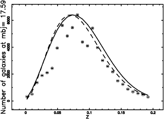
Figure 11: The galaxies of the 2dFGRS database with $16.77\leq bJmag\leq 18.40$ or $4677\frac{L_{\ast{\odot}}}{Mpc^{2}}\leq f\leq 21087\frac{L_{\ast{\odot}}}{Mpc^{2}}$ (with $bJmag$ representing the relative magnitude used in object selection), are isolated in order to represent a chosen value of $m$ and then organized as frequency versus heliocentric redshift, (empty circles); the error bar is given by the square root of the frequency. The maximum in the frequencies of observed galaxies is at $z=0.085$ when $\mathcal{M_{\ast{\odot}}}$ = 5.33 and $h$=1 . The theoretical curve generated by the Schechter function of luminosity (formula (36) and parameters as in column 2dFGRS of Table 5) is drawn (full line). The theoretical curve generated by LF4, formula (42), and parameters as in column 2dFGRS of Table 6) is drawn (dashed line); $\chi^{2}$= 8078 for the Schechter function and $\chi^{2}$= 6654 for LF4.

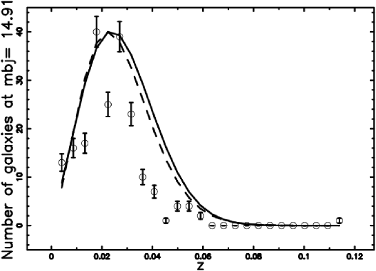
Figure 12: Galaxies in the 2dFGRS with $14.79\leq bJmag\leq 15.02$ or $105142\frac{L_{\ast{\odot}}}{Mpc^{2}}\leq f\leq 129757\frac{L_{\ast{\odot}}}{Mpc^{2}}$. The maximum in the frequencies of observed galaxies is at $z=0.02$, $\mathcal{M_{\ast{\odot}}}$ = 5.33, $\chi^{2}$= 348 for the Schechter function (full line) and $\chi^{2}$= 243 for LF4 (dashed line).

Due to the importance of the maximum as a function of $z$ in the number of galaxies, Figure 13 reports the observed histograms in the 2dFGRS database and the theoretical curves as a function of magnitude.

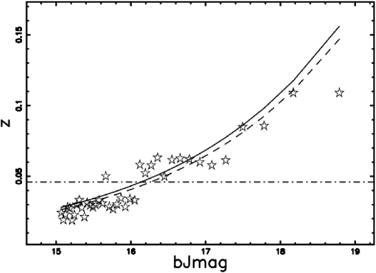
Figure 13: Value of $z$ at which the number of galaxies in the 2dFGRS database is maximum as a function of the apparent magnitude $bJmag$ (stars), theoretical curve of the maximum for the Schechter function as represented by formula (40) (full line) and theoretical curve of the maximum for LF4 as represented by formula (45) (dashed line) when $\mathcal{M_{\ast{\odot}}}$ = 5.33 and $h$=1. The dash-dot-dash horizontal line represents the upper limit of the complete sample.

The total number of galaxies in the 2dFGRS database is reported in Figure 14 as well as the theoretical curves as represented by the numerical integration of formula (36) and formula (42).

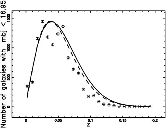
Figure 14: The galaxies in the 2dFGRS database with $13.44\leq bJmag\leq 16.94$ or $17950\frac{L_{\ast{\odot}}}{Mpc^{2}}\leq f\leq 493844\frac{L_{\ast{\odot}}}{Mpc^{2}}$, are organized as frequency versus heliocentric redshift, (empty stars). The theoretical curves generated by the integral of the Schechter function in flux (formula (38) with parameters as in Table 5) (full line) and by the integral of LF4 as represented by formula (43) with parameters as in column 2dFGRS of Table 6) (dashed line) are drawn when $\mathcal{M_{\ast{\odot}}}$ = 5.33 and $h$=1. The numerical analysis gives $\chi^{2}$= 3314 for the Schechter function (full line) and $\chi^{2}$= 2246 for LF4 (dashed line).

Particular attention should be paid to the concept of limiting magnitude and to the corresponding completeness in absolute magnitude of the considered catalogue as a function of redshift. The observable absolute magnitude as a function of the limiting apparent magnitude, $m_{L}$, is

$$M_{L}=m_{{L}}-5\,{\it\log_{10}}\left({\frac{{\it c_{L}}\,z}{H_{{0}}}}\right)-25\quad.$$ (46)

The interval covered by the LF of galaxies, $\Delta M$, is defined as

$$\Delta M=M_{max}-M_{min}\quad,$$ (47)

where $M_{max}$ and $M_{min}$ are the maximum and minimum absolute magnitudes of the LF for the considered catalogue. The real observable interval in absolute magnitude, $\Delta M_{L}$, is

$$\Delta M_{L}=M_{L}-M_{min}\quad.$$ (48)

We can therefore introduce the range of observable absolute maximum magnitude expressed in percent, $\epsilon(z)$, as

$$\epsilon(z)=\frac{\Delta M_{L}}{\Delta M}\times 100\quad.$$ (49)

This is a number that represents the completeness of the sample and can be considered to be a version in percentage terms of the Malmquist bias for the apparent magnitude of a limited number of samples, see [27, 28]. Figure 15 shows the behavior of the range in absolute magnitude in percent as a function of $z$ when the limiting magnitude of 2dFGRS is $m_{L}$=19.61 . From the previous figure, it is possible to conclude that the 2dFGRS catalogue is complete for $z\leq 0.0442$ .

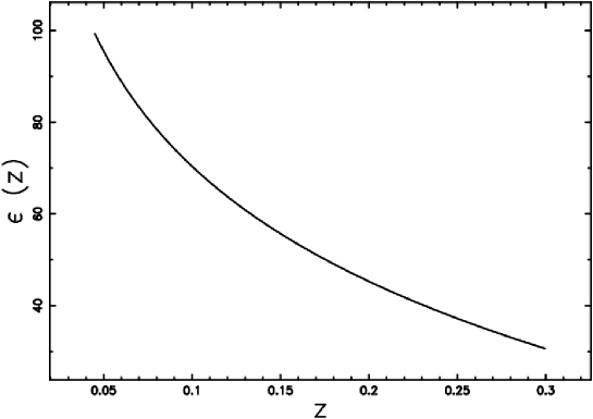
Figure 15: Range in percent of the observable absolute magnitude as a function of the redshift when $M_{max}$=-16, $M_{min}$= -22, $m_{L}$=19.61 and $h$=1.

In this section we have adopted the absolute magnitude of the sun in the $b_{j}$ filter $\mathcal{M_{\ast{\odot}}}$ = 5.33, see [8, 29].

6 Summary

We have presented three new LFs of galaxies based on two different versions of the generalized gamma distribution. Before continuing, we should spend some time discussing the high values of $\chi^{2}$ obtained in Tables 1, 2, 3 and 4. We quote the following phrase from web site http://cosmo.nyu.edu/blanton/lf.html: ”Thus, when comparing to theory it would be totally inappropriate to rely on $\chi^{2}$ from these errors. Such a $\chi^{2}$ will always be very high even for very successful theories.” From the previous statement we can deduce that the high values of $\chi^{2}$ are part of expected results. The reduced values of $\chi_{red}^{2}$ conversely give acceptable results.

From our numerical analysis we draw the following conclusions:

• The generalized gamma galaxy LF with five parameters, formula (16), produces a ”better fit” than the Schechter LF in all five bands considered, see Table 1. As an example, in the $u^{*}$ band, $\chi^{2}$ and $\chi_{red}^{2}$ are 282 and 0.59 against 330 and 0.68 for the Schechter LF.

• The generalized gamma galaxy LF with four parameters, formula (21), produces a ”better fit” than the Schechter LF in all five bands considered, see Table 2. As an example, in the $g^{*}$ band, $\chi^{2}$ and $\chi_{red}^{2}$ are 747 and 1.263 against 753 and 1.263 for the Schechter LF. Because the number of parameters is less, $\chi^{2}$, $AIC$ and $BIC$ are higher than in the case of the generalized gamma galaxy LF with five parameters, see Table 1.

• The LF of galaxies obtained from the generalized gamma PDF for the mass of galaxies assuming $L\propto M^{d}$, formula (28), produces values of $d$ that are slightly greater than one and a ”better fit” than the Schechter LF in all five bands considered, see Table 3. As an example, in the $r^{*}$ band, $\chi^{2}$ and $\chi_{red}^{2}$ are 2217 and 3.31 against 2260 and 3.36 for the Schechter LF.

The Schechter LF of galaxies can also be improved by incorporating a transformation of location, formula (30), and the numerical analysis produces a ”better fit” than the standard Schechter LF in three out of the five bands analyzed, see Table 4. As an example, in the $z^{*}$ band, $\chi^{2}$ and $\chi_{red}^{2}$ are 3133 and 4.25 against 3245 and 4.4 for the Schechter LF.

One of the four new LFs, more precisely the generalized gamma with four parameters, (equation (18)), was tested on the 2dFGRS database and the analysis of $\chi^{2}$ on the histogram of observed frequencies versus redshift produces $\chi^{2}$=6654 for the new LF against $\chi^{2}$=8078 for the Schechter function.

References

• [1] M. S. Longair, Galaxy Formation, Springer, Berlin, 2008.
• [2] P. Padmanabhan, Theoretical astrophysics. Vol. III: Galaxies and Cosmology, Cambridge University Press, Cambridge, MA, 2002.
• [3] J. E. Gunn, M. Carr, C. Rockosi, M. Sekiguchi, K. Berry, B. Elms, E. de Haas, Ž. Ivezić, G. Knapp, R. Lupton, G. Pauls, AJ 116, 3040(1998) .
• [4] P. Schechter, ApJ  203, 297(1976) .
• [5] L. S. Sparke, J. S. Gallagher, Galaxies in the universe : an introduction, Cambridge University Press, Cambridge, UK, 2000.
• [6] S. P. Driver, S. Phillipps, ApJ  469, 529(1996) .
• [7] M. R. Blanton, R. H. Lupton, D. J. Schlegel, M. A. Strauss, J. Brinkmann, M. Fukugita, J. Loveday, ApJ  631, 208(2005) .
• [8] E. Tempel, J. Einasto, M. Einasto, E. Saar, E. Tago, A&A  495, 37(2009) .
• [9] M. Tanemura, Forma 18, 221(2003) .
• [10] A. L. Hinde , R. Miles, J. Stat. Comput. Simul. 10, 205(1980) .
• [11] M. Evans, N. Hastings, B. Peacock, Statistical Distributions - third edition, John Wiley & Sons Inc, New York, 2000.
• [12] M. R. Blanton, D. W. Hogg, N. A. Bahcall, J. Brinkmann, M. Britton, ApJ  592, 819(2003) .
• [13] H. Lin, R. P. Kirshner, S. A. Shectman, S. D. Landy, A. Oemler, D. L. Tucker, P. L. Schechter, ApJ  464, 60(1996) .
• [14] J. Machalski, W. Godlowski, A&A  360, 463(2000) .
• [15] W. H. Press, S. A. Teukolsky, W. T. Vetterling, B. P. Flannery, Numerical recipes in FORTRAN. The art of scientific computing, Cambridge University Press, Cambridge, 1992.
• [16] H. Akaike, IEEE Transactions on Automatic Control 19, 716(1974) .
• [17] A. R. Liddle, MNRAS  351, L49(2004) .
• [18] W. Godlowski, M. Szydowski, Constraints on Dark Energy Models from Supernovae, in: M. Turatto, S. Benetti, L. Zampieri, W. Shea (Eds.), 1604-2004: Supernovae as Cosmological Lighthouses, Vol. 342 of Astronomical Society of the Pacific Conference Series, 2005, 508–+.
• [19] G. Schwarz, Annals of Statistics 6, 461(1978) .
• [20] M. R. Blanton, J. Dalcanton, D. Eisenstein, J. Loveday, M. A. Strauss, M. SubbaRao, D. H. Weinberg, J. E. Anderson, J. Annis, N. A. Bahcall, M. Bernardi, J. Brinkmann, R. J. Brunner, AJ 121, 2358(2001) .
• [21] L. Zaninetti, AJ 135, 1264(2008) .
• [22] T. Kiang, Z. Astrophys. 64, 433(1966) .
• [23] L. Zaninetti, Acta Physica Polonica B 39, 1467(2008) .
• [24] T. Padmanabhan, Cosmology and Astrophysics through Problems, Cambridge University Press, Cambridge, 1996.
• [25] M. Colless, G. Dalton, S. Maddox, et al., MNRAS  328, 1039(2001) .
• [26] D. S. Madgwick, O. Lahav, I. K. Baldry, C. M. Baugh, J. Bland-Hawthorn, T. Bridges, MNRAS  333, 133(2002) .
• [27] K. Malmquist , Lund Medd. Ser. II 22, 1(1920) .
• [28] K. Malmquist , Lund Medd. Ser. I 100, 1(1922) .
• [29] V. R. Eke, C. S. Frenk, C. M. Baugh, S. Cole, P. Norberg, MNRAS  355, 769(2004) .