Solution of the tunneling-percolation problem in the nanocomposite regime

Abstract

We noted that the tunneling-percolation framework is quite well understood at the extreme cases of percolation-like and hopping-like behaviors but that the intermediate regime has not been previously discussed, in spite of its relevance to the intensively studied electrical properties of nanocomposites. Following that we study here the conductivity of dispersions of particle fillers inside an insulating matrix by taking into account explicitly the filler particle shapes and the inter-particle electron tunneling process. We show that the main features of the filler dependencies of the nanocomposite conductivity can be reproduced without introducing any a priori imposed cut-off in the inter-particle conductances, as usually done in the percolation-like interpretation of these systems. Furthermore, we demonstrate that our numerical results are fully reproduced by the critical path method, which is generalized here in order to include the particle filler shapes. By exploiting this method, we provide simple analytical formulas for the composite conductivity valid for many regimes of interest. The validity of our formulation is assessed by reinterpreting existing experimental results on nanotube, nanofiber, nanosheet and nanosphere composites and by extracting the characteristic tunneling decay length, which is found to be within the expected range of its values. These results are concluded then to be not only useful for the understanding of the intermediate regime but also for tailoring the electrical properties of nanocomposites.

I Introduction

The inclusion of nanometric conductive fillers such as carbon nanotubes Bauhofer2009 , nanofibers Al-Saleh2009 , and graphene Eda2009 ; Stankovich2006 into insulating matrices allows to obtain electrically conductive nanocomposites with unique properties which are widely investigated and have several technological applications ranging from antistatic coatings to printable electronics Sekitani2009 . A central challenge in this domain is to create composites with an overall conductivity $\sigma$ that can be controlled by the volume fraction $\phi$, the shape of the conducting fillers, their dispersion in the insulating matrix, and the local inter-particle electrical connectedness. Understanding how these local properties affect the composite conductivity is therefore the ultimate goal of any theoretical investigation of such composites.

A common feature of most random insulator-conductor mixtures is the sharp increase of $\sigma$ once a critical volume fraction $\phi_{c}$ of the conductive phase is reached. This transition is generally interpreted in the framework of percolation theory Kirkpatrick1973 ; Stauffer1994 ; Sahimi2003 and associated with the formation of a cluster of electrically connected filler particles that spans the entire sample. The further increase of $\sigma$ for $\phi>\phi_{c}$ is likewise understood as the growing of such a cluster. In the vicinity of $\phi_{c}$, this picture implies a power-law behavior of the conductivity of the form

$$\sigma\propto(\phi-\phi_{c})^{t},$$ (1)

where $t$ is a critical exponent. Values of $t$ extracted from experiments range from its expected universal value for three-dimensional percolating systems, $t\simeq 2$, up to $t\simeq 10$, with little or no correlation to the critical volume fraction $\phi_{c}$,Vionnet2005 or the shape of the conducting fillers Bauhofer2009 .

In the dielectric regime of a system of nanometric conducting particles embedded in a continuous insulating matrix, as is the case for conductor-polymer nano-composites,Sheng1978 ; Balberg1987b ; Paschen1995 ; Li2007 the particles do not physically touch each other, and the electrical connectedness is established through tunneling between the conducting filler particles. In this situation, the basic assumptions of percolation theory are, a priori, at odds with the inter-particle tunneling mechanism.Balberg2009 Indeed, while percolation requires the introduction of some sharp cut-off in the inter-particle conductances, i.e., the particles are either connected (with given non-zero inter-particle conductances) or disconnected,Stauffer1994 ; Sahimi2003 the tunneling between particles is a continuous function of inter-particle distances. Hence, the resulting tunneling conductance, which decays exponentially with these distances, does not imply any sharp cut-off or threshold.

Quite surprisingly, this fundamental incompatibility has hardly been discussed in the literature,Balberg2009 and basically all the measured conductivity dependencies on the fractional volume content of the conducting phase, $\sigma(\phi)$, have been interpreted in terms of Eq. (1) assuming the “classical” percolation behavior.Stauffer1994 ; Sahimi2003 In this article, we show instead that the inter-particle tunneling explains well all the main features of $\sigma(\phi)$ of nanocomposites without imposing any a priori cut-off, and that it provides a much superior description of $\sigma(\phi)$ than the “classical” percolation formula (1).

In order to specify our line of reasoning and to better appreciate the above mentioned incompatibility, it is instructive to consider a system of particle dispersed in an insulating continuum with a tunneling conductance between two of them, $i$ and $j$, given by:

$$g_{ij}=g_{0}\exp\!\left(-\frac{2\delta_{ij}}{\xi}\right),$$ (2)

where $g_{0}$ is a constant, $\xi$ is the characteristic tunneling length, and $\delta_{ij}$ is the minimal distance between the two particle surfaces. For spheres of diameter $D$, $\delta_{ij}=r_{ij}-D$ where $r_{ij}$ is the center-to-center distance. There are two extreme cases for which the resulting composite conductivity has qualitatively different behaviors which can be easily described. In the first case the particles are so large that $\xi/D\rightarrow 0$. It becomes then clear from Eq.(2) that the conductance between two particles is non-zero only when they essentially touch each other. Hence, removing particles from the random closed packed limit is equivalent to remove tunneling bonds from the system, in analogy to sites removal in a site percolation problem in the lattice.Stauffer1994 ; Sahimi2003 The system conductivity will have then a percolation-like behavior as in Eq. (1) with $t\simeq 2$ and $\phi_{c}$ being the corresponding percolation threshold.Johner2008 The other extreme case is that of sites ($D/\xi\rightarrow 0$) randomly dispersed in the continuum. In this situation, a variation of the site density $\rho$ does not change the connectivity between the particles and its only role is to vary the distances $\delta_{ij}=r_{ij}$ between the sites.Balberg2009 ; Shklovskii1984 The corresponding $\sigma$ behavior was solved by using the critical path (CP) methodAmbegaokar1971 in the context of hopping in amorphous semiconductors yielding $\sigma\propto\exp[-1.75/(\xi\rho^{1/3})]$.Seager1974 ; Overhof1989 For sufficiently dilute system of impenetrable spheres this relation can be generalized to $\sigma\propto\exp[-1.41D/(\xi\phi^{1/3})]$.Balberg2009 It is obvious then from the above discussion that the second case is the low density limit of the first one, but it turns out that the variation of $\sigma(\phi)$ between the two types of situations, which is definitely pertinent to nanocomposites, has not been studied thus far.

Following the above considerations we turned to study here the $\sigma(\phi)$ dependencies by extending the low-density (hopping-like) approach to higher densities than those used previously.Shklovskii1984 ; Seager1974 ; Overhof1989 Specifically, we shall present numerical results obtained by using the global tunneling network (GTN) model, where the conducting fillers form a network of globally connected sites via tunneling processes. This model has already been introduced in Ref.[Ambrosetti2009, ] for the case of impenetrable spheres, but here we shall generalize it in order to describe also anisotropic fillers such as rod-like and plate-like particles, as to apply to cases of recent interest (i.e., nanotube, nanofiber, nanosheet, and graphene composites). In particular, the large amount of published experimental data on these systems allows us to test the theory and to extract the values of microscopic parameters directly from macroscopic data on the electrical conductivity.

The structure of the paper is as follows. In Sec. II we describe how we generate particle dispersions and in Sec. III we calculate numerically the composite conductivities within the GTN model and compare them with the conductivities obtained by the CP approximation. In Sec. IV we present our results on the critical tunneling distance which are used in Sec. V to obtain analytical formulas for the composite conductivity. These are applied in Sec. VI to several published data on nanocomposites to extract the tunneling distance. Section VII is devoted to discussions and conclusions.

II sample generation

In modeling the conductor-insulator composite morphology, we treat the conducting fillers as identical impenetrable objects dispersed in a continuous insulating medium, with no interactions between the conducting and insulating phases. As pointed out above, in order to relate to systems of recent interest we describe filler particle shapes that vary from rod-like (nanotubes) to plate-like (graphene). This is done by employing impenetrable spheroids (ellipsoids of revolution) ranging from the extreme prolate ($a/b\gg 1$) to the extreme oblate limit ($a/b\ll 1$), where $a$ and $b$ are the spheroid polar and equatorial semi-axes respectively.

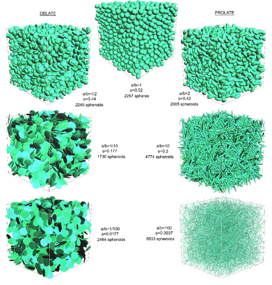
Figure 1: (Color online) Examples of distributions of impenetrable spheres and spheroids of different aspect-ratios $a/b$ and volume fraction $\phi$ generated by the algorithms used in the present work.

We generate dispersions of non-overlapping spheroids by using an extended version of a previously described algorithmAmbrosetti2008 which allows to add spheroids into a cubic cell with periodic boundary conditions through random sequential addition (RSA).Sherwood1997 Since the configurations obtained via RSA are non-equilibrium ones,Torquato2001 ; Miller2009 the RSA dispersions were relaxed via Monte Carlo (MC) runs, where for each spheroid a random displacement of its center and a random rotation of its axes Frenkel1985 were attempted, being accepted only if they did not give rise to an overlap with any of its neighbors. Equilibrium was considered attained when the ratio between the number of accepted trial moves versus the number of rejected ones had stabilized. Furthermore, to obtain densities beyond the ones obtainable with RSA, a high density generation procedure Ambrosetti2009 ; Miller1990 was implemented where in combination with MC displacements the particles were also inflated. The isotropy of the distributions was monitored by using the nematic order parameter as described in Ref.[Schilling2007, ].

Figure 1 shows examples of the so-generated distributions for spheroids with different aspect-ratios $a/b$ and volume fractions $\phi=V\rho$, where $V=4\pi ab^{2}/3$ is the volume of a single spheroid and $\rho$ is the particle number density.

III determination of the composite conductivity by the GTN and CP methods

In considering the overall conductivity arising in such composites, we attributed to each spheroid pair the tunneling conductance given in Eq. (2) where, now, for $a/b\neq 1$ the inter-particle distance $\delta_{ij}$ depends also on the relative orientation of the spheroids. The $\delta_{ij}$ values were obtained here from the numerical procedure described in Ref.[Ambrosetti2008, ]. On the other hand, in writing Eq. (2) we neglect any energy difference between spheroidal particles and disregard activation energies since, in general, these contributions can be ignored at relatively high temperatures,Shklovskii1984 ; Sheng1983 which is the case of interest here. For the specific case of extreme prolate objects ($a/b\gg 1$) the regime of validity of this approximation has been studied in Ref.[Hu2006, ].

The full set of bond conductances given by Eq. (2) was mapped as a resistor network with $g_{0}=1$ and the overall conductivity was calculated through numerical decimation of the resistor network.Johner2008 ; Fogelholm1980 To reduce computational times of the decimation procedure to manageable limits, an artificial maximum distance was introduced in order to reject negligibly small bond conductances. It is important to note that this artifice is not in conflict with the rationale of the GTN model, since the cutoff it implies neglects conductances which are completely irrelevant for the global system conductivity. We chose the maximum distance to be generally fixed and equal to four times the spheroid major axis (i.e. $a$ in the prolate case and $b$ in the oblate case), which is equivalent to reject inter-particle conductances below $e^{-60}$ for $\xi/D=1/15$ case (and considerably less for smaller $\xi$ values). However, for the high aspect-ratios and high densities the distance had to be reduced. Moreover, since the maximum distance implies in turn an artificial geometrical percolation threshold of the system, for the high aspect-ratios, at low volume fractions the distance had to be increased to avoid this effect. By comparing the results with the ones obtained with significantly larger maximum distances we verified that the effect is undetectable.

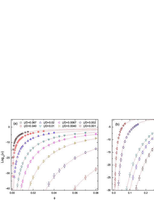
Figure 2: (Color online) The results of our GTN and CP calculations. (a): Volume fraction $\phi$ dependence of the tunneling conductivity $\sigma$ for a system of aspect-ratio $a/b=10$ hard prolate spheroids with different characteristic tunneling distances $\xi/D$ with $D=2a$. Results from Eq. (3) (with $\sigma_{0}=0.179$) are displayed by dotted lines. (b): Tunneling conductivity in a system of hard spheroids with different aspect-ratios $a/b$ and $\xi/D=0.01$, with $D=2\max(a,b)$. Dotted lines: results from Eq. (3) with $\sigma_{0}=0.124$ for $a/b=2$, $\sigma_{0}=0.099$ for $a/b=1/2$, $\sigma_{0}=0.351$ for $a/b=1/10$, and $\sigma_{0}=0.115$ for $a/b=1$.

In Fig. 2(a) we show the so-obtained conductivity $\sigma$ values (symbols) as a function of the volume fraction $\phi$ of prolate spheroids with aspect-ratio $a/b=10$ and different values of $\xi/D$, where $D=2\max(a,b)$. Each symbol is the outcome of $N_{R}=200$ realizations of a system of $N_{P}\sim 1000$ spheroids. The logarithm average of the results was considered since, due to the exponential dependence of Eq. (2), the distribution of the computed conductivities was approximately of the log-normal form.Strelniker2005 The strong reduction of $\sigma$ for decreasing $\phi$ shown in Fig. 2(a) is a direct consequence of the fact that as $\phi$ is reduced, the inter-particle distances get larger, leading in turn to a reduction of the local tunneling conductances [Eq. (2)]. In fact, as shown in Fig. 2(b), this reduction depends strongly on the shape of the conducting fillers. Specifically, as the shape anisotropy of the particles is enhanced, the composite conductivity drops for much lower values of $\phi$ for a fixed $\xi$.

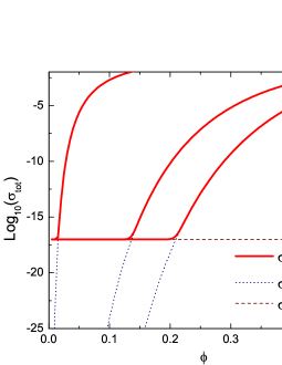
Figure 3: (Color online) Schematic illustration of the tunneling conductivity crossover for the cases $a/b=1$, $a/b=2$, and $a/b=10$.

Having the above result we turn now to show that the strong dependence of $\sigma(\phi)$ on $a/b$ and $\xi$ in Fig. 2 can be reproduced by CP method Shklovskii1984 ; Ambegaokar1971 ; Seager1974 ; Overhof1989 when applied to our system of impenetrable spheroids. For the tunneling conductances of Eq. (2), this method amounts to keep only the subset of conductances $g_{ij}$ having $\delta_{ij}\leq\delta_{c}$, where $\delta_{c}$, which defines the characteristic conductance $g_{c}=g_{0}\exp(-2\delta_{c}/\xi)$, is the largest among the $\delta_{ij}$ distances, such that the so-defined subnetwork forms a conducting cluster that span the sample. Next, by assigning $g_{c}$ to all the (larger) conductances of the subnetwork, a CP approximation for $\sigma$ is

$$\sigma\simeq\sigma_{0}\exp\left[-\frac{2\delta_{c}(\phi,a,b)}{\xi}\right],$$ (3)

where $\sigma_{0}$ is a pre-factor proportional to $g_{0}$. The significance of Eq. (3) is that it reduces the conductivity of a distribution of hard objects that are electrically connected by tunneling to the computation of the geometrical “critical” distance $\delta_{c}$. In practice, $\delta_{c}$ can be obtained by coating each impenetrable spheroid with a penetrable shell of constant thickness $\delta/2$, and by considering two spheroids as connected if their shells overlap. $\delta_{c}$ is then the minimum value of $\delta$ such that, for a given $\phi$, a cluster of connected spheroids spans the sample.

To extract $\delta_{c}$ we follow the route outlined in Ref. [Ambrosetti2008, ] with the extended distribution generation algorithm described in Sec. II. Specifically, we calculated the spanning probability as a function of $\phi$ for fixed $a/b$ and $\delta_{c}$ by recording the frequency of appearance of a percolating cluster over a given number of realizations $N_{R}$. The realization number varied from $N_{R}=40$ for the smallest values of $\delta_{c}$ up to $N_{R}=500$ for the largest ones. Each realization involved distributions of $N_{P}\sim 2000$ spheroids, while for high aspect-ratio prolate spheroids this number increased to $N_{P}\sim 8000$ in order to be able to maintain the periodic boundary conditions on the simulation cell. Relative errors on $\delta_{c}$ were in the range of a few per thousand.

Results of the CP approximation are reported in Fig. 2 by dotted lines. The agreement with the full numerical decimation of the resistor network is excellent for all values of $a/b$ and $\xi/D$ considered. This observation is quite important since it shows that the CP method is valid also beyond the low-density regime, for which the conducting fillers are effectively point particles, and that it can be successfully used for systems of particles with impenetrable volumes. Besides the clear practical advantage of evaluating $\sigma$ via the geometrical quantity $\delta_{c}$ instead of solving the whole resistor network, the CP approximation is found then, as we shall see in the next section, to allow the full understanding of the filler dependencies of $\sigma$ and to identify asymptotic formulas for many regimes of interest.

Before turning to the analysis of the next section, it is important at this point to discuss the following issue. As shown in Fig. 2, the GTN scenario predicts, in principle, an indefinite drop of $\sigma$ as $\phi\rightarrow 0$ because, by construction, there is not an imposed cut-off in the inter-particle conductances. However, in real composites, either the lowest measurable conductivity is limited by the experimental set-up,Balberg2009 or it is given by the intrinsic conductivity $\sigma_{\rm m}$ of the insulating matrix, which prevents an indefinite drop of $\sigma$. For example, in polymer-based composites $\sigma_{\rm m}$ falls typically in the range of $\sigma_{\rm m}\simeq 10^{-13}\div 10^{-18}$ S/cm, and it originates from ionic impurities or displacement currents.Blyte2005 Since the contributions from the polymer and the inter-particle tunneling come from independent current paths, the total conductivity (given by the polymer and the inter-particle tunneling) is then simply $\sigma_{\rm tot}=\sigma_{\rm m}+\sigma$.notecross As illustrated in Fig. 3, where $\sigma_{\rm tot}$ is plotted for $a/b=1$, $2$, and $10$ and for $\sigma_{\rm m}/\sigma_{0}=10^{-17}$, the $\phi$-dependence of $\sigma_{\rm tot}$ is characterized by a cross-over concentration $\phi_{c}$ below which $\sigma_{\rm tot}\simeq\sigma_{\rm m}$. As seen in this figure, fillers with larger shape-anisotropy entail lower values of $\phi_{c}$, consistently with what is commonly observed.Bauhofer2009 ; Ota1997 ; Nagata1999 ; Lu2006 We have therefore that the main features of nanocomposites (drop of $\sigma$ for decreasing $\phi$, enhancement of $\sigma$ at fixed $\phi$ for larger particle anisotropy, and a characteristic $\phi_{c}$ below which the conductivity matches that of the insulating phase) can be obtained without invoking any microscopic cut-off, leading therefore to a radical change of perspective from the classical percolation picture. In particular, in the present context, the conductor-insulator transition is no longer described as a true percolation transition (characterized by a critical behavior of $\sigma$ in the vicinity of a definite percolation threshold, i.e., Eq.(1)), but rather as a cross-over between the inter-particle tunneling conductivity and the insulating matrix conductivity.

IV CP determination of the critical distance $\delta_{c}$ for spheroids

The importance of the CP approximation for the understanding of the filler dependencies of $\sigma$ is underscored by the fact that, as discussed below, for sufficiently elongated prolate and for sufficiently flat oblate spheroids, as well as for spheres, simple relations exist that allow to estimate the value of $\delta_{c}$ with good accuracy. In virtue of Eq. (3) this means that we can formulate explicit relations between $\sigma$ and the shapes and concentration of the conducting fillers.

IV.1 prolate spheroids

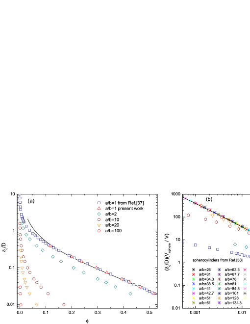
Figure 4: (Color online) (a): the $\delta_{c}/D$ dependence on the volume fraction $\phi$ for impenetrable prolate spheroids with $a/b=1$, $2$, $10$, $20$, and $100$. For $a/b=1$ our results are plotted together with those of Ref. [Heyes2006, ]. The solid line is Eq. (9). (b): re-scaled critical distances versus $\phi$ for prolate spheroids as well as for the impenetrable spherocylinders of Refs. [Schilling2007, ; Berhan2007, ]. The dashed line follows Eq. (4) and the solid line follows Eq. (5)

Let us start with prolate ($a/b>1$) spheroids. In Fig. 4(a) we present the calculated values of $\delta_{c}/D$ as a function of the volume fraction $\phi$ for spheres ($a/b=1$, together with the results of Ref. [Heyes2006, ]) and for $a/b=2$, $10$, $20$, and $100$. In the log-log plot of Fig. 4(b) the same data are displayed with $\delta_{c}/D$ multiplied by the ratio $V_{\rm sphere}/V=(a/b)^{2}$, where $V_{\rm sphere}=\pi D^{3}/6$ is the volume of a sphere with diameter equal to the major axis of the prolate spheroid and $V=4\pi ab^{2}/3$ is the volume of the spheroid itself. For comparison, we also plot in Fig. 4(b) the results for impenetrable spherocylinders of Refs. [Schilling2007, ; Berhan2007, ]. These are formed by cylinders of radius $R$ and length $L$, capped by hemispheres of radius $R$, so that $a=R+L/2$ and $b=R$, and $V_{\rm sphere}/V=(a/b)^{3}/[(3/2)(a/b)-2]\simeq(2/3)(a/b)^{2}$ for $a/b\gg 1$. As it is apparent, for sufficiently large values of $a/b$ the simple re-scaling transformation collapses both spheroids and spherocylinders data into a single curve. This holds true as long as the aspect-ratio of the spheroid plus the penetrable shell $(a+\delta_{c}/2)/(b+\delta_{c}/2)$ is larger than about $5$. In addition, for $\phi\lesssim 0.03$ the collapsed data are well approximated by $\delta_{c}V_{\rm sphere}/V/D=0.4/\phi$ [dashed line in Fig. 4(b)], leading to the following asymptotic formula:

$$\delta_{c}/D\simeq\frac{\gamma(b/a)^{2}}{\phi},$$ (4)

where $\gamma=0.4$ for spheroids and $\gamma=0.6$ for spherocylinders. Equation (4) is fully consistent with the scaling law of Ref. [Kyrylyuk2008, ] that was obtained from the second-virial approximation for semi-penetrable spherocylinders, and it can be understood from simple excluded volume effects. Indeed, in the asymptotic regime $a/b\gg 1$ and for $\delta_{c}/a\ll 1$, the filler density $\rho$ (such that a percolating cluster of connected semi-penetrable spheroids with penetrable shell $\delta_{c}$ is formed) is given by $\rho=1/\Delta V_{\rm exc}$.Berhan2007 ; Balberg1984 ; Bug1986 Here, $\Delta V_{\rm exc}$ is the excluded volume of a randomly oriented semi-penetrable object minus the excluded volume of the impenetrable object. As shown in the Appendix, for both spheroids and spherocylinder particles this becomes $\Delta V_{\rm exc}\simeq 2\pi a^{2}\delta_{c}$, leading therefore to Eq. (4) with $\gamma=1/3$ for spheroids and $\gamma=1/2$ for spherocylinders.noteshoot

It is interesting to notice that in Fig. 4(b) the re-scaled data for $\phi\gtrsim 0.03$ deviate from Eq. (4) but still follow a common curve. We have found that this common trend is well fitted by an empirical generalization of Eq. (4):

$$\delta_{c}/D\simeq\frac{\gamma(b/a)^{2}}{\phi(1+8\phi)},$$ (5)

which applies to all values of $\phi$ provided that $(a+\delta_{c}/2)/(b+\delta_{c}/2)\gtrsim 5$ [solid lines in Fig. 4(b)].

IV.2 oblate spheroids

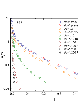
Figure 5: (Color online) (a): the $\delta_{c}/D$ dependence on the volume fraction $\phi$ for impenetrable oblate spheroids with $a/b=1$, $1/2$, $1/10$, $1/100$, and $1/200$. Results obtained by RSA alone are also presented. (b): our $\delta_{c}/D$ values plotted versus the re-scale volume fraction $\phi(b/a)$. The dashed line follows Eq. (6) and the solid line follows Eq. (7). Inset: the asymptotic behavior for $\delta_{c}/D<0.1$.

Let us now turn to the case of oblate spheroids. The numerical results for $\delta_{c}$ as a function of the volume fraction $\phi$ are displayed in Fig. 5(a) for $a/b=1$, $1/2$, $1/10$, $1/100$, and $1/200$. Now, as opposed to prolate fillers, almost all of the experimental results on nanocomposites, such as graphene,Stankovich2006 that contain oblate filler with high shape anisotropy are at volume fractions for which a corresponding hard spheroid fluid at equilibrium would already be in the nematic phase. For oblate spheroids with $a/b=1/10$ the isotropic-nematic (I-N) transition is at $\phi_{\rm I-N}\sim 0.185$,Allen1989 while for lower $a/b$ values the transition may be estimated from the results on infinitely thin hard disks:Eppenga1984 $\phi_{\rm I-N}\sim 0.0193$ for $a/b=1/100$ and $\phi_{\rm I-N}\sim 0.0096$ for $a/b=1/200$. However, in real nanocomposites the transition to the nematic phase is hampered by the viscosity of the insulating matrix and these systems are inherently out of equilibrium.kharchenko In order to maintain global isotropy also for $\phi>\phi_{\rm I-N}$, we generated oblate spheroid distributions with RSA alone. The outcomes are again displayed in Fig. 5 and one can appreciate that the difference with the equilibrium results for $\phi<\phi_{\rm I-N}$ is quite small and negligible for the present aims.

In analogy to what we have done for the case of prolate objects, it would be useful to find a scaling relation permitting to express the $\phi$-dependence of $\delta_{c}/D$ also for oblate spheroids, at least for the $a/b\ll 1$ limit, which is the one of practical interest. To this end, it is instructive to consider the case of perfectly parallel spheroids which can be easily obtained from general result for aligned penetrable objects.Balberg1985 For infinitely thin parallel hard disks of radius $b$ one therefore has $V_{\rm exc}^{\|}=2.8/\rho$, where $V_{\rm exc}^{\|}=(4/3)\pi b^{3}[12(\delta_{c}/D)+6\pi(\delta_{c}/D)^{2}+8(\delta_{c}/D)^{3}]$ is the excluded volume of the plate plus the penetrable shell of critical thickness $\delta_{c}/2$. Assuming that this holds true also for hard-core-penetrable-shell oblate spheroids with a sufficiently thin hard core, we can then write

$$12(\delta_{c}/D)+6\pi(\delta_{c}/D)^{2}+8(\delta_{c}/D)^{3}\simeq\frac{2.8}{\phi(b/a)},$$ (6)

which implies that $\delta_{c}/D$ depends solely on $\phi(b/a)$. As shown in the Appendix, where the excluded volume of an isotropic orientation of oblate spheroids is reported, also the second-order virial approximation gives $\delta_{c}/D$ as a function of $\phi(a/b)$ for $a/b\ll 1$. Hence, although Eq. (6) and Eq. (29) are not expected to be quantitatively accurate, they suggest nevertheless a possible way of rescaling the data of Fig. 5(a). Indeed, as shown in Fig. 5(b), for sufficiently high shape anisotropy the data of $\delta_{c}/D$ plotted as a function of $\phi(a/b)$ collapse into a single curve (the results for $a/b=1/100$ and $a/b=1/200$ are completely superposed). Compared to Eq. (6), which behaves as $\delta_{c}/D\propto[\phi(b/a)]^{-1}$ for $\delta_{c}/D\ll 1$ (dashed line), the re-scaled data in the log-log plots of Fig. 5(b) still follow a straight line in the same range of $\delta_{c}/D$ values but with a slightly sharper slope, suggesting a power-law dependence on $\phi(a/b)$. Empirically, Eq. (6) does indeed reproduce then the $a/b\ll 1$ asymptotic behavior by simply modifying the small $\delta_{c}/D$ behavior as follows:

$$12\alpha(\delta_{c}/D)^{\beta}+6\pi(\delta_{c}/D)^{2}+8(\delta_{c}/D)^{3}\simeq\frac{2.8}{\phi(b/a)},$$ (7)

where $\alpha=1.54$ and $\beta=3/4$. When plotted against our data, Eq. (7) (solid line) provides an accurate approximation for $\delta_{c}/D$ in the whole range of $\phi(a/b)$ for $a/b<1/100$. Moreover, by retaining the dominant contribution of Eq. (7) for $\delta_{c}/D<0.1$, we arrive at (inset of Fig. 5(b):

$$\delta_{c}/D\simeq\left[\frac{0.15(a/b)}{\phi}\right]^{4/3},$$ (8)

which applies to all cases of practical interest for plate-like filler particles ($a/b\ll 1$ and $\delta_{c}/D\ll 1$).

IV.3 spheres

Let us conclude this section by providing an accurate expression for $\delta_{c}/D$ also for the case of spherical impenetrable particles. In real homogeneous composites with filler shapes assimilable to spheres of diameter in the sub-micron range, the cross-over volume fraction $\phi_{c}$ is consistently larger than about $0.1$,Ambrosetti2009 so that a formula for $\delta_{c}/D$ that is useful for real nanosphere composites must be accurate in the $\phi\gtrsim 0.1$ range. For these $\phi$ values the scaling relation $\delta_{c}/D\propto\phi^{-1/3}$, which stems by assuming very dilute systems such that $\delta_{c}/D\gg 1$, is of course no longer valid. However, as noticed in Ref. [Johner2008, ], the ratio $\delta_{c}/\delta_{\rm NN}$, where $\delta_{\rm NN}$ is the mean minimal distance between nearest-neighbours spheres, has a rather weak dependence on $\phi$. In particular, we have found that the $\delta_{c}$ data for $a/b=1$ in Fig. 4 are well fitted by assuming that $\delta_{c}=1.65\delta_{\rm NN}$ for $\phi\gtrsim 0.1$. An explicit formula can then be obtained by using the high density asymptotic expression for $\delta_{\rm NN}$ as given in Ref. [Torquato2001, ]. This leads to:

$$\delta_{c}/D\simeq\frac{1.65(1-\phi)^{3}}{12\phi(2-\phi)},$$ (9)

which is plotted by the solid line in Fig. 4(a).

V analytic determination of the filler dependencies of the conductivity

With the results of the previous section, we are now in a position to provide tunneling conductivity formulas of random distributions of prolate, oblate and spherical objects for $\sigma>\sigma_{\rm m}$, where $\sigma_{\rm m}$ is the intrinsic conductivity of the matrix. Indeed, by substituting Eqs. (4), (8), and (9) into Eq. (3) we obtain

$$\sigma\simeq\sigma_{0}\exp\!\left[-\frac{2D}{\xi}\frac{\gamma(b/a)^{2}}{\phi}\right]\,\,\,\textrm{for prolates},$$ (10)

$$\sigma\simeq\sigma_{0}\exp\!\left\{-\frac{2D}{\xi}\left[\frac{0.15(a/b)}{\phi}\right]^{4/3}\right\}\,\,\,\textrm{for oblates},$$ (11)

$$\sigma\simeq\sigma_{0}\exp\!\left[-\frac{2D}{\xi}\frac{1.65(1-\phi)^{3}}{12\phi(2-\phi)}\right]\,\,\,\textrm{for spheres}.$$ (12)

From the previously discussed conditions on the validity of the asymptotic formulas for $\delta_{c}/D$ it follows that the above equations will hold when $(b/a)^{2}\lesssim\phi\lesssim 0.03$ for prolates, $\phi\gtrsim a/b$ and $a/b<0.1$ for oblates, and $\phi\gtrsim 0.1$ for spheres. We note in passing that for the case of prolate objects, a relation of more general validity than Eq. (10) can be obtained by substituting Eq. (5) into Eq. (3).

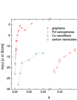
Figure 6: (Color online) (a): natural logarithm of the conductivity $\sigma$ as a function of the volume fraction $\phi$ for different polymer nanocomposites: Graphene-polystyrene,Stankovich2006 Pd nanospheres-polystyrene,Kubat1993 Cu nanofibers-polystyrene,Gelves2006 and single-wall carbon nanotubes-epoxy.Bryning2005 When, for a given concentration, more then one value of $\sigma$ was given (as in Refs. [Gelves2006, ; Bryning2005, ]), the average of $\ln(\sigma)$ was considered. (b), the same data of (a) re-plotted as function of the corresponding critical distance $\delta_{c}$. Solid lines are fits to Eq. (15).

Although we are not aware of previous results on $\sigma$ for dispersions of oblate (plate-like) particles, there exist nevertheless some results for prolate and spherical particles in the recent literature. In Ref. [Hu2006, ], for example, approximate expressions for $\sigma$ for extreme prolate ($a/b\gg 1$) objects and their temperature dependence have been obtained by following the critical path method employed here. It turns out that the temperature independent contribution to $\sigma$ that was given in Ref. [Hu2006, ] has the same dependence on the particle geometry and density of Eq. (10), but without the numerical coefficients. The case of relatively high density spheres has been considered in Ref. [Balberg2009, ] where $\ln(\sigma)\propto 1/\phi$ has been proposed. This implies that $\delta_{c}/D\propto 1/\phi$, which does not adequately fit the numerical results of $\delta_{c}/D$, while Eq. (9), and consequently Eq. (12), are rather accurate for a wide range of $\phi$ values.

In addition to the $\phi$-dependence of the tunneling contribution to the conductivity, Eqs. (10)-(12) provide also estimations for the cross-over value $\phi_{c}$, below which the conductivity basically coincides with the conductivity $\sigma_{\rm m}$ of the insulating matrix. As discussed in Sec.III, and as illustrated in Fig. 3, $\phi_{c}$ may be estimated by the $\phi$ value such that $\sigma\simeq\sigma_{\rm m}$, which leads to

$$\phi_{c}\simeq\frac{2D}{\xi}\frac{\gamma(b/a)^{2}}{\ln(\sigma_{0}/\sigma_{\rm m})},$$ (13)

for prolate and

$$\phi_{c}\simeq 0.15(a/b)\left[\frac{2D}{\xi}\frac{1}{\ln(\sigma_{0}/\sigma_{\rm m})}\right]^{3/4},$$ (14)

for oblate objects. For the case of spheres, $\phi_{c}$ is the root of a third-order polynomial equation. Equations (13) and (14), by construction, display the same dependence on the aspect-ratio of the corresponding geometrical percolation critical densities, as it can be appreciated by comparing them with Eq. (4) (prolates) or with the inverse of Eq. (8) (oblates). However they also show that the cross-over point depends on the tunneling decay length and on the intrinsic matrix conductivity. This implies that if, by some means, one could alter $\sigma_{\rm m}$ in a given composites without seriously affecting $\xi$ and $\sigma_{0}$, then a change in $\phi_{c}$ is to be expected.

VI comparison with experimental data

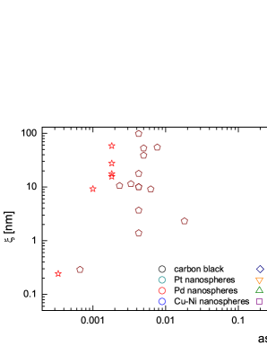
Figure 7: (Color online) Characteristic tunneling distance $\xi$ values for different polymer nanocomposites as extracted form Eq. (15) applied to the data of Refs. [Kubat1993, ; nanosph, ] (low structured carbon black and metallic nanosphere composites), Refs. [Gelves2006, ; Bryning2005, ; nanopro, ] (nanofiber and carbon nanotube composites), and Refs. [Stankovich2006, ; Lu2006, ; nanoobl, ] (nanographite and graphene composites).

In this section we show how the above outlined formalism may be used to re-interpret the experimental data on the conductivity of different nanocomposites that were reported in the literature. In Fig. 6(a) we show the measured data of $\ln(\sigma)$ versus $\phi$ for polymer composites filled with graphene sheets,Stankovich2006 Pd nanospheres,Kubat1993 Cu nanofibers,Gelves2006 and carbon nanotubes.Bryning2005 Equation (3) implies that the same data can be profitably re-plotted as a function of $\delta_{c}$, instead of $\phi$. Indeed, from

$$\ln(\sigma)=-\frac{2}{\xi}\delta_{c}+\ln(\sigma_{0}),$$ (15)

we expect a linear behavior, with a slope $-2/\xi$, that is independent of the specific value of $\sigma_{0}$, which allows for a direct evaluation of the characteristic tunneling distance $\xi$. By using the values of $D$ and $a/b$ provided in Refs. [Stankovich2006, ; Kubat1993, ; Gelves2006, ; Bryning2005, ] (see also Appendix B) and Eqs. (5), (8), (9) for $\delta_{c}$, we find indeed an approximate linear dependence on $\delta_{c}$ [Fig. 6(b)], from which we extract $\xi\simeq 9.22$ nm for graphene, $1.50$ nm for the nanospheres, $5.9$ nm for the nanofibers, and $1.65$ nm for the nanotubes.

We further applied this procedure to several published data on polymer-based composites with nanofibers and carbon nanotubes,nanopro nanospheres,nanosph and nanosheets (graphite and graphene),Lu2006 ; nanoobl hence with fillers having $a/b$ ranging from $\sim 10^{-3}$ up to $\sim 10^{3}$. As detailed in Appendix B, we have fitted Eq. (15) to the experimental data by using our formulas for $\delta_{c}$. The results are collected in Fig. 7, showing that most of the so-obtained values of the tunneling length $\xi$ are comprised between $\sim 0.1$ nm and $\sim 10$ nm, in accord with the expected value range.Balberg1987b ; Shklovskii1984 ; Holmlin2001 ; Seager1974 ; Benoit2002 This is a striking result considering the number of factors that make a real composite deviate from an idealized model. Most notably, fillers may have non-uniform size, aspect-ratio, and geometry, they may be oriented, bent and/or coiled, and interactions with the polymer may lead to agglomeration, segregation, and sedimentation. Furthermore, composite processing can alter the properties of the pristine fillers, e.g. nanotube or nanofiber breaking (which may explain the downward drift of $\xi$ for high aspect-ratios in Fig. 7) or graphite nanosheet exfoliation (which may explain the upward shift of $\xi$ for the graphite data). In principle, deviations from ideality can be included in the present formalism by evaluating their effect on $\delta_{c}$.Kyrylyuk2008 It is however interesting to notice that all these factors have often competing effects in raising or lowering the composite conductivity, and Fig. 6 suggests that on the average they compensate each other to some extent, allowing tunneling conduction to strongly emerge from the $\phi$-dependence of $\sigma$ as a visible characteristic of nanocomposites.

VII discussion and conclusions

As discussed in the introduction, the theory of conductivity in nanocomposites presented in the previous sections is based on the observation that a microscopic mechanism of interparticle conduction based on tunneling is not characterized by any sharp cut-off, so that the composite conductivity is not expected to follow the percolation-like behavior of Eq. (1). Nevertheless, we have demonstrated that concepts and quantities pertinent to percolation theory, like the critical path approximation and the associated critical path distance $\delta_{c}$, are very effective in describing tunneling conductivity in composite materials. In particular, we have shown that the (geometrical) connectivity problem of semi-penetrable objects in the continuum, as discussed in Sec. IV, is of fundamental importance for the understanding of the filler dependencies ($\phi$, $D$, and $a/b$) of $\sigma$, and that it gives the possibility to formulate analytically such dependencies, at least for some asymptotic regimes. In this respect, the body of work which can be found on the connectivity problem in the literature finds a straightforward applicability in the present context of transport in nanocomposites. For example, it is not uncommon to find studies on the connectivity of semi-penetrable objects in the continuum where the thickness $\delta/2$ of the penetrable shell is phenomenologically interpreted as a distance of the order of the tunneling length $\xi$.Berhan2007 ; Kyrylyuk2008 ; Ambrozic2005 ; Hicks2009 This interpretation is replaced here by Eq. (3) which provides a clear recipe for the correct use, in the context of tunneling, of the connectivity problem through the critical thickness $\delta_{c}/2$. Furthermore, Eq. (3) could be applied to nanocomposite systems where, in addition to the hard-core repulsion between the impenetrable particles, effective inter-particle interactions are important, such as those arising from depletion interaction in polymer-base composites. In this respect, recent theoretical results on the connectivity of polymer-nanotube composites may find a broader applicability in the present context.Kyrylyuk2008

It is also worth noticing that, although our results on the filler dependencies of $\delta_{c}$ for prolate objects with $a/b\gg 1$ can be understood from the consideration of excluded volume effects (e.g. second virial approximation), the corresponding $\delta_{c}$ formulas for the oblate and spherical cases are empirical, albeit rather accurate with respect to our Monte Carlo results. It would be therefore interesting to find microscopic justifications to our results, especially for the case of oblates with $a/b\ll 1$, which appear to display a power-law dependence of $\delta_{c}$ on the volume fraction [Eq. (8)].

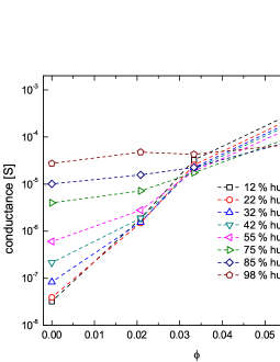
Figure 8: (Color online) Conductance versus $\phi$ dependence for a carbon black-quaternized Poly(4-vinylpyridine) composite for different humidities. Adapted from Ref. [Li2007b, ]

Let us now turn to discuss some consequences of the theory presented here. As shown in Sec. V the cross-over volume fraction $\phi_{c}$ depends explicitly on the conductivity $\sigma_{\rm m}$ of the insulating medium, leading to the possibility of shifting $\phi_{c}$ by altering $\sigma_{\rm m}$. Formulas (13) and (14) were obtained by assuming that the transport mechanism leading to $\sigma_{\rm m}$ was independent of the concentration of the conducting fillers, as it is the case for polymer-based nanocomposites, where the conduction within the polymer is due to ion mobility. In that case, a change in $\sigma_{\rm m}$, and so a change in $\phi_{c}$, could be induced by a change in the ion concentration. This is nicely illustrated by an example where a conductive polymer composite with large ionic conductivity was studied as a material for humidity sensors.Li2007b This consisted of carbon black dispersed in a Poly(4-vinylpyridine) matrix which was quaternized in order to obtain a polyelectrolyte. Since the absorbed water molecules interact with the polyelectrolyte and facilitate the ionic dissociation, higher humidity implies a larger ionic conductivity. In Fig. 8 we have redrawn Fig. 4 of Ref. [Li2007b, ] in terms of the conductance as a function of carbon black content for different humidity levels. Consistently with our assumptions, one can see that with the increase of humidity the matrix intrinsic conductivity is indeed shifted upward, while this has a weaker effect on the conductivity for higher contents of carbon black, where transport is governed by interparticle tunneling (a slight downshift in this region is attributed to enhanced interparticle distances due to water absorption). The net effect illustrated in Fig. 8 is thus a shift of the crossover point $\phi_{c}$ towards higher values of carbon black content. It is worth noticing that the explanation proposed by the authors of Ref. [Li2007b, ] in order to account for their finding is equivalent to the global tunneling network/crossover scenario.

Another feature which should be expected by the global tunneling network model concerns the response of the conductivity to an applied strain $\varepsilon$. Indeed, by using Eq. (3), the piezoresistive response $\Gamma$, that is the relative change of the resistivity $\sigma^{-1}$ upon an applied $\varepsilon$, reduces to:

$$\Gamma\equiv\frac{d\ln(\sigma^{-1})}{d\varepsilon}=\ln\!\left(\frac{\sigma_{0}}{\sigma}\right)\frac{d\ln(\delta_{c})}{d\varepsilon}.$$ (16)

In the above expression $d\ln(\delta_{c})/d\varepsilon=1$ for fillers having the same elastic properties of the insulating matrix. In contrast, for elastically rigid fillers this term can be rewritten as $[d\ln(\delta_{c})/d\ln(\phi)]d\ln(\phi)/d\varepsilon$, which is also approximatively a constant due to the $\delta_{c}$ dependence on $\phi$ as given in Eqs. (4), (8), and (9), and to $d\ln(\phi)/d\varepsilon\simeq-1$. Hence, the expected dominant dependence of $\Gamma$ is of the form $\Gamma\propto\ln(1/\sigma)$, which has been observed indeed in Refs.[Tamborin1997, ; Niki2009, ].

Finally, before concluding, we would like to point out that, with the theory presented in this paper, both the low temperature and the filler dependencies of nanocomposites in the dielectric regime have a unified theoretical framework. Indeed, by taking into account particle excitation energies, Eq. (2) can be generalized to include inter-particle electronic interactions, leading, within the critical path approximation, to a critical distance $\delta_{c}$ which depends also on such interactions and on the temperature. The resulting generalized theory would be equivalent then to the hopping transport theory corrected by the excluded volume effects of the impenetrable cores of the conducting particles. An example of this generalization for the case of nanotube composites is the work of Ref. [Hu2006, ].

In summary, we have considered the tunneling-percolation problem in the so far unstudied intermediate regime between the percolation-like and the hopping-like regimes by extending the critical path analysis to systems and properties that are pertinent to nanocomposites. We have analyzed published conductivity data for several nanotubes, nanofibers, nanosheets, and nanospheres composites and extracted the corresponding values of the tunneling decay length $\xi$. Remarkably, most of the extracted $\xi$ values fall within its expected range, showing that tunneling is a manifested characteristic of the conductivity of nanocomposites. Our formalism can be used to tailor the electrical properties of real composites, and can be generalized to include different filler shapes, filler size and/or aspect-ratio polydispersity, and interactions with the insulating matrix.

Appendix A Excluded volumes of spheroids and spherocylinders with isotropic orientation distribution

The work of Isihara Isihara1950 enables to derive closed relations for the excluded volume of two spheroids with a shell of constant thickness and for an isotropic distribution of the mutual orientation of the spheroid symmetry axes. Given two spheroids with polar semi-axis $a$ and equatorial semi-axis $b$, their eccentricity $\epsilon$ are defined as follows:

$$\epsilon= \sqrt{1-\frac{b^{2}}{a^{2}}}\qquad\qquad\textrm{for prolates},$$ (17)

$$\epsilon= \sqrt{1-\frac{a^{2}}{b^{2}}}\qquad\qquad\textrm{for oblates}.$$ (18)

If the mutual orientation of the spheroid symmetry axes is isotropic, the averaged excluded volume of the two spheroids is then (valid also for more general identical ovaloids)

$$V_{\rm exc}=2V+\frac{MF}{2\pi},$$ (19)

where $V$ is the spheroid volume and $M$ and $F$ are two quantities defined as:Isihara1950

$$M= 2\pi a\bigg{[}1+\frac{(1-\epsilon^{2})}{2\epsilon}\ln{\bigg{(}\frac{1+\epsilon}{1-\epsilon}\bigg{)}}\bigg{]},$$ (20)

$$F= 2\pi ab\bigg{(}\sqrt{1-\epsilon^{2}}+\frac{\arcsin{\epsilon}}{\epsilon}\bigg{)},$$ (21)

for the case of prolate ($a/b>1$) spheroids and

$$M= 2\pi b\bigg{(}\sqrt{1-\epsilon^{2}}+\frac{\arcsin{\epsilon}}{\epsilon}\bigg{)},$$ (22)

$$F= 2\pi b^{2}\bigg{[}1+\frac{(1-\epsilon^{2})}{2\epsilon}\ln{\bigg{(}\frac{1+\epsilon}{1-\epsilon}\bigg{)}}\bigg{]},$$ (23)

for the case of oblate ($a/b<1$) spheroids.

If now the spheroids are coated with a shell of uniform thickness $d$ ($d=\delta/2$), then the averaged excluded volume of the spheroids plus shell has again the form of (19):

$$V_{\rm exc}^{\rm tot}=2V_{d}+\frac{M_{d}F_{d}}{2\pi},$$ (24)

and by constructing the quantities $V_{d}$, $M_{d}$, and $F_{d}$ from their definition in Ref. [Isihara1950, ] (see Ref. [Ambrosetti2008, ] for a similar calculation), one obtains:

$$V_{\rm exc}^{\rm tot}=V_{\rm exc}+4dF+\frac{dM^{2}}{\pi}+8d^{2}M+\frac{32\pi}{3}d^{3}.$$ (25)

In the cases of extreme prolate ($a/b\gg 1$ and $\delta/a\ll 1$) and oblate ($a/b\ll 1$ and $\delta/b\ll 1$) spheroids, the total excluded volume reduces therefore to

$$V_{\rm exc}^{\rm tot}=V_{\rm exc}+2\pi a^{2}\delta,$$ (26)

for prolates and

$$V_{\rm exc}^{\rm tot}=V_{\rm exc}+4\pi b^{2}\delta+\pi^{3}b^{2}\delta/2+2\pi^{2}b\delta^{2},$$ (27)

for oblates. Within the second-order virial approximation, the critical distance $\delta_{c}$ is related to the volume fraction $\phi$ through $\phi\simeq V/\Delta V_{\rm exc}$, where $\Delta V_{\rm exc}=V_{\rm exc}^{\rm tot}-V_{\rm exc}$. From the above expressions one has then [$D=2\max(a,b)$]:

$$\phi\simeq\frac{(b/a)^{2}}{3\delta_{c}/D},$$ (28)

for prolates and

$$\phi\simeq\frac{(4/3)(a/b)}{(8+\pi^{2})\delta_{c}/D+8\pi(\delta_{c}/D)^{2}},$$ (29)

for oblates.

For comparison, we provide below the excluded volumes of randomly oriented spherocylinders. These are formed by cylinders of radius $R$ and length $L$, capped by hemispheres of radius $R$. Their volume is $V=(4/3)\pi R^{3}[1+(3/4)(L/R)]$. The excluded volume for spherocylinders with isotropic orientation distribution was calculated in Ref. [Balberg1984, ] and reads

$$V_{\rm exc}=\frac{32\pi}{3}R^{3}\left[1+\frac{3}{4}(L/R)+\frac{3}{32}(L/R)^{2}\right].$$ (30)

The excluded volume $V_{\rm exc}^{\rm tot}$ of spherocylinders with a shell of constant thickness $d=\delta/2$ is hen:

$$V_{\rm exc}^{\rm tot}=\frac{32\pi}{3}(R+d)^{3}\left[1+\frac{3}{4}\left(\frac{L}{R+d}\right)+\frac{3}{32}\left(\frac{L}{R+d}\right)^{2}\right].$$ (31)

For the high aspect-ratio limit ($L/R\gg 1$), when $d/L\ll 1$, the total excluded volume minus the excluded volume of the impenetrable core is

$$\Delta V_{\rm exc}=\pi L^{2}d,$$ (32)

which coincides with the last term of Eq. (26) if $d=\delta/2$ and $a=R+L/2\simeq L/2$. Furthermore, the second-order virial approximation ($\phi\simeq V/\Delta V_{\rm exc}$) gives:

$$\phi\simeq\frac{(b/a)^{2}}{2\delta_{c}/D},$$ (33)

which has a numerical coefficient different from Eq. (28) because for spherocylinders $V\simeq 2\pi ab^{2}$ (for $a/b\gg 1$) while for spheroids $V=4\pi ab^{2}/3$.

Appendix B Supplementary material. Conductivity versus critical distance plots

We show in the following Figs. 9-17 the complete set of plots of the natural logarithm of the sample conductivity $\sigma$ as a function of the geometrical percolation critical distance $\delta_{c}$ for different polymer nanocomposites, as used to obtain the $\xi$ values of Fig. 7 of the main article. In collecting the published results of $\sigma$ versus $\phi$, we have considered only those works where $a/b$ and $D=2\max(a,b)$ were explicitly reported. In the cases of documented variations of these quantities, we used their arithmetic mean. The $\phi$ dependence of the original published data was then converted into a $\delta_{c}$ dependence as follows. For fibrous systems (nanofibers, nanotubes), the filler shape was assimilated to spherocylinders, while for nanosheet systems it was assimilated to oblate spheroids. For prolate fillers $\delta_{c}$ was obtained from Eq. (5), for oblate fillers the values for $\delta_{c}$ were obtained from Eq. (8), while for spherical fillers, the values of $\delta_{c}$ were obtained from Eq. (9).

Since the model introduced in the main text is expected to be representative only if $\phi$ is sufficiently above $\phi_{c}$ to consider the effect of the insulating matrix negligible, for a given experimental curve, higher $\phi$ data were privileged, and lower density points sometimes omitted when deviating consistently from the main trend. The converted data were fitted to Eq. (15) of the main text and the results of the fit are reported in Figs. 9-17 by solid lines. The results for $2/\xi$ and $\ln(\sigma_{0})$ are also reported in the figures. As it may be appreciated from Figs. 9-17, in many instances the experimental data follow nicely a straight line, as predicted by Eq. (15) of the main text, while in others the data are rather scattered or deviate from linearity. In these latter cases, the fit to Eq. (15) is meant to capture the main linear trend of $\ln(\sigma)$ as a function of $\delta_{c}$. It should also be noticed that, in spite of the rather narrow distribution of the extracted $\xi$ values reported in Fig. 7 of the main text, the values of the prefactor $\sigma_{0}$ obtained from the fits are widely dispersed. This is of course due to the fact that, besides intrinsic variations of the tunneling prefactor conductance for different composites, interpolating the data to $\delta_{c}=0$ leads to a large variance of $\sigma_{0}$ even for minute changes of the slope. We did not notice any significant correlation between the extracted $\xi$ and $\sigma_{0}$ values.

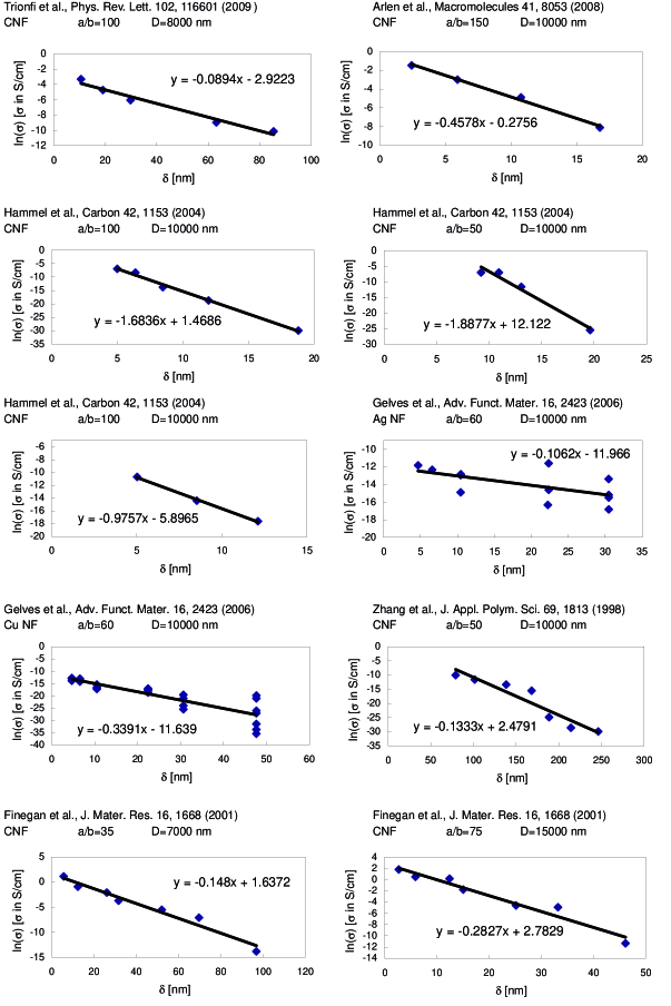
Figure 9: plots of $\ln\sigma$ as a function of $\delta$ for different polymer-nanofiber composites.

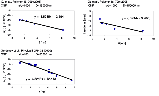
Figure 10: plots of $\ln\sigma$ as a function of $\delta$ for different polymer-nanofiber composites (cont.)

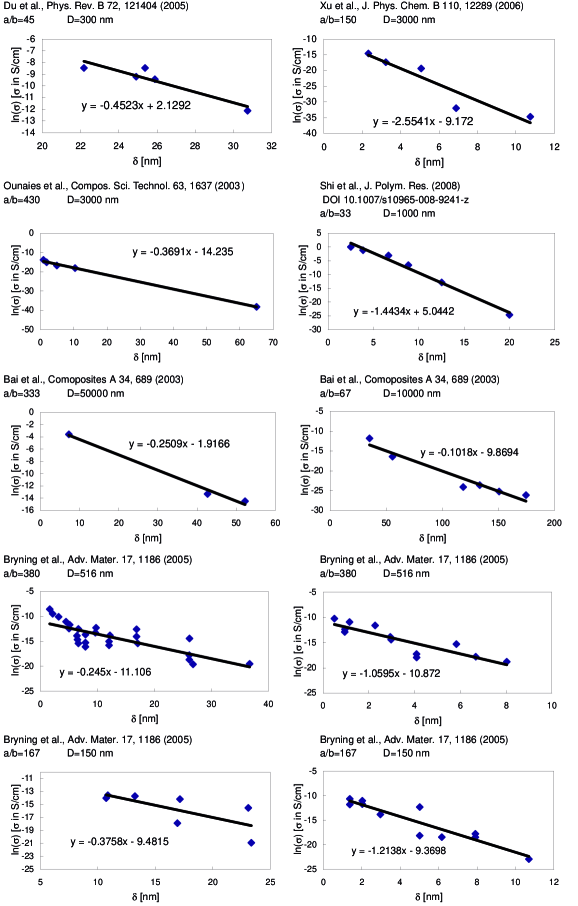
Figure 11: plots of $\ln\sigma$ as a function of $\delta$ for different polymer-nanotube composites.

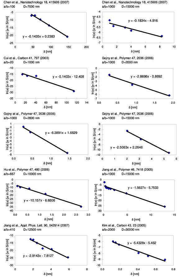
Figure 12: plots of $\ln\sigma$ as a function of $\delta$ for different polymer-nanotube composites (cont.)

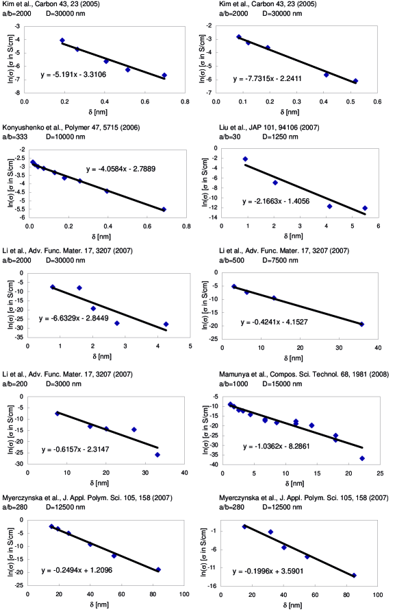
Figure 13: plots of $\ln\sigma$ as a function of $\delta$ for different polymer-nanotube composites (cont.)

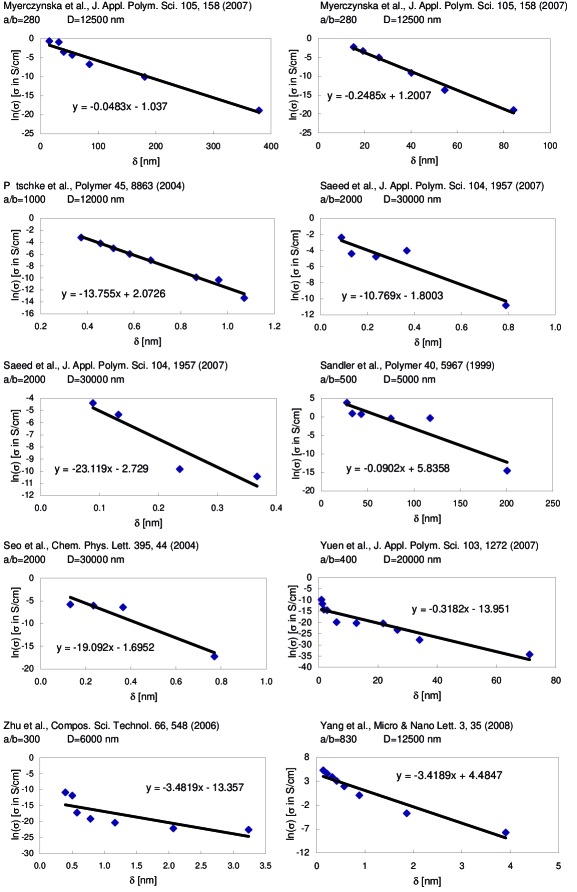
Figure 14: plots of $\ln\sigma$ as a function of $\delta$ for different polymer-nanotube composites (cont.)

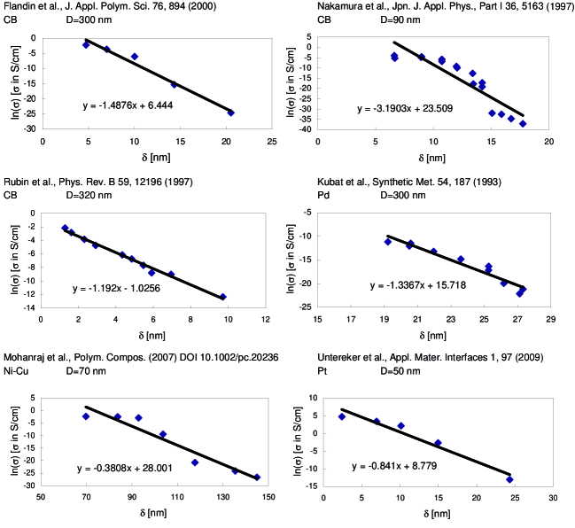
Figure 15: plots of $\ln\sigma$ as a function of $\delta$ for different polymer-nanospheres composites

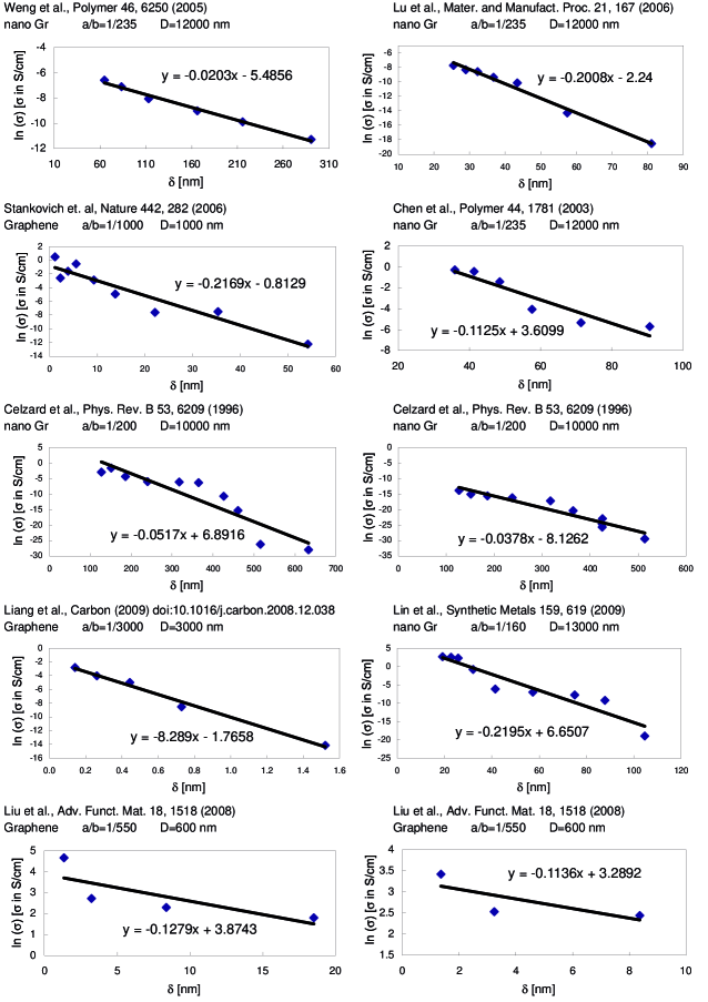
Figure 16: plots of $\ln\sigma$ as a function of $\delta$ for different polymer-nanosheet composites

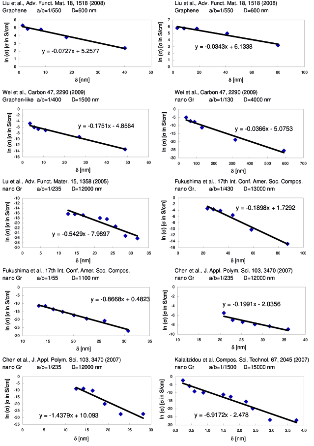
Figure 17: plots of $\ln\sigma$ as a function of $\delta$ for different polymer-nanosheet composites (cont.)

References

- (1) W. Bauhofer and J. Z. Kovacs, Compos. Sci. Technol. 69, 1486 (2009).
- (2) M. H. Al-Saleh and U. Sundararaj, Carbon 47, 2 (2009).
- (3) G. Eda and M. Chhowalla, Nano Lett. 9, 814 (2009).
- (4) S. Stankovich, D. A. Dikin, G. H. B. Dommett, K. M. Kohlhaas, E. J. Zimney, E. A. Stach, R. D. Piner, S. T. Nguyen, and R. S. Ruoff, Nature 442, 282 (2006).
- (5) T. Sekitani, H. Nakajima, H. Maeda, T. Fukushima, T. Aida, K. Hata, and T. Someya, Nature Mater. 8, 494 (2009).
- (6) S. Kirkpatrick, Rev. Mod. Phys. 45, 574 (1973)
- (7) D. Stauffer and A. Aharony, Introduction to Percolation Theory (Taylor & Francis, London 1994).
- (8) M. Sahimi, Heterogeneous Materials I. Linear Transport and Optical Properties (Springer, New York, 2003).
- (9) S. Vionnet-Menot, C. Grimaldi, T. Maeder, S. Strässler, and P. Ryser, Phys. Rev. B 71, 064201 (2005).
- (10) P. Sheng, E. K. Sichel, and J. I. Gittleman, Phys. Rev. Lett. 40, 1197 (1978).
- (11) I. Balberg, Phys. Rev. Lett. 59, 1305 (1987).
- (12) S. Paschen, M. N. Bussac, L. Zuppiroli, E. Minder, and B. Hilti, J. Appl. Phys. 78, 3230 (1995).
- (13) C. Li, E. T. Thorstenson, T.-W. Chou, Appl. Phys. Lett. 91, 223114 (2007).
- (14) I. Balberg, J. Phys. D: Appl. Phys. 42, 064003 (2009).
- (15) N. Johner, C. Grimaldi, I. Balberg and P. Ryser, Phys. Rev. B 77, 174204 (2008).
- (16) B. I. Shklovskii and A. L. Efros, Electronic Properties of Doped Semiconductors (Springer, Berlin, 1984).
- (17) V. Ambegaokar, B. I. Halperin, and J. S. Langer, Phys. Rev. B 4, 2612 (1971); M. Pollak, J. Non Cryst. Solids 11, 1 (1972): B. I. Shklovskii and A. L. Efros, Sov. Phys. JETP 33, 468 (1971); 34, 435 (1972).
- (18) C. H. Seager and G. E. Pike, Phys. Rev. B 10, 1435 (1974).
- (19) H. Overhof and P. Thomas, Hydrogetaned Amorphous Semiconductors (Springer, Berlin, 1989).
- (20) G. Ambrosetti, N. Johner, C. Grimaldi, T. Maeder, P. Ryser, and A. Danani, J. Appl. Phys. 106, 016103 (2009).
- (21) G. Ambrosetti, N. Johner, C. Grimaldi, A. Danani, and P. Ryser, Phys. Rev. E 78, 061126 (2008).
- (22) J. D. Sherwood, J. Phys. A: Math. Gen. 30, L839 (1997).
- (23) M. A. Miller, J. Chem. Phys. 131, 066101 (2009).
- (24) S. Torquato, Random Heterogeneous Materials: Microstructure and Macroscopic Properties (Springer, New York, 2002).
- (25) D. Frenkel and B. M. Mulder, Mol. Phys. 55 1171 (1985).
- (26) C. A. Miller and S. Torquato, J. Appl. Phys. 68, 5486 (1990).
- (27) T. Schilling, S. Jungblut, and M. A. Miller, Phys. Rev. Lett. 98, 108303 (2007).
- (28) P. Sheng and J. Klafter, Phys. Rev. B 27, 2583 (1983).
- (29) T. Hu and B. I. Shklovskii, Phys. Rev. B 74, 054205 (2006); Phys. Rev. B 74, 174201 (2006).
- (30) R. Fogelholm, J. Phys. C 13, L571 (1980).
- (31) Y. M. Strelniker, S. Havlin, R. Berkovits, and A. Frydman, Phys. Rev. E 72, 016121 (2005).
- (32) T. Blyte and D. Bloor, Electrical Properties of Polymers. (Cambridge University Press, Cambridge, 2005).
- (33) For the case in which there exist some electronic contribution to the matrix conductivity, the total conducivity is only approximately the sum of and . In this case a more precise esimate of could be obtained for example from an effective medium approximation.
- (34) T. Ota, M. Fukushima, Y. Ishigure, H. Unuma, M. Takahashi, Y. Hikichi, and H. Suzuki, J. Mater. Sci. Lett. 16, 1182 (1997).
- (35) K. Nagata, H. Iwabuki, and H. Nigo, Compos. Interfaces 6 483 (1999).
- (36) W. Lu, J. Weng, D. Wu, C. Wu, and G. Chen, Mater. Manuf. Process. 21, 167 (2006).
- (37) D. M. Heyes, M. Cass and A. C. Brańca, Mol. Phys. 104, 3137 (2006).
- (38) L. Berhan and A. M. Sastry, Phys. Rev. E 75, 041120 (2007).
- (39) A. V. Kyrylyuk and P. van der Schoot, Proc. Natl. Acad. Sci. USA 105, 8221 (2008).
- (40) I. Balberg, C. H. Anderson, S. Alexander, and N. Wagner, Phys. Rev. B 30, 3933 (1984)
- (41) A. L. R. Bug, S. A. Safran, and I. Webman, Phys. Rev. B 33, 4716 (1986).
- (42) The slight difference between these values of and those obtained from the numerical results could be attributed to finite-size effects, as proposed in Ref. [Kyrylyuk2008, ], or by the fact that the second-virial approximation is quantitatively correct only in the asymptotic regime.
- (43) M. P. Allen and M. R. Wilson, J. Comput. Aid. Mol. Des. 3, 335 (1989).
- (44) R. Eppenga and D. Frenkel, Mol. Phys. 52, 1303 (1984).
- (45) S. B. Kharchenko, J. F. Douglas, J. Obrzut, E. A. Grulke, and K. B Migler, Nature Mater. 3, 564 (2004).
- (46) I. Balberg, Phys. Rev. B 31, 4053 (1985).
- (47) J. Kubát, et al., Synthetic Met. 54, 187 (1993).
- (48) G. A. Gelves, B. Lin, U. Sundararaj, and J. A. Haber, Adv. Funct. Mater. 16, 2423 (2006).
- (49) M. B. Bryning, M. F. Islam, J. M. Kikkawa, and A. G. Yodh, Adv. Mater. 17, 1186 (2005).
- (50) A. Trionfi, D. H. Wang, J. D. Jacobs, L.-S. Tan, R. A. Vaia, and J.W. P. Hsu, Phys. Rev. Lett. 102, 116601 (2009); M. J. Arlen, D. Wang, J. D. Jacobs, R. Justice, A. Trionfi, J. W. P. Hsu, D. Schaffer, L.-S. Tan, and R. A. Vaia, Macromolecules 41, 8053 (2008); E. Hammel, X. Tang, M. Trampert, T. Schmitt, K. Mauthner, A. Eder, and P. Pötschke, Carbon 42 1153 (2004); C. Zhang, X.-S. Yi, H. Yui, S. Asai, and M. Sumita, J. Appl. Polym. Sci. 69, 1813 (1998); I. C. Finegan and G. G. Tibbetts, J. Mater. Res. 16, 1668 (2001); Y. Xu, B. Higgins, and W. J. Brittain, Polymer 46, 799 (2005); S. A. Gordeyev, F. J. Macedo, J. A. Ferreira, F. W. J. van Hattum, and C. A. Bernardo, Physica B 279, 33 (2000); F. Du, J. E. Fischer, and K. I. Winey, Phys. Rev. B 72, 121404(R) (2005) J. Xu, W. Florkowski, R. Gerhardt, K.-S. Moon, and C.-P. Wong, J. Phys. Chem. B 110, 12289 (2006); Z. Ounaies, C. Park, K. E. Wise, E. J. Siochi, and J. S. Harrison, Compos. Sci. Technol. 63, 1637 (2003); S.-L. Shi, L.-Z. Zhang, and J.-S. Li, J. Polym. Res. 16, 395 (2009); J. B. Bai, and A. Allaoui, Composites A 34, 689 (2003); H. Chen, H. Muthuraman, P. Stokes, J. Zou, X. Liu, J. Wang, Q. Huo, S. I. Khondaker, and L. Zhai, Nanotechnology 18 415606 (2007); S. Cui, R. Canet, A. Derre, M. Couzi, and P. Delhaes, Carbon 41, 797 (2003); F. H. Gojny, M. H. G. Wichmann, B. Fiedler, I. A. Kinloch, W. Bauhofer, A. H. Windle, and K. Schulte, Polymer 47, 2036 (2006); G. Hu, C. Zhao, S. Zhang, M. Yang, and Z. Wang, Polymer 47, 480 (2006); X. Jiang, Y. Bin, and M. Matsuo, Polymer 46, 7418 (2005); M.-J. Jiang, Z.-M. Dang, and H.-P. Xu, Appl. Phys. Lett. 90, 042914 (2007); Y. J. Kim , T. S. Shin, H. D. Choi, J. H. Kwon, Y.-C. Chung, H. G. Yoon, Carbon 43, 23 (2005); E. N. Konyushenko, J. Stejskal, M. Trchová, J. Hradil, J. Kovářová, J. Prokeš, M. Cieslar, J.-Y. Hwang, K.-H. Chen, and I. Sapurina, Polymer 47, 5715 (2006); L. Liu, S. Matitsine, Y. B. Gan, L. F. Chen, L. B. Kong, and K. N. Rozanov, J. Appl. Phys. 101, 094106 (2007); J. Li, P. C. Ma, W. S. Chow, C. K. To, B. Z. Tang, and J.-K. Kim, Adv. Funct. Mater. 17, 3207 (2007); Ye. Mamunya, A. Boudenne, N. Lebovka, L. Ibos, Y. Candau, and M. Lisunova, Compos. Sci. Technol. 68, 1981 (2008); A. Mierczynska, M. Mayne-L’Hermite, G. Boiteux, and J. K. Jeszka, J. Appl. Polym. Sci. 105, 158 (2007); P. Pötschke, M. Abdel-Goad, I. Alig, S. Dudkin, and D. Lellinger, Polymer 45, 8863 (2004); K. Saeed and S.-Y. Park, J. Appl. Polym. Sci. 104, 1957 (2007); J. Sandler, M. S. P. Shaffer, T. Prasse, W. Bauhofer, K. Schulte, and A. H. Windle, Polymer 40, 5967 (1999); M.-K. Seo, S.-J. Park, Chem. Phys. Lett. 395, 44 (2004); S.-M. Yuen, C.-C. M. Ma, H.-H. Wu, H.-C. Kuan, W.-J. Chen, S.-H. Liao, C.-W. Hsu, and H.-L. Wu, J. Appl. Polym. Sci. 103, 1272 (2007); B.-K. Zhu, S.-H. Xie, Z.-K. Xu, and Y.-Y. Xu, Compos. Sci. Technol. 66, 548 (2006); Y. Yang, M. C. Gupta, J. N. Zalameda, and W. P. Winfree, Micro Nano Lett. 3, 35 (2008).
- (51) L. Flandin, A. Chang, S. Nazarenko, A. Hiltner, and E. Baer, J. Appl. Polym. Sci. 76, 894 (2000); S. Nakamura, K. Saito, G. Sawa, and K. Kitagawa, Jpn. J. Appl. Phys. 36, 5163 (1997); Z. Rubin, S. A. Sunshine, M. B. Heaney, I. Bloom, and I. Balberg, Phys. Rev. B 59, 12196 (1999); G. T. Mohanraj, P. K. Dey, T. K. Chaki, A. Chakraborty, D. Khastgir, Polym. Compos. 28, 696 (2007); D. Untereker, S. Lyu, J. Schley, G. Martinez, and L. Lohstreter, ACS Appl. Mater. Interfaces 1, 97 (2009).
- (52) W. Weng, G. Chen, and D. Wu, Polymer 46, 6250 (2005); G. Chen, C. Wu, W. Weng, D. Wu, and W. Yan, Polymer 44, 1781 (2003); A. Celzard, E. McRae, C. Deleuze, M. Dufort, G. Furdin, and J. F. Marêché, Phys. Rev. B 53, 6209 (1996); J. Liang, Y. Wang, Y. Huang, Y. Ma, Z. Liu, J. Cai, C. Zhang, H. Gao, and Y. Chen, Carbon 47, 922 (2009); W. Lin, X. Xi, and C. Yu, Synthetic Met. 159, 619 (2009); N. Liu, F. Luo, H. Wu, Y. Liu, C. Zhang, and J. Chen, Adv. Funct. Mater. 18, 1518 (2008); T. Wei, G. L. Luo, Z. J. Fan, C. Zheng, J. Yan, C. Z. Yao, W. F. Li, and C. Zhang, Carbon 47, 2296 (2009); J. Lu, W. Weng, X. Chen, D. Wu, C. Wu, G. Chen, Adv. Funct. Mater. 15, 1358 (2005); H. Fukushima and L. T. Drzal, “Graphite nanoplatelets as reinforcements for polymers: structural and electrical properties”, 17th international conference of the American Society for Composites, Purdue University (2002); G. Chen, X. Chen, H. Wang, D. Wu, J. Appl. Polym. Sci. 103, 3470 (2007); K. Kalaitzidou, H. Fukushima, L. T. Drzal, Compos. Sci. Technol. 67, 2045 (2007).
- (53) R. E. Holmlin, R. Haag, M. L. Chabinyc, R. F. Ismagilov, A. E. Cohen, A. Terfort, M. A. Rampi, and G. M. Whitesides, J. Am. Chem. Soc. 123, 5075 (2001).
- (54) J. M. Benoit, B. Corraze, and O. Chauvet, Phys. Rev. B 65, 241405(R) (2002).
- (55) M. Ambrožič, A. Dakskobler, and M. Valent, Eur. Phys. J. Appl. Phys. 30, 23 (2005).
- (56) J. Hicks, A. Behnam, and A. Ural, Appl. Phys. Lett. 95, 213103 (2009)
- (57) Y. Li, L. Hong, Y. Chen, H. Wang, X. Lu, and M. Yang, Sens. Actuators B 123, 554 (2007).
- (58) M. Tamborin, S. Piccinini, M. Prudenziati, and B. Morten, Sens. Actuators A 58, 159 (1997).
- (59) Niklaus Johner, Ph. D thesis 4351, Ecole Polytechnique Fédérale de Lausanne (EPFL), (2009).
- (60) A. Isihara, J. Chem. Phys. 18, 1446 (1950)