Integral equation method for the electromagnetic wave propagation in stratified anisotropic dielectric-magnetic materials

Abstract

We investigate the propagation of electromagnetic waves in stratified anisotropic dielectric-magnetic materials using the integral equation method (IEM). Based on the superposition principle, we use Hertz vector formulations of radiated fields to study the interaction of wave with matter. We derive in a new way the dispersion relation, Snell’s law and reflection/transmission coefficients by self-consistent analyses. Moreover, we find two new forms of the generalized extinction theorem. Applying the IEM, we investigate the wave propagation through a slab and disclose the underlying physics which are further verified by numerical simulations. The results lead to a unified framework of the IEM for the propagation of wave incident either from a medium or vacuum in stratified dielectric-magnetic materials.

I Introduction

In electrodynamics, the integral equation method (IEM) is a powerful method for the electromagnetic wave propagation Born ; Jackson . From a microscopic perspective, a bulk material can be regarded as a collection of molecules (or atoms), each of which is a scatter and emits radiation under the action of an external field. The radiated retarded field and the exciting field interact to form the resultant transmitted field in the material. This formulation is often expressed as an integral equation and naturally leads to the well known Ewald-Oseen extinction theorem which is a basis of the scattering theory Born . The IEM relates the macroscopic electromagnetic responses of the material with the microscopic features of its constituent units, thus gives much deeper physical insight into the interaction of wave with material in contrast to the conventional approach of Maxwell theory Feynman1963 ; Wolf1972 . At the same time, the IEM does not require boundary conditions and is advantageous in some situations, especially when it is not sufficient to describe the interaction by the macroscopic Maxwell equations Wolf1972 ; Kong2001 ; Birman1972 ; Agarwal1973 . This approach has been widely used to study light scattering Kong2001 , the tip-sample interaction in near optics Girard1996 ; Novotny2006 and so on. By now, the interactions of waves with semi-infinite Reali1982 , a slab Reali1992 ; Lai2002 or stratified Karam1996 isotropic dielectric media have been treated by the IEM.

Recently, one kind of artificial anisotropic dielectric-magnetic materials, metamaterials, has attracted considerable attention simulated by its fascinating properties Veselago1968 ; Shelby2001 . To understand the unique characteristics of metamaterials it is necessary and appealing to take a microscopic viewpoint. On this issue, the IEM has been successfully implemented to predict the electric and magnetic resonances in split-ring resonators Zhou2008 , study the reflection of split-ring resonators Belov2006 and the imaging process of super lens Zhou2005 , and explain the Brewster phenomenon for TE wave associated with metamaterials Fu2005 ; Shu2007b . However, most previous work only consider the situation of semi-infinite materials and waves incident from vacuum. Then, how to treat the propagation of waves through stratified materials, especially for incidence from a material rather than vacuum? The latter problem is important because it will result in a completely new form of the extinction theorem, as shown in this paper.

The purpose of this paper is to use the IEM to investigate the properties of wave propagation in stratified anisotropic dielectric-magnetic media. Our emphasis is to disclose the underlying physics of electromagnetic interaction with matter rather that to obtain the well-known phenomenal results. On the basis of the superposition principle, we use Hertz vector formulations of radiated fields to study the microscopic mechanism of propagation. We arrive at new derivations of the dispersion relation, Snell’s law and reflection/transmission coefficients by self-consistent analyses. Moreover, we find two generalized forms of the extinction theorem. As an application, we use the IEM to study the wave propagation through a slab and discuss the physical process of photon tunneling, which are further verified through numerical simulations. The results lead to a unified framework of the IEM for the propagation of wave incident either from a medium or vacuum in stratified dielectric-magnetic materials.

II the integral formulation of Hertz vectors

In this section we take the microscopic viewpoint in which the matter consists of molecules that react to the exciting field like dipoles and formulate the radiated field in the form of a Green’s function integral of Hertz vectors.

Let a monochromatic electromagnetic field of ${\bf E}_{i}={\bf E}_{i0}\exp{(i{\bf k}_{i}\cdot{\bf r}-i\omega t)}$ and ${\bf H}_{i}={\bf H}_{i0}\exp{(i{\bf k}_{i}\cdot{\bf r}-i\omega t)}$ incident from an anisotropic material filling the semi-infinite space $z<0$. The $x-z$ plane is the plane of incidence and the schematic diagram is in Fig. 1. Since the material responds linearly, all the fields have the same dependence of $\exp{(-i\omega t)}$ which will be omitted subsequently for simplicity. Assume the reflected fields are ${\bf E}_{r}={\bf E}_{r0}\exp{(i{\bf k}_{r}\cdot{\bf r})}$ and ${\bf H}_{r}={\bf H}_{r0}\exp{(i{\bf k}_{r}\cdot{\bf r})}$, and the transmitted fields are ${\bf E}_{t}={\bf E}_{t0}\exp{(i{\bf k}_{t}\cdot{\bf r})}$ and ${\bf H}_{t}={\bf H}_{t0}\exp{(i{\bf k}_{t}\cdot{\bf r})}$. The permittivity and permeability tensors of the $n$-th layer are simultaneously diagonal in the principal coordinate system, $\bm{\varepsilon}_{n}=\hbox{diag}[\varepsilon_{nx},\varepsilon_{ny},\varepsilon_{nz}]$, $\bm{\mu}_{n}=\hbox{diag}[\mu_{nx},\mu_{ny},\mu_{nz}]$.

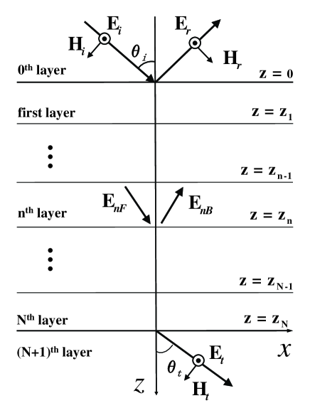
Figure 1: Schematic diagram for the reflection and refraction of TE waves in stratified media.

Inside the layers, the incident field drive the constituent unities to oscillate and radiate just as dipoles. The radiated electric fields by electric and magnetic dipoles are decided by Born ; Jackson ; Sein1989

$${\bf E}_{rad}=\nabla(\nabla\cdot{\bf{\Pi}}_{e})-\varepsilon_{0}\mu_{0}\frac{\partial^{2}{\bf{\Pi}}_{e}}{\partial t^{2}}-\mu_{0}\nabla\times\frac{\partial{\bf{\Pi}}_{m}}{\partial t}$$ (1)

and the magnetic fields generated by dipoles are

$${\bf H}_{rad}=\nabla(\nabla\cdot{\bf{\Pi}}_{m})-\varepsilon_{0}\mu_{0}\frac{\partial^{2}{\bf{\Pi}}_{m}}{\partial t^{2}}+\varepsilon_{0}\nabla\times\frac{\partial{\bf{\Pi}}_{e}}{\partial t}.$$ (2)

Here ${\bf\Pi}_{e}$ and ${\bf\Pi}_{m}$ are the Hertz vectors, which can be expressed as integrations of the Green’s function,

$${\bf\Pi}_{e}({\bf r})=\int_{V^{\prime}}\frac{{\bf P}({\bf r^{\prime}})}{\varepsilon_{0}}G({\bf r}-{\bf r}^{\prime})\hbox{d}{\bf r}^{\prime},$$ (3)

$${\bf\Pi}_{m}({\bf r})=\int_{V^{\prime}}{\bf M}({\bf r^{\prime}})G({\bf r}-{\bf r}^{\prime})\hbox{d}{\bf r}^{\prime}.$$ (4)

${\bf P}$ is the dipole moment density of electric dipoles and ${\bf M}$ is that of magnetic dipoles, which are related to the internal fields as ${\bf P}_{n}=\varepsilon_{0}\bm{\chi}_{en}\cdot{\bf E}_{n}$, ${\bf M}_{n}=\bm{\chi}_{mn}\cdot{\bf H}_{n}$, where the electric susceptibility $\bm{\chi}_{en}=(\bm{\varepsilon}_{n}/{\varepsilon_{0}})-1$ and the magnetic susceptibility $\bm{\chi}_{mn}=(\bm{\mu}_{n}/{\mu_{0}})-1$. Inside the layer, the dipoles produce forward waves as well as backward waves. So, we assume the dipole moment densities ${\bf P}$ and ${\bf M}$ have the following forms

$${\bf P}_{n}={\bf P}_{nF}\exp{(i{\bf k}_{nF}\cdot{\bf r})}+{\bf P}_{nB}\exp{(-i{\bf k}_{nB}\cdot{\bf r})},$$ (5)

$${\bf M}_{n}={\bf M}_{nF}\exp{(i{\bf k}_{nF}\cdot{\bf r})}+{\bf M}_{B}\exp{(-i{\bf k}_{nB}\cdot{\bf r})},$$ (6)

where ${\bf k}_{nF}$ stands for the forward wave and $-{\bf k}_{nB}$ stands for the backward wave Lai2002 ; Reali1992 . The wave numbers are to be decided by the dispersion relation yet to be derived. The Green function is $G({\bf r}-{\bf r}^{\prime})=\exp{(ik_{i}|{\bf r}-{\bf r}^{\prime}|)}/(4\pi|{\bf r}-{\bf r}^{\prime}|)$. To evaluate the Hertz vectors, we firstly represent the Green function in the Fourier form. Then, substituting it into Eqs. (3) and (4) and using the delta function definition and contour integration method Reali1982 ; Lai2002 , the Hertz vectors of the $n$-th layer can be evaluated as

$${\bf\Pi}_{en} = \frac{{\bf P}_{nF}}{\varepsilon_{0}}\{\frac{\exp{(i{\bf k}_{nF}\cdot{\bf r})}}{k_{nF}^{2}-q_{n}^{2}}+\frac{\exp{[i{\bf q}_{nF}\cdot{\bf r}+i(k_{nFz}-q_{nz})z_{n-1}]}}{2q_{nz}(q_{nz}-k_{nFz})}$$ (7)

$$\left.+\frac{\exp{[i{\bf q}_{nB}\cdot{\bf r}+i(k_{nFz}+q_{nz})z_{n}]}}{2q_{nz}(q_{nz}+k_{nFz})}\right\}+\frac{{\bf P}_{nB}}{\varepsilon_{0}}\left\{\frac{\exp{(-i{\bf k}_{nB}\cdot{\bf r})}}{k_{nB}^{2}-b_{n}^{2}}\right.$$

$$\left.+\frac{\exp{[-i{\bf b}_{nB}\cdot{\bf r}-i(k_{nBz}+b_{nz})z_{n-1}]}}{2b_{nz}(b_{nz}+k_{nBz})}+\frac{\exp{[-i{\bf b}_{nF}\cdot{\bf r}-i(k_{nBz}-q_{nz})z_{n}]}}{2b_{nz}(b_{nz}-k_{nBz})}\right\}$$

$$~{}~{}~{}~{}~{}~{}~{}~{}~{}~{}~{}~{}~{}~{}~{}~{}~{}~{}~{}~{}~{}~{}~{}~{}~{}~{}~{}~{}~{}~{}~{}~{}~{}~{}~{}~{}~{}~{}~{}~{}~{}~{}~{}~{}~{}~{}~{}~{}~{}~{}~{}~{}~{}~{}~{}~{}~{}~{}~{}~{}~{}~{}~{}~{}~{}~{}~{}~{}z_{n-1}\leq z\leq z_{n},$$

right to the material

$${\bf\Pi}_{en} = \frac{{\bf P}_{nF}}{\varepsilon_{0}}\frac{\exp{[i(k_{nFz}-q_{nz})z_{n-1}]}-\exp{[i(k_{nFz}-q_{nz})z_{n}]}}{2q_{nz}(q_{nz}-k_{nFz})}\exp{(i{\bf q}_{nF}\cdot{\bf r})}$$ (8)

$$+\frac{{\bf P}_{nB}}{\varepsilon_{0}}\frac{\exp{[-i(k_{nBz}+b_{nz})z_{n-1}]}-\exp{[-i(k_{nBz}+b_{nz})z_{n}]}}{2b_{nz}(b_{nz}+k_{nBz})}\exp{(-i{\bf b}_{nB}\cdot{\bf r})},$$

$$~{}~{}~{}~{}~{}~{}~{}~{}~{}~{}~{}~{}~{}~{}~{}~{}~{}~{}~{}~{}~{}~{}~{}~{}~{}~{}~{}~{}~{}~{}~{}~{}~{}~{}~{}~{}~{}~{}~{}~{}~{}~{}~{}~{}~{}~{}~{}~{}~{}~{}~{}~{}~{}~{}~{}~{}~{}~{}~{}~{}~{}~{}~{}~{}~{}~{}~{}~{}z>z_{n},$$

left to the material

$${\bf\Pi}_{en} = \frac{{\bf P}_{nF}}{\varepsilon_{0}}\frac{\exp{[i(k_{nFz}+q_{nz})z_{n}]}-\exp{[i(k_{nFz}+q_{nz})z_{n-1}]}}{2q_{nz}(q_{nz}+k_{nFz})}\exp{(i{\bf q}_{nB}\cdot{\bf r})}$$ (9)

$$+\frac{{\bf P}_{nB}}{\varepsilon_{0}}\frac{\exp{[-i(k_{nBz}-b_{nz})z_{n}]}-\exp{[-i(k_{nBz}-b_{nz})z_{n-1}]}}{2b_{nz}(b_{nz}-k_{nBz})}\exp{(-i{\bf b}_{nF}\cdot{\bf r})},$$

$$~{}~{}~{}~{}~{}~{}~{}~{}~{}~{}~{}~{}~{}~{}~{}~{}~{}~{}~{}~{}~{}~{}~{}~{}~{}~{}~{}~{}~{}~{}~{}~{}~{}~{}~{}~{}~{}~{}~{}~{}~{}~{}~{}~{}~{}~{}~{}~{}~{}~{}~{}~{}~{}~{}~{}~{}~{}~{}~{}~{}~{}~{}~{}~{}~{}~{}~{}~{}z<z_{n-1},$$

where we have used the following notations

$${\bf q}_{nF}=k_{nFx}\hat{{\bf x}}+q_{nz}\hat{{\bf z}},{\bf q}_{nB}=k_{nFx}\hat{{\bf x}}-q_{nz}\hat{{\bf z}},q_{nz}^{2}=k_{0}^{2}-k_{nFx}^{2};$$

$${\bf b}_{nF}=k_{nBx}\hat{{\bf x}}+b_{nz}\hat{{\bf z}},{\bf b}_{nB}=k_{nBx}\hat{{\bf x}}-b_{nz}\hat{{\bf z}},b_{nz}^{2}=k_{0}^{2}-k_{nBx}^{2}.$$ (10)

Note that the term with $\exp{(*)}$ equals zero if $(*)$ contains $z_{j}\rightarrow\pm\infty$, which can be found in the calculation. Then the Hertz vectors of arbitrary layers can be found in Eqs. (7)-(9). Analogous to ${\bf\Pi}_{ne}$, ${\bf\Pi}_{nm}$ can be obtained by interchanging ${\bf P}_{nF}/{\varepsilon_{0}}$ and ${\bf P}_{nB}/{\varepsilon_{0}}$ with ${\bf M}_{nF}$ and ${\bf M}_{nB}$, respectively. Inserting ${\bf\Pi}_{ne}$ and ${\bf\Pi}_{nm}$ into Eqs. (1) and (2), the radiated fields can be calculated out.

III Radiated Fields and Ewald-Oseen extinction theorem

In this section, we deduce the expressions of radiated fields generated by constituent unities in the propagation of waves in stratified anisotropic dielectric-magnetic media. Then we use the superposition principle to show how all the fields are combined to yield the reflected and transmitted fields inside the individual layers. By a self-consistent analysis we obtain the dispersion relation, Snell’s law and Fresnel’s coefficients. Moreover, we find two generalized forms of the extinction theorem.

III.1 Fields in the $n$-th layer

Inside the $n$-th layer, the layer by itself and the other layers all radiate under the action of external fields. Their radiated fields add up to the real fields inside this layer, that is,

$${\bf E}_{n}={\bf E}^{left.0}_{rad}+{\bf E}^{left}_{rad}+{\bf E}^{n}_{rad}+{\bf E}^{right}_{rad}+{\bf E}^{right.N+1}_{rad}.$$ (11)

Here the radiated field from the left semi-infinite space

$${\bf E}^{left.0}_{rad}=\left\{\begin{array}[]{ccc}\displaystyle\hfil&{\bf E}_{i0}\exp{(i{\bf k}_{i}\cdot{\bf r})},&\hbox{if}~{}z<0~{}\hbox{is vacuum;}\\ \displaystyle\hfil&-\frac{{\bf Q}({\bf q}_{0F},{\bm{P}}_{0F})}{2q_{0z}(q_{0z}-k_{0Fz})}-\frac{{\bf Q}(-{\bf b}_{0B},{\bm{P}}_{0B})}{2b_{0z}(b_{0z}+k_{0Bz})},&\hbox{or else},\end{array}\right.$$ (12)

the radiated field generated by the layer itself

$${\bf E}^{n}_{rad} = \frac{{\bf Q}({\bf k}_{nF},{\bm{P}}_{nF})}{k_{nFz}^{2}-q_{nz}^{2}}+\frac{\exp{[i(k_{nFz}-q_{nz})z_{n-1}]}}{2q_{nz}(q_{nz}-k_{nFz})}{\bf Q}({\bf q}_{nF},{\bm{P}}_{nF})$$ (13)

$$+\frac{\exp{[i(k_{nFz}+q_{nz})z_{n}]}}{2q_{nz}(q_{nz}+k_{nFz})}{\bf Q}({\bf q}_{nB},{\bm{P}}_{nF})+\frac{\exp{[-i(k_{nBz}+b_{n})z_{n-1}]}}{2b_{nz}(b_{nz}+k_{nBz})}{\bf Q}(-{\bf b}_{nB},{\bm{P}}_{nB})$$

$$+\frac{{\bf Q}({\bf k}_{nB},{\bm{P}}_{nB})}{k_{nBz}^{2}-b_{nz}^{2}}+\frac{\exp{[-i(k_{nBz}-b_{nz})z_{n}]}}{2b_{nz}(b_{nz}-k_{nBz})}{\bf Q}(-{\bm{b}}_{nF},{\bm{P}}_{nB}),$$

the radiated field generated by left layers $(1,\cdots,n-1)$

$${\bf E}^{left}_{rad} = \sum_{j=1}^{n-1}\frac{\exp{[i(k_{jFz}-q_{jz})z_{j-1}]}-\exp{[i(k_{jFz}-q_{jz})z_{j}]}}{2q_{jz}(q_{jz}-k_{jFz})}{\bf Q}({\bf q}_{jF},{\bm{P}}_{jF})$$ (14)

$$+\sum_{j=1}^{n-1}\frac{\exp{[-i(k_{jBz}+b_{jz})z_{j-1}]}-\exp{[-i(k_{jBz}+b_{jz})z_{j}]}}{2b_{jz}(k_{iz}+k_{jBz})}{\bf Q}(-{\bf b}_{jB},{\bm{P}}_{jB}),$$

the field radiated by right layers $(n+1,\cdots,N)$

$${\bf E}^{right}_{rad} = \sum_{j=n+1}^{N}\frac{\exp{[i(k_{jFz}+q_{jz})z_{j}]}-\exp{[i(k_{jFz}+q_{jz})z_{j-1}]}}{2q_{jz}(k_{jFz}+q_{jz})}{\bf Q}({\bf q}_{jB},{\bm{P}}_{jF})$$ (15)

$$+\sum_{j=n+1}^{N}\frac{\exp{[-i(k_{jBz}-b_{jz})z_{j}]}-\exp{[-i(k_{jBz}-b_{jz})z_{j-1}]}}{2b_{jz}(b_{jz}-k_{jBz})}{\bf Q}(-{\bf b}_{jF},{\bm{P}}_{jB}).$$

the radiated field from the right semi-infinite space

$${\bf E}^{right.N+1}_{rad}=\frac{-\exp{[i(k_{(N+1)Fz}+q_{(N+1)z})z_{N}]}}{2q_{(N+1)z}(k_{(N+1)Fz}+q_{(N+1)z})}{\bf Q}({\bf q}_{(N+1)B},{\bm{P}}_{(N+1)F}),$$ (16)

and ${\bf Q}$ is an auxiliary function

$${\bf Q}({\bf K},{\bm{P}})\equiv-\frac{1}{\varepsilon_{0}}\left[{\bf K}\times{\bf K}\times{\bm{P}}+({\bf K}^{2}-\varepsilon_{0}\mu_{0}\omega^{2}){\bm{P}}+\omega\mu_{0}\varepsilon_{0}{\bf K}\times{\bm{M}}\right]\exp{(i{\bf K}\cdot{\bf r})}$$ (17)

where ${\bf M}=\bm{\chi}_{m}\cdot[{\bf k}\times({\bf P}/\varepsilon_{0}\bm{\chi}_{e})/\bm{\mu}]/\omega$. There are two cases for the layer.

Case 1. The layer is an anisotropic dielectric-magnetic slab. Using ${\bf E}_{n}=[{\bf P}_{nF}\exp{(i{\bf k}_{F}\cdot{\bf r})}+{\bf P}_{nB}\exp{(-i{\bf k}_{B}\cdot{\bf r})}]/(\varepsilon_{0}\bm{\chi}_{ne})$ and inserting Eqs. (12) - (16) into Eq. (11), we come to the following conclusions.

(i). Checking terms associated with the incident field, we find that ${\bf q}_{1F}=-{\bf b}_{1B}={\bf q}_{0F}$, that is, $q_{1z}=b_{1z}$ and $k_{1Fx}=-k_{1Bx}=k_{ix}$ that is just the Snell’s law. The incident field is related to the radiated field as

$$-\frac{\exp{[i(k_{(n-1)Fz}-q_{(n-1)z})z_{n-1}]}}{2q_{(n-1)z}(q_{(n-1)z}-k_{(n-1)Fz})}{\bf Q}({\bf q}_{(n-1)F},{\bm{P}}_{(n-1)F})$$

$$-\frac{\exp{[-i(k_{(n-1)Bz}+q_{(n-1)z})z_{n-1}]}}{2q_{(n-1)z}(q_{(n-1)z}+k_{(n-1)Bz})}{\bf Q}({\bf q}_{(n-1)F},{\bm{P}}_{(n-1)B})$$

$$+\frac{\exp{[i(k_{nFz}-q_{nz})z_{n-1}]}}{2q_{nz}(q_{nz}-k_{nFz})}{\bf Q}({\bf q}_{nF},{\bm{P}}_{nF})+\frac{\exp{[-i(k_{nBz}+q_{nz})z_{n-1}]}}{2q_{nz}(q_{nz}+k_{nBz})}{\bf Q}({\bf q}_{nF},{\bm{P}}_{nB})=0,$$

$$~{}~{}~{}~{}~{}~{}~{}~{}~{}~{}~{}~{}~{}~{}~{}~{}~{}~{}~{}~{}~{}~{}~{}~{}~{}~{}~{}~{}~{}~{}~{}~{}~{}~{}~{}~{}~{}~{}~{}~{}~{}~{}~{}~{}~{}~{}~{}~{}~{}~{}~{}~{}~{}~{}~{}~{}~{}~{}~{}~{}~{}~{}~{}~{}~{}~{}~{}~{}~{}~{}~{}~{}~{}~{}~{}~{}~{}~{}~{}~{}n=1,\cdots,N.$$ (18)

This equation is actually the forward expression of the Ewald-Oseen extinction theorem. It shows quantitatively that the forward part of the radiation fields at a location in the layer extinguishes those from the regions left to that location.

(ii). Examining terms of the phase factors $\exp{(i{\bf q}_{n2}\cdot{\bf r})}$ and $\exp{(-i{\bf b}_{n1}\cdot{\bf r})}$ in Eq. (11), we know that ${\bf q}_{nB}=-{\bf b}_{nF}$. At the same time, we have

$$-\frac{\exp{[i(q_{(n+1)z}+k_{(n+1)Fz})z_{n})]}}{2q_{(n+1)z}(q_{(n+1)z}+k_{(n+1)Fz})}{\bf Q}({\bf q}_{(n+1)B},{\bm{P}}_{(n+1)F})$$

$$-\frac{\exp{[-i(k_{(n+1)Bz}-q_{(n+1)z})z_{n}]}}{2q_{(n+1)z}(q_{(n+1)z}-k_{(n+1)Bz})}{\bf Q}({\bf q}_{(n+1)B},{\bm{P}}_{(n+1)B})$$

$$+\frac{\exp{[i(q_{nz}+k_{nFz})z_{n}]}}{2q_{nz}(q_{nz}+k_{nFz})}{\bf Q}({\bf q}_{nB},{\bm{P}}_{nF})+\frac{\exp{[-i(k_{nBz}-q_{nz})z_{n}]}}{2q_{nz}(q_{nz}-k_{nBz})}{\bf Q}({\bf q}_{nB},{\bm{P}}_{nB})=0,$$

$$~{}~{}~{}~{}~{}~{}~{}~{}~{}~{}~{}~{}~{}~{}~{}~{}~{}~{}~{}~{}~{}~{}~{}~{}~{}~{}~{}~{}~{}~{}~{}~{}~{}~{}~{}~{}~{}~{}~{}~{}~{}~{}~{}~{}~{}~{}~{}~{}~{}~{}~{}~{}~{}~{}~{}~{}~{}~{}~{}~{}~{}~{}~{}~{}~{}~{}~{}~{}~{}~{}~{}~{}~{}~{}~{}~{}~{}~{}~{}~{}n=1,\cdots,N.$$ (19)

Eq. (III.1) is the backword form of the Ewald-Oseen extinction theorem. It indicates the extinction of the backward vacuum fields in the layer by those from right to the layer. Eqs. (III.1) and (III.1) are two new forms of the extinction theorem that generalize the previous results to the case of incidence from a material rather than vacuum Wolf1972 ; Karam1996 .

(iii). From terms with the phase factors $\exp{(i{\bf k}_{nF}\cdot{\bf r})}$ or $\exp{(-i{\bf k}_{nB}\cdot{\bf r})}$ in Eq. (11) follows the dispersion relation

$$\frac{k_{nx}^{2}}{\mu_{nz}\varepsilon_{ny}}+\frac{k_{nz}^{2}}{\mu_{nx}\varepsilon_{ny}}=\omega^{2}$$ (20)

for TE waves. So $k_{nFz}=k_{nBz}$. Eq. (20) relates all the propagation modes in different layers.

Case 2. The layer is vacuum. Assuming the field in the layer ${\bf E}_{n}={\bf E}_{nF}\exp{(i{\bf k}_{nF}\cdot{\bf r})}+{\bf E}_{nB}\exp{(-i{\bf k}_{nB}\cdot{\bf r})}$, we arrive at

$${\bf E}_{nF} = -\frac{\exp{[i(k_{(n-1)Fz}-q_{(n-1)z})z_{n-1}]}}{2q_{(n-1)z}(q_{(n-1)z}-k_{(n-1)Fz})}{\bf Q}({\bf q}_{(n-1)F},{\bm{P}}_{(n-1)F})$$ (21)

$$-\frac{\exp{[-i(k_{(n-1)Bz}+q_{(n-1)z})z_{n-1}]}}{2q_{(n-1)z}(q_{(n-1)z}+k_{(n-1)Bz})}{\bf Q}({\bf q}_{(n-1)F},{\bm{P}}_{(n-1)B}),$$

and

$${\bf E}_{nB} = -\frac{\exp{[i(q_{(n+1)z}+k_{(n+1)Fz})z_{n}]}}{2q_{(n+1)z}(q_{(n+1)z}+k_{(n+1)Fz})}{\bf Q}({\bf q}_{(n+1)B},{\bm{P}}_{(n+1)F})$$ (22)

$$-\frac{\exp{[-i(k_{(n+1)Bz}-q_{(n+1)z})z_{n}]}}{2q_{(n+1)z}(q_{(n+1)z}-k_{(n+1)Bz})}{\bf Q}({\bf q}_{(n+1)B},{\bm{P}}_{(n+1)B})$$

From Eqs. (21) and (22), it seems that the field in the layer was only related with the adjacent regions. However, it is only a mathematical impression because physically all the fields from the whole space contribute to the field in the layer, as shown in Eq. (11) obviously.

III.2 The Reflected Field

In region $z<0$, the contributions of radiations from all regions form the real fields, yielding

$${\bf E}_{i}+{\bf E}_{r}={\bf E}^{0}_{rad}+{\bf E}^{right}_{rad}+{\bf E}^{right.N+1}_{rad}.$$ (23)

The field radiated by the material in the region $z<0$ can be obtained like Eq. (13)

$${\bf E}^{0}_{rad}=\frac{{\bf Q}({\bf k}_{0F},{\bm{P}}_{0F})}{k_{0Fz}^{2}-q_{0z}^{2}}+\frac{{\bf Q}({\bf q}_{0B},{\bm{P}}_{0F})}{2q_{0z}(q_{0z}+k_{0Fz})}+\frac{{\bf Q}({\bf k}_{0B},{\bm{P}}_{0B})}{k_{0Bz}^{2}-b_{0z}^{2}}+\frac{{\bf Q}(-{\bm{b}}_{0F},{\bm{P}}_{0B})}{2b_{0z}(b_{0z}-k_{0Bz})}.$$ (24)

Then we have the extinction of backward vacuum waves

$$\frac{{\bf Q}({\bf q}_{0B},{\bm{P}}_{0F})}{2q_{0z}(q_{0z}+k_{0Fz})}+\frac{{\bf Q}({\bf q}_{0B},{\bm{P}}_{0B})}{2q_{0z}(q_{0z}-k_{0Bz})}-\frac{{\bf Q}({\bf q}_{1B},{\bm{P}}_{1F})}{2q_{1z}(q_{1z}+k_{1Fz})}-\frac{{\bf Q}({\bf q}_{1B},{\bm{P}}_{1B})}{2q_{1z}(q_{1z}-k_{1Bz})}=0.$$ (25)

The incident and reflected fields have the following forms

$${\bf E}_{i}=\frac{{\bf P}_{0F}}{\varepsilon_{0}\bm{\chi}_{0e}}\exp{(i{\bf k}_{0F}\cdot{\bf r})},~{}~{}~{}~{}{\bf E}_{r}=\frac{{\bf P}_{0B}}{\varepsilon_{0}\bm{\chi}_{0e}}\exp{(-i{\bf k}_{0B}\cdot{\bf r})},~{}~{}~{}~{}~{}~{}~{}~{}~{}~{}~{}z<0.$$ (26)

By solving the above equations one can obtain the dispersion relation like Eq. (20) and the reflected field. If the region $z<0$ is vacuum, then

$${\bf E}_{r}=\frac{{\bf Q}({\bf q}_{1B},{\bm{P}}_{1F})}{2q_{1z}(q_{1z}+k_{1Fz})}+\frac{{\bf Q}({\bf q}_{1B},{\bm{P}}_{1B})}{2q_{1z}(q_{1z}-k_{1Bz})},~{}~{}~{}~{}~{}~{}~{}~{}~{}~{}~{}~{}~{}~{}z<0.$$ (27)

Eq. (27) is well known in previous work in the case of incidence from vacuum Karam1996 ; Lai2002 . Differently, Eq. (25) is a completely new form of the backward extinction theorem because the region $z<0$ is not vacuum but a material in which the scatters are induced to generate radiated field. Using it one can treat the problem of electromagnetic interaction for the incidence from either vacuum or a material.

III.3 The Transmitted Field

In the region $z>z_{N}$, the radiated fields generated by all regions form the transmitted field. That is,

$${\bf E}_{t}={\bf E}^{left.0}_{rad}+{\bf E}^{left}_{rad}+{\bf E}^{N+1}_{rad},$$ (28)

where the radiated field produced by dipoles in the region $z>z_{N}$ is

$${\bf E}^{N+1}_{rad}=\frac{{\bf Q}({\bf q}_{(N+1)F},{\bm{P}}_{(N+1)F})}{k_{(N+1)Fz}^{2}-q_{(N+1)z}^{2}}+\frac{\exp{[i(k_{(N+1)Fz}-q_{(N+1)z})z_{N}]}}{2q_{(N+1)z}(q_{(N+1)z}-k_{(N+1)Fz})}{\bf Q}({\bf q}_{(N+1)F},{\bm{P}}_{(N+1)F}).$$ (29)

Hence, one can easily obtain

$$\frac{\exp{[i(k_{(N+1)Fz}-q_{(N+1)z})z_{N}]}}{2q_{(N+1)z}(q_{(N+1)z}-k_{(N+1)Fz})}{\bf Q}({\bf q}_{(N+1)F},{\bm{P}}_{(N+1)F})$$

$$-\frac{\exp{[i(q_{Nz}-k_{NFz})z_{N}]}}{2q_{Nz}(q_{Nz}-k_{NFz})}{\bf Q}({\bf q}_{NB},{\bm{P}}_{NF})-\frac{\exp{[-i(k_{NBz}+q_{Nz})z_{N}]}}{2q_{Nz}(q_{Nz}+k_{NBz})}{\bf Q}({\bf q}_{NB},{\bm{P}}_{NB})=0$$

which describes that the forward vacuum wave generated by the material in the right self-half space is extinguished by the counterpart from to the region $z\leq z_{N}$. The transmitted field is assumed to be

$${\bf E}_{t}=\frac{{\bf P}_{(N+1)F}}{\varepsilon_{0}\bm{\chi}_{(N+1)e}}\exp{(i{\bf k}_{(N+1)F}\cdot{\bf r})}$$ (31)

If the region $z>z_{N}$ is vacuum, then

$${\bf E}_{t}=-\frac{\exp{[i(k_{NFz}-q_{Nz})z_{N}]}}{2q_{Nz}(q_{Nz}-k_{NFz})}{\bf Q}({\bf q}_{NF},{\bm{P}}_{NF})-\frac{\exp{[-i(k_{NBz}+q_{Nz})z_{N}]}}{2q_{Nz}(q_{Nz}+k_{NBz})}{\bf Q}({\bf q}_{NF},{\bm{P}}_{NB}),$$

$$~{}~{}~{}~{}~{}~{}~{}~{}~{}~{}~{}~{}~{}~{}~{}~{}~{}~{}~{}~{}~{}~{}~{}~{}~{}~{}~{}~{}~{}~{}~{}~{}~{}~{}~{}~{}~{}~{}~{}~{}~{}~{}~{}~{}~{}~{}~{}~{}~{}~{}~{}~{}~{}~{}~{}~{}~{}~{}~{}~{}~{}~{}z>0.$$ (32)

By solving the equations one can obtain the transmitted field and the dispersion relation in the region.

III.4 Transformation Matrix

Actually, it is not difficult to obtain the reflected field and the transmitted field. Using Eqs. (III.1), (III.1), (25), and (III.3) (Eqs. (21), (22), (27), and (III.3) if the associated region is vacuum), one can derive the mutual relationship of ${\bf E}_{n}$ in all regions

$$\left(\begin{array}[]{c}{\bm{E}}_{nF}\\ {\bm{E}}_{nB}\end{array}\right)=L_{n(n+1)}\left(\begin{array}[]{c}{\bm{E}}_{(n+1)F}\\ {\bm{E}}_{(n+1)B}\end{array}\right),\,n=0,\cdots,(N+1).$$ (33)

The transformation matrix $L_{n(n+1)}$ for TE waves is

$$L_{n(n+1)}=\frac{1}{T_{n{(n+1)}}}\left(\begin{array}[]{cc}\exp{[i(k_{(n+1)Fz}-k_{nFz})z_{n}]}&R_{n{(n+1)}}\exp{[-i(k_{nFz}+k_{(n+1)Fz})z_{n}]}\\ R_{n{(n+1)}}\exp{[i(k_{nFz}+k_{(n+1)Fz})z_{n}]}&\exp{[i(k_{nFz}-k_{(n+1)Fz})z_{n}]}\end{array}\right),$$ (36)

where

$$R_{n{(n+1)}}=\frac{\mu_{(n+1)x}k_{nFz}-\mu_{nx}k_{(n+1)Fz}}{\mu_{(n+1)x}k_{nFz}+\mu_{nx}k_{(n+1)Fz}},\,T_{n{(n+1)}}=\frac{2\mu_{(n+1)x}k_{nFz}}{\mu_{(n+1)x}k_{nFz}+\mu_{nx}k_{(n+1)Fz}}.$$ (38)

Note that ${\bm{E}}_{(N+1)B}=0$. Then, with Eqs. (26), (31) and (33) we finally obtain the real reflected and transmitted fields in individual layers.

The magnetic fields can be obtained just as the corresponding electric fields after replacing the function ${\bf Q}({\bf K},{\bm{P}})$ with ${\bf O}({\bf K},{\bm{M}})$,

$${\bf O}({\bf K},{\bm{M}})\equiv-\left({\bf K}\times{\bf K}\times{\bm{M}}+{\bf K}^{2}{\bm{M}}-\varepsilon_{0}\mu_{0}\omega^{2}{\bm{M}}-\omega{\bf K}\times{\bm{P}}\right)\exp{(i{\bf K}\cdot{\bf r})},$$ (39)

where ${\bf P}=\varepsilon_{0}\bm{\chi}_{e}\cdot{\bf E}=-\varepsilon_{0}\bm{\chi}_{e}\cdot[{\bf k}\times({\bf M}/\bm{\chi}_{m})/\bm{\varepsilon}]/\omega$.

By now, we have derived in a new way the reflected/transmitted fields and the reflection/transmission coefficients in stratified media. Although involving some seemingly complicated integrals that nevertheless have simple solutions, the IEM leads almost miraculously to the correct results. Obviously, Eqs. (33) and (40) are in agreement with the results obtained by the formal approach of Maxwell theory Born .

It seems from Eqs. (III.1), (III.1), (25), or (III.3) as if the extinction only occurs on the interfaces Wolf1972 . In fact, however, the vacuum fields are extinct at every points in all regions, as shown evidently in Eqs. (11), (23) or (31). In the above analyses of this section we do not presume any boundary condition. Instead, one can find that the result of Eq. (33) plays the role of boundary conditions in Maxwell theory Kong2000 .

IV Propagation through a slab

As an application of the IEM, we discuss the case of a three-layer configuration. For the case of $N=1$, by Eqs. (26) and (31) we obtain the reflection coefficient $R_{TE}={E}_{r0}/{E}_{i0}$ and the transmission coefficient $T_{TE}={E}_{t0}/{E}_{i0}$ for TE waves

$$R_{TE}=\frac{R_{01}+R_{12}e^{i2k_{1Fz}z_{1}}}{1+R_{01}R_{12}e^{i2k_{1Fz}z_{1}}},~{}~{}~{}T_{TE}=\frac{T_{01}T_{12}e^{ik_{1Fz}z_{1}}}{1+R_{01}R_{12}e^{i2k_{1Fz}z_{1}}}.$$ (40)

To further demonstrate the validity of the IEM, we calculate the propagating fields in photon tunneling and compare the results by IEM with those by solving Maxwell equations plus boundary conditions Born ; Kong2000 .

Consider a plane wave incident through a slab sandwiched between two prisms at the angle larger than critical angle. We calculate the transmitted field in the second prism by the IEM and the Maxwell approach, denoted by $|{\bf E}_{t}|_{IEM}$ and $|{\bf E}_{t}|_{Maxwell}$ respectively, as shown in Fig. 2.

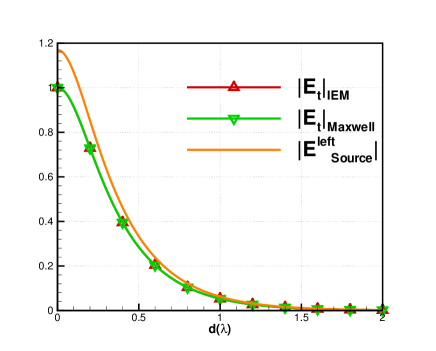
Figure 2: The field magnitude as a function of the width of the slab $d$. A TE-polarized plane wave is incident on the air gap sandwiched by two prisms with the dielectric constant $2.576$ at the angle $\pi/4$.

From that figure, we can see the two results overlap each other, indicating that the IEM is consistent with Maxwell approach and thus is valid. In order to disclose the physical mechanism of photon tunneling, we calculate the radiated fields $|{\bf E}^{left}_{Source}|$ from the left to the second prism, which is the source of the transmitted field. One can see that the amplitude of ${\bf E}^{left}_{Source}$ decreases exponentially as the width of the slab increases. Such a trend also occurs to $|{\bf E}_{t}|_{IEM}$. This phenomenon can be understood easily as the transmitted field results from the radiated field induced by ${\bf E}^{left}_{Source}$. Especially, we find that when $|{\bf E}^{left}_{Source}|$ approaches zero, the transmitted field is also close to zero. In other words, photon tunneling can not occur without the radiated field ${\bf E}^{left}_{Source}$ from the left region. Actually, detailed analyses show that the physical process of photon tunneling is that the vacuum field ${\bf E}^{left}_{Source}$ induce the dipoles in the second prism to radiate two kinds of waves; one of the radiated fields extinct ${\bf E}^{left}_{Source}$ and the other forms the final transmitted field, leading to photon tunneling. Based on the above results, we make numerical simulations of photon tunneling for slabs with different widths in Fig. 3. For completeness, we give results for both positive and negative indices.

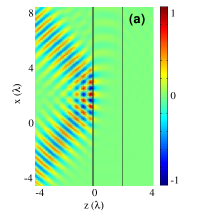
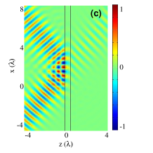
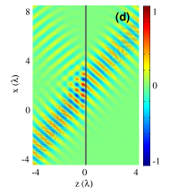
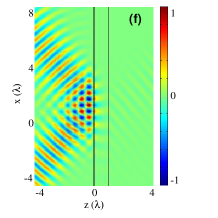
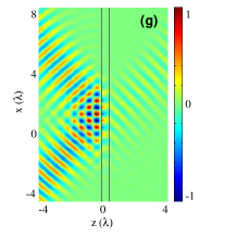
Figure 3: Field distributions for a Gaussian beam through slabs with different widths $d$. (a) $d=2\lambda$, (b) $d=\lambda$, (c) $d=0.5\lambda$, (d) $d=0.1\lambda$ for the slab with $\varepsilon_{1y}=1$ and $\mu_{1x}=\mu_{1z}=1$; (e) $d=2\lambda$, (f) $d=\lambda$, (g) $d=0.5\lambda$; (h) $d=0.1\lambda$ for the slab with $\varepsilon_{1y}=-1$ and $\mu_{1x}=\mu_{1z}=-1$. The slab is sandwiched by two prisms with the dielectric constant $2.576$ and the incident angle is $\pi/4$.

From Fig. 3, one can see that the photon tunneling mostly occurs as the slab is thinner than a wavelength and the transmitted field increases as the slab width decreases. At the same time, positive or negative Goos–Hänchen shifts are confirmed in photon tunneling as observed in Kong2002 .

V Conclusions

In summary, we have extended the IEM to investigate the propagation of electromagnetic waves through stratified anisotropic dielectric-magnetic media. From a microscopic viewpoint in which the matter consists of molecular scatters, we used the superposition principle and the integral formulation of Hertz vectors to analyze the interaction of field with matter. We presented new derivations of the dispersion relation, Snell’s law and the reflection/transmission coefficients by self-consistent analyses. Applying the IEM, we investigate the wave propagation through a slab and discuss the physical process of photon tunneling. Verified by numerical simulations, the results are in agreement with those obtained by macroscopic Maxwell theory and disclose the underlying physics of wave propagation through stratified materials, which is the emphasis of the present paper. Moreover, we found two new forms of the extinction theorem generalized to incidence not from vacuum but from a material, which may enrich the theory of molecular optics Born ; Wolf1972 ; Karam1996 . We also demonstrated that the extinction occurs at an arbitrary location inside the materials, not just on the interfaces Wolf1972 . Obviously, we recovered previous results for materials of positive refraction index Reali1992 ; Lai2002 ; Karam1996 . More importantly, our results lead to a unified framework of the IEM for wave propagation in stratified dielectric-magnetic materials.

The unified IEM can be applied to other problems of propagation through dielectric-magnetic materials, including metamaterials. This is because the units of metamaterials, whose dimensions are much less than the wavelength, react to exciting fields just as molecular scatters in conventional media Pendry2006 . Especially, the method can treat propagations of wave incident either from a medium or vacuum, in contrast with previous work Karam1996 ; Lai2002 in which only the incidence from vacuum is considered. Besides, the same framework not only enables the handling of arbitrary shaped objects made of continuous matter, but allows one to treat discrete particles. The associated coupling can be included in the IEM without any formal difficulty Girard1996 ; Novotny2006 . It is hoped that the framework and the microscopic perspective of the IEM may enable more unique properties in metamaterials to be understood and more applications to be developed.

References

• (1) M. Born and E. Wolf, Principles of Optics, Cambridge, Cambridge, (1999), p.110.
• (2) J. D. Jackson, Classical Electrodynamics, John Wiley & Sons, New York, (1999), p.280.
• (3) R. P. Feynman, R. B. Leighton, and M. Sands, The Feynman Lectures on Physics, Addison-Wesley, (1963).
• (4) E. Lalor and E. Wolf, J. Opt. Soc. Am. 62 (1972) 1165.
• (5) L. Tsang, J. A. Kong, and K. H. Ding, Scattering of Electromagnetic Waves: Theories and Applications, John Wiley & Sons Inc, New York, (2000).
• (6) J. L. Birman and J. J. Sein, Phys. Rev. B 6 (1972) 2482.
• (7) G. S. Agarwal, Phys. Rev. B 11 (1973) 1342.
• (8) C. Girard and A. Dereux, Rep. Prog. Phys. 59 (1996) 657.
• (9) L. Novotny and B. Hecht, Principles of Nano-Optics, Cambridge University Press, New York, (2006).
• (10) G. C. Reali, J. Opt. Soc. Am. 72 (1982) 1421.
• (11) G. C. Reali, Am. J. Phys. 60 (1992) 532.
• (12) H. M. Lai, Y. P. Lau, and W. H. Wong, Am. J. Phys. 70 (2002) 173.
• (13) M. A. Karam, J. Opt. Soc. Am. A 13 (1996) 2208.
• (14) V. G. Veselago, Sov. Phys. Usp. 10 (1968) 509.
• (15) R. A. Shelby, D. R. Smith, and S. Schultz, Science 292 (2001) 77.
• (16) X. Huang, Y. Zhang, C. T. Chan, and L. Zhou, Phys.Β Rev.Β B77 (2008) 235105.
• (17) P. A. Belov, Phys.Β Rev.Β B73 (2006) 045102.
• (18) L. Zhou, X. Huang, and C. T. Chan, Photonics and Nanostructures 3 (2005) 100.
• (19) C. Fu, Z. M. Zhang, and P. N. First, Applied Optics. 44 (2005) 3716.
• (20) W. X. Shu, Z. Ren, H. L. Luo, and F. Li, Euro. Phys. J. D 41 (2007) 541.
• (21) J. J. Sein, Am. J. Phys. 57 (1989) 837.
• (22) J. B. Pendry, Nature Materials 5 (2006) 599.
• (23) J. A. Kong, Electromagnetic Wave Theory, EMW Publishing, Cambridge, (2000), p.393.
• (24) J. A. Kong, B.-I. Wu, Y. Zhang, Appl.Β Phys.Β Lett.Β , 80 (2002) 2084.