Anomalous ordering in inhomogeneously strained materials

Abstract

We study a continuous quasi two-dimensional order-disorder phase transition that occurs in a simple model of a material that is inhomogeneously strained due to the presence of dislocation lines. Performing Monte Carlo simulations of different system sizes and using finite size scaling, we measure critical exponents describing the transition of $\beta=0.18\pm 0.02$, $\gamma=1.0\pm 0.1$, and $\alpha=0.10\pm 0.02$. Comparable exponents have been reported in a variety of physical systems. These systems undergo a range of different types of phase transitions, including structural transitions, exciton percolation, and magnetic ordering. In particular, similar exponents have been found to describe the development of magnetic order at the onset of the pseudogap transition in high-temperature superconductors. Their common universal critical exponents suggest that the essential physics of the transition in all of these physical systems is the same as in our simple model. We argue that the nature of the transition in our model is related to surface transitions although our model has no free surface.

Figure 1: (Color online) A) Magnetization order parameter $\langle|m|\rangle$ for the $x$-$y$ cross section, averaged over sites in the $z$ direction, of a $45\times 91\times 40$ system at a temperature of $4.49~{}k_{B}$. The order-enhanced and order-suppressed zones are shown in blue (dark) and yellow (light), respectively. B) Contour plot of the same data. The contour lines are in a step of $0.025$. The innermost line in the blue (dark) order-enhanced region corresponds to $0.55$.

Figure 2: (Color online) Finite size scaling data collapses for a quasi two-dimensional layer at the surface of an ordered cylindrical nucleus. The black circles correspond to an $x$-$y$ cross section circumference of 50, the red squares to a circumference of 102 and the green diamonds to a circumference of 200. The critical exponent $\nu=2.0$ and the critical temperature is $T_{c}=6.7$. A) Magnetization scaling function $\langle|\tilde{m}|\rangle$ vs. $|\tilde{t}|$ using the long range order critical exponent $\beta=0.18$. B) Susceptibility scaling function $\tilde{\chi}$ vs. scaled reduced temperature $\tilde{t}$ using the critical exponent $\gamma=1.0$. C) Specific heat scaling function $\tilde{c}$ vs. $\tilde{t}$ using the critical exponent $\alpha=0.10$.

Figure 3: (Color online) Finite size scaling data collapses for the whole system. The black circles correspond to a size of $59\times 23\times 13$, the red squares to a size of $109\times 43\times 25$, the green diamonds to a size of $205\times 83\times 50$ and the blue triangles to a size of $417\times 167\times 101$. The critical exponent $\nu=2.0$ and the critical temperature is $T_{c}=4.50$. A) Magnetization scaling function $\langle|\tilde{m}|\rangle$ vs. $|\tilde{t}|$ using the long range order critical exponent $\beta=0.18$. B) Susceptibility scaling function $\tilde{\chi}$ vs. scaled reduced temperature $\tilde{t}$ using the critical exponent $\gamma=1.1$.

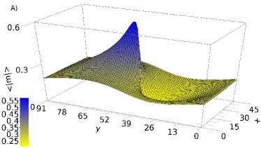
Real solids are commonly in a strained state. This can be due to a variety of reasons, ranging from forces applied upon them to the presence of structural defects, to ongoing phase transformations. Such strains affect the ordering processes of the materials Del10 ; Del09 ; Li10 ; Cah06 ; Li05 ; Dub79 . Therefore, understanding the extent of these effects is important. In this Communication, we study the continuous order-disorder phase transition in a model of a strained material. The strain field we consider results from a “wall of dislocations”, that is, a linear array of parallel edge dislocation lines. This particular arrangement of defects is relatively common in crystals, as it often occurs because of surface treatments. The resulting strain is inhomogeneous, and order develops inhomogeneously in the material, with ordered regions growing in quasi two-dimensional layers around a central cylindrical rod-shaped nucleus Del10 . Each layer orders at a different critical temperature. In order to study the critical behavior of this process, we consider a mesoscopic spin model in which the coupling between spins reflects the strain field induced by the dislocation walls. Performing several simulations of systems with different sizes and using finite size scaling, we are able to measure the critical exponents characterizing the transition. The critical exponents found are comparable with exponents that have been measured experimentally in a variety of materials, and for different types of transitions Del10 ; Del09 ; Tre98 ; Sch87 ; Tak09 ; Lom96 ; Bag93 ; Gau88 ; Bon77 ; Yel74 . Notably, similar critical exponents have recently been measured for the magnetic ordering transition that accompanies the onset of the pseudogap state in high $T_{c}$ superconductors Son09 ; Son08 ; Moo08 ; Li08 . These exponents are also compatible with those found in multicritical surface transitions Bin84 , although in our case the exponents describe bulk measurements.

Assuming that atoms interact more strongly where they are pushed closer together and more weakly where they are pulled apart, a phenomological model that captures the effect of strain on ordering due to a dislocation line can be constructed Del10 . Assuming the defects are arranged in walls extending in the $y$ direction with the lines parallel to $z$, it is found that the local relative critical temperature change $\tau_{c}(\vec{r})$ is

$$\tau_{c}\left(\vec{r}\right)\equiv\frac{T^{\prime}_{c}\left(\vec{r}\right)-T_{c}}{T_{c}}\propto\frac{b}{2l}\frac{1-2\nu}{1-\nu}\frac{\sin\left(\frac{2\pi y}{h}\right)}{\cosh\left(\frac{2\pi x}{h}\right)-\cos\left(\frac{2\pi y}{h}\right)}\>,$$ (1)

where $\vec{r}$ is the normal vector pointing from the closest dislocation line, $b$ is the magnitude of the Burgers vector, $l$ is the unit of length used, $\nu$ is Poisson’s ratio, $h$ is the local average distance between defects, $T^{\prime}_{c}\left(\vec{r}\right)$ is the local transition temperature and $T_{c}$ is the transition temperature for a defect-free crystal. This results in inhomogeneous ordering in which ordered regions nucleate and grow in the vicinity of the dislocation lines via the addition of quasi 2-D layers around nuclei with the shape of narrow cylindrical rods Del10 . Here we study the universal critical scaling properties of this ordering process.

To identify the essential physics that controls the scaling properties of this ordering behavior, we studied a zero-field 3D Ising model on a simple cubic lattice with periodic boundary conditions and nonconstant coupling $J_{ij}$ between nearest neighbor spins $i$ and $j$. The Hamiltonian is

$$\mathcal{H}=-\sum_{\left\langle ij\right\rangle}J_{ij}s_{i}s_{j}\>,$$ (2)

where $s_{i}=\pm 1$ is the value of the $i^{\mathrm{th}}$ spin and $\left\langle ij\right\rangle$ indicates sum over the nearest neighbor spins on the lattice. The spins simply represent the state of local order. The value of the coupling $J_{ij}$ is chosen in order to reflect the strain field giving rise to Eq. 1 in the following way. First note that in a “regular” Ising model, with constant coupling $J_{0}$, the critical temperature is proportional to the coupling constant:

$$J_{0}=\frac{T_{c}}{a}\>,$$ (3)

where $a$ is some proportionality constant. Also, from Eq. 1 it follows that, given a $\tau_{c}\left(\vec{r}\right)$,

$$T_{c}^{\prime}\left(\vec{r}\right)=T_{c}\left(1+\tau_{c}\left(\vec{r}\right)\right)\>.$$ (4)

Therefore, from Eqs. 3 and 4, the parts of the system that become critical at a given temperature $T_{c}^{\prime}$ are those that have a coupling

$$J(\vec{r})=\frac{T_{c}^{\prime}\left(\vec{r}\right)}{a}=\frac{T_{c}}{a}\left(1+\tau_{c}\left(\vec{r}\right)\right)=J_{0}\left(1+\tau_{c}\left(\vec{r}\right)\right)\>.$$

Thus, given the arbitrarity of $J_{0}$ and of the other proportionality constants, we set

$$J\left(\vec{r}\right)=1+\frac{\sin\left(\frac{2\pi y}{h}\right)}{\cosh\left(\frac{2\pi x}{h}\right)-\cos\left(\frac{2\pi y}{h}\right)}\>,$$

where we take $h$ to be the size of the system in the $y$ direction. To reproduce the effects of the strain of a wall, we use the above expression only for the coupling between spins in the $x$ and $y$ directions, while we set the coupling of the spins along $z$ at 1. The simulated systems contained a single dislocation line in the center. The replicas due to the periodic boundary conditions used effectively turned it into a wall of lines. Notice that while the strain field due to a single dislocation line is long-range, the one due to a wall is short-ranged Del10 . However, the field of a wall maintains the dipole-like nature of the field of a single line, with the effect of promoting the order on one side of the system, while suppressing it on the other. The order parameter in our simulations was given by the ensemble averaged absolute value of the magnetization per spin:

$$\left\langle\left|m\right|\right\rangle=\frac{1}{N}\left|\sum_{i}s_{i}\right|\>,$$

where $N$ is the total number of spins.

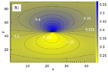
Using the Wolff algorithm Wol89 , which is a cluster flipping algorithm Swe87 , we performed extensive Monte Carlo simulations of this model. The cylindrical ordered regions grow with decreasing temperature as the surfaces of the cylinders order in a fashion consistent with earlier predictions Del10 . Figure 1 shows the order parameter in an $x$-$y$ cross section of a $45\times 91\times 40$ system, averaged over $z$, at a temperature of $4.49$ in units of the Boltzmann constant $k_{B}$. As anticipated, order is increasingly enhanced with proximity to the dislocation line on one half of the system. On the other half, instead, order is increasingly suppressed. Also notice that the contour lines closely follow the predicted shape, shown in Fig. 6 of Ref. Del10, and computed by numerically solving the following parametric equations for a particular value of $\tau_{c}$:

$$y\left(x\right)=\frac{h}{\pi}\arctan\left\{\frac{\pi\pm\sqrt{\pi^{2}+\tau_{c}^{2}\left[1-\cosh^{2}\left(\frac{2\pi x}{h}\right)\right]}}{\tau_{c}\left[\cosh\left(\frac{2\pi x}{h}\right)+1\right]}\right\}\>;$$

$$x\left(y\right)=\pm\frac{h}{2\pi}\operatorname{arccosh}\left\{\frac{2\pi\tan\left(\frac{\pi y}{h}\right)+\tau_{c}\left[1-\tan^{2}\left(\frac{\pi y}{h}\right)\right]}{\tau_{c}\left[1+\tan^{2}\left(\frac{\pi y}{h}\right)\right]}\right\}\>.$$

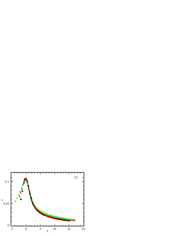
We find that the ordering occurs via a continuous transition. To measure the critical exponents, we simulated systems of different sizes and estimated their values using finite size scaling New99 . The observables measured were the magnetization order parameter and the ensemble averaged total energy, given by Eq. 2. From the fluctuations of magnetization and energy we also calculated the magnetic susceptibility $\chi$ and the specific heat $c$. The measurements were taken at the same time over the entire system and over an arbitrarily chosen quasi two-dimensional layer, corresponding to a fixed, chosen value of $\tau_{c}$. For each value of the temperature we took ensemble averages over a number of system updates between $10^{6}$ and $10^{8}$. The whole system sizes were $59\times 23\times 13$, $109\times 43\times 25$, and $205\times 83\times 50$, while the circumferences of the $x$-$y$ cross sections of the quasi two-dimensional layers measured were 50, 102 and 200, corresponding to $\tau_{c}=0.9$. The sizes of the systems in the $x$ direction were chosen so that the coupling between spins was within $10^{-6}$ of unity at the boundaries.

To perform data collapses using finite size scaling, we define the scaled reduced temperature $\tilde{t}$ as

$$\tilde{t}\left(t\right)=L^{1/\nu}t\>,$$

where $L$ is the length of the largest dimension of the system considered, which in our case corresponds to the length in the $x$ direction, $\nu$ is the correlation length critical exponent and $t\equiv\frac{T-T_{c}}{T_{c}}$ is the reduced temperature. With this definition of $\tilde{t}$, the scaling functions for the order parameter, the magnetic susceptibility and the specific heat are, respectively,

$$\langle|\tilde{m}|\rangle\left(\tilde{t}\right)=L^{\beta/\nu}\langle|m|\rangle\left(\tilde{t}\right)\>,$$

$$\tilde{\chi}\left(\tilde{t}\right)=L^{-\gamma/\nu}\chi\left(\tilde{t}\right)\>,$$

$$\tilde{c}\left(\tilde{t}\right)=L^{-\alpha/\nu}c\left(\tilde{t}\right)\>,$$

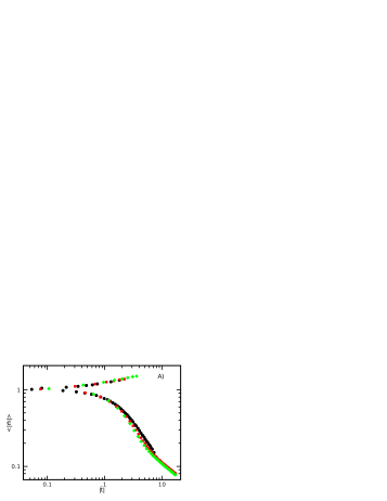
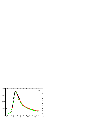
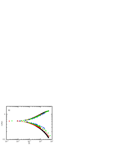
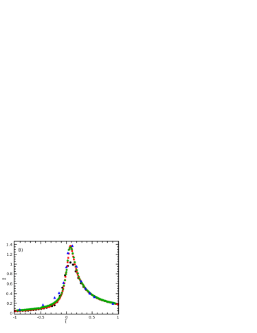
where $\beta$, $\gamma$ and $\alpha$ are the corresponding critical exponents. The data collapses for the quasi two-dimensional layer, shown in Fig. 2, allow estimates of the critical indices of $\beta=0.18\pm 0.02$, $\gamma=1.0\pm 0.1$, $\alpha=0.10\pm 0.02$ and $\nu=2.0\pm 0.1$, with a critical temperature of $6.7\pm 0.2$. The errors were conservatively estimated as the range over which a reasonable scaling collapse was achieved.

Similarly, the measurements of the whole systems, whose data collapses are shown in Fig. 3, allow the values of the critical exponents to be estimated as $\beta=0.18\pm 0.02$, $\gamma=1.1\pm 0.2$ and $\nu=2.0\pm 0.25$, with a critical temperature of $4.50\pm 0.05$. We could not produce a good scaling collapse for the specific heat. Note that we get essentially the same exponents for the whole system that we do for the quasi two-dimensional layer. This reveals that the nature of the transition of the whole system is essentially the same as that of a quasi two-dimensional layer. At any given temperature, there is a part of the system that is critical. The biggest of these parts corresponds to the measured critical temperature for the whole system. Also notice that the susceptibility for the smallest system does not scale well near the peak, presumably due to finite size effects. The size of the error bars on the data shown in Figs. 2 and 3 is substantially smaller than the size of the symbols.

The exponents characterizing the transition are compatible with those corresponding to the, so-called, “special” multicritical point in surface critical phenomena. In particular, the value $\beta=0.18$ was reported in Refs. Bin84 and Lan90 and is consistent with prior theoretical calculations based on scaling Ree81 ; Bin84 . Also, the measured mean-field value of the exponent $\gamma=1$ is expected at the multicritical point Bin74 . Furthermore, using the “bulk” 3d-Ising value for the critical exponent $\nu=0.632$ in the scaling laws, as in Ref. Bin84 , the hyperscaling relation predicts $\alpha=0.104$, which is compatible with the one we measured. Note, however, that while these previous studies considered systems with an actual surface, our model does not have free layers. In fact, the quasi two-dimensional layers whose ordering we studied are in the midst of of the system. Nevertheless, the ordering in our system does occur in a quasi two-dimensional layer at the surface of the already ordered region.

Similar exponents have also been measured for a number of different types of transitions in a variety of physical systems, ranging from structural transitions, to the percolation of excitons in polymeric matrices, to magnetic order in frustrated materials Del10 ; Del09 ; Tre98 ; Sch87 ; Tak09 ; Lom96 ; Bag93 ; Gau88 ; Bon77 ; Yel74 . In particular, as mentioned earlier, there have been recent observations of magnetic ordering at the onset of the pseudogap transition in high-$T_{c}$ superconductors in which similar critical exponents have been measured Son09 ; Son08 ; Moo08 ; Li08 . Given the scale invariant nature of critical phenomena, the fact that the phase transition in our model apparently has the same set of critical exponents suggests that the essential physics is the same in both systems, and that our results may be relevant to the open question of the nature of the pseudogap state itself. Intriguingly, recent experiments have shown that the onset of the pseudogap state is accompanied by local modulations of atomic displacement that generate significant inhomogeneous strains Isl02 ; Isl04 . This suggests that, like the quasi two-dimensional ordering process we have considered, the pseudogap transition occurs because of inhomogeneous strain.

Assuming this is true and noting that the pseudogap transition precedes the onset of high-$T_{c}$ superconductivity Moo08 , it appears that some strain is required for the development of high-$T_{c}$ superconductivity. However, strain is also known to adversely affect superconductivity Cal04 ; Bus04 ; Zhu03 ; Jan03 and too much strain supresses it altogether Li08 . The optimal doping concentration of the high-$T_{c}$ superconductor YBa_2Cu_3O_7-$\delta$ occurs at only $\delta\approx 0.08$. Such a small deviation from an exact stoichiometry presumably introduces enough strain to cause a pseudogap transition while causing only minor adverse effects. This supports the idea that the pseudogap state is a physically direct precursor to superconductivity, even though its cause competes with it, consistent with some of the original ideas concerning the mechanism of high-temperature superconductivity Eme87 ; Eme95 .