Meromorphic Lévy processes and their fluctuation identities

A. Kuznetsov 111Department of Mathematics and Statistics, York University, 4700 Keele Street, Toronto, Ontario, M3J 1P3, Canada. Email: kuznetsov@mathstat.yorku.ca ,  A. E. Kyprianou 222Department of Mathematical Sciences, University of Bath, Claverton Down, Bath, BA2 7AY, U.K.. Email: a.kyprianou@bath.ac.uk ,   J. C. Pardo 333Centro de Investigación en Matemáticas A.C. Calle Jalisco s/n. 36240 Guanajuato, México. Email: jcpardo@cimat.mx
(This version: )
Abstract

The last couple of years has seen a remarkable number of new, explicit examples of the Wiener-Hopf factorization for Lévy processes where previously there had been very few. We mention in particular the many cases of spectrally negative Lévy processes in [21, 32], hyper-exponential and generalized hyper-exponential Lévy processes [24], Lamperti-stable processes in [9, 10, 13, 39], Hypergeometric processes in [35, 31, 11], β𝛽\beta-processes in [29] and θ𝜃\theta-processes in [30].

In this paper we introduce a new family of Lévy processes, which we call Meromorphic Lévy processes, or just M𝑀M-processes for short, which overlaps with many of the aforementioned classes. A key feature of the M𝑀M-class is the identification of their Wiener-Hopf factors as rational functions of infinite degree written in terms of poles and roots of the Laplace exponent, all of which are real numbers. The specific structure of the M𝑀M-class Wiener-Hopf factorization enables us to explicitly handle a comprehensive suite of fluctuation identities that concern first passage problems for finite and infinite intervals for both the process itself as well as the resulting process when it is reflected in its infimum. Such identities are of fundamental interest given their repeated occurrence in various fields of applied probability such as mathematical finance, insurance risk theory and queuing theory.


Keywords: Lévy processes, Wiener-Hopf factorization, exit problems, fluctuation theory.

AMS 2000 subject classifications: 60G51, 60G50.

1 Introduction

The theory of Lévy processes forms the cornerstone of an enormous volume of mathematical literature which supports a wide variety of applied and theoretical stochastic models. One of the most obvious and fundamental problems that can be stated for a Lévy process, particularly in relation to its role as a modelling tool, is the distributional characterization of the time at which a Lévy process first exists either an infinite or finite interval together with its overshoot beyond the boundary of the interval. As a family of stochastic processes, Lévy processes are now well understood and the exit problem has seen many different approaches dating back to the 1960s. See for example [2, 6, 8, 16, 41, 19, 13, 35] to name but a few.

Despite the maturity of this field of study it is surprising to note that, until very recently, there were less than a handful of examples for which explicit analytical detail concerning the first exit problem could be explored. Given the closeness in mathematical proximity of the first exit problem to the characterization of the Wiener-Hopf factorization, one might argue that the lack of concrete examples of the former was a consequence of the same being true for the latter. The landscape for both the Wiener-Hopf factorization problem and the first exit problem has changed quite rapidly in the last couple of years however with the discovery of a number of new, mathematically tractable families of Lévy processes. We mention in particular the many cases of spectrally negative Lévy processes in [21, 32], hyper-exponential and generalized hyper-exponential Lévy processes [24], Lamperti-stable processes in [9, 10, 13], Hypergeometric processes in [35, 31], β𝛽\beta-processes in [29] and θ𝜃\theta-processes in [30].

In this paper we introduce a new family of Lévy processes, which we call Meromorphic Lévy processes, or just M𝑀M-class for short, that overlaps with many of the aforementioned classes. Our definition of the M𝑀M-class of processes will allow us to drive features of their Wiener-Hopf factors through to many of the fluctuation identities which are of pertinence for a wide variety of applications. In the theory of actuarial mathematics, the problem of first exit from a half-line is of fundamental interest with regard to the classical ruin problem and is typically studied within the context of an expected discounted penalty function. The latter is also known as the Gerber-Shiu function following the first article [18] of a long series of papers found within the actuarial literature. In the setting of financial mathematics, the first exit of a Lévy process, as well as a Lévy process reflected in its infimum, from an interval is of interest in the pricing of barrier options and American-type options, [1], as well as certain credit risk models, [20, 33]. In queueing theory exit problems for Lévy processes play a central role in understanding the trajectory of the workload during busy periods as well as in relation to buffers, [17, 27]. Many optimal stopping strategies also turn out to boil down to first passage problems for both Lévy processes and Lévy processes reflected in their infimum; classic examples of which include McKean’s optimal stopping problem, [38], as well as the Shepp-Shiryaev optimal stopping problem, [2, 3] .

It is not our purpose however to dwell on these applications. As alluded to above, the main objective will be expose a comprehensive suite of fluctuation identities in explicit form for the M𝑀M-class of Lévy processes. We thus conclude the introduction with an overview of the paper.


In the next section we give a formal definition of meromorphic Lévy processes, dwelling in particular on their relationship with discrete completely monotone functions. In Section 3 we consider several classes of existing families of Lévy processes that have appeared in recent literature. Next, in Section 4 we establish explicit identities for the exponentially discounted first passage problem. In particular we deal with (what is known in the actuarial literature as) the Gerber-Shiu measure describing the discounted joint triple law of the overshoot, undershoot and undershoot of the maximum at first passage over a level as well as the marginal thereof which specifies the law of the discounted overshoot. It is important to note that the discounting factor which appears in all of the identities means that one is never more than a Fourier transform away from the naturally associated space-time identity in which the additional law of the time to first passage is specified. This last Fourier inversion appears to be virtually impossible to produce analytically within the current context, but the expressions we offer are not difficult to work with in conjunction with straightforward Fourier inversion algorithms.

In Section 5 we look at the more complicated two-sided exit problem. Inspired by a technique of Rogozin [41] we solve a system of equations which characterize the discounted overshoot distribution on either side of the interval in question. The same technique also delivers explicit expressions for the discounted entrance law into an interval. In Section 6 we look in analytical detail at what can be said of the ascending and descending ladder variables. In particular we offer expressions for their joint Laplace exponent and jump measure. Section 7 mentions some additional examples of fluctuation identities which enjoy explicit detail and finally in Section 8 we describe some numerical experiments in order to exhibit the genuine practical applicability of our method.

2 Meromorphic Lévy processes

Recall that a general one-dimensional Lévy process is a stochastic process issued from the origin with stationary and independent increments and almost sure right continuous paths. We write X={Xt:t0}𝑋conditional-setsubscript𝑋𝑡𝑡0X=\{X_{t}:t\geq 0\} for its trajectory and \mathbb{P} for its law. As X𝑋X is necessarily a strong Markov process, for each x𝑥x\in\mathbb{R}, we will need the probability xsubscript𝑥\mathbb{P}_{x} to denote the law of X𝑋X when issued from x𝑥x with the understanding that 0=subscript0\mathbb{P}_{0}=\mathbb{P}. The law \mathbb{P} of Lévy processes is characterized by its one-time transition probabilities. In particular there always exist a triple (a,σ,Π)𝑎𝜎Π(a,\sigma,\Pi) where a𝑎a\in\mathbb{R}, σ𝜎\sigma\in\mathbb{R} and ΠΠ\Pi is a measure on \{0}\0\mathbb{R}\backslash\{0\} satisfying the integrability condition (1x2)Π(dx)<subscript1superscript𝑥2Πd𝑥\int_{\mathbb{R}}(1\wedge x^{2})\Pi({\rm d}x)<\infty, such that, for all z𝑧z\in\mathbb{R}

𝔼[eizXt]=etψ(iz),𝔼delimited-[]superscript𝑒i𝑧subscript𝑋𝑡superscript𝑒𝑡𝜓i𝑧\displaystyle\mathbb{E}[e^{{\textnormal{i}}zX_{t}}]=e^{t\psi({\textnormal{i}}z)}, (1)

where the Laplace exponent ψ(z)𝜓𝑧\psi(z) is given by the Lévy-Khintchine formula

ψ(z)=12σ2z2+μz+(ezx1zxh(x))Π(dx).𝜓𝑧12superscript𝜎2superscript𝑧2𝜇𝑧subscriptsuperscript𝑒𝑧𝑥1𝑧𝑥𝑥Πd𝑥\displaystyle\psi(z)=\frac{1}{2}\sigma^{2}z^{2}+\mu z+\int_{\mathbb{R}}\left(e^{zx}-1-zxh(x)\right)\Pi({\rm d}x). (2)

Here h(x)𝑥h(x) is the cutoff function which is usually taken to be h(x)𝕀{|x|<1}𝑥subscript𝕀𝑥1h(x)\equiv{\mathbb{I}}_{\{|x|<1\}}. However, everywhere in the present paper we will work with the Lévy measures Π(dx)Πd𝑥\Pi({\textnormal{d}}x) which have exponentially decaying tails, thus we will take h(x)1𝑥1h(x)\equiv 1. Note, that the exponential decay of the tails of the Lévy measure also implies that the Laplace exponent can be analytically continued into some vertical strip a<Re(z)<b𝑎Re𝑧𝑏a<\textnormal{Re}(z)<b for a<0<b𝑎0𝑏a<0<b.

Everywhere in this paper we will denote the tails of the Lévy measure as Π¯+(x)=Π((x,))superscript¯Π𝑥Π𝑥\bar{\Pi}^{+}(x)=\Pi((x,\infty)) and Π¯(x)=Π((,x))superscript¯Π𝑥Π𝑥\bar{\Pi}^{-}(x)=\Pi((-\infty,-x)) for x>0𝑥0x>0. Let us define the supremum/infimum processes X¯t=supstXssubscript¯𝑋𝑡subscriptsupremum𝑠𝑡subscript𝑋𝑠\overline{X}_{t}=\sup_{s\leq t}X_{s}, X¯t=infstXssubscript¯𝑋𝑡subscriptinfimum𝑠𝑡subscript𝑋𝑠\underline{X}_{t}=\inf_{s\leq t}X_{s} and denote by e(q)e𝑞{\textnormal{e}}(q) an independent, exponentially distributed random variable with rate q>0𝑞0q>0. Finally, the first passage time above x𝑥x is defined as τx+=inf{t>0:Xt>x}superscriptsubscript𝜏𝑥infimumconditional-set𝑡0subscript𝑋𝑡𝑥\tau_{x}^{+}=\inf\{t>0:X_{t}>x\}, and similarly τy=inf{t>0:Xt<y}superscriptsubscript𝜏𝑦infimumconditional-set𝑡0subscript𝑋𝑡𝑦\tau_{y}^{-}=\inf\{t>0:X_{t}<y\}.

Let us recall some basic facts about completely monotone functions. A function f:(0,):𝑓maps-to0f:(0,\infty)\mapsto{\mathbb{R}} is called completely monotone if f𝒞𝑓superscript𝒞f\in{\mathcal{C}}^{\infty} and (1)nf(n)(x)0superscript1𝑛superscript𝑓𝑛𝑥0(-1)^{n}f^{(n)}(x)\geq 0 for all n{0}𝑛0n\in{\mathbb{N}}\cup\{0\} and x>0𝑥0x>0. According to Bernstein theorem (see Theorem 1.4 in [42]), the function f𝑓f is completely monotone if and only if it can be represented as the Laplace transform of a positive measure on [0,)0[0,\infty):

f(x)=[0,)ezxμ(dz),x>0.formulae-sequence𝑓𝑥subscript0superscript𝑒𝑧𝑥𝜇d𝑧𝑥0\displaystyle f(x)=\int\limits_{[0,\infty)}e^{-zx}\mu({\textnormal{d}}z),\;\;\;x>0. (3)

Note that if f(0+)=1𝑓superscript01f(0^{+})=1, then μ(dx)𝜇d𝑥\mu({\textnormal{d}}x) is a probability measure and 1f(x)1𝑓𝑥1-f(x) is the cumulative distribution function of a positive infinitely divisible random variable Z𝑍Z, whose distribution is a mixture of exponential distributions. We will denote the class of completely monotone functions as 𝒞𝒞{\mathcal{CM}}.

Next, let us introduce a subclass of completely monotone functions, which will be important for us later. We will call f:(0,):𝑓maps-to0f:(0,\infty)\mapsto{\mathbb{R}} a discrete completely monotone function if the measure μ(dz)𝜇d𝑧\mu({\textnormal{d}}z) in the representation (3) is discrete, and the support of the measure μ(dz)𝜇d𝑧\mu({\textnormal{d}}z) is infinite and does not have finite accumulation points. This implies that the measure μ(dz)𝜇d𝑧\mu({\textnormal{d}}z) is an infinite mixture of atoms of size ansubscript𝑎𝑛a_{n} at the points bnsubscript𝑏𝑛b_{n}

μ(dz)=n1anδbn(dz),𝜇d𝑧subscript𝑛1subscript𝑎𝑛subscript𝛿subscript𝑏𝑛d𝑧\displaystyle\mu({\textnormal{d}}z)=\sum\limits_{n\geq 1}a_{n}\delta_{b_{n}}({\textnormal{d}}z),

where δb(dx)subscript𝛿𝑏d𝑥\delta_{b}({\textnormal{d}}x) denotes the Dirac measure at x=b𝑥𝑏x=b, for all n1𝑛1n\geq 1 we have an>0subscript𝑎𝑛0a_{n}>0, bn0subscript𝑏𝑛0b_{n}\geq 0 and bnsubscript𝑏𝑛b_{n}\to\infty as n𝑛n\to\infty (without loss of generality we can also assume that the sequence {bn}n1subscriptsubscript𝑏𝑛𝑛1\{b_{n}\}_{n\geq 1} is strictly increasing). From (3) it follows then that any discrete completely monotone function can be represented as an infinite series of exponential functions

f(x)=n1anebnx,x>0.formulae-sequence𝑓𝑥subscript𝑛1subscript𝑎𝑛superscript𝑒subscript𝑏𝑛𝑥𝑥0\displaystyle f(x)=\sum\limits_{n\geq 1}a_{n}e^{-b_{n}x},\;\;\;x>0. (4)

We will denote the class of discrete completely monotone functions as 𝒟𝒞𝒟𝒞{\mathcal{DCM}}.

Definition 1 (M𝑀M-class).

A Lévy process X𝑋X is said to belong to the Meromorophic class (M𝑀M-class) if Π¯+(x),Π¯(x)𝒟𝒞superscript¯Π𝑥superscript¯Π𝑥𝒟𝒞\bar{\Pi}^{+}(x),\bar{\Pi}^{-}(x)\in{\mathcal{DCM}}.

We see that according to our definition of the discrete completely monotone functions, the process is Meromorphic if and only if the Lévy measure Π(dx)Πd𝑥\Pi({\textnormal{d}}x) has a density with respect to the Lebesgue measure, given by

π(x)=𝕀{x>0}n1anρneρnx+𝕀{x<0}n1a^nρ^neρ^nx,𝜋𝑥subscript𝕀𝑥0subscript𝑛1subscript𝑎𝑛subscript𝜌𝑛superscript𝑒subscript𝜌𝑛𝑥subscript𝕀𝑥0subscript𝑛1subscript^𝑎𝑛subscript^𝜌𝑛superscript𝑒subscript^𝜌𝑛𝑥\displaystyle\pi(x)={\mathbb{I}}_{\{x>0\}}\sum\limits_{n\geq 1}a_{n}\rho_{n}e^{-\rho_{n}x}+{\mathbb{I}}_{\{x<0\}}\sum\limits_{n\geq 1}\hat{a}_{n}\hat{\rho}_{n}e^{\hat{\rho}_{n}x}, (5)

where all the coefficients ansubscript𝑎𝑛a_{n}, a^nsubscript^𝑎𝑛\hat{a}_{n}, ρnsubscript𝜌𝑛\rho_{n}, ρ^nsubscript^𝜌𝑛\hat{\rho}_{n} are positive, the sequences {ρn}n1subscriptsubscript𝜌𝑛𝑛1\{\rho_{n}\}_{n\geq 1} and {ρ^n}n1subscriptsubscript^𝜌𝑛𝑛1\{\hat{\rho}_{n}\}_{n\geq 1} are stricly increasing, and ρn+subscript𝜌𝑛\rho_{n}\to+\infty and ρ^n+subscript^𝜌𝑛\hat{\rho}_{n}\to+\infty as n+𝑛n\to+\infty.

Proposition 1.

Assume that π(x)𝜋𝑥\pi(x) is given by (5). The integral x2π(x)dxsubscriptsuperscript𝑥2𝜋𝑥d𝑥\int_{{\mathbb{R}}}x^{2}\pi(x){\textnormal{d}}x converges if and only if both series n1anρn2subscript𝑛1subscript𝑎𝑛superscriptsubscript𝜌𝑛2\sum_{n\geq 1}a_{n}\rho_{n}^{-2} and n1a^nρ^n2subscript𝑛1subscript^𝑎𝑛superscriptsubscript^𝜌𝑛2\sum_{n\geq 1}\hat{a}_{n}\hat{\rho}_{n}^{-2} converge.

Proof.

The ”if” part was established in Proposition 1 in [30]. The ”only if” part follows from (5) and the Monotone Convergence Theorem. square-intersectionsquare-union\sqcap\kern-8.0pt\hbox{$\sqcup$}

Recall, that a function g:{}:𝑔maps-tog:{\mathbb{C}}\mapsto{\mathbb{C}}\cup\{\infty\} is called meromorphic if it does not have any other singularities in the open complex plane except for poles. A function g(z)𝑔𝑧g(z) is called real meromorphic function if it is meromorphic and g(z){}𝑔𝑧g(z)\in{\mathbb{R}}\cup\{\infty\} for all z𝑧z\in{\mathbb{R}}, or equivalently, if g(z)¯=g(z¯)¯𝑔𝑧𝑔¯𝑧{\overline{g(z)}}=g(\bar{z}).

Theorem 1.

The following conditions are equivalent:

  • (i)

    X𝑋X is Meromorphic.

  • (ii)

    Π¯+(x),Π¯(x)𝒞superscript¯Π𝑥superscript¯Π𝑥𝒞\bar{\Pi}^{+}(x),\bar{\Pi}^{-}(x)\in{\mathcal{CM}} and the Laplace exponent ψ(z)𝜓𝑧\psi(z) is meromorphic.

  • (iii)

    For some q>0𝑞0q>0 (and then, for every q>0𝑞0q>0) the functions (X¯e(q)>x)subscript¯𝑋e𝑞𝑥{\mathbb{P}}({\overline{X}}_{{\textnormal{e}}(q)}>x) and (X¯e(q)>x)subscript¯𝑋e𝑞𝑥{\mathbb{P}}(-{\underline{X}}_{{\textnormal{e}}(q)}>x) restricted to x>0𝑥0x>0 belong to the class 𝒟𝒞𝒟𝒞{\mathcal{DCM}}.

  • (iv)

    For some q>0𝑞0q>0 (and then, for every q>0𝑞0q>0) the functions (Xe(q)>x)subscript𝑋e𝑞𝑥{\mathbb{P}}(X_{{\textnormal{e}}(q)}>x) and (Xe(q)>x)subscript𝑋e𝑞𝑥{\mathbb{P}}(-X_{{\textnormal{e}}(q)}>x) restricted to x>0𝑥0x>0 belong to the class 𝒟𝒞𝒟𝒞{\mathcal{DCM}}.

  • (v)

    For some q>0𝑞0q>0 (and then, for every q>0𝑞0q>0) we have the factorization

    qψ(z)=qn11zζn1zρnn11+zζ^n1+zρ^n,z,formulae-sequence𝑞𝜓𝑧𝑞subscriptproduct𝑛11𝑧subscript𝜁𝑛1𝑧subscript𝜌𝑛subscriptproduct𝑛11𝑧subscript^𝜁𝑛1𝑧subscript^𝜌𝑛𝑧\displaystyle q-\psi(z)=q\prod\limits_{n\geq 1}\frac{1-\frac{z}{\zeta_{n}}}{1-\frac{z}{\rho_{n}}}\prod\limits_{n\geq 1}\frac{1+\frac{z}{\hat{\zeta}_{n}}}{1+\frac{z}{\hat{\rho}_{n}}},\;\;\;z\in{\mathbb{C}}, (6)

    where all roots {ζn,ζ^n}subscript𝜁𝑛subscript^𝜁𝑛\{\zeta_{n},-\hat{\zeta}_{n}\} of ψ(z)q𝜓𝑧𝑞\psi(z)-q are real and interlace with the poles {ρn,ρ^n}subscript𝜌𝑛subscript^𝜌𝑛\{\rho_{n},-\hat{\rho}_{n}\}

    ρ^2<ζ^2<ρ^1<ζ^1<0<ζ1<ρ1<ζ2<ρ2<subscript^𝜌2subscript^𝜁2subscript^𝜌1subscript^𝜁10subscript𝜁1subscript𝜌1subscript𝜁2subscript𝜌2\displaystyle...-\hat{\rho}_{2}<-\hat{\zeta}_{2}<-\hat{\rho}_{1}<-\hat{\zeta}_{1}<0<\zeta_{1}<\rho_{1}<\zeta_{2}<\rho_{2}<... (7)
  • (vi)

    The Laplace exponent ψ(z)𝜓𝑧\psi(z) is a real meromorphic function, which satisfies Im(ψ(z)/z)>0Im𝜓𝑧𝑧0\textnormal{Im}(\psi(z)/z)>0 for all z𝑧z in the half-plane Im(z)>0Im𝑧0\textnormal{Im}(z)>0.

Proof.

The main ideas and tools needed for the proof of this theorem come from the proofs of Theorem 2 in [40] and Theorem 1 in [30].

(i)\Rightarrow(ii) Using (5) and (2) we find that

ψ(z)=12σ2z2+μz+z2n1anρn(ρnz)+z2n1a^nρ^n(ρ^n+z),z,formulae-sequence𝜓𝑧12superscript𝜎2superscript𝑧2𝜇𝑧superscript𝑧2subscript𝑛1subscript𝑎𝑛subscript𝜌𝑛subscript𝜌𝑛𝑧superscript𝑧2subscript𝑛1subscript^𝑎𝑛subscript^𝜌𝑛subscript^𝜌𝑛𝑧𝑧\displaystyle\psi(z)=\frac{1}{2}\sigma^{2}z^{2}+\mu z+z^{2}\sum\limits_{n\geq 1}\frac{a_{n}}{\rho_{n}(\rho_{n}-z)}+z^{2}\sum\limits_{n\geq 1}\frac{\hat{a}_{n}}{\hat{\rho}_{n}(\hat{\rho}_{n}+z)},\;\;\;z\in{\mathbb{C}}, (8)

which shows that ψ(z)𝜓𝑧\psi(z) is a meromorphic function. Since 𝒟𝒞𝒞𝒟𝒞𝒞{\mathcal{DCM}}\subset{\mathcal{CM}} this proves (ii).

(ii)\Rightarrow(vi) We know that ψ(z)𝜓𝑧\psi(z) is a meromorphic function, and that ψ(0)=0𝜓00\psi(0)=0, therefore ψ(z)𝜓𝑧\psi(z) is analytic in some neighbourhood of zero. From the proof of Theorem 2 in [40] we find that (a) ψ(z)𝜓𝑧\psi(z) can be analytically continued in the half-planes Im(z)>0Im𝑧0\textnormal{Im}(z)>0 and Im(z)<0Im𝑧0\textnormal{Im}(z)<0, (b) Im(ψ(z)/z)>0Im𝜓𝑧𝑧0\textnormal{Im}(\psi(z)/z)>0 for all z𝑧z in the half-plane Im(z)>0Im𝑧0\textnormal{Im}(z)>0. Since ψ(z)¯=ψ(z¯)¯𝜓𝑧𝜓¯𝑧\overline{\psi(z)}=\psi(\bar{z}) we conclude that ψ(z)𝜓𝑧\psi(z) is a real meromorphic function. Using this fact and the above statement (b) we obtain (vi).

(vi)\Rightarrow(v), q>0for-all𝑞0\forall q>0. For q>0𝑞0q>0 and Im(z)>0Im𝑧0\textnormal{Im}(z)>0 it is true that Im(q/z)>0Im𝑞𝑧0\textnormal{Im}(-q/z)>0, thus (vi) implies that Im((ψ(z)q)/z)>0Im𝜓𝑧𝑞𝑧0\textnormal{Im}((\psi(z)-q)/z)>0 for all z𝑧z in the half-plane Im(z)>0Im𝑧0\textnormal{Im}(z)>0. Using Theorem 1 on page 220 in [36] (the statement of this result can also be found in the proof of Theorem 1 in [30]) we find that (v) is valid for all q>0𝑞0q>0.

(v)\Rightarrow(iii) This follows from Theorem 1 in [30].

(iii)\Rightarrow(iv) One can also check that if two functions f(x)𝑓𝑥f(x) and g(x)𝑔𝑥g(-x) belong to the class 𝒟𝒞𝒟𝒞{\mathcal{DCM}}, then the same is true for 𝕀{x>0}(fg)(x)subscript𝕀𝑥0𝑓𝑔𝑥{\mathbb{I}}_{\{x>0\}}(f*g)(x) and 𝕀{x<0}(fg)(x)subscript𝕀𝑥0𝑓𝑔𝑥{\mathbb{I}}_{\{x<0\}}(f*g)(x), where fg𝑓𝑔f*g is the convolution. The result (iv) then follows easily from this fact and the Wiener-Hopf decomposition which says that Xe(q)=dY1+Y2superscript𝑑subscript𝑋e𝑞subscript𝑌1subscript𝑌2X_{{\textnormal{e}}(q)}\stackrel{{\scriptstyle d}}{{=}}Y_{1}+Y_{2}, where the random variables Y1subscript𝑌1Y_{1} and Y2subscript𝑌2Y_{2} are independent, Y1=dX¯e(q)superscript𝑑subscript𝑌1subscript¯𝑋e𝑞Y_{1}\stackrel{{\scriptstyle d}}{{=}}{\overline{X}}_{{\textnormal{e}}(q)} and Y2=dX¯e(q)superscript𝑑subscript𝑌2subscript¯𝑋e𝑞Y_{2}\stackrel{{\scriptstyle d}}{{=}}{\underline{X}}_{{\textnormal{e}}(q)}.

(iv)\Rightarrow(i) From (iv) and the definition of the 𝒟𝒞𝒟𝒞{\mathcal{DCM}} class we know that for some q>0𝑞0q>0 there exist α00subscript𝛼00\alpha_{0}\geq 0 and positive constants αnsubscript𝛼𝑛\alpha_{n}, βnsubscript𝛽𝑛\beta_{n}, α^nsubscript^𝛼𝑛\hat{\alpha}_{n}, β^nsubscript^𝛽𝑛\hat{\beta}_{n} such that

(Xe(q)dx)=α0δ0(dx)+[𝕀{x>0}n1αnβn1eβnx+𝕀{x<0}n1α^nβ^n1eβ^nx]dx.subscript𝑋e𝑞d𝑥subscript𝛼0subscript𝛿0d𝑥delimited-[]subscript𝕀𝑥0subscript𝑛1subscript𝛼𝑛superscriptsubscript𝛽𝑛1superscript𝑒subscript𝛽𝑛𝑥subscript𝕀𝑥0subscript𝑛1subscript^𝛼𝑛superscriptsubscript^𝛽𝑛1superscript𝑒subscript^𝛽𝑛𝑥d𝑥\displaystyle{\mathbb{P}}(X_{{\textnormal{e}}(q)}\in{\textnormal{d}}x)=\alpha_{0}\delta_{0}({\textnormal{d}}x)+\left[{\mathbb{I}}_{\{x>0\}}\sum\limits_{n\geq 1}\alpha_{n}\beta_{n}^{-1}e^{-\beta_{n}x}+{\mathbb{I}}_{\{x<0\}}\sum\limits_{n\geq 1}\hat{\alpha}_{n}\hat{\beta}_{n}^{-1}e^{\hat{\beta}_{n}x}\right]{\textnormal{d}}x. (9)

Note that the condition (Xe(q))=1subscript𝑋e𝑞1{\mathbb{P}}(X_{{\textnormal{e}}(q)}\in{\mathbb{R}})=1 implies that both series n1αnβn2subscript𝑛1subscript𝛼𝑛superscriptsubscript𝛽𝑛2\sum_{n\geq 1}\alpha_{n}\beta_{n}^{-2} and n1α^nβ^n2subscript𝑛1subscript^𝛼𝑛superscriptsubscript^𝛽𝑛2\sum_{n\geq 1}\hat{\alpha}_{n}\hat{\beta}_{n}^{-2} converge. Let us define ψ~(z)=z2𝔼[exp(zXe(q))]~𝜓𝑧superscript𝑧2𝔼delimited-[]𝑧subscript𝑋e𝑞\tilde{\psi}(z)=z^{2}{\mathbb{E}}[\exp(zX_{{\textnormal{e}}(q)})]. Using (9) we obtain

ψ~(z)=α0z2+z2n1αnβn(βnz)+z2n1α^nβ^n(β^n+z),z.formulae-sequence~𝜓𝑧subscript𝛼0superscript𝑧2superscript𝑧2subscript𝑛1subscript𝛼𝑛subscript𝛽𝑛subscript𝛽𝑛𝑧superscript𝑧2subscript𝑛1subscript^𝛼𝑛subscript^𝛽𝑛subscript^𝛽𝑛𝑧𝑧\displaystyle\tilde{\psi}(z)=\alpha_{0}z^{2}+z^{2}\sum\limits_{n\geq 1}\frac{\alpha_{n}}{\beta_{n}(\beta_{n}-z)}+z^{2}\sum\limits_{n\geq 1}\frac{\hat{\alpha}_{n}}{\hat{\beta}_{n}(\hat{\beta}_{n}+z)},\;\;\;z\in{\mathbb{C}}.

Comparing the above formula with (8) we conclude that ψ~(z)~𝜓𝑧\tilde{\psi}(z) is a Laplace exponent of a Meromorphic Lévy process. We have already proved that (i) implies (vi), therefore Im(ψ~(z)/z)>0Im~𝜓𝑧𝑧0\textnormal{Im}(\tilde{\psi}(z)/z)>0 for all z𝑧z in the half-plane Im(z)>0Im𝑧0\textnormal{Im}(z)>0.

Next, using the definition of the Laplace exponent (1) it is easy to verify that 𝔼[exp(zXe(q))]=q/(qψ(z))𝔼delimited-[]𝑧subscript𝑋e𝑞𝑞𝑞𝜓𝑧{\mathbb{E}}[\exp(zX_{{\textnormal{e}}(q)})]=q/(q-\psi(z)). Therefore

ψ(z)qz=qzψ~(z).𝜓𝑧𝑞𝑧𝑞𝑧~𝜓𝑧\displaystyle\frac{\psi(z)-q}{z}=-\frac{qz}{\tilde{\psi}(z)}.

As we have already established, Im(ψ~(z)/z)>0Im~𝜓𝑧𝑧0\textnormal{Im}(\tilde{\psi}(z)/z)>0 for all z𝑧z in the half-plane Im(z)>0Im𝑧0\textnormal{Im}(z)>0. Using this fact and the above identity we conclude that Im((ψ(z)q)/z)>0Im𝜓𝑧𝑞𝑧0\textnormal{Im}((\psi(z)-q)/z)>0. Applying Theorem 1 on page 197 in [14] (the statement of this result can also be found in the proof of Theorem 1 in [30]) we find that ψ(z)𝜓𝑧\psi(z) admits a representation of the form (8), which in turn implies that the process X𝑋X is meromorphic.

Finally, note that if (v) is true for some q>0𝑞0q>0, then (iii) and (iv) are valid for the same value of q>0𝑞0q>0. But as we have already demonstrated, any of the conditions (iii), (iv), (v) implies (i) which is equivalent to (v) being valid for all q>0𝑞0q>0. Thus, if one of the conditions (iii), (iv), (v) is valid for some q>0𝑞0q>0, then it must be valid for all q>0𝑞0q>0. square-intersectionsquare-union\sqcap\kern-8.0pt\hbox{$\sqcup$}

Statement (ii) in Theorem 1 shows that the M𝑀M-class of Lévy processes might also be called ”processes with completely-monotone Lévy measure and meromorphic Laplace exponent”, which explains the origin of the name ”Meromorphic Lévy processes”. Note, however, that there exist Lévy processes with meromorphic Laplace exponent but not completely monotone Lévy measure.

The following technical result on partial fraction decomposition of infinite products will be very important for us later.

Lemma 1.

Assume that we have two increasing sequences ρ={ρn}n1𝜌subscriptsubscript𝜌𝑛𝑛1\rho=\{\rho_{n}\}_{n\geq 1} and ζ={ζn}n1𝜁subscriptsubscript𝜁𝑛𝑛1\zeta=\{\zeta_{n}\}_{n\geq 1} of positive numbers, such that ρn+subscript𝜌𝑛\rho_{n}\to+\infty as n+𝑛n\to+\infty and the following interlacing condition is satisfied:

ζ1<ρ1<ζ2<ρ2<subscript𝜁1subscript𝜌1subscript𝜁2subscript𝜌2\displaystyle\zeta_{1}<\rho_{1}<\zeta_{2}<\rho_{2}<... (10)

Define

ϕ(z)=n11+zρn1+zζn,z>0.formulae-sequenceitalic-ϕ𝑧subscriptproduct𝑛11𝑧subscript𝜌𝑛1𝑧subscript𝜁𝑛𝑧0\displaystyle\phi(z)=\prod\limits_{n\geq 1}\frac{1+\frac{z}{\rho_{n}}}{1+\frac{z}{\zeta_{n}}},\;\;\;z>0. (11)

Then for all z>0𝑧0z>0

ϕ(z)italic-ϕ𝑧\displaystyle\phi(z) =\displaystyle= a0(ρ,ζ)+n1an(ρ,ζ)ζnζn+z,subscripta0𝜌𝜁subscript𝑛1subscripta𝑛𝜌𝜁subscript𝜁𝑛subscript𝜁𝑛𝑧\displaystyle{\textnormal{a}}_{0}(\rho,\zeta)+\sum\limits_{n\geq 1}{\textnormal{a}}_{n}(\rho,\zeta)\frac{\zeta_{n}}{\zeta_{n}+z}, (12)
1ϕ(z)1italic-ϕ𝑧\displaystyle\frac{1}{\phi(z)} =\displaystyle= 1+zb0(ζ,ρ)+n1bn(ζ,ρ)[1ρnρn+z],1𝑧subscriptb0𝜁𝜌subscript𝑛1subscriptb𝑛𝜁𝜌delimited-[]1subscript𝜌𝑛subscript𝜌𝑛𝑧\displaystyle 1+z{\textnormal{b}}_{0}(\zeta,\rho)+\sum\limits_{n\geq 1}{\textnormal{b}}_{n}(\zeta,\rho)\left[1-\frac{\rho_{n}}{\rho_{n}+z}\right], (13)

where

a0(ρ,ζ)subscripta0𝜌𝜁\displaystyle{\textnormal{a}}_{0}(\rho,\zeta) =\displaystyle= limn+k=1nζkρk,an(ρ,ζ)=(1ζnρn)k1kn1ζnρk1ζnζk,subscript𝑛superscriptsubscriptproduct𝑘1𝑛subscript𝜁𝑘subscript𝜌𝑘subscripta𝑛𝜌𝜁1subscript𝜁𝑛subscript𝜌𝑛subscriptproduct𝑘1𝑘𝑛1subscript𝜁𝑛subscript𝜌𝑘1subscript𝜁𝑛subscript𝜁𝑘\displaystyle\lim_{n\to+\infty}\prod\limits_{k=1}^{n}\frac{\zeta_{k}}{\rho_{k}},\;\;\;{\textnormal{a}}_{n}(\rho,\zeta)=\left(1-\frac{\zeta_{n}}{\rho_{n}}\right)\prod\limits_{\begin{subarray}{c}k\geq 1\\ k\neq n\end{subarray}}\frac{1-\frac{\zeta_{n}}{\rho_{k}}}{1-\frac{\zeta_{n}}{\zeta_{k}}}, (14)
b0(ζ,ρ)subscriptb0𝜁𝜌\displaystyle{\textnormal{b}}_{0}(\zeta,\rho) =\displaystyle= 1ζ1limn+k=1nρkζk+1,bn(ζ,ρ)=(1ρnζn)k1kn1ρnζk1ρnρk.1subscript𝜁1subscript𝑛superscriptsubscriptproduct𝑘1𝑛subscript𝜌𝑘subscript𝜁𝑘1subscriptb𝑛𝜁𝜌1subscript𝜌𝑛subscript𝜁𝑛subscriptproduct𝑘1𝑘𝑛1subscript𝜌𝑛subscript𝜁𝑘1subscript𝜌𝑛subscript𝜌𝑘\displaystyle\frac{1}{\zeta_{1}}\lim_{n\to+\infty}\prod\limits_{k=1}^{n}\frac{\rho_{k}}{\zeta_{k+1}},\;\;\;{\textnormal{b}}_{n}(\zeta,\rho)=-\left(1-\frac{\rho_{n}}{\zeta_{n}}\right)\prod\limits_{\begin{subarray}{c}k\geq 1\\ k\neq n\end{subarray}}\frac{1-\frac{\rho_{n}}{\zeta_{k}}}{1-\frac{\rho_{n}}{\rho_{k}}}. (15)

Moreover, a0(ρ,ζ)0subscripta0𝜌𝜁0{\textnormal{a}}_{0}(\rho,\zeta)\geq 0, b0(ζ,ρ)0subscriptb0𝜁𝜌0{\textnormal{b}}_{0}(\zeta,\rho)\geq 0 and for all n1𝑛1n\geq 1 we have an(ρ,ζ)>0subscripta𝑛𝜌𝜁0{\textnormal{a}}_{n}(\rho,\zeta)>0, bn(ζ,ρ)>0subscriptb𝑛𝜁𝜌0{\textnormal{b}}_{n}(\zeta,\rho)>0.

Proof.

The convergence of the infinite product in (11) and the partial fraction decomposition (12) follow from Theorem 1 in [30]. To prove the second partial fraction decomposition, rewrite the infinite product as

(1+zζ1)n11+zζn+11+zρn,1𝑧subscript𝜁1subscriptproduct𝑛11𝑧subscript𝜁𝑛11𝑧subscript𝜌𝑛\displaystyle\left(1+\frac{z}{\zeta_{1}}\right)\prod\limits_{n\geq 1}\frac{1+\frac{z}{\zeta_{n+1}}}{1+\frac{z}{\rho_{n}}},

and note that sequences {ζn+1}n1subscriptsubscript𝜁𝑛1𝑛1\{\zeta_{n+1}\}_{n\geq 1} and {ρn}n1subscriptsubscript𝜌𝑛𝑛1\{\rho_{n}\}_{n\geq 1} satisfy interlacing condition, thus we can apply the same method. The details are left to the reader. square-intersectionsquare-union\sqcap\kern-8.0pt\hbox{$\sqcup$}

Using Monotone Convergence Theorem one can show that formulas (12) and (13) are equivalent to

ϕ(z)italic-ϕ𝑧\displaystyle\phi(z) =\displaystyle= a0(ρ,ζ)++[n1an(ρ,ζ)ζneζnx]ezxdx,subscripta0𝜌𝜁subscriptsuperscriptdelimited-[]subscript𝑛1subscripta𝑛𝜌𝜁subscript𝜁𝑛superscript𝑒subscript𝜁𝑛𝑥superscript𝑒𝑧𝑥d𝑥\displaystyle{\textnormal{a}}_{0}(\rho,\zeta)+\int\limits_{{\mathbb{R}}^{+}}\left[\sum\limits_{n\geq 1}{\textnormal{a}}_{n}(\rho,\zeta)\zeta_{n}e^{-\zeta_{n}x}\right]e^{-zx}{\textnormal{d}}x, (16)
1ϕ(z)1italic-ϕ𝑧\displaystyle\frac{1}{\phi(z)} =\displaystyle= 1+zb0(ζ,ρ)++[n1bn(ζ,ρ)ρneρnx](1ezx)dx.1𝑧subscriptb0𝜁𝜌subscriptsuperscriptdelimited-[]subscript𝑛1subscriptb𝑛𝜁𝜌subscript𝜌𝑛superscript𝑒subscript𝜌𝑛𝑥1superscript𝑒𝑧𝑥d𝑥\displaystyle 1+z{\textnormal{b}}_{0}(\zeta,\rho)+\int\limits_{{\mathbb{R}}^{+}}\left[\sum\limits_{n\geq 1}{\textnormal{b}}_{n}(\zeta,\rho)\rho_{n}e^{-\rho_{n}x}\right]\left(1-e^{-zx}\right){\textnormal{d}}x. (17)

Before stating our next result we recall that a Lévy process creeps upwards if for some (and then all) x0𝑥0x\geq 0, (Xτx+=x|τx+<)>0subscript𝑋subscriptsuperscript𝜏𝑥conditional𝑥subscriptsuperscript𝜏𝑥0\mathbb{P}(X_{\tau^{+}_{x}}=x|\tau^{+}_{x}<\infty)>0. Moreover, we say that 00 is irregular for (0,)0(0,\infty) if and only if (τ0+>0)=1subscriptsuperscript𝜏001\mathbb{P}(\tau^{+}_{0}>0)=1. (Note that this probability can only be 0 or 1 thanks to the Blumenthal zero-one law). We refer to Bertoin [5], Doney [15] or Kyprianou [34] for more extensive discussion of these subtle path properties.

We also need to introduce some more notation. In the forthcoming text everything will depend on the coefficients {an(ρ,ζ),an(ρ^,ζ^)}n0subscriptsubscripta𝑛𝜌𝜁subscripta𝑛^𝜌^𝜁𝑛0\{{\textnormal{a}}_{n}(\rho,\zeta),{\textnormal{a}}_{n}(\hat{\rho},\hat{\zeta})\}_{n\geq 0} defined using (14) and {bn(ζ,ρ),bn(ζ^,ρ^)}n0subscriptsubscriptb𝑛𝜁𝜌subscriptb𝑛^𝜁^𝜌𝑛0\{{\textnormal{b}}_{n}(\zeta,\rho),{\textnormal{b}}_{n}(\hat{\zeta},\hat{\rho})\}_{n\geq 0} defined using (15). We define for convenience a column vector

a¯(ρ,ζ)=[a0(ρ,ζ),a1(ρ,ζ),a2(ρ,ζ),]T,¯a𝜌𝜁superscriptsubscripta0𝜌𝜁subscripta1𝜌𝜁subscripta2𝜌𝜁𝑇\displaystyle\bar{\textnormal{a}}(\rho,\zeta)=\left[{\textnormal{a}}_{0}(\rho,\zeta),{\textnormal{a}}_{1}(\rho,\zeta),{\textnormal{a}}_{2}(\rho,\zeta),...\right]^{T},

and similarly for a¯(ρ^,ζ^)¯a^𝜌^𝜁\bar{\textnormal{a}}(\hat{\rho},\hat{\zeta}), b¯(ζ,ρ)¯b𝜁𝜌\bar{\textnormal{b}}(\zeta,\rho) and b¯(ζ^,ρ^)¯b^𝜁^𝜌\bar{\textnormal{b}}(\hat{\zeta},\hat{\rho}). Next, given a sequence of positive numbers ζ={ζn}n1𝜁subscriptsubscript𝜁𝑛𝑛1\zeta=\{\zeta_{n}\}_{n\geq 1}, we define a column vector v¯(ζ,x)¯v𝜁𝑥\bar{\textnormal{v}}(\zeta,x) as a vector of distributions

v¯(ζ,x)=[δ0(x),ζ1eζ1x,ζ2eζ2x,]T,¯v𝜁𝑥superscriptsubscript𝛿0𝑥subscript𝜁1superscript𝑒subscript𝜁1𝑥subscript𝜁2superscript𝑒subscript𝜁2𝑥𝑇\displaystyle\bar{\textnormal{v}}(\zeta,x)=\left[\delta_{0}(x),\zeta_{1}e^{-\zeta_{1}x},\zeta_{2}e^{-\zeta_{2}x},\dots\right]^{T},

where δ0(x)subscript𝛿0𝑥\delta_{0}(x) is the Dirac delta function at x=0𝑥0x=0.


From here on, unless otherwise stated, we shall always assume that X𝑋X is a Lévy process belonging to the M𝑀M-class and that X𝑋X is not a compound Poisson process.

Theorem 2 (Properties of Meromorphic processes).


  • (i)

    The Wiener-Hopf factors are given by

    ϕq+(iz)=𝔼[ezX¯e(q)]=n11+zρn1+zζn,ϕq(iz)=𝔼[ezX¯e(q)]=n11+zρ^n1+zζ^n.formulae-sequencesuperscriptsubscriptitalic-ϕ𝑞i𝑧𝔼delimited-[]superscript𝑒𝑧subscript¯𝑋e𝑞subscriptproduct𝑛11𝑧subscript𝜌𝑛1𝑧subscript𝜁𝑛superscriptsubscriptitalic-ϕ𝑞i𝑧𝔼delimited-[]superscript𝑒𝑧subscript¯𝑋e𝑞subscriptproduct𝑛11𝑧subscript^𝜌𝑛1𝑧subscript^𝜁𝑛\displaystyle\phi_{q}^{{\scriptscriptstyle+}}({\textnormal{i}}z)={\mathbb{E}}\left[e^{-z{\overline{X}}_{{\textnormal{e}}(q)}}\right]=\prod\limits_{n\geq 1}\frac{1+\frac{z}{\rho_{n}}}{1+\frac{z}{\zeta_{n}}},\;\;\;\qquad\phi_{q}^{{\scriptscriptstyle-}}(-{\textnormal{i}}z)={\mathbb{E}}\left[e^{z{\underline{X}}_{{\textnormal{e}}(q)}}\right]=\prod\limits_{n\geq 1}\frac{1+\frac{z}{\hat{\rho}_{n}}}{1+\frac{z}{\hat{\zeta}_{n}}}. (18)
  • (ii)

    For x0𝑥0x\geq 0

    (X¯e(q)dx)=a¯(ρ,ζ)T×v¯(ζ,x)dx,(X¯e(q)dx)=a¯(ρ^,ζ^)T×v¯(ζ^,x)dx.formulae-sequencesubscript¯𝑋e𝑞d𝑥¯asuperscript𝜌𝜁𝑇¯v𝜁𝑥d𝑥subscript¯𝑋e𝑞d𝑥¯asuperscript^𝜌^𝜁𝑇¯v^𝜁𝑥d𝑥\displaystyle{\mathbb{P}}({\overline{X}}_{{\textnormal{e}}(q)}\in{\textnormal{d}}x)=\bar{\textnormal{a}}(\rho,\zeta)^{T}\times\bar{\textnormal{v}}(\zeta,x){\textnormal{d}}x,\;\;\;{\mathbb{P}}(-{\underline{X}}_{{\textnormal{e}}(q)}\in{\textnormal{d}}x)=\bar{\textnormal{a}}(\hat{\rho},\hat{\zeta})^{T}\times\bar{\textnormal{v}}(\hat{\zeta},x){\textnormal{d}}x. (19)
  • (iii)

    a0(ρ,ζ)subscripta0𝜌𝜁{\textnormal{a}}_{0}(\rho,\zeta) (a0(ρ^,ζ^)subscripta0^𝜌^𝜁{\textnormal{a}}_{0}(\hat{\rho},\hat{\zeta})) is nonzero if and only if 00 is irregular for (0,)0(0,\infty) (correspondingly, (,0)0(-\infty,0)).

  • (iv)

    b0(ζ,ρ)subscriptb0𝜁𝜌{\textnormal{b}}_{0}(\zeta,\rho) (b0(ζ^,ρ^)subscriptb0^𝜁^𝜌{\textnormal{b}}_{0}(\hat{\zeta},\hat{\rho})) is nonzero if and only if the process X𝑋X creeps upwards (correspondingly, downwards).

  • (v)

    For every q>0𝑞0q>0

    (Xe(q)dx)=q[𝕀{x>0}n1eζnxψ(ζn)𝕀{x<0}n1eζ^nxψ(ζ^n)]dx.subscript𝑋e𝑞d𝑥𝑞delimited-[]subscript𝕀𝑥0subscript𝑛1superscript𝑒subscript𝜁𝑛𝑥superscript𝜓subscript𝜁𝑛subscript𝕀𝑥0subscript𝑛1superscript𝑒subscript^𝜁𝑛𝑥superscript𝜓subscript^𝜁𝑛d𝑥\displaystyle{\mathbb{P}}(X_{{\textnormal{e}}(q)}\in{\textnormal{d}}x)=q\left[{\mathbb{I}}_{\{x>0\}}\sum\limits_{n\geq 1}\frac{e^{-\zeta_{n}x}}{\psi^{\prime}(\zeta_{n})}-{\mathbb{I}}_{\{x<0\}}\sum\limits_{n\geq 1}\frac{e^{\hat{\zeta}_{n}x}}{\psi^{\prime}(-\hat{\zeta}_{n})}\right]{\textnormal{d}}x. (20)
Proof.

Parts (i) and (ii) were established in Theorem 1 in [30], these results also follow easily from formulas (6), (16) and the structure of the Wiener-Hopf factorization. Let us prove (iii). We note that 00 is irregular for (0,)0(0,\infty) if and only if, for any q>0𝑞0q>0, X¯e(q)subscript¯𝑋e𝑞\overline{X}_{{\textnormal{e}}(q)} has an atom in its distribution at 00. From part (ii) this is clearly the case if and only if a0(ρ,ζ)subscripta0𝜌𝜁{\textnormal{a}}_{0}(\rho,\zeta) is non-zero. For part (iv) of the proof, we note that we may necessarily write

ϕq+(iz)=κ(q,0)κ(q,z),subscriptsuperscriptitalic-ϕ𝑞i𝑧𝜅𝑞0𝜅𝑞𝑧\phi^{+}_{q}({\textnormal{i}}z)=\frac{\kappa(q,0)}{\kappa(q,z)},

where κ(q,z)𝜅𝑞𝑧\kappa(q,z) is the Laplace exponent of the bivariate subordinator which describes the ascending ladder process of X𝑋X. It is also known that a Lévy process creeps upwards if and only if the subordinator describing its ladder height process has a linear drift component. The drift coefficient is then described by limzκ(q,z)/z[0,)subscript𝑧𝜅𝑞𝑧𝑧0\lim_{z\uparrow\infty}\kappa(q,z)/z\in[0,\infty) where the limit is independent of the value of q0𝑞0q\geq 0. Inspecting (17) we see that the required drift coefficient is non-zero if and only if b0(ζ,ρ)subscriptb0𝜁𝜌{\textnormal{b}}_{0}(\zeta,\rho) is non-zero. The conclusion thus follows.

Finally, let us prove (v). From part (iv) of Theorem 1 we know that (Xe(q)dx)subscript𝑋e𝑞d𝑥{\mathbb{P}}(X_{{\textnormal{e}}(q)}\in{\textnormal{d}}x) can be written in the form (9), where α0=0subscript𝛼00\alpha_{0}=0 due to our assumption that X𝑋X is not a compound Poisson process. Combining this fact and the identity 𝔼[exp(zXe(q))]=q/(qψ(z))𝔼delimited-[]𝑧subscript𝑋e𝑞𝑞𝑞𝜓𝑧{\mathbb{E}}[\exp(zX_{{\textnormal{e}}(q)})]=q/(q-\psi(z)) we conclude that

qqψ(z)=n1αnβn(βnz)+n1α^nβ^n(β^n+z),z.formulae-sequence𝑞𝑞𝜓𝑧subscript𝑛1subscript𝛼𝑛subscript𝛽𝑛subscript𝛽𝑛𝑧subscript𝑛1subscript^𝛼𝑛subscript^𝛽𝑛subscript^𝛽𝑛𝑧𝑧\displaystyle\frac{q}{q-\psi(z)}=\sum\limits_{n\geq 1}\frac{\alpha_{n}}{\beta_{n}(\beta_{n}-z)}+\sum\limits_{n\geq 1}\frac{\hat{\alpha}_{n}}{\hat{\beta}_{n}(\hat{\beta}_{n}+z)},\;\;\;z\in{\mathbb{C}}. (21)

We see that the function on the right-hand side of the above equation has poles at the points βnsubscript𝛽𝑛\beta_{n} and β^nsubscript^𝛽𝑛-\hat{\beta}_{n}, while the left hand side has poles at ζnsubscript𝜁𝑛\zeta_{n} and ζ^nsubscript^𝜁𝑛-\hat{\zeta}_{n} (this follows from (6)). Therefore we conclude that βn=ζnsubscript𝛽𝑛subscript𝜁𝑛\beta_{n}=\zeta_{n} and β^n=ζ^nsubscript^𝛽𝑛subscript^𝜁𝑛\hat{\beta}_{n}=\hat{\zeta}_{n}. Comparing the residues of both sides of (21) at the pole z=ζn𝑧subscript𝜁𝑛z=\zeta_{n} we see that

αnβn=Res(qqψ(z):z=ζn)=qψ(ζn).\displaystyle\frac{\alpha_{n}}{\beta_{n}}=-{\textrm{Res}}\left(\frac{q}{q-\psi(z)}:\;z=\zeta_{n}\right)=\frac{q}{\psi^{\prime}(\zeta_{n})}.

Similarly we find

α^nβ^n=Res(qqψ(z):z=ζ^n)=qψ(ζ^n).\displaystyle\frac{\hat{\alpha}_{n}}{\hat{\beta}_{n}}={\textrm{Res}}\left(\frac{q}{q-\psi(z)}:\;z=-\hat{\zeta}_{n}\right)=-\frac{q}{\psi^{\prime}(-\hat{\zeta}_{n})}.

Combining the above two identities and (9) we obtain (20). square-intersectionsquare-union\sqcap\kern-8.0pt\hbox{$\sqcup$}

We would like to emphasize the importance of statement (v) of Theorem 2. It is well known that there exist only a few specific examples of Lévy processes (such as Variance Gamma or Normal Inverse Gaussian processes) for which the law of Xtsubscript𝑋𝑡X_{t} is known explicitly (for every t>0𝑡0t>0). While we do not know the law of Xtsubscript𝑋𝑡X_{t} for Meromorphic processes, the result in Theorem 2 (v) shows that Meromorphic processes have an advantage that at least the distribution of Xe(q)subscript𝑋e𝑞X_{{\textnormal{e}}(q)} can be easily computed (for every q>0𝑞0q>0). The formula is given in terms of the roots ζnsubscript𝜁𝑛\zeta_{n} and ζ^nsubscript^𝜁𝑛\hat{\zeta}_{n}, but as we will see in Section 8, computing these numbers is a rather simple task and it can be done very efficiently.

As the next corollary shows, the Lévy measure of a Meromorphic process X𝑋X can be easily reconstructed from zeros and poles of qψ(z)𝑞𝜓𝑧q-\psi(z). This has the spirit of Vigon’s theory of philanthropy (cf. [43]) in that we construct the Lévy measure from the Wiener-Hopf factors.

Corollary 1.

Assume that q>0𝑞0q>0 and the Wiener-Hopf factors are given by (18). Then X𝑋X is Meromorphic and it’s Lévy measure is given by (5), where {ρn}n1subscriptsubscript𝜌𝑛𝑛1\{\rho_{n}\}_{n\geq 1} and {ρ^n}n1subscriptsubscript^𝜌𝑛𝑛1\{\hat{\rho}_{n}\}_{n\geq 1} are poles of the Wiener-Hopf factors ϕq+(iz)superscriptsubscriptitalic-ϕ𝑞i𝑧\phi_{q}^{{\scriptscriptstyle+}}(-{\textnormal{i}}z) and ϕq(iz)superscriptsubscriptitalic-ϕ𝑞i𝑧\phi_{q}^{{\scriptscriptstyle-}}({\textnormal{i}}z) and coefficients ansubscript𝑎𝑛a_{n} and a^nsubscript^𝑎𝑛\hat{a}_{n} are given by

an=bn(ζ,ρ)qϕq(iρn),a^n=bn(ζ^,ρ^)qϕq+(iρ^n).formulae-sequencesubscript𝑎𝑛subscriptb𝑛𝜁𝜌𝑞superscriptsubscriptitalic-ϕ𝑞isubscript𝜌𝑛subscript^𝑎𝑛subscriptb𝑛^𝜁^𝜌𝑞superscriptsubscriptitalic-ϕ𝑞isubscript^𝜌𝑛\displaystyle a_{n}={\textnormal{b}}_{n}(\zeta,\rho)\frac{q}{\phi_{q}^{{\scriptscriptstyle-}}(-{\textnormal{i}}\rho_{n})},\;\;\;\hat{a}_{n}={\textnormal{b}}_{n}(\hat{\zeta},\hat{\rho})\frac{q}{\phi_{q}^{{\scriptscriptstyle+}}({\textnormal{i}}\hat{\rho}_{n})}. (22)
Proof.

The fact that X𝑋X is Meromorphic was already established in part (iii) of Theorem 1. Assume that the density of the Lévy meausre π(x)𝜋𝑥\pi(x) is given by (5), then as we have established in the proof of Theorem 1, the Laplace exponent ψ(z)𝜓𝑧\psi(z) can be expressed in the form (8). Comparing this equation with (6) we conclude that the exponents ρnsubscript𝜌𝑛\rho_{n} and ρ^nsubscript^𝜌𝑛\hat{\rho}_{n} in (5) must coincide with the poles of ψ(z)𝜓𝑧\psi(z).

From (8) it also follows that anρn=Res(ψ(z):z=ρn)a_{n}\rho_{n}=-{\textrm{Res}}(\psi(z):z=\rho_{n}). Using the Wiener-Hopf factorization

qψ(z)=qϕq+(iz)ϕq(iz),𝑞𝜓𝑧𝑞superscriptsubscriptitalic-ϕ𝑞i𝑧superscriptsubscriptitalic-ϕ𝑞i𝑧\displaystyle q-\psi(z)=\frac{q}{\phi_{q}^{{\scriptscriptstyle+}}(-{\textnormal{i}}z)\phi_{q}^{{\scriptscriptstyle-}}(-{\textnormal{i}}z)}, (23)

and the fact that ϕq(iz)superscriptsubscriptitalic-ϕ𝑞i𝑧\phi_{q}^{{\scriptscriptstyle-}}(-{\textnormal{i}}z) is non-zero at ρnsubscript𝜌𝑛\rho_{n} we see that

anρn=Res(ϕq+(iz)1:z=ρn)×qϕq(iρn).\displaystyle a_{n}\rho_{n}={\textrm{Res}}(\phi_{q}^{{\scriptscriptstyle+}}(-{\textnormal{i}}z)^{-1}:z=\rho_{n})\times\frac{q}{\phi_{q}^{{\scriptscriptstyle-}}(-{\textnormal{i}}\rho_{n})}.

In order to finish the proof we only need to check that Res(ϕq+(iz)1:z=ρn)=ρnbn(ζ,ρ){\textrm{Res}}(\phi_{q}^{{\scriptscriptstyle+}}(-{\textnormal{i}}z)^{-1}:z=\rho_{n})=\rho_{n}{\textnormal{b}}_{n}(\zeta,\rho) which follows from (13). square-intersectionsquare-union\sqcap\kern-8.0pt\hbox{$\sqcup$}

Note that the coefficients ansubscript𝑎𝑛a_{n} and a^nsubscript^𝑎𝑛\hat{a}_{n} given in (22) (which define the Lévy measure via (5)) depend on q𝑞q on the right hand side but not on the left hand side. It is therefore tempting to take limits as q0𝑞0q\downarrow 0 on the right hand side. This is not as straightforward as it seems as the limits of ansubscript𝑎𝑛a_{n} and a^nsubscript^𝑎𝑛\hat{a}_{n} are not easy to compute. It would be more straightforward to start with the Wiener-Hopf factorization for the case that q=0𝑞0q=0 and then perform the same analysis as in Corollary 1. The next corollary provides us with the aforementioned Wiener-Hopf factorization. We recall that ζn=ζn(q)subscript𝜁𝑛subscript𝜁𝑛𝑞\zeta_{n}=\zeta_{n}(q) (resp. ζ^n=ζ^n(q)subscript^𝜁𝑛subscript^𝜁𝑛𝑞\hat{\zeta}_{n}=\hat{\zeta}_{n}(q)) denote the non-negative solutions to equation ψ(z)=q𝜓𝑧𝑞\psi(z)=q (resp. ψ(z)=q𝜓𝑧𝑞\psi(-z)=q).

Corollary 2.


  • (i)

    Assume that 𝔼[X1]>0𝔼delimited-[]subscript𝑋10{\mathbb{E}}[X_{1}]>0. As q0+𝑞superscript0q\to 0^{+} we have q/ζ1(q)𝔼[X1]𝑞subscript𝜁1𝑞𝔼delimited-[]subscript𝑋1q/\zeta_{1}(q)\to{\mathbb{E}}[X_{1}] and for n1𝑛1n\geq 1

    ζn+1(q)ζn+1(0)0,ζ^n(q)ζ^n(0)0.formulae-sequencesubscript𝜁𝑛1𝑞subscript𝜁𝑛100subscript^𝜁𝑛𝑞subscript^𝜁𝑛00\displaystyle\zeta_{n+1}(q)\to\zeta_{n+1}(0)\neq 0,\;\;\;\hat{\zeta}_{n}(q)\to\hat{\zeta}_{n}(0)\neq 0.

    We have the Wiener-Hopf factorization ψ(z)=κ(0,z)κ^(0,z)𝜓𝑧𝜅0𝑧^𝜅0𝑧-\psi(z)=\kappa(0,-z)\hat{\kappa}(0,z), where

    κ(0,z)𝜅0𝑧\displaystyle\kappa(0,z) =\displaystyle= limq0+qϕq+(iz)=z𝔼[X1]n11+zζn+1(0)1+zρn,subscript𝑞superscript0𝑞superscriptsubscriptitalic-ϕ𝑞i𝑧𝑧𝔼delimited-[]subscript𝑋1subscriptproduct𝑛11𝑧subscript𝜁𝑛101𝑧subscript𝜌𝑛\displaystyle\lim\limits_{q\to 0^{+}}\frac{q}{\phi_{q}^{{\scriptscriptstyle+}}({\textnormal{i}}z)}=z{\mathbb{E}}[X_{1}]\prod\limits_{n\geq 1}\frac{1+\frac{z}{\zeta_{n+1}(0)}}{1+\frac{z}{\rho_{n}}}, (24)
    κ^(0,z)^𝜅0𝑧\displaystyle\hat{\kappa}(0,z) =\displaystyle= limq0+1ϕq(iz)=1ϕ0(iz)=n11+zζ^n(0)1+zρ^n.subscript𝑞superscript01superscriptsubscriptitalic-ϕ𝑞i𝑧1superscriptsubscriptitalic-ϕ0i𝑧subscriptproduct𝑛11𝑧subscript^𝜁𝑛01𝑧subscript^𝜌𝑛\displaystyle\lim\limits_{q\to 0^{+}}\frac{1}{\phi_{q}^{{\scriptscriptstyle-}}(-{\textnormal{i}}z)}=\frac{1}{\phi_{0}^{{\scriptscriptstyle-}}(-{\textnormal{i}}z)}=\prod\limits_{n\geq 1}\frac{1+\frac{z}{\hat{\zeta}_{n}(0)}}{1+\frac{z}{\hat{\rho}_{n}}}.
  • (ii)

    Assume that 𝔼[X1]=0𝔼delimited-[]subscript𝑋10{\mathbb{E}}[X_{1}]=0. As q0+𝑞superscript0q\to 0^{+} we have q/ζ1(q)Var(X1)/2𝑞subscript𝜁1𝑞Varsubscript𝑋12\sqrt{q}/\zeta_{1}(q)\to\sqrt{{\textnormal{Var}}(X_{1})/2}, q/ζ^1(q)Var(X1)/2𝑞subscript^𝜁1𝑞Varsubscript𝑋12\sqrt{q}/\hat{\zeta}_{1}(q)\to\sqrt{{\textnormal{Var}}(X_{1})/2} and for n2𝑛2n\geq 2

    ζn(q)ζn(0)0,ζ^n(q)ζ^n(0)0.formulae-sequencesubscript𝜁𝑛𝑞subscript𝜁𝑛00subscript^𝜁𝑛𝑞subscript^𝜁𝑛00\displaystyle\zeta_{n}(q)\to\zeta_{n}(0)\neq 0,\;\;\;\hat{\zeta}_{n}(q)\to\hat{\zeta}_{n}(0)\neq 0.

    We have the Wiener-Hopf factorization ψ(z)=κ(0,z)κ^(0,z)𝜓𝑧𝜅0𝑧^𝜅0𝑧-\psi(z)=\kappa(0,-z)\hat{\kappa}(0,z), where

    κ(0,z)𝜅0𝑧\displaystyle\kappa(0,z) =\displaystyle= limq0+qϕq+(iz)=zVar(X1)2n11+zζn+1(0)1+zρn,subscript𝑞superscript0𝑞superscriptsubscriptitalic-ϕ𝑞i𝑧𝑧Varsubscript𝑋12subscriptproduct𝑛11𝑧subscript𝜁𝑛101𝑧subscript𝜌𝑛\displaystyle\lim\limits_{q\to 0^{+}}\frac{\sqrt{q}}{\phi_{q}^{{\scriptscriptstyle+}}({\textnormal{i}}z)}=z\sqrt{\frac{{\textnormal{Var}}(X_{1})}{2}}\prod\limits_{n\geq 1}\frac{1+\frac{z}{\zeta_{n+1}(0)}}{1+\frac{z}{\rho_{n}}}, (25)
    κ^(0,z)^𝜅0𝑧\displaystyle\hat{\kappa}(0,z) =\displaystyle= limq0+qϕq(iz)=zVar(X1)2n11+zζ^n+1(0)1+zρ^n.subscript𝑞superscript0𝑞superscriptsubscriptitalic-ϕ𝑞i𝑧𝑧Varsubscript𝑋12subscriptproduct𝑛11𝑧subscript^𝜁𝑛101𝑧subscript^𝜌𝑛\displaystyle\lim\limits_{q\to 0^{+}}\frac{\sqrt{q}}{\phi_{q}^{{\scriptscriptstyle-}}(-{\textnormal{i}}z)}=z\sqrt{\frac{{\textnormal{Var}}(X_{1})}{2}}\prod\limits_{n\geq 1}\frac{1+\frac{z}{\hat{\zeta}_{n+1}(0)}}{1+\frac{z}{\hat{\rho}_{n}}}.
Proof.

Let us prove part (i). Since 𝔼[X1]>0𝔼delimited-[]subscript𝑋10{\mathbb{E}}[X_{1}]>0 we know that X¯e(q)+subscript¯𝑋e𝑞{\overline{X}}_{{\textnormal{e}}(q)}\to+\infty and X¯e(q)X¯subscript¯𝑋e𝑞subscript¯𝑋{\underline{X}}_{{\textnormal{e}}(q)}\to{\underline{X}}_{\infty} as q0+𝑞superscript0q\to 0^{+}, and also that X¯<subscript¯𝑋{\underline{X}}_{\infty}<\infty with probability one. Therefore, if z>0𝑧0z>0 the Wiener-Hopf factor ϕq+(iz)=𝔼[exp(zX¯e(q))]superscriptsubscriptitalic-ϕ𝑞i𝑧𝔼delimited-[]𝑧subscript¯𝑋e𝑞\phi_{q}^{{\scriptscriptstyle+}}({\textnormal{i}}z)={\mathbb{E}}[\exp(-z{\overline{X}}_{{\textnormal{e}}(q)})] must converge to 00 as q0+𝑞superscript0q\to 0^{+} while ϕq(iz)=𝔼[exp(zX¯e(q))]superscriptsubscriptitalic-ϕ𝑞i𝑧𝔼delimited-[]𝑧subscript¯𝑋e𝑞\phi_{q}^{{\scriptscriptstyle-}}(-{\textnormal{i}}z)={\mathbb{E}}[\exp(z{\underline{X}}_{{\textnormal{e}}(q)})] must converge to 𝔼[exp(zX¯)]𝔼delimited-[]𝑧subscript¯𝑋{\mathbb{E}}[\exp(z{\underline{X}}_{\infty})] as q0+𝑞superscript0q\to 0^{+}. Since all roots ζn(q)subscript𝜁𝑛𝑞\zeta_{n}(q) and ζ^n(q)subscript^𝜁𝑛𝑞\hat{\zeta}_{n}(q) have nonzero limits as q0+𝑞superscript0q\to 0^{+} if n2𝑛2n\geq 2 (this is true due to the interlacing condition (7) and the fact that ψ(z)𝜓𝑧\psi(z) is a meromorphic function) we conclude that ζ1(q)subscript𝜁1𝑞\zeta_{1}(q) must go to zero while ζ^1(q)ζ^1(0)0subscript^𝜁1𝑞subscript^𝜁100\hat{\zeta}_{1}(q)\to\hat{\zeta}_{1}(0)\neq 0. The function ψ(z)𝜓𝑧\psi(z) is analytic in the neighbourhood or z=0𝑧0z=0, and it’s derivative ψ(0)=𝔼[X1]0superscript𝜓0𝔼delimited-[]subscript𝑋10\psi^{\prime}(0)={\mathbb{E}}[X_{1}]\neq 0, thus using the Implicit Function Theorem we conclude that ζ1(q)subscript𝜁1𝑞\zeta_{1}(q) is an analytic function of q𝑞q in some neighbourhood of q=0𝑞0q=0, and taking derivative with respect to q𝑞q of the equation ψ(z)=q𝜓𝑧𝑞\psi(z)=q we find that

ddqζ1(q)=1ψ(ζ1(q)).dd𝑞subscript𝜁1𝑞1superscript𝜓subscript𝜁1𝑞\displaystyle\frac{{\textnormal{d}}}{{\textnormal{d}}q}\zeta_{1}(q)=\frac{1}{\psi^{\prime}(\zeta_{1}(q))}.

Since ψ(0)=𝔼[X1]superscript𝜓0𝔼delimited-[]subscript𝑋1\psi^{\prime}(0)={\mathbb{E}}[X_{1}] we conclude that q/ζ1(q)𝔼[X1]𝑞subscript𝜁1𝑞𝔼delimited-[]subscript𝑋1q/\zeta_{1}(q)\to{\mathbb{E}}[X_{1}] as q0+𝑞superscript0q\to 0^{+}. Using this fact and the formulae in (18) for the Wiener-Hopf factors we obtain expressions (24).

The proof of part (ii) is very similar. We use the fact that ψ(0)=𝔼[X1]=0superscript𝜓0𝔼delimited-[]subscript𝑋10\psi^{\prime}(0)={\mathbb{E}}[X_{1}]=0 and ψ′′(0)=Var(X1)superscript𝜓′′0Varsubscript𝑋1\psi^{\prime\prime}(0)={\textnormal{Var}}(X_{1}) to conclude that ψ(z)=12Var(X1)z2+O(z3)𝜓𝑧12Varsubscript𝑋1superscript𝑧2𝑂superscript𝑧3\psi(z)=\frac{1}{2}{\textnormal{Var}}(X_{1})z^{2}+O(z^{3}) as z0𝑧0z\to 0. This implies that when q𝑞q is small and positive, the equation ψ(z)=q𝜓𝑧𝑞\psi(z)=q has two solutions in the neighbourhood of zero, ζ1=2q/Var(X1)+o(q)subscript𝜁12𝑞Varsubscript𝑋1𝑜𝑞\zeta_{1}=\sqrt{2q/{\textnormal{Var}}(X_{1})}+o(\sqrt{q}) and ζ^1=2q/Var(X1)+o(q)subscript^𝜁12𝑞Varsubscript𝑋1𝑜𝑞-\hat{\zeta}_{1}=-\sqrt{2q/{\textnormal{Var}}(X_{1})}+o(\sqrt{q}). Using this information, the uniquenes of the Wiener-Hopf factorization and taking the limit as q0+𝑞superscript0q\to 0^{+} in (6) we obtain (25). square-intersectionsquare-union\sqcap\kern-8.0pt\hbox{$\sqcup$}

3 Examples of Meromorphic processes

There are four particular families of Lévy processes which have featured in recent literature, all of which have proved to have relevance to a number of applied probability models, all of which have exhibited some degree of mathematical tractability in the context that they have occurred. These processes are as follows.

  • Hyper-exponential Lévy processes: The elementary but classical Kou model, [28], consists of a linear Brownian motion plus a compound Poisson process with two-sided exponentially distributed jumps. The natural generalization of this model (which therefore includes the Kou model) is the hyper-exponential Lévy process for which the exponentially distributed jumps are replaced by hyper-exponentially distributed jumps. That is to say, the density of the Lévy measure is written

    π(x)=𝕀{x>0}i=1Naiρieρix+𝕀{x<0}i=1N^a^iρ^ieρ^ix,𝜋𝑥subscript𝕀𝑥0superscriptsubscript𝑖1𝑁subscript𝑎𝑖subscript𝜌𝑖superscript𝑒subscript𝜌𝑖𝑥subscript𝕀𝑥0superscriptsubscript𝑖1^𝑁subscript^𝑎𝑖subscript^𝜌𝑖superscript𝑒subscript^𝜌𝑖𝑥\pi(x)={\mathbb{I}}_{\{x>0\}}\sum_{i=1}^{N}a_{i}\rho_{i}e^{-\rho_{i}x}+{\mathbb{I}}_{\{x<0\}}\sum_{i=1}^{\hat{N}}\hat{a}_{i}\hat{\rho}_{i}e^{\hat{\rho}_{i}x},

    where aisubscript𝑎𝑖a_{i}, a^isubscript^𝑎𝑖\hat{a}_{i}, ρisubscript𝜌𝑖\rho_{i} and ρ^isubscript^𝜌𝑖\hat{\rho}_{i} are positive numbers and N𝑁N, N^^𝑁\hat{N} are positive integers. One can verify that the Laplace exponent is a rational function of the form (8), where we have finite sums instead of infinite series, and that hyper-exponential Lévy processes have finite activity jumps and paths of bounded variation unless σ2>0superscript𝜎20\sigma^{2}>0.

    Strictly speaking, the Hyper-exponential Lévy processes do not belong to the class of Meromorphic processes, as in this case the Laplace exponent ψ(z)𝜓𝑧\psi(z) has only finite number of poles ρnsubscript𝜌𝑛\rho_{n}, ρ^nsubscript^𝜌𝑛-\hat{\rho}_{n}. However, all the results presented in this paper are still correct when we have a process with positive and/or negative hyper-exponential jumps, provided that the results are interpreted in the correct way, see Remark 1 below.

  • β𝛽\beta-class Lévy processes: The β𝛽\beta-class of Lévy processes was introduced by Kuznetsov [29]. The Laplace exponent is given by

    ψ(z)𝜓𝑧\displaystyle\psi(z) =\displaystyle= 12σ2z2+az+c1β1{B(α1zβ1,1λ1)B(α1,1λ1)}12superscript𝜎2superscript𝑧2𝑎𝑧subscript𝑐1subscript𝛽1Bsubscript𝛼1𝑧subscript𝛽11subscript𝜆1Bsubscript𝛼11subscript𝜆1\displaystyle\frac{1}{2}\sigma^{2}z^{2}+az+\frac{c_{1}}{\beta_{1}}\left\{{\textnormal{B}}(\alpha_{1}-\frac{z}{\beta_{1}},1-\lambda_{1})-{\textnormal{B}}(\alpha_{1},1-\lambda_{1})\right\}
    +c2β2{B(α2+zβ2,1λ2)B(α2,1λ2)},subscript𝑐2subscript𝛽2Bsubscript𝛼2𝑧subscript𝛽21subscript𝜆2Bsubscript𝛼21subscript𝜆2\displaystyle+\frac{c_{2}}{\beta_{2}}\left\{{\textnormal{B}}(\alpha_{2}+\frac{z}{\beta_{2}},1-\lambda_{2})-{\textnormal{B}}(\alpha_{2},1-\lambda_{2})\right\},

    where B(x,y)=Γ(x)Γ(y)/Γ(x+y)B𝑥𝑦Γ𝑥Γ𝑦Γ𝑥𝑦{\textnormal{B}}(x,y)=\Gamma(x)\Gamma(y)/\Gamma(x+y) is the Beta function, with parameter range a𝑎a\in\mathbb{R}, σ0𝜎0\sigma\geq 0, ci,αi,βi>0subscript𝑐𝑖subscript𝛼𝑖subscript𝛽𝑖0c_{i},\alpha_{i},\beta_{i}>0 and λi(0,3){1,2}subscript𝜆𝑖0312\lambda_{i}\in(0,3)\setminus\{1,2\}. The corresponding Lévy measure Π(dx)Πd𝑥\Pi({\textnormal{d}}x) has density

    π(x)=𝕀{x>0}c1eα1β1x(1eβ1x)λ1+𝕀{x<0}c2eα2β2x(1eβ2x)λ2.𝜋𝑥subscript𝕀𝑥0subscript𝑐1superscript𝑒subscript𝛼1subscript𝛽1𝑥superscript1superscript𝑒subscript𝛽1𝑥subscript𝜆1subscript𝕀𝑥0subscript𝑐2superscript𝑒subscript𝛼2subscript𝛽2𝑥superscript1superscript𝑒subscript𝛽2𝑥subscript𝜆2\pi(x)={\mathbb{I}}_{\{x>0\}}c_{1}\frac{e^{-\alpha_{1}\beta_{1}x}}{(1-e^{-\beta_{1}x})^{\lambda_{1}}}+{\mathbb{I}}_{\{x<0\}}c_{2}\frac{e^{\alpha_{2}\beta_{2}x}}{(1-e^{\beta_{2}x})^{\lambda_{2}}}.

    With the help of binomial series one can check that π(x)𝜋𝑥\pi(x) is of the form (5), thus β𝛽\beta-processes are Meromorphic.

    The large number of parameters allows one to choose Lévy processes within the β𝛽\beta-class that have paths that are both of unbounded variation (when at least one of the conditions σ0𝜎0\sigma\neq 0, λ1(2,3)subscript𝜆123\lambda_{1}\in(2,3) or λ2(2,3)subscript𝜆223\lambda_{2}\in(2,3) holds) and bounded variation (when all of the conditions σ=0𝜎0\sigma=0, λ1(0,2)subscript𝜆102\lambda_{1}\in(0,2) and λ2(0,2)subscript𝜆202\lambda_{2}\in(0,2) hold) as well as having infinite and finite activity in the jump component (accordingly as both λ1,λ2(1,3)subscript𝜆1subscript𝜆213\lambda_{1},\lambda_{2}\in(1,3) or λ1,λ2(1,3)subscript𝜆1subscript𝜆213\lambda_{1},\lambda_{2}\notin(1,3)). The β𝛽\beta-class of Lévy processes includes another recently introduced family of Lévy processes known as Lamperti-stable processes, cf. [9, 10, 13].

  • θ𝜃\theta-class Lévy processes:

    The θ𝜃\theta-class of Lévy processes was also introduced by Kuznetsov [30] as a family of processes with Gaussian component and two-sided jumps, characterized by the density of the Lévy measure

    π(x)=𝕀{x>0}c1β1eα1xΘk(xβ1)+𝕀{x<0}c2β2eα2xΘk(xβ2),𝜋𝑥subscript𝕀𝑥0subscript𝑐1subscript𝛽1superscript𝑒subscript𝛼1𝑥subscriptΘ𝑘𝑥subscript𝛽1subscript𝕀𝑥0subscript𝑐2subscript𝛽2superscript𝑒subscript𝛼2𝑥subscriptΘ𝑘𝑥subscript𝛽2\displaystyle\pi(x)={\mathbb{I}}_{\{x>0\}}c_{1}\beta_{1}e^{-\alpha_{1}x}\Theta_{k}(x\beta_{1})+{\mathbb{I}}_{\{x<0\}}c_{2}\beta_{2}e^{\alpha_{2}x}\Theta_{k}(-x\beta_{2}),

    where Θk(x)subscriptΘ𝑘𝑥\Theta_{k}(x) is the k𝑘k-th order (fractional) derivative of the theta function θ3(0,ex)subscript𝜃30superscript𝑒𝑥\theta_{3}(0,e^{-x}):

    Θk(x)=dkdxkθ3(0,ex)=𝕀{k=0}+2n1n2ken2x,x>0.formulae-sequencesubscriptΘ𝑘𝑥superscriptd𝑘dsuperscript𝑥𝑘subscript𝜃30superscript𝑒𝑥subscript𝕀𝑘02subscript𝑛1superscript𝑛2𝑘superscript𝑒superscript𝑛2𝑥𝑥0\displaystyle\Theta_{k}(x)=\frac{{\textnormal{d}}^{k}}{{\textnormal{d}}x^{k}}\theta_{3}(0,e^{-x})={\mathbb{I}}_{\{k=0\}}+2\sum\limits_{n\geq 1}n^{2k}e^{-n^{2}x},\;\;\;x>0.

    The parameter χ=k+1/2𝜒𝑘12\chi=k+1/2 corresponds to the exponent of the singularity of π(x)𝜋𝑥\pi(x) at x=0𝑥0x=0, and when χ{1/2,3/2,5/2}𝜒123252\chi\in\{1/2,3/2,5/2\} (χ{1,2}𝜒12\chi\in\{1,2\}) the Laplace exponent of X𝑋X is given in terms of trigonometric (digamma) functions. Again, due to the fact that the density of the Lévy measure is of the form (5) we conclude that θ𝜃\theta-processes are Meromorphic.

  • Hypergeometric Lévy processes: These processes were introduced in Kyprianou et al. [35, 31] as an example of how to use Vigon’s theory of philanthropy. Their Laplace exponent is given by

    ψ(z)=12σ2z2+az+Φ1(z)Φ2(z),𝜓𝑧12superscript𝜎2superscript𝑧2𝑎𝑧subscriptΦ1𝑧subscriptΦ2𝑧\displaystyle\psi(z)=\frac{1}{2}\sigma^{2}z^{2}+az+\Phi_{1}(-z)\Phi_{2}(z), (26)

    where a,σ𝑎𝜎a,\sigma\in\mathbb{R} and Φ1,Φ2subscriptΦ1subscriptΦ2\Phi_{1},\Phi_{2} are the Laplace exponents of two subordinators from the β𝛽\beta-class of Lévy processes. Note that such Laplace exponents necessarily take the form

    Φ(θ)=𝚔+δθ+cβ{B(1α+γ,γ)B(1α+γ+θ/β,γ)}.Φ𝜃𝚔𝛿𝜃𝑐𝛽B1𝛼𝛾𝛾B1𝛼𝛾𝜃𝛽𝛾\Phi(\theta)=\mathtt{k}+\delta\theta+\frac{c}{\beta}\big{\{}{\textnormal{B}}\left(1-\alpha+\gamma,-\gamma\right)-{\textnormal{B}}\left(1-\alpha+\gamma+\theta/\beta,-\gamma\right)\big{\}}. (27)

    Compared with the previous examples, it is less obvious that hypergeometric processes are Meromorphic, however it is not hard to establish this result with the help of Theorem 1. We know that β𝛽\beta-processes are meromorphic, thus the process X~~𝑋\tilde{X} with the Laplace exponent ψ~(z)=Φ1(z)Φ2(z)~𝜓𝑧subscriptΦ1𝑧subscriptΦ2𝑧\tilde{\psi}(z)=\Phi_{1}(-z)\Phi_{2}(z) is Meromorphic (this is due to part (v) of Theorem 1). Finally, the hypergeometric process defined by the Laplace exponent via (26) and the process X~~𝑋\tilde{X} have the same Lévy measure, therefore X𝑋X is also Meromorphic.

Remark 1.

Within the scope of Definition 1, when the process Xtsubscript𝑋𝑡X_{t} has hyper-exponential positive jumps (a mixture of N𝑁N exponentials), we have only a finite sequence {ρn}n=1,2,..,N\{\rho_{n}\}_{n=1,2,..,N} and either N𝑁N (or N+1𝑁1N+1) negative roots ζNsubscript𝜁𝑁\zeta_{N}. All the formulas presented in this paper are still valid in this case if we adopt notation ρk=subscript𝜌𝑘\rho_{k}=\infty for k>N𝑘𝑁k>N and ζk=subscript𝜁𝑘\zeta_{k}=\infty for k>N𝑘𝑁k>N (or k>N+1𝑘𝑁1k>N+1). For example, expression (18) for the Wiener-Hopf factor becomes a finite product

ϕq+(iz)=n=1N1+zρn1+zζn, or ϕq+(iz)=[n=1N1+zρn1+zζn]11+zζN+1,formulae-sequencesuperscriptsubscriptitalic-ϕ𝑞i𝑧superscriptsubscriptproduct𝑛1𝑁1𝑧subscript𝜌𝑛1𝑧subscript𝜁𝑛 or superscriptsubscriptitalic-ϕ𝑞i𝑧delimited-[]superscriptsubscriptproduct𝑛1𝑁1𝑧subscript𝜌𝑛1𝑧subscript𝜁𝑛11𝑧subscript𝜁𝑁1\displaystyle\phi_{q}^{{\scriptscriptstyle+}}({\textnormal{i}}z)=\prod\limits_{n=1}^{N}\frac{1+\frac{z}{\rho_{n}}}{1+\frac{z}{\zeta_{n}}},\;\;\;\textrm{ or }\;\;\;\phi_{q}^{{\scriptscriptstyle+}}({\textnormal{i}}z)=\left[\prod\limits_{n=1}^{N}\frac{1+\frac{z}{\rho_{n}}}{1+\frac{z}{\zeta_{n}}}\right]\frac{1}{1+\frac{z}{\zeta_{N+1}}},

depending on whether we have N𝑁N or N+1𝑁1N+1 negative roots ζnsubscript𝜁𝑛\zeta_{n}. The same remark holds true when we have hyper-exponential negative jumps.

Remark 2.

When the process X𝑋X has hyper-exponential positive jumps, calculation of coefficients a(ρ,ζ)a𝜌𝜁{\textnormal{a}}(\rho,\zeta) and b(ρ,ζ)b𝜌𝜁{\textnormal{b}}(\rho,\zeta) is much easier, since the corresponding expressions in (14) and (15) are just finite products. Moreover, calculation of the coefficients a(ρ^,ζ^)a^𝜌^𝜁{\textnormal{a}}(\hat{\rho},\hat{\zeta}) and b(ρ^,ζ^)b^𝜌^𝜁{\textnormal{b}}(\hat{\rho},\hat{\zeta}) is also simplified considerably even if the sequence {ρ^n}n1subscriptsubscript^𝜌𝑛𝑛1\{\hat{\rho}_{n}\}_{n\geq 1} is infinite, since we can use Wiener-Hopf factorization (23) and the fact that ζ^nsubscript^𝜁𝑛-\hat{\zeta}_{n} and ρ^nsubscript^𝜌𝑛-\hat{\rho}_{n} are simple roots (poles) of function ψ(z)q𝜓𝑧𝑞\psi(z)-q. For example we can compute coefficients an(ρ^,ζ^)subscripta𝑛^𝜌^𝜁{\textnormal{a}}_{n}(\hat{\rho},\hat{\zeta}) as follows:

an(ρ^,ζ^)subscripta𝑛^𝜌^𝜁\displaystyle{\textnormal{a}}_{n}(\hat{\rho},\hat{\zeta}) =\displaystyle= 1ζ^nRes(ϕq(iz):z=ζ^n)\displaystyle\frac{1}{\hat{\zeta}_{n}}{\textrm{Res}}\left(\phi_{q}^{{\scriptscriptstyle-}}(-{\textnormal{i}}z):z=-\hat{\zeta}_{n}\right)
=\displaystyle= 1ζ^nRes(q(qψ(z))ϕq+(iz):z=ζ^n)=qζ^nψ(ζ^n)ϕq+(iζ^n),\displaystyle\frac{1}{\hat{\zeta}_{n}}{\textrm{Res}}\left(\frac{q}{(q-\psi(z))\phi_{q}^{{\scriptscriptstyle+}}(-{\textnormal{i}}z)}:z=-\hat{\zeta}_{n}\right)=-\frac{q}{\hat{\zeta}_{n}\psi^{\prime}(-\hat{\zeta}_{n})\phi_{q}^{{\scriptscriptstyle+}}({\textnormal{i}}\hat{\zeta}_{n})},

and this last expression is more convenient than (14), since usually we know ψ(z)superscript𝜓𝑧\psi^{\prime}(z) explicitly and ϕq+(z)superscriptsubscriptitalic-ϕ𝑞𝑧\phi_{q}^{{\scriptscriptstyle+}}(z) is just a rational function.

4 One-sided exit problem

Doney and Kyprianou [16] have given a detailed characterization of the one-sided exit problem through the so-called quintuple law. The latter can be easily integrated out to give the following discounted triple law which is also known in the actuarial mathematics literature as the Gerber-Shiu measure (cf. [7]). The following result holds for general Lévy processes.

Lemma 2.

Fix c>0𝑐0c>0. Define

τc+=inf{t>0:Xt>c}.subscriptsuperscript𝜏𝑐infimumconditional-set𝑡0subscript𝑋𝑡𝑐\tau^{+}_{c}=\inf\{t>0:X_{t}>c\}.

For all q,y,z>0𝑞𝑦𝑧0q,y,z>0 and u[0,cz]𝑢0𝑐𝑧u\in[0,c\vee z] we have

𝔼[eqτc+𝕀(Xτc+cdy;cXτc+dz;cX¯τc+du)]𝔼delimited-[]superscript𝑒𝑞subscriptsuperscript𝜏𝑐𝕀formulae-sequencesubscript𝑋subscriptsuperscript𝜏𝑐𝑐d𝑦formulae-sequence𝑐subscript𝑋limit-fromsubscriptsuperscript𝜏𝑐d𝑧𝑐subscript¯𝑋limit-fromsubscriptsuperscript𝜏𝑐d𝑢\displaystyle\mathbb{E}\left[e^{-q\tau^{+}_{c}}{\mathbb{I}}(X_{\tau^{+}_{c}}-c\in{\rm d}y\;;\;c-X_{\tau^{+}_{c}-}\in{\rm d}z\;;\;c-\overline{X}_{\tau^{+}_{c}-}\in{\rm d}u)\right]
=1q(X¯e(q)cdu)(X¯e(q)dzu)Π(dy+z).absent1𝑞subscript¯𝑋e𝑞𝑐d𝑢subscript¯𝑋e𝑞d𝑧𝑢Πd𝑦𝑧\displaystyle\hskip 85.35826pt=\frac{1}{q}{\mathbb{P}}({\overline{X}}_{{\textnormal{e}}(q)}\in c-{\textnormal{d}}u){\mathbb{P}}(-{\underline{X}}_{{\textnormal{e}}(q)}\in{\textnormal{d}}z-u)\Pi({\rm d}y+z).

Taking account of formulas (19) this gives us the following immediate corollary for the M𝑀M-class of Lévy processes.

Corollary 3.

Fix c>0𝑐0c>0. For all q,y,z>0𝑞𝑦𝑧0q,y,z>0 and u[0,cz]𝑢0𝑐𝑧u\in[0,c\vee z] we have

𝔼[eqτc+𝕀(Xτc+cdy;cXτc+dz;cX¯τc+du)]𝔼delimited-[]superscript𝑒𝑞subscriptsuperscript𝜏𝑐𝕀formulae-sequencesubscript𝑋subscriptsuperscript𝜏𝑐𝑐d𝑦formulae-sequence𝑐subscript𝑋limit-fromsubscriptsuperscript𝜏𝑐d𝑧𝑐subscript¯𝑋limit-fromsubscriptsuperscript𝜏𝑐d𝑢\displaystyle\mathbb{E}\left[e^{-q\tau^{+}_{c}}{\mathbb{I}}(X_{\tau^{+}_{c}}-c\in{\rm d}y\;;\;c-X_{\tau^{+}_{c}-}\in{\rm d}z\;;\;c-\overline{X}_{\tau^{+}_{c}-}\in{\rm d}u)\right]
=1q[a¯(ρ,ζ)T×v¯(ζ,cu)][a¯(ρ^,ζ^)T×v¯(ζ^,zu)]Π(dy+z)dzdu.absent1𝑞delimited-[]¯asuperscript𝜌𝜁𝑇¯v𝜁𝑐𝑢delimited-[]¯asuperscript^𝜌^𝜁𝑇¯v^𝜁𝑧𝑢Πd𝑦𝑧d𝑧d𝑢\displaystyle\hskip 85.35826pt=\frac{1}{q}\left[\bar{\textnormal{a}}(\rho,\zeta)^{T}\times\bar{\textnormal{v}}(\zeta,c-u)\right]\left[\bar{\textnormal{a}}(\hat{\rho},\hat{\zeta})^{T}\times\bar{\textnormal{v}}(\hat{\zeta},z-u)\right]\Pi({\rm d}y+z){\textnormal{d}}z{\textnormal{d}}u.

Often, one is only interested in the discounted overshoot distribution. In principle this can be obtained from the above formula by integrating out the variables z𝑧z and u𝑢u. However, it turns out to be more straightforward to prove this directly, particularly as otherwise it would require us to specify in more detail the Lévy measure in terms of poles and roots for the M𝑀M-class (cf. Corollary 1). The following result does precisely this, but in addition, it also gives us the probability of creeping.

Theorem 3.

Define a matrix 𝐀={ai,j}i,j0𝐀subscriptsubscript𝑎𝑖𝑗𝑖𝑗0{\mathbf{A}}=\{a_{i,j}\}_{i,j\geq 0} as

ai,j={0if i=0,j0ai(ρ,ζ)b0(ζ,ρ)if i1,j=0ai(ρ,ζ)bj(ζ,ρ)ρjζiif i1,j1subscript𝑎𝑖𝑗cases0formulae-sequenceif 𝑖0𝑗0subscripta𝑖𝜌𝜁subscriptb0𝜁𝜌formulae-sequenceif 𝑖1𝑗0subscripta𝑖𝜌𝜁subscriptb𝑗𝜁𝜌subscript𝜌𝑗subscript𝜁𝑖formulae-sequenceif 𝑖1𝑗1\displaystyle a_{i,j}=\begin{cases}0\;\;\;&{\textnormal{if }}i=0,\;j\geq 0\\ {\textnormal{a}}_{i}(\rho,\zeta){\textnormal{b}}_{0}(\zeta,\rho)\;\;\;&{\textnormal{if }}i\geq 1,\;j=0\\ \displaystyle\frac{{\textnormal{a}}_{i}(\rho,\zeta){\textnormal{b}}_{j}(\zeta,\rho)}{\rho_{j}-\zeta_{i}}\;\;\;&{\textnormal{if }}i\geq 1,\;j\geq 1\end{cases} (28)

Then for c>0𝑐0c>0 and y0𝑦0y\geq 0 we have

𝔼[eqτc+𝕀(Xτc+cdy)]𝔼delimited-[]superscript𝑒𝑞superscriptsubscript𝜏𝑐𝕀subscript𝑋superscriptsubscript𝜏𝑐𝑐d𝑦\displaystyle{\mathbb{E}}\left[e^{-q\tau_{c}^{+}}{\mathbb{I}}\left(X_{\tau_{c}^{+}}-c\in{\textnormal{d}}y\right)\right] =\displaystyle= v¯(ζ,c)T×𝐀×v¯(ρ,y)dy.¯vsuperscript𝜁𝑐𝑇𝐀¯v𝜌𝑦d𝑦\displaystyle\bar{\textnormal{v}}(\zeta,c)^{T}\times{\mathbf{A}}\times\bar{\textnormal{v}}(\rho,y){\textnormal{d}}y. (29)
Proof.

We start with the formula from Lemma 1 in [1]

𝔼[eqτc+z(Xτc+c)]=𝔼[ez(X¯e(q)c)𝕀(X¯e(q)>c)]𝔼[ezX¯e(q)].𝔼delimited-[]superscript𝑒𝑞superscriptsubscript𝜏𝑐𝑧subscript𝑋superscriptsubscript𝜏𝑐𝑐𝔼delimited-[]superscript𝑒𝑧subscript¯𝑋e𝑞𝑐𝕀subscript¯𝑋e𝑞𝑐𝔼delimited-[]superscript𝑒𝑧subscript¯𝑋e𝑞\displaystyle{\mathbb{E}}\left[e^{-q\tau_{c}^{+}-z(X_{\tau_{c}^{+}}-c)}\right]=\frac{{\mathbb{E}}\left[e^{-z(\overline{X}_{{\textnormal{e}}(q)}-c)}{\mathbb{I}}({\overline{X}}_{{\textnormal{e}}(q)}>c)\right]}{{\mathbb{E}}\left[e^{-z\overline{X}_{{\textnormal{e}}(q)}}\right]}. (30)

Using formula (19) we find that

𝔼[ez(X¯e(q)c)𝕀(X¯e(q)>c)]=i1ai(ρ,ζ)ζiz+ζieζic.𝔼delimited-[]superscript𝑒𝑧subscript¯𝑋e𝑞𝑐𝕀subscript¯𝑋e𝑞𝑐subscript𝑖1subscripta𝑖𝜌𝜁subscript𝜁𝑖𝑧subscript𝜁𝑖superscript𝑒subscript𝜁𝑖𝑐\displaystyle{\mathbb{E}}\left[e^{-z(\overline{X}_{{\textnormal{e}}(q)}-c)}{\mathbb{I}}({\overline{X}}_{{\textnormal{e}}(q)}>c)\right]=\sum\limits_{i\geq 1}{\textnormal{a}}_{i}(\rho,\zeta)\frac{\zeta_{i}}{z+\zeta_{i}}e^{-\zeta_{i}c}.

Next, using (18) and (13) after some algebraic manipulations we find that

1(z+ζi)𝔼[ezX¯e(q)]=1(z+ζi)n11+zζn1+zρn1𝑧subscript𝜁𝑖𝔼delimited-[]superscript𝑒𝑧subscript¯𝑋e𝑞1𝑧subscript𝜁𝑖subscriptproduct𝑛11𝑧subscript𝜁𝑛1𝑧subscript𝜌𝑛\displaystyle\frac{1}{(z+\zeta_{i}){\mathbb{E}}\left[e^{-z\overline{X}_{{\textnormal{e}}(q)}}\right]}=\frac{1}{(z+\zeta_{i})}\prod\limits_{n\geq 1}\frac{1+\frac{z}{\zeta_{n}}}{1+\frac{z}{\rho_{n}}} =\displaystyle= b0(ζ,ρ)+j1bj(ζ,ρ)ρjζiρjρj+z.subscriptb0𝜁𝜌subscript𝑗1subscriptb𝑗𝜁𝜌subscript𝜌𝑗subscript𝜁𝑖subscript𝜌𝑗subscript𝜌𝑗𝑧\displaystyle{\textnormal{b}}_{0}(\zeta,\rho)+\sum\limits_{j\geq 1}\frac{{\textnormal{b}}_{j}(\zeta,\rho)}{\rho_{j}-\zeta_{i}}\frac{\rho_{j}}{\rho_{j}+z}.

Combining the above three equations we find

𝔼[eqτc+z(Xτc+c)]=i1ai(ρ,ζ)b0(ζ,ρ)ζieζic+i1j1ai(ρ,ζ)bj(ζ,ρ)ρjζiζieζicρjρj+z𝔼delimited-[]superscript𝑒𝑞superscriptsubscript𝜏𝑐𝑧subscript𝑋superscriptsubscript𝜏𝑐𝑐subscript𝑖1subscripta𝑖𝜌𝜁subscriptb0𝜁𝜌subscript𝜁𝑖superscript𝑒subscript𝜁𝑖𝑐subscript𝑖1subscript𝑗1subscripta𝑖𝜌𝜁subscriptb𝑗𝜁𝜌subscript𝜌𝑗subscript𝜁𝑖subscript𝜁𝑖superscript𝑒subscript𝜁𝑖𝑐subscript𝜌𝑗subscript𝜌𝑗𝑧\displaystyle{\mathbb{E}}\left[e^{-q\tau_{c}^{+}-z(X_{\tau_{c}^{+}}-c)}\right]=\sum\limits_{i\geq 1}{\textnormal{a}}_{i}(\rho,\zeta){\textnormal{b}}_{0}(\zeta,\rho)\zeta_{i}e^{-\zeta_{i}c}+\sum\limits_{i\geq 1}\sum\limits_{j\geq 1}\frac{{\textnormal{a}}_{i}(\rho,\zeta){\textnormal{b}}_{j}(\zeta,\rho)}{\rho_{j}-\zeta_{i}}\zeta_{i}e^{-\zeta_{i}c}\frac{\rho_{j}}{\rho_{j}+z}

which allows for a straightforward inversion in z𝑧z, thereby completing the proof. square-intersectionsquare-union\sqcap\kern-8.0pt\hbox{$\sqcup$}

5 Entrance/exit problems for a finite interval

The two sided exit problem is a long standing problem of interest from the theory of Lévy processes and there are very few cases where explicit identities have been be extracted for the (discounted) overshoot distribution on either side of the interval. Classically the only examples with discounting which have been analytically tractable are those of jump diffusion processes with (hyper)-exponentially distributed jumps (see for example [26, 44]) and, up to knowing the so-called scale function, spectrally negative processes, [34]. Otherwise, the only other examples, without discounting, are those of stable processes, [41], and Lamperti-stable processes, [13].

Recall that

τa+=inf{t>0:Xt>a},τ0=inf{t>0:Xt<0}.formulae-sequencesubscriptsuperscript𝜏𝑎infimumconditional-set𝑡0subscript𝑋𝑡𝑎subscriptsuperscript𝜏0infimumconditional-set𝑡0subscript𝑋𝑡0\tau^{+}_{a}=\inf\{t>0:X_{t}>a\},\;\;\;\tau^{-}_{0}=\inf\{t>0:X_{t}<0\}.

For f()𝑓subscriptf\in{\mathcal{L}}_{\infty}({\mathbb{R}}), the space of positive, measurable and uniformly bounded functions on \mathbb{R}, and x𝑥x\in\mathbb{R}, define the following operators

(𝒢f)(x)𝒢𝑓𝑥\displaystyle({\mathcal{G}}f)(x) =\displaystyle= 𝕀(0xa)𝔼x[eqτa+f(Xτa+)𝕀(τa+<τ0)],𝕀0𝑥𝑎subscript𝔼𝑥delimited-[]superscript𝑒𝑞superscriptsubscript𝜏𝑎𝑓subscript𝑋superscriptsubscript𝜏𝑎𝕀superscriptsubscript𝜏𝑎superscriptsubscript𝜏0\displaystyle{\mathbb{I}}(0\leq x\leq a){\mathbb{E}}_{x}\left[e^{-q\tau_{a}^{+}}f(X_{\tau_{a}^{+}}){\mathbb{I}}\left(\tau_{a}^{+}<\tau_{0}^{-}\right)\right], (31)
(𝒢^f)(x)^𝒢𝑓𝑥\displaystyle(\hat{\mathcal{G}}f)(x) =\displaystyle= 𝕀(0xa)𝔼x[eqτ0f(Xτ0)𝕀(τ0<τa+)],𝕀0𝑥𝑎subscript𝔼𝑥delimited-[]superscript𝑒𝑞superscriptsubscript𝜏0𝑓subscript𝑋superscriptsubscript𝜏0𝕀superscriptsubscript𝜏0superscriptsubscript𝜏𝑎\displaystyle{\mathbb{I}}(0\leq x\leq a){\mathbb{E}}_{x}\left[e^{-q\tau_{0}^{-}}f(X_{\tau_{0}^{-}}){\mathbb{I}}\left(\tau_{0}^{-}<\tau_{a}^{+}\right)\right],

and for any subset I𝐼I\in{\mathbb{R}} define

(𝒫If)(x)subscript𝒫𝐼𝑓𝑥\displaystyle({\mathcal{P}}_{I}f)(x) =\displaystyle= 𝕀(xI)𝔼x[eqτa+f(Xτa+)],𝕀𝑥𝐼subscript𝔼𝑥delimited-[]superscript𝑒𝑞superscriptsubscript𝜏𝑎𝑓subscript𝑋superscriptsubscript𝜏𝑎\displaystyle{\mathbb{I}}(x\in I){\mathbb{E}}_{x}\left[e^{-q\tau_{a}^{+}}f(X_{\tau_{a}^{+}})\right], (32)
(𝒫^If)(x)subscript^𝒫𝐼𝑓𝑥\displaystyle(\hat{\mathcal{P}}_{I}f)(x) =\displaystyle= 𝕀(xI)𝔼x[eqτ0f(Xτ0)].𝕀𝑥𝐼subscript𝔼𝑥delimited-[]superscript𝑒𝑞superscriptsubscript𝜏0𝑓subscript𝑋superscriptsubscript𝜏0\displaystyle{\mathbb{I}}(x\in I){\mathbb{E}}_{x}\left[e^{-q\tau_{0}^{-}}f(X_{\tau_{0}^{-}})\right].

These are bounded operators from ()subscript{\mathcal{L}}_{\infty}({\mathbb{R}}) into ()subscript{\mathcal{L}}_{\infty}({\mathbb{R}}). Note also that if X0<0subscript𝑋00X_{0}<0 then τ0=0superscriptsubscript𝜏00\tau_{0}^{-}=0 and similarly if X0>asubscript𝑋0𝑎X_{0}>a then τa+=0superscriptsubscript𝜏𝑎0\tau_{a}^{+}=0. For example, when x>a𝑥𝑎x>a, 𝔼x[eqτa+f(Xτa+)]=f(x)subscript𝔼𝑥delimited-[]superscript𝑒𝑞superscriptsubscript𝜏𝑎𝑓subscript𝑋superscriptsubscript𝜏𝑎𝑓𝑥{\mathbb{E}}_{x}\left[e^{-q\tau_{a}^{+}}f(X_{\tau_{a}^{+}})\right]=f(x) and when x<0𝑥0x<0, 𝔼x[eqτ0f(Xτ0)]=f(x)subscript𝔼𝑥delimited-[]superscript𝑒𝑞superscriptsubscript𝜏0𝑓subscript𝑋superscriptsubscript𝜏0𝑓𝑥{\mathbb{E}}_{x}\left[e^{-q\tau_{0}^{-}}f(X_{\tau_{0}^{-}})\right]=f(x).

Following similar reasoning to Rogozin [41] (see also [25]), an application of the Markov property tells us that for all x[0,a]𝑥0𝑎x\in[0,a] we have

𝔼x[eqτa+f(Xτa+)]subscript𝔼𝑥delimited-[]superscript𝑒𝑞superscriptsubscript𝜏𝑎𝑓subscript𝑋superscriptsubscript𝜏𝑎\displaystyle{\mathbb{E}}_{x}\left[e^{-q\tau_{a}^{+}}f(X_{\tau_{a}^{+}})\right] =\displaystyle= 𝔼x[eqτa+f(Xτa+)𝕀(τa+<τ0)]subscript𝔼𝑥delimited-[]superscript𝑒𝑞superscriptsubscript𝜏𝑎𝑓subscript𝑋superscriptsubscript𝜏𝑎𝕀superscriptsubscript𝜏𝑎superscriptsubscript𝜏0\displaystyle{\mathbb{E}}_{x}\left[e^{-q\tau_{a}^{+}}f(X_{\tau_{a}^{+}}){\mathbb{I}}\left(\tau_{a}^{+}<\tau_{0}^{-}\right)\right]
+𝔼x[eqτ0𝕀(τ0<τa+)𝔼Xτ0[eqτa+f(Xτa+)]].subscript𝔼𝑥delimited-[]superscript𝑒𝑞superscriptsubscript𝜏0𝕀superscriptsubscript𝜏0superscriptsubscript𝜏𝑎subscript𝔼subscript𝑋superscriptsubscript𝜏0delimited-[]superscript𝑒𝑞superscriptsubscript𝜏𝑎𝑓subscript𝑋superscriptsubscript𝜏𝑎\displaystyle+{\mathbb{E}}_{x}\left[e^{-q\tau_{0}^{-}}{\mathbb{I}}\left(\tau_{0}^{-}<\tau_{a}^{+}\right){\mathbb{E}}_{X_{\tau_{0}^{-}}}\left[e^{-q\tau_{a}^{+}}f(X_{\tau_{a}^{+}})\right]\right].

Thus we have the following operator identities:

{𝒫[0,a]=𝒢+𝒢^𝒫(,0],𝒫^[0,a]=𝒢^+𝒢𝒫^[a,).casessubscript𝒫0𝑎absent𝒢^𝒢subscript𝒫0subscript^𝒫0𝑎absent^𝒢𝒢subscript^𝒫𝑎\displaystyle\begin{cases}{\mathcal{P}}_{[0,a]}&={\mathcal{G}}+\hat{\mathcal{G}}{\mathcal{P}}_{(-\infty,0]},\\ \hat{\mathcal{P}}_{[0,a]}&=\hat{\mathcal{G}}+{\mathcal{G}}\hat{\mathcal{P}}_{[a,\infty)}.\end{cases} (33)

Consider a space {\mathcal{H}} of bounded linear operators on ()subscript{\mathcal{L}}_{\infty}({\mathbb{R}}) with the norm

𝒢=supf1𝒢f.norm𝒢subscriptsupremumsubscriptnorm𝑓1subscriptnorm𝒢𝑓\displaystyle||{\mathcal{G}}||=\sup\limits_{||f||_{\infty}\leq 1}||{\mathcal{G}}f||_{\infty}.

In the next theorem, which holds for general Lévy processes, we give a series representation for 𝒢𝒢\mathcal{G} in terms of 𝒫^[0,a],𝒫(,0],𝒫^[a,),𝒫(,0]subscript^𝒫0𝑎subscript𝒫0subscript^𝒫𝑎subscript𝒫0\hat{\mathcal{P}}_{[0,a]},\,{\mathcal{P}}_{(-\infty,0]},\,\hat{\mathcal{P}}_{[a,\infty)},\,{\mathcal{P}}_{(-\infty,0]} and a similar one for 𝒢^^𝒢\hat{\mathcal{G}}. In the case of stable processes and general Lévy processes respectively, Rogozin [41] and Kadankov and Kadankova [25] have shown similar series representations. The presentation we give above only differs in that it takes the form of linear operators. This turns out to be more convenient for the particular application to the M𝑀M-class of processes.

Theorem 4.

Assume q>0𝑞0q>0. A pair of operators (𝒢,𝒢^)𝒢^𝒢({\mathcal{G}},\hat{\mathcal{G}}) given by (31) is the unique solution in {\mathcal{H}} to the system of equations (33). Moreover, this solution can also be represented in series form

𝒢=𝒫[0,a]𝒫^[0,a]𝒫(,0]+𝒫[0,a]𝒫^[a,)𝒫(,0]𝒫^[0,a]𝒫(,0]𝒫^[a,)𝒫(,0]+𝒢subscript𝒫0𝑎subscript^𝒫0𝑎subscript𝒫0subscript𝒫0𝑎subscript^𝒫𝑎subscript𝒫0subscript^𝒫0𝑎subscript𝒫0subscript^𝒫𝑎subscript𝒫0{\mathcal{G}}={\mathcal{P}}_{[0,a]}-\hat{\mathcal{P}}_{[0,a]}{\mathcal{P}}_{(-\infty,0]}+{\mathcal{P}}_{[0,a]}\hat{\mathcal{P}}_{[a,\infty)}{\mathcal{P}}_{(-\infty,0]}-\hat{\mathcal{P}}_{[0,a]}{\mathcal{P}}_{(-\infty,0]}\hat{\mathcal{P}}_{[a,\infty)}{\mathcal{P}}_{(-\infty,0]}+\dots (34)

and

𝒢^=𝒫^[0,a]𝒫[0,a]𝒫^[a,)+𝒫^[0,a]𝒫(,0]𝒫^[a,)𝒫[0,a]𝒫^[a,)𝒫(,0]𝒫^[a,)+.^𝒢subscript^𝒫0𝑎subscript𝒫0𝑎subscript^𝒫𝑎subscript^𝒫0𝑎subscript𝒫0subscript^𝒫𝑎subscript𝒫0𝑎subscript^𝒫𝑎subscript𝒫0subscript^𝒫𝑎\hat{\mathcal{G}}=\hat{\mathcal{P}}_{[0,a]}-{\mathcal{P}}_{[0,a]}\hat{\mathcal{P}}_{[a,\infty)}+\hat{\mathcal{P}}_{[0,a]}{\mathcal{P}}_{(-\infty,0]}\hat{\mathcal{P}}_{[a,\infty)}-{\mathcal{P}}_{[0,a]}\hat{\mathcal{P}}_{[a,\infty)}{\mathcal{P}}_{(-\infty,0]}\hat{\mathcal{P}}_{[a,\infty)}+\dots.

where, in both cases, convergence is exponential in the following sense. There exist η(0,1)𝜂01\eta\in(0,1) and a constant C>0𝐶0C>0 such that if 𝒮nsubscript𝒮𝑛\mathcal{S}_{n} is the sum of the first n𝑛n terms in the series describing 𝒢𝒢{\mathcal{G}} then 𝒢𝒮nCηn+1,norm𝒢subscript𝒮𝑛𝐶superscript𝜂𝑛1||{\mathcal{G}}-\mathcal{S}_{n}||\leq C\eta^{n+1}, with a similar statement holding for 𝒢^^𝒢\hat{\mathcal{G}}.

Proof.

It suffices to prove the result for 𝒢𝒢{\mathcal{G}}, the proof for 𝒢^^𝒢\hat{\mathcal{G}} follows by duality. For uniqueness, we note first that the norm of operators 𝒫(,0]subscript𝒫0{\mathcal{P}}_{(-\infty,0]} is stricly less than one:

𝒫(,0]=supf1[supx𝕀(x0)𝔼x[eqτa+f(Xτa+)]]supx𝕀(x0)𝔼x[eqτa+]=𝔼0[eqτa+]<1normsubscript𝒫0subscriptsupremumsubscriptnorm𝑓1delimited-[]subscriptsupremum𝑥𝕀𝑥0subscript𝔼𝑥delimited-[]superscript𝑒𝑞superscriptsubscript𝜏𝑎𝑓subscript𝑋superscriptsubscript𝜏𝑎subscriptsupremum𝑥𝕀𝑥0subscript𝔼𝑥delimited-[]superscript𝑒𝑞superscriptsubscript𝜏𝑎subscript𝔼0delimited-[]superscript𝑒𝑞superscriptsubscript𝜏𝑎1\displaystyle||{\mathcal{P}}_{(-\infty,0]}||=\sup\limits_{||f||_{\infty}\leq 1}\left[\sup\limits_{x\in{\mathbb{R}}}{\mathbb{I}}(x\leq 0){\mathbb{E}}_{x}\left[e^{-q\tau_{a}^{+}}f(X_{\tau_{a}^{+}})\right]\right]\leq\sup\limits_{x\in{\mathbb{R}}}{\mathbb{I}}(x\leq 0){\mathbb{E}}_{x}\left[e^{-q\tau_{a}^{+}}\right]={\mathbb{E}}_{0}\left[e^{-q\tau_{a}^{+}}\right]<1

and similarly we find 𝒫^[a,)<1normsubscript^𝒫𝑎1||\hat{\mathcal{P}}_{[a,\infty)}||<1. Uniqueness also follows from the latter fact. Indeed if we assume that we have another pair of solutions (G,G^)𝐺^𝐺(G,\hat{G}), then using the system of equations (33) we find that the difference 𝒢G𝒢𝐺{\mathcal{G}}-G must satisfy the equation

𝒢G=(𝒢G)𝒫^[a,)𝒫(,0].𝒢𝐺𝒢𝐺subscript^𝒫𝑎subscript𝒫0\displaystyle{\mathcal{G}}-G=({\mathcal{G}}-G)\hat{\mathcal{P}}_{[a,\infty)}{\mathcal{P}}_{(-\infty,0]}.

Thus we find

𝒢G𝒢G×𝒫[a,)×𝒫(,0]norm𝒢𝐺norm𝒢𝐺normsubscript𝒫𝑎normsubscript𝒫0\displaystyle||{\mathcal{G}}-G||\leq||{\mathcal{G}}-G||\times||{\mathcal{P}}_{[a,\infty)}||\times||{\mathcal{P}}_{(-\infty,0]}||

and since 𝒫[a,)𝒫(,0]<1normsubscript𝒫𝑎normsubscript𝒫01||{\mathcal{P}}_{[a,\infty)}||\vee||{\mathcal{P}}_{(-\infty,0]}||<1 we conclude that 𝒢G=0norm𝒢𝐺0||{\mathcal{G}}-G||=0 and G=𝒢𝐺𝒢G={\mathcal{G}}. To establish the series representation (34) we use (33) to find

𝒢=𝒫[0,a]𝒫^[0,a]𝒫(,0]+𝒢𝒫^[a,)𝒫(,0].𝒢subscript𝒫0𝑎subscript^𝒫0𝑎subscript𝒫0𝒢subscript^𝒫𝑎subscript𝒫0\displaystyle{\mathcal{G}}={\mathcal{P}}_{[0,a]}-\hat{\mathcal{P}}_{[0,a]}{\mathcal{P}}_{(-\infty,0]}+{\mathcal{G}}\hat{\mathcal{P}}_{[a,\infty)}{\mathcal{P}}_{(-\infty,0]}.

By iterating this equation we obtain series representation (34), which converges at an exponential rate as described in the statement of the theorem with η=𝒫^[a,)𝒫(,0](0,1)𝜂normsubscript^𝒫𝑎normsubscript𝒫001\eta=||\hat{\mathcal{P}}_{[a,\infty)}||\vee||{\mathcal{P}}_{(-\infty,0]}||\in(0,1). square-intersectionsquare-union\sqcap\kern-8.0pt\hbox{$\sqcup$}

The next theorem converts the above general setting to the specific setting of M𝑀M-processes.

Theorem 5.

(First exit from a finite interval) Let a>0𝑎0a>0 and define a matrix 𝐁=𝐁(ρ^,ζ,a)={bi,j}i,j0𝐁𝐁^𝜌𝜁𝑎subscriptsubscript𝑏𝑖𝑗𝑖𝑗0{\mathbf{B}}={\mathbf{B}}(\hat{\rho},\zeta,a)=\{b_{i,j}\}_{i,j\geq 0} with

bi,j={ζjeaζjif i=0,j10if i0,j=0ρ^iζjρ^i+ζjeaζjif i1,j1,subscript𝑏𝑖𝑗casessubscript𝜁𝑗superscript𝑒𝑎subscript𝜁𝑗formulae-sequenceif 𝑖0𝑗10formulae-sequenceif 𝑖0𝑗0subscript^𝜌𝑖subscript𝜁𝑗subscript^𝜌𝑖subscript𝜁𝑗superscript𝑒𝑎subscript𝜁𝑗formulae-sequenceif 𝑖1𝑗1\displaystyle b_{i,j}=\begin{cases}\displaystyle\zeta_{j}e^{-a\zeta_{j}}\;\;\;&{\textnormal{if }}i=0,\;j\geq 1\\ 0\;\;\;&{\textnormal{if }}i\geq 0,\;j=0\\ \displaystyle\frac{\hat{\rho}_{i}\zeta_{j}}{\hat{\rho}_{i}+\zeta_{j}}e^{-a\zeta_{j}}\;\;\;&{\textnormal{if }}i\geq 1,\;j\geq 1,\end{cases} (35)

and similarly 𝐁^=𝐁(ρ,ζ^,a)^𝐁𝐁𝜌^𝜁𝑎\hat{\mathbf{B}}={\mathbf{B}}(\rho,\hat{\zeta},a).There exist matrices 𝐂1subscript𝐂1{\mathbf{C}}_{1}, 𝐂2subscript𝐂2{\mathbf{C}}_{2} and 𝐂^1subscript^𝐂1\hat{\mathbf{C}}_{1}, 𝐂^2subscript^𝐂2\hat{\mathbf{C}}_{2} such that for x(0,a)𝑥0𝑎x\in(0,a) we have

𝔼x[eqτa+𝕀(Xτa+dy;τa+<τ0)]subscript𝔼𝑥delimited-[]superscript𝑒𝑞superscriptsubscript𝜏𝑎𝕀formulae-sequencesubscript𝑋superscriptsubscript𝜏𝑎d𝑦superscriptsubscript𝜏𝑎superscriptsubscript𝜏0\displaystyle{\mathbb{E}}_{x}\left[e^{-q\tau_{a}^{+}}{\mathbb{I}}\left(X_{\tau_{a}^{+}}\in{\textnormal{d}}y\;;\;\tau_{a}^{+}<\tau_{0}^{-}\right)\right] =\displaystyle= [v¯(ζ,ax)T×𝐂1+v¯(ζ^,x)T×𝐂2]×v¯(ρ,ya)dydelimited-[]¯vsuperscript𝜁𝑎𝑥𝑇subscript𝐂1¯vsuperscript^𝜁𝑥𝑇subscript𝐂2¯v𝜌𝑦𝑎d𝑦\displaystyle\left[\bar{\textnormal{v}}(\zeta,a-x)^{T}\times{\mathbf{C}}_{1}+\bar{\textnormal{v}}(\hat{\zeta},x)^{T}\times{\mathbf{C}}_{2}\right]\times\bar{\textnormal{v}}(\rho,y-a){\textnormal{d}}y
𝔼x[eqτ0𝕀(Xτ0dy;τ0<τa+)]subscript𝔼𝑥delimited-[]superscript𝑒𝑞superscriptsubscript𝜏0𝕀formulae-sequencesubscript𝑋superscriptsubscript𝜏0d𝑦superscriptsubscript𝜏0superscriptsubscript𝜏𝑎\displaystyle{\mathbb{E}}_{x}\left[e^{-q\tau_{0}^{-}}{\mathbb{I}}\left(X_{\tau_{0}^{-}}\in{\textnormal{d}}y\;;\;\tau_{0}^{-}<\tau_{a}^{+}\right)\right] =\displaystyle= [v¯(ζ^,x)T×𝐂^1+v¯(ζ,ax)T×𝐂^2]×v¯(ρ^,y)dydelimited-[]¯vsuperscript^𝜁𝑥𝑇subscript^𝐂1¯vsuperscript𝜁𝑎𝑥𝑇subscript^𝐂2¯v^𝜌𝑦d𝑦\displaystyle\left[\bar{\textnormal{v}}(\hat{\zeta},x)^{T}\times\hat{\mathbf{C}}_{1}+\bar{\textnormal{v}}(\zeta,a-x)^{T}\times\hat{\mathbf{C}}_{2}\right]\times\bar{\textnormal{v}}(\hat{\rho},-y){\textnormal{d}}y (36)

These matrices satisfy the following system of linear equations

{𝐂1=𝐀𝐂^2𝐁𝐀𝐂^2=𝐂1𝐁^𝐀^{𝐂^1=𝐀^𝐂2𝐁^𝐀^𝐂2=𝐂^1𝐁𝐀casessubscript𝐂1absent𝐀subscript^𝐂2𝐁𝐀subscript^𝐂2absentsubscript𝐂1^𝐁^𝐀casessubscript^𝐂1absent^𝐀subscript𝐂2^𝐁^𝐀subscript𝐂2absentsubscript^𝐂1𝐁𝐀\displaystyle\begin{cases}{\mathbf{C}}_{1}&={\mathbf{A}}-\hat{\mathbf{C}}_{2}{\mathbf{B}}{\mathbf{A}}\\ \hat{\mathbf{C}}_{2}&=-{\mathbf{C}}_{1}\hat{\mathbf{B}}\hat{\mathbf{A}}\end{cases}\qquad\begin{cases}\hat{\mathbf{C}}_{1}&=\hat{\mathbf{A}}-{\mathbf{C}}_{2}\hat{\mathbf{B}}\hat{\mathbf{A}}\\ {\mathbf{C}}_{2}&=-\hat{\mathbf{C}}_{1}{\mathbf{B}}{\mathbf{A}}\end{cases} (37)

where 𝐀𝐀{\mathbf{A}} and 𝐀^^𝐀\hat{\mathbf{A}} are defined by (28). The system of linear equations (37) can be solved iteratively with exponential convergence with respect to the matrix norm ||||||\cdot||_{\infty}, where for any square matrix 𝐌𝐌\mathbf{M},

𝐌=maxi0j0|Mi,j|.subscriptnorm𝐌subscript𝑖0subscript𝑗0subscript𝑀𝑖𝑗\displaystyle||{\mathbf{M}}||_{\infty}=\max\limits_{i\geq 0}\sum\limits_{j\geq 0}|M_{i,j}|. (38)

Before proceeding to the proof of the above theorem, there is one technical lemma we must first address.

Lemma 3.

Let 𝐇=𝐁×𝐀𝐇𝐁𝐀{\mathbf{H}}={\mathbf{B}}\times{\mathbf{A}}. Then 𝐇<1subscriptnorm𝐇1||{\mathbf{H}}||_{\infty}<1.

Proof.

Using definitions (28) and (35) of 𝐀𝐀{\mathbf{A}} and 𝐁𝐁{\mathbf{B}} we find that for i,j1𝑖𝑗1i,j\geq 1

h0,0subscript00\displaystyle h_{0,0} =\displaystyle= b0(ζ,ρ)k1ak(ρ,ζ)ζkeaζksubscriptb0𝜁𝜌subscript𝑘1subscripta𝑘𝜌𝜁subscript𝜁𝑘superscript𝑒𝑎subscript𝜁𝑘\displaystyle{\textnormal{b}}_{0}(\zeta,\rho)\sum\limits_{k\geq 1}{\textnormal{a}}_{k}(\rho,\zeta)\zeta_{k}e^{-a\zeta_{k}}
h0,jsubscript0𝑗\displaystyle h_{0,j} =\displaystyle= bj(ζ,ρ)k1ak(ρ,ζ)ζkeaζkρjζksubscriptb𝑗𝜁𝜌subscript𝑘1subscripta𝑘𝜌𝜁subscript𝜁𝑘superscript𝑒𝑎subscript𝜁𝑘subscript𝜌𝑗subscript𝜁𝑘\displaystyle{\textnormal{b}}_{j}(\zeta,\rho)\sum\limits_{k\geq 1}{\textnormal{a}}_{k}(\rho,\zeta)\frac{\zeta_{k}e^{-a\zeta_{k}}}{\rho_{j}-\zeta_{k}}
hi,0subscript𝑖0\displaystyle h_{i,0} =\displaystyle= ρ^ib0(ζ,ρ)k1ak(ρ,ζ)ζkeaζkζk+ρ^isubscript^𝜌𝑖subscriptb0𝜁𝜌subscript𝑘1subscripta𝑘𝜌𝜁subscript𝜁𝑘superscript𝑒𝑎subscript𝜁𝑘subscript𝜁𝑘subscript^𝜌𝑖\displaystyle\hat{\rho}_{i}{\textnormal{b}}_{0}(\zeta,\rho)\sum\limits_{k\geq 1}{\textnormal{a}}_{k}(\rho,\zeta)\frac{\zeta_{k}e^{-a\zeta_{k}}}{\zeta_{k}+\hat{\rho}_{i}}
hi,jsubscript𝑖𝑗\displaystyle h_{i,j} =\displaystyle= ρ^ibj(ζ,ρ)k1ak(ρ,ζ)ζkeaζk(ρjζk)(ζk+ρ^i).subscript^𝜌𝑖subscriptb𝑗𝜁𝜌subscript𝑘1subscripta𝑘𝜌𝜁subscript𝜁𝑘superscript𝑒𝑎subscript𝜁𝑘subscript𝜌𝑗subscript𝜁𝑘subscript𝜁𝑘subscript^𝜌𝑖\displaystyle\hat{\rho}_{i}{\textnormal{b}}_{j}(\zeta,\rho)\sum\limits_{k\geq 1}{\textnormal{a}}_{k}(\rho,\zeta)\frac{\zeta_{k}e^{-a\zeta_{k}}}{(\rho_{j}-\zeta_{k})(\zeta_{k}+\hat{\rho}_{i})}.

Our first goal is to prove that hi,jsubscript𝑖𝑗h_{i,j} are positive for all i,j0𝑖𝑗0i,j\geq 0 (note that hi,0>0subscript𝑖00h_{i,0}>0 for all i0𝑖0i\geq 0). Let us consider a random variable ξ=e(ρj)+X¯e(q)𝜉esubscript𝜌𝑗subscript¯𝑋e𝑞\xi={\textnormal{e}}(\rho_{j})+{\overline{X}}_{{\textnormal{e}}(q)}, where as usual e(ρj)esubscript𝜌𝑗{\textnormal{e}}(\rho_{j}) is an exponentially distributed random variable with rate ρjsubscript𝜌𝑗\rho_{j}, independent of X𝑋X and e(q)e𝑞{\textnormal{e}}(q). The Laplace transform of ξ𝜉\xi is given by

𝔼[ezξ]=𝔼[eze(ρj)]×𝔼[ezX¯e(q)]=ρjρj+zn11+zρn1+zζn,𝔼delimited-[]superscript𝑒𝑧𝜉𝔼delimited-[]superscript𝑒𝑧esubscript𝜌𝑗𝔼delimited-[]superscript𝑒𝑧subscript¯𝑋e𝑞subscript𝜌𝑗subscript𝜌𝑗𝑧subscriptproduct𝑛11𝑧subscript𝜌𝑛1𝑧subscript𝜁𝑛\displaystyle{\mathbb{E}}\left[e^{-z\xi}\right]={\mathbb{E}}\left[e^{-z{\textnormal{e}}(\rho_{j})}\right]\times{\mathbb{E}}\left[e^{-z{\overline{X}}_{{\textnormal{e}}(q)}}\right]=\frac{\rho_{j}}{\rho_{j}+z}\prod\limits_{n\geq 1}\frac{1+\frac{z}{\rho_{n}}}{1+\frac{z}{\zeta_{n}}},

and using the partial fraction decomposition (12), after some algebraic manipulations we find that ξ𝜉\xi has a probability density function

ddx(ξx)=ρjk1ak(ρ,ζ)ζkexζkρjζk.dd𝑥𝜉𝑥subscript𝜌𝑗subscript𝑘1subscripta𝑘𝜌𝜁subscript𝜁𝑘superscript𝑒𝑥subscript𝜁𝑘subscript𝜌𝑗subscript𝜁𝑘\displaystyle\frac{{\textnormal{d}}}{{\textnormal{d}}x}{\mathbb{P}}(\xi\leq x)=\rho_{j}\sum\limits_{k\geq 1}{\textnormal{a}}_{k}(\rho,\zeta)\frac{\zeta_{k}e^{-x\zeta_{k}}}{\rho_{j}-\zeta_{k}}.

This proves that h0,jsubscript0𝑗h_{0,j} are all positive. To prove that hi,jsubscript𝑖𝑗h_{i,j} are positive one can use identity

𝔼[eρ^i(ξa)𝕀(ξ>a)]=ρjk1ak(ρ,ζ)ζkeaζk(ρjζk)(ζk+ρ^i).𝔼delimited-[]superscript𝑒subscript^𝜌𝑖𝜉𝑎𝕀𝜉𝑎subscript𝜌𝑗subscript𝑘1subscripta𝑘𝜌𝜁subscript𝜁𝑘superscript𝑒𝑎subscript𝜁𝑘subscript𝜌𝑗subscript𝜁𝑘subscript𝜁𝑘subscript^𝜌𝑖\displaystyle{\mathbb{E}}\left[e^{-\hat{\rho}_{i}(\xi-a)}{\mathbb{I}}(\xi>a)\right]=\rho_{j}\sum\limits_{k\geq 1}{\textnormal{a}}_{k}(\rho,\zeta)\frac{\zeta_{k}e^{-a\zeta_{k}}}{(\rho_{j}-\zeta_{k})(\zeta_{k}+\hat{\rho}_{i})}.

Next we need to prove that 𝐇<1subscriptnorm𝐇1||{\mathbf{H}}||_{\infty}<1. Define a row vector h¯isubscript¯h𝑖\bar{\textnormal{h}}_{i} as the i𝑖i-th row of the matrix 𝐇𝐇{\mathbf{H}}. Using Theorem 3 we check that

𝔼[eqτa+𝕀(Xτa+ady)|X0=ηi]=h¯i×v¯(ρ,y)dy,𝔼delimited-[]conditionalsuperscript𝑒𝑞superscriptsubscript𝜏𝑎𝕀subscript𝑋superscriptsubscript𝜏𝑎𝑎d𝑦subscript𝑋0subscript𝜂𝑖subscript¯h𝑖¯v𝜌𝑦d𝑦\displaystyle{\mathbb{E}}\left[e^{-q\tau_{a}^{+}}{\mathbb{I}}(X_{\tau_{a}^{+}}-a\in{\textnormal{d}}y)|X_{0}=-\eta_{i}\right]=\bar{\textnormal{h}}_{i}\times\bar{\textnormal{v}}(\rho,y){\textnormal{d}}y,

where η00subscript𝜂00\eta_{0}\equiv 0 and ηisubscript𝜂𝑖\eta_{i} is independent and exponentially distributed with parameter ρ^isubscript^𝜌𝑖\hat{\rho}_{i}. Thus we have

j0hi,j=𝔼[eqτa+|X0=ηi]<𝔼[eqτa+|X0=0]<1,subscript𝑗0subscript𝑖𝑗𝔼delimited-[]conditionalsuperscript𝑒𝑞superscriptsubscript𝜏𝑎subscript𝑋0subscript𝜂𝑖𝔼delimited-[]conditionalsuperscript𝑒𝑞superscriptsubscript𝜏𝑎subscript𝑋001\displaystyle\sum\limits_{j\geq 0}h_{i,j}={\mathbb{E}}\left[e^{-q\tau_{a}^{+}}|X_{0}=-\eta_{i}\right]<{\mathbb{E}}\left[e^{-q\tau_{a}^{+}}|X_{0}=0\right]<1,

and using the already established fact that hi,jsubscript𝑖𝑗h_{i,j} are positive we conclude that 𝐇<1subscriptnorm𝐇1||{\mathbf{H}}||_{\infty}<1. square-intersectionsquare-union\sqcap\kern-8.0pt\hbox{$\sqcup$}

Proof of Theorem 5. The operator 𝒫Isubscript𝒫𝐼{\mathcal{P}}_{I} is an integral operator, with kernel

𝕀(xI)𝔼x[eqτa+𝕀(Xτa+dy)]=𝕀(xI,ya)v¯(ζ,ax)T×𝐀×v¯(ρ,ya)dy,𝕀𝑥𝐼subscript𝔼𝑥delimited-[]superscript𝑒𝑞superscriptsubscript𝜏𝑎𝕀subscript𝑋superscriptsubscript𝜏𝑎d𝑦𝕀formulae-sequence𝑥𝐼𝑦𝑎¯vsuperscript𝜁𝑎𝑥𝑇𝐀¯v𝜌𝑦𝑎d𝑦\displaystyle{\mathbb{I}}(x\in I){\mathbb{E}}_{x}\left[e^{-q\tau_{a}^{+}}{\mathbb{I}}(X_{\tau_{a}^{+}}\in{\textnormal{d}}y)\right]={\mathbb{I}}(x\in I,y\geq a)\bar{\textnormal{v}}(\zeta,a-x)^{T}\times{\mathbf{A}}\times\bar{\textnormal{v}}(\rho,y-a){\textnormal{d}}y,

(see Theorem 3). We also have a similar formula for 𝒫^Isubscript^𝒫𝐼\hat{\mathcal{P}}_{I}. Using the infinite series representation (34) we find that there exist some matrices of coefficients 𝐂1subscript𝐂1{\mathbf{C}}_{1}, 𝐂2subscript𝐂2{\mathbf{C}}_{2} and 𝐂^1subscript^𝐂1\hat{\mathbf{C}}_{1}, 𝐂^2subscript^𝐂2\hat{\mathbf{C}}_{2} so that integral kernels of operators 𝒢𝒢{\mathcal{G}} and 𝒢^^𝒢\hat{\mathcal{G}} can be represented in the form (5). Matrix equations (37) follow from operator identities (33) and the fact that

0v¯(ρ^,z)×v¯(ζ,a+z)Tdz=𝐁.superscriptsubscript0¯v^𝜌𝑧¯vsuperscript𝜁𝑎𝑧𝑇d𝑧𝐁\displaystyle\int\limits_{0}^{\infty}\bar{\textnormal{v}}(\hat{\rho},z)\times\bar{\textnormal{v}}(\zeta,a+z)^{T}{\textnormal{d}}z={\mathbf{B}}.

Equations (37) can be solved iteratively as follows:

𝐂1(n+1)superscriptsubscript𝐂1𝑛1\displaystyle{\mathbf{C}}_{1}^{(n+1)} =\displaystyle= 𝐀+𝐂1(n)𝐁^𝐀^𝐁𝐀,𝐂1(0)=𝟎𝐀superscriptsubscript𝐂1𝑛^𝐁^𝐀𝐁𝐀superscriptsubscript𝐂100\displaystyle{\mathbf{A}}+{\mathbf{C}}_{1}^{(n)}\hat{\mathbf{B}}\hat{\mathbf{A}}{\mathbf{B}}{\mathbf{A}},\;\;\;{\mathbf{C}}_{1}^{(0)}={\bf 0}
𝐂^1(n+1)superscriptsubscript^𝐂1𝑛1\displaystyle\hat{\mathbf{C}}_{1}^{(n+1)} =\displaystyle= 𝐀^+𝐂^1(n)𝐁𝐀𝐁^𝐀^,𝐂^1(0)=𝟎,^𝐀superscriptsubscript^𝐂1𝑛𝐁𝐀^𝐁^𝐀superscriptsubscript^𝐂100\displaystyle\hat{\mathbf{A}}+\hat{\mathbf{C}}_{1}^{(n)}{\mathbf{B}}{\mathbf{A}}\hat{\mathbf{B}}\hat{\mathbf{A}},\;\;\;\hat{\mathbf{C}}_{1}^{(0)}={\bf 0},

and the convergence 𝐂1(n)𝐂1superscriptsubscript𝐂1𝑛subscript𝐂1{\mathbf{C}}_{1}^{(n)}\to{\mathbf{C}}_{1} and 𝐂^1(n)𝐂^1superscriptsubscript^𝐂1𝑛subscript^𝐂1\hat{\mathbf{C}}_{1}^{(n)}\to\hat{\mathbf{C}}_{1} is exponential because of Lemma 3. Once we find 𝐂1subscript𝐂1{\mathbf{C}}_{1} and 𝐂^1subscript^𝐂1\hat{\mathbf{C}}_{1} we find 𝐂2=𝐂^1𝐁𝐀subscript𝐂2subscript^𝐂1𝐁𝐀{\mathbf{C}}_{2}=-\hat{\mathbf{C}}_{1}{\mathbf{B}}{\mathbf{A}} and 𝐂^2=𝐂1𝐁^𝐀^subscript^𝐂2subscript𝐂1^𝐁^𝐀\hat{\mathbf{C}}_{2}=-{\mathbf{C}}_{1}\hat{\mathbf{B}}\hat{\mathbf{A}}. square-intersectionsquare-union\sqcap\kern-8.0pt\hbox{$\sqcup$}

Remark 3.

Assume that within the M𝑀M-class the positive (negative) jumps come from a mixture of N<𝑁N<\infty (N^<^𝑁\hat{N}<\infty) exponential distributions. Then matrices 𝐁𝐁{\mathbf{B}} and 𝐁^^𝐁\hat{\mathbf{B}} have size (N^+1)×(N+1)^𝑁1𝑁1(\hat{N}+1)\times(N+1) and (N+1)×(N^+1)𝑁1^𝑁1(N+1)\times(\hat{N}+1), while matrices 𝐂1subscript𝐂1{\mathbf{C}}_{1} and 𝐂^1subscript^𝐂1\hat{\mathbf{C}}_{1} have sizes (N+1)×(N+1)𝑁1𝑁1(N+1)\times(N+1) and (N^+1)×(N^+1)^𝑁1^𝑁1(\hat{N}+1)\times(\hat{N}+1) and can be found by the relations

𝐂1=𝐀(𝐈𝐁^𝐀^𝐁𝐀)1,𝐂^1=𝐀^(𝐈𝐁𝐀𝐁^𝐀^)1.formulae-sequencesubscript𝐂1𝐀superscript𝐈^𝐁^𝐀𝐁𝐀1subscript^𝐂1^𝐀superscript𝐈𝐁𝐀^𝐁^𝐀1\displaystyle{\mathbf{C}}_{1}={\mathbf{A}}\left({\mathbf{I}}-\hat{\mathbf{B}}\hat{\mathbf{A}}{\mathbf{B}}{\mathbf{A}}\right)^{-1},\;\;\;\hat{\mathbf{C}}_{1}=\hat{\mathbf{A}}\left({\mathbf{I}}-{\mathbf{B}}{\mathbf{A}}\hat{\mathbf{B}}\hat{\mathbf{A}}\right)^{-1}.

The idea of writing down a pair of simultaneous equations (31) also works when considering the problem of first entrance into an interval. This problem has been considered earlier by [41] for the setting of stable processes and [26] for two sided Lévy processes whose upwards jumps are exponentially distributed.

Theorem 6 (First entrance into a finite interval).

Let a>0𝑎0a>0 and define τ=inf{t0:Xt(0,a)}𝜏infimumconditional-set𝑡0subscript𝑋𝑡0𝑎\tau=\inf\{t\geq 0:X_{t}\in(0,a)\}. Define a matrix 𝐌=𝐁(ζ^,ρ,a)T𝐌𝐁superscript^𝜁𝜌𝑎𝑇{\bf M}={\mathbf{B}}(\hat{\zeta},\rho,a)^{T} and similarly 𝐌^=𝐁(ζ,ρ^,a)T^𝐌𝐁superscript𝜁^𝜌𝑎𝑇\hat{\bf M}={\mathbf{B}}(\zeta,\hat{\rho},a)^{T} (see (35)). There exist matrices 𝐍1subscript𝐍1{\bf N}_{1}, 𝐍2subscript𝐍2{\bf N}_{2} and 𝐍^1subscript^𝐍1\hat{\bf N}_{1}, 𝐍^2subscript^𝐍2\hat{\bf N}_{2} such that for y(0,a)𝑦0𝑎y\in(0,a) we have

𝔼x[eqτ𝕀(Xτdy)]={v¯(ζ,x)T×[𝐍1×v¯(ρ,y)+𝐍2×v¯(ρ^,ay)]×dy,x0v¯(ζ^,xa)T×[𝐍^1×v¯(ρ^,ay)+𝐍^2×v¯(ρ,y)]×dy,xa.subscript𝔼𝑥delimited-[]superscript𝑒𝑞𝜏𝕀subscript𝑋𝜏d𝑦cases¯vsuperscript𝜁𝑥𝑇delimited-[]subscript𝐍1¯v𝜌𝑦subscript𝐍2¯v^𝜌𝑎𝑦d𝑦𝑥0¯vsuperscript^𝜁𝑥𝑎𝑇delimited-[]subscript^𝐍1¯v^𝜌𝑎𝑦subscript^𝐍2¯v𝜌𝑦d𝑦𝑥𝑎\displaystyle{\mathbb{E}}_{x}\left[e^{-q\tau}{\mathbb{I}}\left(X_{\tau}\in{\textnormal{d}}y\right)\right]=\begin{cases}\bar{\textnormal{v}}(\zeta,-x)^{T}\times\left[{\bf N}_{1}\times\bar{\textnormal{v}}(\rho,y)+{\bf N}_{2}\times\bar{\textnormal{v}}(\hat{\rho},a-y)\right]\times{\textnormal{d}}y,&x\leq 0\vspace{0.1cm}\\ \bar{\textnormal{v}}(\hat{\zeta},x-a)^{T}\times\left[\hat{\bf N}_{1}\times\bar{\textnormal{v}}(\hat{\rho},a-y)+\hat{\bf N}_{2}\times\bar{\textnormal{v}}(\rho,y)\right]\times{\textnormal{d}}y,&x\geq a.\end{cases} (39)

These matrices satisfy the following system of linear equations

{𝐍1=𝐀+𝐀𝐌𝐍^2𝐍^2=𝐀^𝐌^𝐍1{𝐍^1=𝐀^+𝐀^𝐌^𝐍2𝐍2=𝐀𝐌𝐍^1,casessubscript𝐍1absent𝐀𝐀𝐌subscript^𝐍2subscript^𝐍2absent^𝐀^𝐌subscript𝐍1casessubscript^𝐍1absent^𝐀^𝐀^𝐌subscript𝐍2subscript𝐍2absent𝐀𝐌subscript^𝐍1\displaystyle\begin{cases}{\bf N}_{1}&={\mathbf{A}}+{\mathbf{A}}{\bf M}\hat{\bf N}_{2}\\ \hat{\bf N}_{2}&=\hat{\mathbf{A}}\hat{\bf M}{\bf N}_{1}\end{cases}\qquad\begin{cases}\hat{\bf N}_{1}&=\hat{\mathbf{A}}+\hat{\mathbf{A}}\hat{\bf M}{\bf N}_{2}\\ {\bf N}_{2}&={\mathbf{A}}{\bf M}\hat{\bf N}_{1},\end{cases} (40)

where 𝐀𝐀{\mathbf{A}} and 𝐀^^𝐀\hat{\mathbf{A}} are defined by (28). This system of linear equations (40) can be solved iteratively with exponential convergence with respect to the matrix norm ||||||\cdot||_{\infty}

The proof of this Theorem is very similar to the proof of Theorem 5, and we leave the details to the reader.

6 Ladder processes

In this Section we derive several results related to the Laplace exponent κ(q,z)𝜅𝑞𝑧\kappa(q,z) of the bivariate ladder process (L,H)𝐿𝐻(L,H). We are interested in numerical evaluation of this object since it is the key to many important fluctuation identities, such as the quintuple law at the first passage which was introduced in [16].

Everywhere in this section we will denote the characteristic exponent of the Lévy process X𝑋X by Ψ(z)=ln𝔼[exp(izX1)]Ψ𝑧𝔼delimited-[]i𝑧subscript𝑋1\Psi(z)=-\ln{\mathbb{E}}[\exp({\textnormal{i}}zX_{1})]. Note, that the Laplace exponent ψ(z)𝜓𝑧\psi(z) can be expressed in terms of the characteristic exponent as ψ(z)=Ψ(iz)𝜓𝑧Ψi𝑧\psi(z)=-\Psi(-{\textnormal{i}}z), this fact easily follows from (1).

The following Theorem, which holds for general Lévy processes, is a generalization of the expression for the Wiener-Hopf factors which can be found in Lemma 4.2 in [37].

Theorem 7.

Assume that for some ϵ1>0subscriptitalic-ϵ10\epsilon_{1}>0 and for all |z|𝑧|z|\in{\mathbb{R}} large enough we have

|Ψ(z)|>c|z|ϵ1,Ψ𝑧𝑐superscript𝑧subscriptitalic-ϵ1\displaystyle|\Psi(z)|>c|z|^{\epsilon_{1}}, (41)

for some c>0𝑐0c>0, and

ϵ2ϵ2|Ψ(z)z|dz,superscriptsubscriptsubscriptitalic-ϵ2subscriptitalic-ϵ2Ψ𝑧𝑧d𝑧\displaystyle\int\limits_{-\epsilon_{2}}^{\epsilon_{2}}\bigg{|}\frac{\Psi(z)}{z}\bigg{|}{\textnormal{d}}z, (42)

exists for some (and then for all) ϵ2>0subscriptitalic-ϵ20\epsilon_{2}>0. Then for Re(q)>0Re𝑞0\textnormal{Re}(q)>0 and Re(z)>0Re𝑧0\textnormal{Re}(z)>0 we have

κ(q,z)=exp[12πi(ln(q+Ψ(u))uizln(1+Ψ(u))u)du].𝜅𝑞𝑧12𝜋isubscript𝑞Ψ𝑢𝑢i𝑧1Ψ𝑢𝑢d𝑢\displaystyle\kappa(q,z)=\exp\left[\frac{1}{2\pi{\textnormal{i}}}\int\limits_{{\mathbb{R}}}\left(\frac{\ln(q+\Psi(u))}{u-{\textnormal{i}}z}-\frac{\ln(1+\Psi(u))}{u}\right){\textnormal{d}}u\right]. (43)
Proof.

We start with the following integral representation for κ(q,z)𝜅𝑞𝑧\kappa(q,z) (see Theorem 6.16 in [34])

κ(q,z)=exp[++(eteqtzx)1t(Xtdx)dt].𝜅𝑞𝑧subscriptsuperscriptsubscriptsuperscriptsuperscript𝑒𝑡superscript𝑒𝑞𝑡𝑧𝑥1𝑡subscript𝑋𝑡d𝑥d𝑡\displaystyle\kappa(q,z)=\exp\left[\;\int\limits_{{\mathbb{R}}^{+}}\int\limits_{{\mathbb{R}}^{+}}\left(e^{-t}-e^{-qt-zx}\right)\frac{1}{t}{\mathbb{P}}(X_{t}\in{\textnormal{d}}x){\textnormal{d}}t\right].

Assume that the process Xtsubscript𝑋𝑡X_{t} has a non-zero Gaussian component (σ0𝜎0\sigma\neq 0), then (Xtdx)subscript𝑋𝑡d𝑥{\mathbb{P}}(X_{t}\in{\textnormal{d}}x) has a density which can be obtained as the inverse Fourier transform of the right hand side of (1). Using this fact and assuming that γ>0𝛾0\gamma>0 we obtain

++(etγxeqtzx)1t(Xtdx)dtsubscriptsuperscriptsubscriptsuperscriptsuperscript𝑒𝑡𝛾𝑥superscript𝑒𝑞𝑡𝑧𝑥1𝑡subscript𝑋𝑡d𝑥d𝑡\displaystyle\int\limits_{{\mathbb{R}}^{+}}\int\limits_{{\mathbb{R}}^{+}}\left(e^{-t-\gamma x}-e^{-qt-zx}\right)\frac{1}{t}{\mathbb{P}}(X_{t}\in{\textnormal{d}}x){\textnormal{d}}t (44)
=\displaystyle= 12π++(etγxeqtzx)1tetΨ(u)iuxdudxdt.12𝜋subscriptsuperscriptsubscriptsuperscriptsuperscript𝑒𝑡𝛾𝑥superscript𝑒𝑞𝑡𝑧𝑥1𝑡subscriptsuperscript𝑒𝑡Ψ𝑢i𝑢𝑥d𝑢d𝑥d𝑡\displaystyle\frac{1}{2\pi}\int\limits_{{\mathbb{R}}^{+}}\int\limits_{{\mathbb{R}}^{+}}\left(e^{-t-\gamma x}-e^{-qt-zx}\right)\frac{1}{t}\int\limits_{{\mathbb{R}}}e^{-t\Psi(u)-{\textnormal{i}}ux}{\textnormal{d}}u{\textnormal{d}}x{\textnormal{d}}t.

Applying Fubini Theorem and performing integration in x𝑥x we find that the above integral is equal to

12π+dttdu(et(1+Ψ(u))γ+iuet(q+Ψ(u))z+iu)12𝜋subscriptsuperscriptd𝑡𝑡subscriptd𝑢superscript𝑒𝑡1Ψ𝑢𝛾i𝑢superscript𝑒𝑡𝑞Ψ𝑢𝑧i𝑢\displaystyle\frac{1}{2\pi}\int\limits_{{\mathbb{R}}^{{\scriptscriptstyle+}}}\frac{{\textnormal{d}}t}{t}\int\limits_{{\mathbb{R}}}{\textnormal{d}}u\left(\frac{e^{-t(1+\Psi(u))}}{\gamma+{\textnormal{i}}u}-\frac{e^{-t(q+\Psi(u))}}{z+{\textnormal{i}}u}\right) (45)
=\displaystyle= 12π+dttdu(1γ+iu(et(1+Ψ(u))et)1z+iu(et(q+Ψ(u))et)),12𝜋subscriptsuperscriptd𝑡𝑡subscriptd𝑢1𝛾i𝑢superscript𝑒𝑡1Ψ𝑢superscript𝑒𝑡1𝑧i𝑢superscript𝑒𝑡𝑞Ψ𝑢superscript𝑒𝑡\displaystyle\frac{1}{2\pi}\int\limits_{{\mathbb{R}}^{{\scriptscriptstyle+}}}\frac{{\textnormal{d}}t}{t}\int\limits_{{\mathbb{R}}}{\textnormal{d}}u\left(\frac{1}{\gamma+{\textnormal{i}}u}(e^{-t(1+\Psi(u))}-e^{-t})-\frac{1}{z+{\textnormal{i}}u}(e^{-t(q+\Psi(u))}-e^{-t})\right),

where in the last step we have used the fact that for γ>0𝛾0\gamma>0 and Re(z)>0Re𝑧0\textnormal{Re}(z)>0

[1γ+iu1z+iu]du=0,subscriptdelimited-[]1𝛾i𝑢1𝑧i𝑢d𝑢0\displaystyle\int\limits_{{\mathbb{R}}}\left[\frac{1}{\gamma+{\textnormal{i}}u}-\frac{1}{z+{\textnormal{i}}u}\right]{\textnormal{d}}u=0,

(which can be easily verified by residue calculus). Next, we apply Fubini Theorem and Frullani integral to the last integral in (45) and combining this result with (44) we obtain

++(etγxeqtzx)1t(Xtdx)dt=12πi(ln(q+Ψ(u))uizln(1+Ψ(u))uiγ)du.subscriptsuperscriptsubscriptsuperscriptsuperscript𝑒𝑡𝛾𝑥superscript𝑒𝑞𝑡𝑧𝑥1𝑡subscript𝑋𝑡d𝑥d𝑡12𝜋isubscript𝑞Ψ𝑢𝑢i𝑧1Ψ𝑢𝑢i𝛾d𝑢\int\limits_{{\mathbb{R}}^{+}}\int\limits_{{\mathbb{R}}^{+}}\left(e^{-t-\gamma x}-e^{-qt-zx}\right)\frac{1}{t}{\mathbb{P}}(X_{t}\in{\textnormal{d}}x){\textnormal{d}}t=\frac{1}{2\pi{\textnormal{i}}}\int\limits_{{\mathbb{R}}}\left(\frac{\ln(q+\Psi(u))}{u-{\textnormal{i}}z}-\frac{\ln(1+\Psi(u))}{u-{\textnormal{i}}\gamma}\right){\textnormal{d}}u. (46)

Next we need to take the limit of the above identity as γ0+𝛾superscript0\gamma\to 0^{+}. For u𝑢u small the integrand in the right hand side of (46) is bounded by

Cln(1+|Ψ(u)||u|,\displaystyle C\frac{\ln(1+|\Psi(u)|}{|u|},

uniformly in γ[0,γ~]𝛾0~𝛾\gamma\in[0,\tilde{\gamma}] for each γ~>0~𝛾0\tilde{\gamma}>0, and for u𝑢u large it can be bounded by

|ln(q+Ψ(u))uizln(1+Ψ(u))uiγ|𝑞Ψ𝑢𝑢i𝑧1Ψ𝑢𝑢i𝛾\displaystyle\bigg{|}\frac{\ln(q+\Psi(u))}{u-{\textnormal{i}}z}-\frac{\ln(1+\Psi(u))}{u-{\textnormal{i}}\gamma}\bigg{|} =\displaystyle= |i(zγ)ln(q+Ψ(u))(uiγ)(uiz)ln(1+1qq+Ψ(u))uiγ|i𝑧𝛾𝑞Ψ𝑢𝑢i𝛾𝑢i𝑧11𝑞𝑞Ψ𝑢𝑢i𝛾\displaystyle\bigg{|}{\textnormal{i}}(z-\gamma)\frac{\ln(q+\Psi(u))}{(u-{\textnormal{i}}\gamma)(u-{\textnormal{i}}z)}-\frac{\ln\left(1+\frac{1-q}{q+\Psi(u)}\right)}{u-{\textnormal{i}}\gamma}\bigg{|}
=\displaystyle= O(ln(|Ψ(u)|)u2)+O((uΨ(u))1),𝑂Ψ𝑢superscript𝑢2𝑂superscript𝑢Ψ𝑢1\displaystyle O(\ln(|\Psi(u)|)u^{-2})+O((u\Psi(u))^{-1}),

again uniformly in γ[0,γ~]𝛾0~𝛾\gamma\in[0,\tilde{\gamma}]. Using the above two estimates and assumption (41) we conclude that the integrand in the right hand side of (46) is bounded by

C~ln(1+|Ψ(u)|)|u|(1+|u|)ϵ1,~𝐶1Ψ𝑢𝑢superscript1𝑢subscriptitalic-ϵ1\displaystyle\tilde{C}\frac{\ln(1+|\Psi(u)|)}{|u|}(1+|u|)^{-\epsilon_{1}},

for some C~>0~𝐶0\tilde{C}>0 uniformly in γ[0,γ~]𝛾0~𝛾\gamma\in[0,\tilde{\gamma}], and the above function is integrable on {\mathbb{R}} due to assumption (42). Thus we can apply the Dominated Convergence Theorem on the right hand side of (46) together with the Monotone Convergence Theorem on the left hand side whilst taking limits as γ0+𝛾superscript0\gamma\to 0^{+}. To finish the proof we only need to take the limit σ0+𝜎superscript0\sigma\to 0^{+}, which can be justified in exactly the same way using the Dominated Convergence Theorem on the right hand side of (46) and weak convergence on the right hand side of (46). Note in particular that the characteristic exponent of X𝑋X is continuous in the Gaussian coefficient and hence, by the Continuity Theorem for Fourier transforms, the law of X𝑋X is weakly continuous in the Gaussian coefficient. square-intersectionsquare-union\sqcap\kern-8.0pt\hbox{$\sqcup$}

Assumption (42) is a very mild one. It is satisfied by all processes except those which have unusually heavy tails of the Lévy measure. It is satisfied by all processes in M𝑀M-class, and more generally, by all processes for which there exists an ϵ>0italic-ϵ0\epsilon>0 such that Π((x,x))=O(xϵ)Π𝑥𝑥𝑂superscript𝑥italic-ϵ\Pi({\mathbb{R}}\setminus(-x,x))=O(x^{-\epsilon}) as x+𝑥x\to+\infty (for example, all stable processes have this property). While condition (41) is more restrictive, one can see that it only excludes compound Poisson processes and some processes of bounded variation which are equal to the sum of its jumps. One example of such a process is a pure jump Variance Gamma process with no linear drift Xt=σWΓt+μΓtsubscript𝑋𝑡𝜎subscript𝑊subscriptΓ𝑡𝜇subscriptΓ𝑡X_{t}=\sigma W_{\Gamma_{t}}+\mu\Gamma_{t}, which satisfies |Ψ(z)|cln(|z|)similar-toΨ𝑧𝑐𝑧|\Psi(z)|\sim c\ln(|z|) as z𝑧z\ \to\infty. One can see that condition (41) is satisfied for the processes of bounded variation with non-zero drift, processes with non-zero Gaussian component and all processes with the Lévy measure satisfying Π((x,x))>xϵΠ𝑥𝑥superscript𝑥italic-ϵ\Pi({\mathbb{R}}\setminus(-x,x))>x^{-\epsilon} as x0+𝑥superscript0x\to 0^{+} for some ϵ>0italic-ϵ0\epsilon>0. In particular this condition is satisfied for all processes in the β𝛽\beta-, θ𝜃\theta-, hypergeometric or hyperexponential family excluding compound Poisson processes.

Theorem 7 allows us to derive an expression for the Laplace exponent of the bivariate ladder process (L,H)𝐿𝐻(L,H).

Theorem 8.

Assume that X𝑋X belongs to β𝛽\beta-, θ𝜃\theta-, hyper-exponential or hypergeometric family of Levy processes and that X𝑋X is not a compound Poisson process. Then

κ(q,z)=[ϕq+(iz)]1n1ζn(q)ζn(1).𝜅𝑞𝑧superscriptdelimited-[]superscriptsubscriptitalic-ϕ𝑞i𝑧1subscriptproduct𝑛1subscript𝜁𝑛𝑞subscript𝜁𝑛1\displaystyle\kappa(q,z)=\left[\phi_{q}^{{\scriptscriptstyle+}}({\textnormal{i}}z)\right]^{-1}\prod\limits_{n\geq 1}\frac{\zeta_{n}(q)}{\zeta_{n}(1)}. (47)
Proof.

If X𝑋X belongs to β𝛽\beta-, θ𝜃\theta- or hypergeometric family of Levy processes, we can use asymptotics for ζnsubscript𝜁𝑛\zeta_{n} as n+𝑛n\to+\infty (see [29], [30] and [31]) to find that ζn(q)/ζn(1)=1+O(n1ϵ)subscript𝜁𝑛𝑞subscript𝜁𝑛11𝑂superscript𝑛1italic-ϵ\zeta_{n}(q)/\zeta_{n}(1)=1+O(n^{-1-\epsilon}) and ζ^n(q)/ζ^n(1)=1+O(n1ϵ)subscript^𝜁𝑛𝑞subscript^𝜁𝑛11𝑂superscript𝑛1italic-ϵ\hat{\zeta}_{n}(q)/\hat{\zeta}_{n}(1)=1+O(n^{-1-\epsilon}), which implies that both infinite products

n1ζn(q)ζn(1),n1ζ^n(q)ζ^n(1),subscriptproduct𝑛1subscript𝜁𝑛𝑞subscript𝜁𝑛1subscriptproduct𝑛1subscript^𝜁𝑛𝑞subscript^𝜁𝑛1\displaystyle\prod\limits_{n\geq 1}\frac{\zeta_{n}(q)}{\zeta_{n}(1)},\qquad\prod\limits_{n\geq 1}\frac{\hat{\zeta}_{n}(q)}{\hat{\zeta}_{n}(1)},

converge. Next, using the same technique as in the proof of Lemma 6 in [29], one can prove that

n11izζn(q)1izζn(1)n11+izζ^n(q)1+izζ^n(1)n1ζn(1)ζn(q)n1ζ^n(1)ζ^n(q),subscriptproduct𝑛11i𝑧subscript𝜁𝑛𝑞1i𝑧subscript𝜁𝑛1subscriptproduct𝑛11i𝑧subscript^𝜁𝑛𝑞1i𝑧subscript^𝜁𝑛1subscriptproduct𝑛1subscript𝜁𝑛1subscript𝜁𝑛𝑞subscriptproduct𝑛1subscript^𝜁𝑛1subscript^𝜁𝑛𝑞\displaystyle\prod\limits_{n\geq 1}\frac{1-\frac{{\textnormal{i}}z}{\zeta_{n}(q)}}{1-\frac{{\textnormal{i}}z}{\zeta_{n}(1)}}\prod\limits_{n\geq 1}\frac{1+\frac{{\textnormal{i}}z}{\hat{\zeta}_{n}(q)}}{1+\frac{{\textnormal{i}}z}{\hat{\zeta}_{n}(1)}}\to\prod\limits_{n\geq 1}\frac{\zeta_{n}(1)}{\zeta_{n}(q)}\prod\limits_{n\geq 1}\frac{\hat{\zeta}_{n}(1)}{\hat{\zeta}_{n}(q)},

as z𝑧z\to\infty, z𝑧z\in{\mathbb{R}}. Using the Wiener-Hopf factorization q/(q+Ψ(z))=ϕq+(z)ϕq(z)𝑞𝑞Ψ𝑧superscriptsubscriptitalic-ϕ𝑞𝑧superscriptsubscriptitalic-ϕ𝑞𝑧q/(q+\Psi(z))=\phi_{q}^{{\scriptscriptstyle+}}(z)\phi_{q}^{{\scriptscriptstyle-}}(z) and (18) we obtain

q+Ψ(z)1+Ψ(z)=qn11izζn(q)1izζn(1)n11+izζ^n(q)1+izζ^n(1).𝑞Ψ𝑧1Ψ𝑧𝑞subscriptproduct𝑛11i𝑧subscript𝜁𝑛𝑞1i𝑧subscript𝜁𝑛1subscriptproduct𝑛11i𝑧subscript^𝜁𝑛𝑞1i𝑧subscript^𝜁𝑛1\displaystyle\frac{q+\Psi(z)}{1+\Psi(z)}=q\prod\limits_{n\geq 1}\frac{1-\frac{{\textnormal{i}}z}{\zeta_{n}(q)}}{1-\frac{{\textnormal{i}}z}{\zeta_{n}(1)}}\prod\limits_{n\geq 1}\frac{1+\frac{{\textnormal{i}}z}{\hat{\zeta}_{n}(q)}}{1+\frac{{\textnormal{i}}z}{\hat{\zeta}_{n}(1)}}.

Since X𝑋X is not a compound Poisson process, we have |Ψ(z)|Ψ𝑧|\Psi(z)|\to\infty as z𝑧z\to\infty, z𝑧z\in{\mathbb{R}}, thus we finally conclude that

n1ζn(q)ζn(1)n1ζ^n(q)ζ^n(1)=q.subscriptproduct𝑛1subscript𝜁𝑛𝑞subscript𝜁𝑛1subscriptproduct𝑛1subscript^𝜁𝑛𝑞subscript^𝜁𝑛1𝑞\displaystyle\prod\limits_{n\geq 1}\frac{\zeta_{n}(q)}{\zeta_{n}(1)}\prod\limits_{n\geq 1}\frac{\hat{\zeta}_{n}(q)}{\hat{\zeta}_{n}(1)}=q.

The next step is to use the Wiener-Hopf factorization q/(q+Ψ(z))=ϕq+(z)ϕq(z)𝑞𝑞Ψ𝑧superscriptsubscriptitalic-ϕ𝑞𝑧superscriptsubscriptitalic-ϕ𝑞𝑧q/(q+\Psi(z))=\phi_{q}^{{\scriptscriptstyle+}}(z)\phi_{q}^{{\scriptscriptstyle-}}(z), (18) and the above identity to rewrite q+Ψ(z)𝑞Ψ𝑧q+\Psi(z) as

q+Ψ(z)=n1ζn(q)izζn(1)1izρnn1ζ^n(q)+izζ^n(1)1+izρ^n.𝑞Ψ𝑧subscriptproduct𝑛1subscript𝜁𝑛𝑞i𝑧subscript𝜁𝑛11i𝑧subscript𝜌𝑛subscriptproduct𝑛1subscript^𝜁𝑛𝑞i𝑧subscript^𝜁𝑛11i𝑧subscript^𝜌𝑛\displaystyle q+\Psi(z)=\prod\limits_{n\geq 1}\frac{\frac{\zeta_{n}(q)-{\textnormal{i}}z}{\zeta_{n}(1)}}{1-\frac{{\textnormal{i}}z}{\rho_{n}}}\prod\limits_{n\geq 1}\frac{\frac{\hat{\zeta}_{n}(q)+{\textnormal{i}}z}{\hat{\zeta}_{n}(1)}}{1+\frac{{\textnormal{i}}z}{\hat{\rho}_{n}}}.

Now we can use the above factorization and the following integral identity (which can be proved by shifting the contour of integration in the complex plane)

12πi(ln(1b(au))uizln(1b(bu))u)du={ln(1b(aiz)), if Im(a)<0,Im(b)<00, if Im(a)>0,Im(b)>0,12𝜋isubscript1𝑏𝑎𝑢𝑢i𝑧1𝑏𝑏𝑢𝑢d𝑢cases1𝑏𝑎i𝑧formulae-sequence if Im𝑎0Im𝑏00formulae-sequence if Im𝑎0Im𝑏0\displaystyle\frac{1}{2\pi{\textnormal{i}}}\int\limits_{{\mathbb{R}}}\left(\frac{\ln(\frac{1}{b}(a-u))}{u-{\textnormal{i}}z}-\frac{\ln(\frac{1}{b}(b-u))}{u}\right){\textnormal{d}}u=\begin{cases}\ln\left(\frac{1}{b}(a-{\textnormal{i}}z)\right),\;&\textnormal{ if }\textnormal{Im}(a)<0,\;\textnormal{Im}(b)<0\\ 0,\;&\textnormal{ if }\textnormal{Im}(a)>0,\;\textnormal{Im}(b)>0,\end{cases}

to deduce that for Re(z)>0Re𝑧0\textnormal{Re}(z)>0

12πi(ln(q+Ψ(u))uizln(1+Ψ(u))u)du=n1[ln(ζn(q)+zζn(1))ln(1+zρn)],12𝜋isubscript𝑞Ψ𝑢𝑢i𝑧1Ψ𝑢𝑢d𝑢subscript𝑛1delimited-[]subscript𝜁𝑛𝑞𝑧subscript𝜁𝑛11𝑧subscript𝜌𝑛\displaystyle\frac{1}{2\pi{\textnormal{i}}}\int\limits_{{\mathbb{R}}}\left(\frac{\ln(q+\Psi(u))}{u-{\textnormal{i}}z}-\frac{\ln(1+\Psi(u))}{u}\right){\textnormal{d}}u=\sum\limits_{n\geq 1}\left[\ln\left(\frac{\zeta_{n}(q)+z}{\zeta_{n}(1)}\right)-\ln\left(1+\frac{z}{\rho_{n}}\right)\right],

which is equivalent to (47). square-intersectionsquare-union\sqcap\kern-8.0pt\hbox{$\sqcup$}

Corollary 4.

Let ν(ds,dx)𝜈d𝑠d𝑥\nu({\textnormal{d}}s,{\textnormal{d}}x) be the Lévy measure of the ascending ladder process (Lt1,Ht)superscriptsubscript𝐿𝑡1subscript𝐻𝑡(L_{t}^{-1},H_{t}). Then for x>0𝑥0x>0 we have

+eqsν(ds,dx)=[n1ζn(q)ζn(1)]b¯(ζ,ρ)T×v¯(ρ,x)dx.subscriptsuperscriptsuperscript𝑒𝑞𝑠𝜈d𝑠d𝑥delimited-[]subscriptproduct𝑛1subscript𝜁𝑛𝑞subscript𝜁𝑛1¯bsuperscript𝜁𝜌𝑇¯v𝜌𝑥d𝑥\displaystyle\int\limits_{{\mathbb{R}}^{{\scriptscriptstyle+}}}e^{-qs}\nu({\textnormal{d}}s,{\textnormal{d}}x)=\left[\;\prod\limits_{n\geq 1}\frac{\zeta_{n}(q)}{\zeta_{n}(1)}\right]\bar{\textnormal{b}}(\zeta,\rho)^{T}\times\bar{\textnormal{v}}(\rho,x){\textnormal{d}}x. (48)
Proof.

Formula (48) is a corollary of (47), (17) and the fact that ν(ds,dx)𝜈d𝑠d𝑥\nu({\textnormal{d}}s,{\textnormal{d}}x) is related to κ(q,z)𝜅𝑞𝑧\kappa(q,z) through the formula

κ(q,z)=κ(q,0)+az+0(1ezx)0eqsν(ds,dx).𝜅𝑞𝑧𝜅𝑞0𝑎𝑧superscriptsubscript01superscript𝑒𝑧𝑥superscriptsubscript0superscript𝑒𝑞𝑠𝜈d𝑠d𝑥\displaystyle\kappa(q,z)=\kappa(q,0)+az+\int\limits_{0}^{\infty}\left(1-e^{-zx}\right)\int\limits_{0}^{\infty}e^{-qs}\nu({\textnormal{d}}s,{\textnormal{d}}x).

square-intersectionsquare-union\sqcap\kern-8.0pt\hbox{$\sqcup$}

7 More Fluctuation identities

We offer some more fluctuation identities. Although they are slightly more complex, they are still equally straightforward for the purpose of numerical work.

We assume throughout this section that X𝑋X is regular for both (0,)0(0,\infty) and (,0)0(-\infty,0). Equivalently, we assume that a0(ρ,ζ)=a0(ρ^,ζ^)=0subscripta0𝜌𝜁subscripta0^𝜌^𝜁0{\textnormal{a}}_{0}(\rho,\zeta)={\textnormal{a}}_{0}(\hat{\rho},\hat{\zeta})=0. This is the case if, for example, X𝑋X has paths of unbounded variation. It will be clear from the proofs of the results given below how this assumption may be removed.

For a>0𝑎0a>0 and for ya𝑦𝑎y\leq a we define resolvent for X𝑋X killed on leaving (,a]𝑎(-\infty,a] as

R(q)(a,dy):=0eqt(Xtdy;t<τa+)dt.assignsuperscript𝑅𝑞𝑎d𝑦superscriptsubscript0superscript𝑒𝑞𝑡formulae-sequencesubscript𝑋𝑡d𝑦𝑡subscriptsuperscript𝜏𝑎differential-d𝑡R^{(q)}(a,{\rm d}y):=\int_{0}^{\infty}e^{-qt}\mathbb{P}(X_{t}\in{\rm d}y;t<\tau^{+}_{a}){\rm d}t.
Theorem 9.

Define a matrix 𝐃={di,j}i,j0𝐃subscriptsubscript𝑑𝑖𝑗𝑖𝑗0{\mathbf{D}}=\{d_{i,j}\}_{i,j\geq 0} as follows

di,j={0if i=0 or j=0ai(ρ,ζ)1ζi+ζ^jaj(ρ^,ζ^)if i1,j1.subscript𝑑𝑖𝑗cases0if 𝑖0 or 𝑗0subscripta𝑖𝜌𝜁1subscript𝜁𝑖subscript^𝜁𝑗subscripta𝑗^𝜌^𝜁formulae-sequenceif 𝑖1𝑗1\displaystyle d_{i,j}=\begin{cases}0\;\;\;&{\textnormal{if }}i=0{\textnormal{ or }}j=0\\ \displaystyle{\textnormal{a}}_{i}(\rho,\zeta)\frac{1}{\zeta_{i}+\hat{\zeta}_{j}}{\textnormal{a}}_{j}(\hat{\rho},\hat{\zeta})\;\;\;&{\textnormal{if }}i\geq 1,\;j\geq 1.\end{cases}

Then if ya𝑦𝑎y\leq a we have

qR(q)(a,dy)𝑞superscript𝑅𝑞𝑎d𝑦\displaystyle qR^{(q)}(a,{\rm d}y) =\displaystyle= [v¯(ζ,0y)T×𝐃×v¯(ζ^,0(y)))v¯(ζ,a)T×𝐃×v¯(ζ^,ay)]dy.\displaystyle\left[\bar{\textnormal{v}}(\zeta,0\vee y)^{T}\times{\mathbf{D}}\times\bar{\textnormal{v}}(\hat{\zeta},0\vee(-y)))-\bar{\textnormal{v}}(\zeta,a)^{T}\times{\mathbf{D}}\times\bar{\textnormal{v}}(\hat{\zeta},a-y)\right]{\textnormal{d}}y.
Proof.

From the proof of Theorem 20 on p176 of [5], it can be seen that

q(,a]f(y)R(q)(a,dy)𝑞subscript𝑎𝑓𝑦superscript𝑅𝑞𝑎d𝑦\displaystyle q\int\limits_{(-\infty,a]}f(y)R^{(q)}(a,{\rm d}y) =\displaystyle= [0,a](X¯e(q)dz)[0,)(X¯e(q)du)f(u+z)subscript0𝑎subscript¯𝑋e𝑞d𝑧subscript0subscript¯𝑋e𝑞d𝑢𝑓𝑢𝑧\displaystyle\int\limits_{[0,a]}\mathbb{P}(\overline{X}_{{\textnormal{e}}(q)}\in{\rm d}z)\int\limits_{[0,\infty)}\mathbb{P}(-\underline{X}_{{\textnormal{e}}(q)}\in{\rm d}u)f(-u+z)
=\displaystyle= [0,a](X¯e(q)dz)(,z]f(y)(X¯e(q)z+dy)subscript0𝑎subscript¯𝑋e𝑞d𝑧subscript𝑧𝑓𝑦subscript¯𝑋e𝑞𝑧d𝑦\displaystyle\int\limits_{[0,a]}\mathbb{P}(\overline{X}_{{\textnormal{e}}(q)}\in{\rm d}z)\int\limits_{-(\infty,z]}f(y){\mathbb{P}}(\underline{X}_{{\textnormal{e}}(q)}\in-z+{\textnormal{d}}y)
=\displaystyle= (,a]f(y)[0y,a](X¯e(q)dz)(X¯e(q)z+dy).subscript𝑎𝑓𝑦subscript0𝑦𝑎subscript¯𝑋e𝑞d𝑧subscript¯𝑋e𝑞𝑧d𝑦\displaystyle\int\limits_{(-\infty,a]}f(y)\int\limits_{[0\vee y,a]}\mathbb{P}(\overline{X}_{{\textnormal{e}}(q)}\in{\textnormal{d}}z){\mathbb{P}}(\underline{X}_{{\textnormal{e}}(q)}\in-z+{\textnormal{d}}y).

Thus we obtain an alternative representation of the Spitzer-Bertoin identity

qR(q)(a,dy)=[0y,a](X¯e(q)dz)(X¯e(q)z+dy).𝑞superscript𝑅𝑞𝑎d𝑦subscript0𝑦𝑎subscript¯𝑋e𝑞d𝑧subscript¯𝑋e𝑞𝑧d𝑦\displaystyle qR^{(q)}(a,{\rm d}y)=\int\limits_{[0\vee y,a]}\mathbb{P}(\overline{X}_{{\textnormal{e}}(q)}\in{\textnormal{d}}z){\mathbb{P}}(\underline{X}_{{\textnormal{e}}(q)}\in-z+{\textnormal{d}}y).

To finish the proof we have to use the formulas in (19) and perform the integration in the above expression (noting that some terms are lost on account of the fact that we have assumed a0(ρ,ζ)=a0(ρ^,ζ^)=0subscripta0𝜌𝜁subscripta0^𝜌^𝜁0{\textnormal{a}}_{0}(\rho,\zeta)={\textnormal{a}}_{0}(\hat{\rho},\hat{\zeta})=0). square-intersectionsquare-union\sqcap\kern-8.0pt\hbox{$\sqcup$}

Next define

Θ(q)(a,x,dy)=0eqtx(Xtdy,t<τa+τ0)dt.superscriptΘ𝑞𝑎𝑥d𝑦superscriptsubscript0superscript𝑒𝑞𝑡subscript𝑥formulae-sequencesubscript𝑋𝑡d𝑦𝑡subscriptsuperscript𝜏𝑎subscriptsuperscript𝜏0d𝑡\displaystyle\Theta^{(q)}(a,x,{\rm d}y)=\int_{0}^{\infty}e^{-qt}\mathbb{P}_{x}(X_{t}\in{\rm d}y,t<\tau^{+}_{a}\wedge\tau^{-}_{0}){\textnormal{d}}t.
Theorem 10.

Assume q>0𝑞0q>0 and y[0,a]𝑦0𝑎y\in[0,a], then

qΘ(q)(a,x,dy)𝑞superscriptΘ𝑞𝑎𝑥d𝑦\displaystyle q\Theta^{(q)}(a,x,{\rm d}y)
=[v¯(ζ,0yx)T×𝐃×v¯(ζ^,0(xy))v¯(ζ,ax)T×𝐃×v¯(ζ^,ay)]dyabsentdelimited-[]¯vsuperscript𝜁0𝑦𝑥𝑇𝐃¯v^𝜁0𝑥𝑦¯vsuperscript𝜁𝑎𝑥𝑇𝐃¯v^𝜁𝑎𝑦d𝑦\displaystyle=\left[\bar{\textnormal{v}}(\zeta,0\vee y-x)^{T}\times{\mathbf{D}}\times\bar{\textnormal{v}}(\hat{\zeta},0\vee(x-y))-\bar{\textnormal{v}}(\zeta,a-x)^{T}\times{\mathbf{D}}\times\bar{\textnormal{v}}(\hat{\zeta},a-y)\right]{\textnormal{d}}y
[v¯(ζ^,x)T×𝐂^1+v¯(ζ,ax)T×𝐂^2][𝐁(y)×𝐃×v¯(ζ^,0)𝐁(a)×𝐃×v¯(ζ^,ay)]dy.delimited-[]¯vsuperscript^𝜁𝑥𝑇subscript^𝐂1¯vsuperscript𝜁𝑎𝑥𝑇subscript^𝐂2delimited-[]𝐁𝑦𝐃¯v^𝜁0𝐁𝑎𝐃¯v^𝜁𝑎𝑦d𝑦\displaystyle-\left[\bar{\textnormal{v}}(\hat{\zeta},x)^{T}\times\hat{\mathbf{C}}_{1}+\bar{\textnormal{v}}(\zeta,a-x)^{T}\times\hat{\mathbf{C}}_{2}\right]\big{[}{\mathbf{B}}(y)\times{\mathbf{D}}\times\bar{\textnormal{v}}(\hat{\zeta},0)-{\mathbf{B}}(a)\times{\mathbf{D}}\times\bar{\textnormal{v}}(\hat{\zeta},a-y)\big{]}{\rm d}y.

where matrix 𝐁(y)=𝐁(ρ^,ζ,y)𝐁𝑦𝐁^𝜌𝜁𝑦{\mathbf{B}}(y)={\mathbf{B}}(\hat{\rho},\zeta,y) is defined in (35), 𝐃𝐃{\mathbf{D}} is defined in Theorem 9 while matrices 𝐂^1subscript^𝐂1\hat{\mathbf{C}}_{1} and 𝐂^2subscript^𝐂2\hat{\mathbf{C}}_{2} come from Theorem 5. Also, v¯(ζ^,0)¯v^𝜁0\bar{\textnormal{v}}(\hat{\zeta},0) is intepreted as [0,ζ^1,ζ^2,]Tsuperscript0subscript^𝜁1subscript^𝜁2𝑇[0,\hat{\zeta}_{1},\hat{\zeta}_{2},...]^{T}.

Proof.

Define

g^(q)(a,x,dy)=𝔼x[eqτ0𝕀(Xτ0dy;τ0<τa+)].superscript^𝑔𝑞𝑎𝑥d𝑦subscript𝔼𝑥delimited-[]superscript𝑒𝑞subscriptsuperscript𝜏0𝕀formulae-sequencesubscript𝑋subscriptsuperscript𝜏0d𝑦subscriptsuperscript𝜏0subscriptsuperscript𝜏𝑎\displaystyle\hat{g}^{(q)}(a,x,{\rm d}y)=\mathbb{E}_{x}\left[e^{-q\tau^{-}_{0}}{\mathbb{I}}(-X_{\tau^{-}_{0}}\in{\rm d}y\;;\;\tau^{-}_{0}<\tau^{+}_{a})\right]. (49)

Note moreover that for f𝑓f supported in [0,a]0𝑎[0,a],

[0,a]f(y)Θ(q)(a,x,dy)subscript0𝑎𝑓𝑦superscriptΘ𝑞𝑎𝑥d𝑦\displaystyle\int_{[0,a]}f(y)\Theta^{(q)}(a,x,{\rm d}y) =\displaystyle= 1q𝔼x[f(Xe(q))𝕀(e(q)<τ0τa+)]1𝑞subscript𝔼𝑥delimited-[]𝑓subscript𝑋e𝑞𝕀e𝑞superscriptsubscript𝜏0superscriptsubscript𝜏𝑎\displaystyle\frac{1}{q}{\mathbb{E}}_{x}\left[f(X_{{\textnormal{e}}(q)}){\mathbb{I}}({\textnormal{e}}(q)<\tau_{0}^{-}\wedge\tau_{a}^{+})\right]
=\displaystyle= 1q𝔼x[f(Xe(q))𝕀(e(q)<τa+)]1q𝔼x[f(Xe(q))𝕀(τ0<e(q)<τa+)]1𝑞subscript𝔼𝑥delimited-[]𝑓subscript𝑋e𝑞𝕀e𝑞superscriptsubscript𝜏𝑎1𝑞subscript𝔼𝑥delimited-[]𝑓subscript𝑋e𝑞𝕀superscriptsubscript𝜏0e𝑞superscriptsubscript𝜏𝑎\displaystyle\frac{1}{q}{\mathbb{E}}_{x}\left[f(X_{{\textnormal{e}}(q)}){\mathbb{I}}({\textnormal{e}}(q)<\tau_{a}^{+})\right]-\frac{1}{q}{\mathbb{E}}_{x}\left[f(X_{{\textnormal{e}}(q)}){\mathbb{I}}(\tau_{0}^{-}<{\textnormal{e}}(q)<\tau_{a}^{+})\right]
=\displaystyle= 0af(y)R(q)(ax,dyx)1q𝔼x[f(Xe(q))𝕀(τ0<e(q)<τa+)].superscriptsubscript0𝑎𝑓𝑦superscript𝑅𝑞𝑎𝑥d𝑦𝑥1𝑞subscript𝔼𝑥delimited-[]𝑓subscript𝑋e𝑞𝕀superscriptsubscript𝜏0e𝑞superscriptsubscript𝜏𝑎\displaystyle\int_{0}^{a}f(y)R^{(q)}(a-x,{\textnormal{d}}y-x)-\frac{1}{q}{\mathbb{E}}_{x}\left[f(X_{{\textnormal{e}}(q)}){\mathbb{I}}(\tau_{0}^{-}<{\textnormal{e}}(q)<\tau_{a}^{+})\right].

The second expectation in the above expression can be rewritten as

0eqt𝔼x[f(Xt)𝕀(τ0<t<τa+)]dtsuperscriptsubscript0superscript𝑒𝑞𝑡subscript𝔼𝑥delimited-[]𝑓subscript𝑋𝑡𝕀superscriptsubscript𝜏0𝑡superscriptsubscript𝜏𝑎differential-d𝑡\displaystyle\int_{0}^{\infty}e^{-qt}\mathbb{E}_{x}\left[f(X_{t}){\mathbb{I}}(\tau_{0}^{-}<t<\tau_{a}^{+})\right]{\rm d}t
=\displaystyle= 𝔼x[τ0eqtf(Xt)𝕀(t<τa+)dt]subscript𝔼𝑥delimited-[]superscriptsubscriptsubscriptsuperscript𝜏0superscript𝑒𝑞𝑡𝑓subscript𝑋𝑡𝕀𝑡subscriptsuperscript𝜏𝑎differential-d𝑡\displaystyle\mathbb{E}_{x}\left[\int_{\tau^{-}_{0}}^{\infty}e^{-qt}f(X_{t}){\mathbb{I}}(t<\tau^{+}_{a}){\rm d}t\right]
=\displaystyle= 𝔼x[eqτ0𝕀(τ0<τa+)𝔼Xτ0[0eqtf(Xt)𝕀(t<τa+)dt]]subscript𝔼𝑥delimited-[]superscript𝑒𝑞subscriptsuperscript𝜏0𝕀subscriptsuperscript𝜏0subscriptsuperscript𝜏𝑎subscript𝔼subscript𝑋subscriptsuperscript𝜏0delimited-[]superscriptsubscript0superscript𝑒𝑞𝑡𝑓subscript𝑋𝑡𝕀𝑡subscriptsuperscript𝜏𝑎differential-d𝑡\displaystyle\mathbb{E}_{x}\left[e^{-q\tau^{-}_{0}}{\mathbb{I}}(\tau^{-}_{0}<\tau^{+}_{a})\mathbb{E}_{X_{\tau^{-}_{0}}}\left[\int_{0}^{\infty}e^{-qt}f(X_{t}){\mathbb{I}}(t<\tau^{+}_{a}){\rm d}t\right]\right]
=\displaystyle= +g^(q)(a,x,dz)+R(q)(a+z,z+dy)f(y).subscriptsuperscriptsuperscript^𝑔𝑞𝑎𝑥d𝑧subscriptsuperscriptsuperscript𝑅𝑞𝑎𝑧𝑧d𝑦𝑓𝑦\displaystyle\int\limits_{{\mathbb{R}}^{+}}\hat{g}^{(q)}(a,x,{\textnormal{d}}z)\int\limits_{{\mathbb{R}}^{+}}R^{(q)}(a+z,z+{\textnormal{d}}y)f(y).

So in conclusion we have for y[0,a]𝑦0𝑎y\in[0,a],

Θ(q)(a,x,dy)=R(q)(ax,dyx)+g^(q)(a,x,dz)R(q)(a+z,z+dy),superscriptΘ𝑞𝑎𝑥d𝑦superscript𝑅𝑞𝑎𝑥d𝑦𝑥subscriptsuperscriptsuperscript^𝑔𝑞𝑎𝑥d𝑧superscript𝑅𝑞𝑎𝑧𝑧d𝑦\displaystyle\Theta^{(q)}(a,x,{\rm d}y)=R^{(q)}(a-x,{\rm d}y-x)-\int\limits_{{\mathbb{R}}^{+}}\hat{g}^{(q)}(a,x,{\textnormal{d}}z)R^{(q)}(a+z,z+{\textnormal{d}}y),

and to end the proof one should use results of Theorems 5 and 9 and compute the above integral. The details are left to the reader. square-intersectionsquare-union\sqcap\kern-8.0pt\hbox{$\sqcup$}

Remark 4.

The previous result also allows us to write down the discounted joint overshoot, undershoot distribution for the two-sided exit problem:

g(q)(a,x,dy,dz)=𝔼x[eqτa+𝕀(τa+<τ0;Xτa+dy;Xτa+dz)].superscript𝑔𝑞𝑎𝑥d𝑦d𝑧subscript𝔼𝑥delimited-[]superscript𝑒𝑞subscriptsuperscript𝜏𝑎𝕀formulae-sequencesubscriptsuperscript𝜏𝑎subscriptsuperscript𝜏0formulae-sequencesubscript𝑋subscriptsuperscript𝜏𝑎d𝑦subscript𝑋limit-fromsubscriptsuperscript𝜏𝑎d𝑧\displaystyle g^{(q)}(a,x,{\rm d}y,{\rm d}z)={\mathbb{E}}_{x}\left[e^{-q\tau^{+}_{a}}{\mathbb{I}}(\tau^{+}_{a}<\tau^{-}_{0}\;;\;X_{\tau^{+}_{a}}\in{\rm d}y\;;\;X_{\tau^{+}_{a}-}\in{\rm d}z)\right].

(Again this relates to the so-called Gerber-Shiu measure for classical risk theory). Indeed, for y>a𝑦𝑎y>a and z[0,a]𝑧0𝑎z\in[0,a], using the compensation formula we have

g(q)(a,x,dy,dz)superscript𝑔𝑞𝑎𝑥d𝑦d𝑧\displaystyle g^{(q)}(a,x,{\rm d}y,{\rm d}z) =\displaystyle= 𝔼x[t0eqt𝕀(X¯ta,X¯t0,Xtdz)𝕀(Xtdy)]subscript𝔼𝑥delimited-[]subscript𝑡0superscript𝑒𝑞𝑡𝕀formulae-sequencesubscript¯𝑋limit-from𝑡𝑎formulae-sequencesubscript¯𝑋limit-from𝑡0subscript𝑋limit-from𝑡d𝑧𝕀subscript𝑋𝑡d𝑦\displaystyle{\mathbb{E}}_{x}\left[\sum_{t\geq 0}e^{-qt}{\mathbb{I}}(\overline{X}_{t-}\leq a,\,\underline{X}_{t-}\geq 0,\,X_{t-}\in{\rm d}z){\mathbb{I}}(X_{t}\in{\rm d}y)\right]
=\displaystyle= 𝔼x[+eqt𝕀(X¯ta,X¯t0,Xtdz)dt]Π(dyz)subscript𝔼𝑥delimited-[]subscriptsuperscriptsuperscript𝑒𝑞𝑡𝕀formulae-sequencesubscript¯𝑋limit-from𝑡𝑎formulae-sequencesubscript¯𝑋limit-from𝑡0subscript𝑋limit-from𝑡d𝑧differential-d𝑡Πd𝑦𝑧\displaystyle{\mathbb{E}}_{x}\left[\int\limits_{{\mathbb{R}}^{+}}e^{-qt}{\mathbb{I}}(\overline{X}_{t-}\leq a,\,\underline{X}_{t-}\geq 0,\,X_{t-}\in{\rm d}z){\rm d}t\right]\Pi({\rm d}y-z)
=\displaystyle= Θ(q)(a,x,dz)Π(dyz).superscriptΘ𝑞𝑎𝑥d𝑧Πd𝑦𝑧\displaystyle\Theta^{(q)}(a,x,{\rm d}z)\Pi({\rm d}y-z).
Remark 5.

Define the reflected process Y:=XX¯assign𝑌𝑋¯𝑋Y:=X-\underline{X} and its resolvent when killed on exiting [0,a]0𝑎[0,a],

Λ(q)(a,x,dy)=0eqtx(Ytdy,t<σa)dt,superscriptΛ𝑞𝑎𝑥d𝑦superscriptsubscript0superscript𝑒𝑞𝑡subscript𝑥formulae-sequencesubscript𝑌𝑡d𝑦𝑡subscript𝜎𝑎d𝑡\displaystyle\Lambda^{(q)}(a,x,{\rm d}y)=\int_{0}^{\infty}e^{-qt}\mathbb{P}_{x}(Y_{t}\in{\rm d}y,\,t<\sigma_{a}){\textnormal{d}}t,

where σa=inf{s>0:Ys>a}subscript𝜎𝑎infimumconditional-set𝑠0subscript𝑌𝑠𝑎\sigma_{a}=\inf\{s>0:Y_{s}>a\}. According to [4] one may write for all q0𝑞0q\geq 0,

Λ(q)(a,x,dy)=Θ(q)(a,x,dy)+g^(q)(a,x)limz0Θ(q)(a,z,dy)1g^(q)(a,z).superscriptΛ𝑞𝑎𝑥d𝑦superscriptΘ𝑞𝑎𝑥d𝑦superscript^𝑔𝑞𝑎𝑥subscript𝑧0superscriptΘ𝑞𝑎𝑧d𝑦1superscript^𝑔𝑞𝑎𝑧\Lambda^{(q)}(a,x,{\rm d}y)=\Theta^{(q)}(a,x,{\rm d}y)+\hat{g}^{(q)}(a,x)\cdot\lim_{z\downarrow 0}\frac{\Theta^{(q)}(a,z,{\rm d}y)}{1-\hat{g}^{(q)}(a,z)}.

where g^(q)(a,x)=𝔼x[eqτ0𝕀(τa+>τ0)]superscript^𝑔𝑞𝑎𝑥subscript𝔼𝑥delimited-[]superscript𝑒𝑞subscriptsuperscript𝜏0𝕀subscriptsuperscript𝜏𝑎subscriptsuperscript𝜏0\hat{g}^{(q)}(a,x)=\mathbb{E}_{x}[e^{-q\tau^{-}_{0}}{\mathbb{I}}(\tau^{+}_{a}>\tau^{-}_{0})]. Moreover, note that we may continue the computations in a similar way to before with the help of the compensation formula,

𝔼0[eqσa𝕀(Yσady;Yσadz)]=Λ(q)(a,0,dz)Π(dyz),subscript𝔼0delimited-[]superscript𝑒𝑞subscript𝜎𝑎𝕀formulae-sequencesubscript𝑌subscript𝜎𝑎d𝑦subscript𝑌limit-fromsubscript𝜎𝑎dzsuperscriptΛ𝑞𝑎0d𝑧Πd𝑦𝑧\mathbb{E}_{0}\left[e^{-q\sigma_{a}}{\mathbb{I}}(Y_{\sigma_{a}}\in{\rm d}y\;;\;Y_{\sigma_{a}-}\in{\rm dz})\right]=\Lambda^{(q)}(a,0,{\rm d}z)\Pi({\rm d}y-z),

and hence

𝔼x[eqσa𝕀(Yσady;Yσadz)]=g(q)(a,x,dy,dz)+g^(q)(a,x)Λ(q)(a,0,dz)Π(dyz).subscript𝔼𝑥delimited-[]superscript𝑒𝑞subscript𝜎𝑎𝕀formulae-sequencesubscript𝑌subscript𝜎𝑎d𝑦subscript𝑌limit-fromsubscript𝜎𝑎dzsuperscript𝑔𝑞𝑎𝑥d𝑦d𝑧superscript^𝑔𝑞𝑎𝑥superscriptΛ𝑞𝑎0d𝑧Πd𝑦𝑧\mathbb{E}_{x}\left[e^{-q\sigma_{a}}{\mathbb{I}}(Y_{\sigma_{a}}\in{\rm d}y\;;\;Y_{\sigma_{a}-}\in{\rm dz})\right]=g^{(q)}(a,x,{\rm d}y,{\rm d}z)+\hat{g}^{(q)}(a,x)\Lambda^{(q)}(a,0,{\rm d}z)\Pi({\rm d}y-z).

8 Numerical Results

For all our numerical examples we will use a process X𝑋X from the β𝛽\beta-family (see the introduction or [29]) having parameters

(σ,μ,α1,β1,λ1,c1,α2,β2,λ2,c2)=(σ,μ,1,1.5,1.5,1,1,1.5,1.5,1).𝜎𝜇subscript𝛼1subscript𝛽1subscript𝜆1subscript𝑐1subscript𝛼2subscript𝛽2subscript𝜆2subscript𝑐2𝜎𝜇11.51.5111.51.51\displaystyle(\sigma,\mu,\alpha_{1},\beta_{1},\lambda_{1},c_{1},\alpha_{2},\beta_{2},\lambda_{2},c_{2})=(\sigma,\mu,1,1.5,1.5,1,1,1.5,1.5,1).

Here μ=𝔼[X1]𝜇𝔼delimited-[]subscript𝑋1\mu={\mathbb{E}}[X_{1}] and σ𝜎\sigma is the Gaussian coefficient, the other parameters define the density of a Lévy measure, which has exponentially decaying tails and O(|x|3/2)𝑂superscript𝑥32O(|x|^{-3/2}) singularity at x=0𝑥0x=0, thus this process has jumps of infinite activity but finite varation. We define the following four parameter sets

Set 1: σ=0.5,μ=1 Set 2: σ=0.5,μ=1formulae-sequenceSet 1: 𝜎0.5formulae-sequence𝜇1formulae-sequence Set 2: 𝜎0.5𝜇1\displaystyle{\textnormal{ Set 1: }}\sigma=0.5,\mu=1\qquad{\textnormal{ Set 2: }}\sigma=0.5,\mu=-1
Set 3: σ=0,μ=1 Set 4: σ=0,μ=1.formulae-sequenceSet 3: 𝜎0formulae-sequence𝜇1formulae-sequence Set 4: 𝜎0𝜇1\displaystyle{\textnormal{ Set 3: }}\sigma=0,\mu=1\qquad\;\;\;{\textnormal{ Set 4: }}\sigma=0,\mu=-1.

As the first illustration of the efficiency of our algorithms we will compute the following three quantities related to the double exit problem:

  • (i)

    density of the overshoot one the event that the process exists at the upper boundary

    f1(x,y)=ddy𝔼x[eqτ1+𝕀(Xτ1+y;τ1+<τ0)],subscript𝑓1𝑥𝑦dd𝑦subscript𝔼𝑥delimited-[]superscript𝑒𝑞superscriptsubscript𝜏1𝕀formulae-sequencesubscript𝑋superscriptsubscript𝜏1𝑦superscriptsubscript𝜏1superscriptsubscript𝜏0\displaystyle f_{1}(x,y)=\frac{{\textnormal{d}}}{{\textnormal{d}}y}\;{\mathbb{E}}_{x}\left[e^{-q\tau_{1}^{+}}{\mathbb{I}}\left(X_{\tau_{1}^{+}}\leq y\;;\;\tau_{1}^{+}<\tau_{0}^{-}\right)\right],
  • (ii)

    probability of exiting from the interval [0,1]01[0,1] at the upper boundary

    f2(x)=𝔼x[eqτ1+𝕀(τ1+<τ0)],subscript𝑓2𝑥subscript𝔼𝑥delimited-[]superscript𝑒𝑞superscriptsubscript𝜏1𝕀superscriptsubscript𝜏1superscriptsubscript𝜏0\displaystyle f_{2}(x)={\mathbb{E}}_{x}\left[e^{-q\tau_{1}^{+}}{\mathbb{I}}\left(\tau_{1}^{+}<\tau_{0}^{-}\right)\right],
  • (iii)

    probability of exiting the interval [0,1]01[0,1] by creeping across the upper boundary

    f3(x)=𝔼x[eqτ1+𝕀(Xτ1+=1;τ1+<τ0)].subscript𝑓3𝑥subscript𝔼𝑥delimited-[]superscript𝑒𝑞superscriptsubscript𝜏1𝕀formulae-sequencesubscript𝑋superscriptsubscript𝜏11superscriptsubscript𝜏1superscriptsubscript𝜏0\displaystyle f_{3}(x)={\mathbb{E}}_{x}\left[e^{-q\tau_{1}^{+}}{\mathbb{I}}\left(X_{\tau_{1}^{+}}=1\;;\;\tau_{1}^{+}<\tau_{0}^{-}\right)\right].

In order to compute these expressions we use methods described in Theorem 5. We truncate all the matrices 𝐂i,𝐂^isubscript𝐂𝑖subscript^𝐂𝑖{\mathbf{C}}_{i},\hat{\mathbf{C}}_{i} so that they have size 200×100200100200\times 100 (this corresponds to truncating coefficients ai(ρ,ζ)subscripta𝑖𝜌𝜁{\textnormal{a}}_{i}(\rho,\zeta) and ai(ρ^,ζ^)subscripta𝑖^𝜌^𝜁{\textnormal{a}}_{i}(\hat{\rho},\hat{\zeta}) at i=200𝑖200i=200 and coefficients bj(ζ,ρ)subscriptb𝑗𝜁𝜌{\textnormal{b}}_{j}(\zeta,\rho) and bj(ζ^,ρ^)subscriptb𝑗^𝜁^𝜌{\textnormal{b}}_{j}(\hat{\zeta},\hat{\rho}) at j=100𝑗100j=100). In order to compute coefficients ai(ρ,ζ)subscripta𝑖𝜌𝜁{\textnormal{a}}_{i}(\rho,\zeta), ai(ρ^,ζ^)subscripta𝑖^𝜌^𝜁{\textnormal{a}}_{i}(\hat{\rho},\hat{\zeta}), bj(ζ,ρ)subscriptb𝑗𝜁𝜌{\textnormal{b}}_{j}(\zeta,\rho) and bj(ζ^,ρ^)subscriptb𝑗^𝜁^𝜌{\textnormal{b}}_{j}(\hat{\zeta},\hat{\rho}) we truncate infinite products in (14) and (15) at k=400𝑘400k=400, thus all the computations depend on precomputing {ζn,ζ^n}subscript𝜁𝑛subscript^𝜁𝑛\{\zeta_{n},\hat{\zeta}_{n}\} for n=1,2,..,400n=1,2,..,400. All the code was written in Fortran and the computations were performed on a standard laptop (Intel Core 2 Duo 2.5 GHz processor and 3 GB of RAM).

We present the results for q=1𝑞1q=1 in Figures 1 and 2. Computations required to produce graphs for each parameter set took around 0.15 seconds. The numerical results clearly show the effects that we would expect to see. In Figures 1b, 1d and 2b we see a positive probability of creeping, which is expected since the process X𝑋X has a Gaussian component in the first two cases and a bounded variation and positive drift in the third case. Parameter Set 4 corresponds to a process with bounded variation and negative drift, thus we do not have any upward creeping, and this is exactly what we obtain in Figure 2d. Also, figures 1a, 1c and 2a show that f1(x,y)0subscript𝑓1𝑥𝑦0f_{1}(x,y)\to 0 as x1𝑥superscript1x\to 1^{-}, which confirms our expectation, as in this case the upper half line is regular and as x1𝑥superscript1x\to 1^{-} the process will cross the barrier at 1 by creeping, not by jumping over it. This is different from figure 2c, where, because of bounded variation and negative drift, the upper half line is irregular and the only way to cross the barrier at 1 is by jumping over it. Next, Figures 1b and 1d show that fi(x)0subscript𝑓𝑖𝑥0f_{i}(x)\to 0 as x0+𝑥superscript0x\to 0^{+} and fi(x)1subscript𝑓𝑖𝑥1f_{i}(x)\to 1 as x1𝑥superscript1x\to 1^{-}, which again agrees with the theory, as for parameter Sets 1 and 2 the process X𝑋X has a Gaussian component, therefore 00 is regular for (,0)0(-\infty,0) and (0,)0(0,\infty). This is not so for parameter Sets 3 and 4, since now the process X𝑋X has bounded variation and drift, and depending on the sign of the drift, 00 is regular for either (0,)0(0,\infty) or (,0)0(-\infty,0), and this is what we observe on figures 2b and 2d.

For the next example, we compute the density u(s,x)𝑢𝑠𝑥u(s,x) of the bivariate renewal measure 𝒰(ds,dx)𝒰d𝑠d𝑥{\mathcal{U}}({\textnormal{d}}s,{\textnormal{d}}x) defined by

𝒰(ds,dx)=+(Lt1ds,Htdx)dt,𝒰d𝑠d𝑥subscriptsuperscriptformulae-sequencesuperscriptsubscript𝐿𝑡1d𝑠subscript𝐻𝑡d𝑥d𝑡\displaystyle{\mathcal{U}}({\textnormal{d}}s,{\textnormal{d}}x)=\int\limits_{{\mathbb{R}}^{+}}{\mathbb{P}}(L_{t}^{-1}\in{\textnormal{d}}s,H_{t}\in{\textnormal{d}}x){\textnormal{d}}t,

where (L,H)𝐿𝐻(L,H) is the ascending ladder process, see [16], [34] and [35]. This measure is a very important object, as it gives us full knowledge of the quintuple law at the first passage, see [16]. Using formulas 6.18 and 7.10 in [34] we see that 𝒰(ds,dx)𝒰d𝑠d𝑥{\mathcal{U}}({\textnormal{d}}s,{\textnormal{d}}x) satisfies

+eqs𝒰(ds,dx)=(X¯e(q)dx)κ(q,0),subscriptsuperscriptsuperscript𝑒𝑞𝑠𝒰d𝑠d𝑥subscript¯𝑋e𝑞d𝑥𝜅𝑞0\displaystyle\int\limits_{{\mathbb{R}}^{+}}e^{-qs}{\mathcal{U}}({\textnormal{d}}s,{\textnormal{d}}x)=\frac{{\mathbb{P}}({\overline{X}}_{{\textnormal{e}}(q)}\in{\textnormal{d}}x)}{\kappa(q,0)},

therefore using Theorem 8 and (19) we find that the density of 𝒰(ds,dx)𝒰d𝑠d𝑥{\mathcal{U}}({\textnormal{d}}s,{\textnormal{d}}x) can be computed as

u(s,x)=12πiq0+in1ζn(1)ζn(q)[a¯(ρ,ζ(q))T×v¯(ζ(q),x)]eqsdq,𝑢𝑠𝑥12𝜋isubscriptsubscript𝑞0isubscriptproduct𝑛1subscript𝜁𝑛1subscript𝜁𝑛𝑞delimited-[]¯asuperscript𝜌𝜁𝑞𝑇¯v𝜁𝑞𝑥superscript𝑒𝑞𝑠d𝑞\displaystyle u(s,x)=\frac{1}{2\pi{\textnormal{i}}}\int\limits_{q_{0}+{\textnormal{i}}{\mathbb{R}}}\prod\limits_{n\geq 1}\frac{\zeta_{n}(1)}{\zeta_{n}(q)}\left[\bar{\textnormal{a}}(\rho,\zeta(q))^{T}\times\bar{\textnormal{v}}(\zeta(q),x)\right]e^{qs}{\textnormal{d}}q,

for any q0>0subscript𝑞00q_{0}>0. It turns out that it is quite easy to compute the above integral numerically using technique discussed in [29] coupled with a Filon-type method (see [23]). Producing each graph on Figure 3 takes around 1.21.21.2 seconds. In order to compute u(s,x)𝑢𝑠𝑥u(s,x) we truncated ai(ρ,ζ)subscripta𝑖𝜌𝜁{\textnormal{a}}_{i}(\rho,\zeta) at i=100𝑖100i=100 and used 200200200 roots ζksubscript𝜁𝑘\zeta_{k} to compute these coefficients using formulas (14). We chose q0=0.25subscript𝑞00.25q_{0}=0.25, truncated integal in q𝑞q at |Im(q)|<104Im𝑞superscript104|\textnormal{Im}(q)|<10^{4}. The numerical results are presented in Figure 3. Note that both the ascending ladder height and time processes behind Figure 3 (c) have a linear drift where as in Figure 3 (d) they are both driftless compound Poisson processes. In the former case this explains the strong concentration of mass around a linear trend, and in the latter case there exists an atom at x=s=0𝑥𝑠0x=s=0, which is not visible on the graph since we are only plotting the absolutely continuous part.

As we have mentioned in the introduction, all expressions related to fluctuation identities presented in this paper have the following property: (i) they are computed explicitly in terms of roots/poles of q+Ψ(iz)𝑞Ψi𝑧q+\Psi({\textnormal{i}}z) and possibly some linear algebra operations, (ii) all of them have the law of the space variables (for example, overshoot or location of the last maximum) in closed form and (iii) they involve Laplace transform of the first passage time τa+superscriptsubscript𝜏𝑎\tau_{a}^{+} or τ0superscriptsubscript𝜏0\tau_{0}^{-}. The third condition implies that if we want to compute joint distribution of both space and time functionals of the process (for example, joint density of the first passage time and the overshoot) we would have to perform a Fourier transform in the q𝑞q-variable, and it has to be done numerically. See [29] and [31] for examples of application of this technique. It turns out, that using exactly the same method we can also be used to obtain similar reults for Lévy processes with stochastic volatility, which are very popular models in Mathematical Finance, see for example [12]. We will briefly present this technique for the case of the two-sided exit problem considered above. Let Tssubscript𝑇𝑠T_{s} be an increasing continuous process satisfying T0=0subscript𝑇00T_{0}=0. We require that 𝔼[exp(qTs)]𝔼delimited-[]𝑞subscript𝑇𝑠{\mathbb{E}}[\exp(qT_{s})] is known in closed form, a classical example is the integral of the Cox-Ingersoll-Ross diffusion process, however one can also choose several other processes, see [22]. Define a time-changed process Zs=XTssubscript𝑍𝑠subscript𝑋subscript𝑇𝑠Z_{s}=X_{T_{s}}, s0𝑠0s\geq 0, where we assume that Tssubscript𝑇𝑠T_{s} is independent of Xtsubscript𝑋𝑡X_{t}. As before, define s0superscriptsubscript𝑠0s_{0}^{-} {sa+}superscriptsubscript𝑠𝑎\{s_{a}^{+}\} to be the first passage time of process Zssubscript𝑍𝑠Z_{s} below 00 {above a𝑎a}. Since Tssubscript𝑇𝑠T_{s} is continuous we have Tsa+=τa+subscript𝑇superscriptsubscript𝑠𝑎superscriptsubscript𝜏𝑎T_{s_{a}^{+}}=\tau_{a}^{+}, thus we obtain for any positive q0subscript𝑞0q_{0}

𝔼z[𝕀(Zsa+dy;sa+u;sa+<s0)]=𝔼z[𝕀(Xτa+dy;τa+Tu;τa+<τ0)]subscript𝔼𝑧delimited-[]𝕀formulae-sequencesubscript𝑍superscriptsubscript𝑠𝑎d𝑦formulae-sequencesuperscriptsubscript𝑠𝑎𝑢superscriptsubscript𝑠𝑎superscriptsubscript𝑠0subscript𝔼𝑧delimited-[]𝕀formulae-sequencesubscript𝑋superscriptsubscript𝜏𝑎d𝑦formulae-sequencesuperscriptsubscript𝜏𝑎subscript𝑇𝑢superscriptsubscript𝜏𝑎superscriptsubscript𝜏0\displaystyle{\mathbb{E}}_{z}\left[{\mathbb{I}}\left(Z_{s_{a}^{+}}\in{\textnormal{d}}y\;;\;s_{a}^{+}\leq u\;;\;s_{a}^{+}<s_{0}^{-}\right)\right]={\mathbb{E}}_{z}\left[{\mathbb{I}}\left(X_{\tau_{a}^{+}}\in{\textnormal{d}}y\;;\;\tau_{a}^{+}\leq T_{u}\;;\;\tau_{a}^{+}<\tau_{0}^{-}\right)\right]
=\displaystyle= +𝔼z[𝕀(Xτa+dy;τa+t;τa+<τ0)](Tudt)=12πiq0+ig(q)(a,z,dy)𝔼[eqTu]q2dq,subscriptsuperscriptsubscript𝔼𝑧delimited-[]𝕀formulae-sequencesubscript𝑋superscriptsubscript𝜏𝑎d𝑦formulae-sequencesuperscriptsubscript𝜏𝑎𝑡superscriptsubscript𝜏𝑎superscriptsubscript𝜏0subscript𝑇𝑢d𝑡12𝜋isubscriptsubscript𝑞0isuperscript𝑔𝑞𝑎𝑧d𝑦𝔼delimited-[]superscript𝑒𝑞subscript𝑇𝑢superscript𝑞2d𝑞\displaystyle\int\limits_{{\mathbb{R}}^{+}}{\mathbb{E}}_{z}\left[{\mathbb{I}}\left(X_{\tau_{a}^{+}}\in{\textnormal{d}}y\;;\;\tau_{a}^{+}\leq t\;;\;\tau_{a}^{+}<\tau_{0}^{-}\right)\right]{\mathbb{P}}(T_{u}\in{\textnormal{d}}t)=\frac{1}{2\pi{\textnormal{i}}}\int\limits_{q_{0}+{\textnormal{i}}{\mathbb{R}}}g^{(q)}(a,z,{\rm d}y){\mathbb{E}}\left[e^{qT_{u}}\right]q^{-2}{\textnormal{d}}q,

where we have used the fact that

𝔼z[𝕀(Xτa+dy;τa+t;τa+<τ0)]=12πiq0+ig(q)(a,z,dy)eqtq2dq,subscript𝔼𝑧delimited-[]𝕀formulae-sequencesubscript𝑋superscriptsubscript𝜏𝑎d𝑦formulae-sequencesuperscriptsubscript𝜏𝑎𝑡superscriptsubscript𝜏𝑎superscriptsubscript𝜏012𝜋isubscriptsubscript𝑞0isuperscript𝑔𝑞𝑎𝑧d𝑦superscript𝑒𝑞𝑡superscript𝑞2d𝑞\displaystyle{\mathbb{E}}_{z}\left[{\mathbb{I}}\left(X_{\tau_{a}^{+}}\in{\textnormal{d}}y\;;\;\tau_{a}^{+}\leq t\;;\;\tau_{a}^{+}<\tau_{0}^{-}\right)\right]=\frac{1}{2\pi{\textnormal{i}}}\int\limits_{q_{0}+{\textnormal{i}}{\mathbb{R}}}g^{(q)}(a,z,{\rm d}y)e^{qt}q^{-2}{\textnormal{d}}q,

which follows from (49) by inverting the Laplace transform in q𝑞q. Thus we see that if we choose the time change process {Ts:t0}conditional-setsubscript𝑇𝑠𝑡0\{T_{s}:t\geq 0\} for which the Laplace transform 𝔼[exp(qTs)]𝔼delimited-[]𝑞subscript𝑇𝑠{\mathbb{E}}[\exp(qT_{s})] is known in closed form, then computing quantities for the time-changed process Z𝑍Z is essentially identical to computing the same quantities for the process X𝑋X itself.

References

  • [1] L. Alili and A.E. Kyprianou, Some remarks on first passage of Lévy processes, the American put and pasting principles, Ann. Appl. Probab., 15 (2005), pp. 2062–2080.
  • [2] F. Avram, A. E. Kyprianou, and M. R. Pistorius, Exit problems for spectrally negative Lévy processes and applications to (Canadized) Russian options, Ann. Appl. Probab., 14 (2004), pp. 215–238.
  • [3] E. Baurdoux and A.E. Kyprianou, The Shepp-Shiryaev stochastic game driven by a spectrally negative Lévy process., Theory of Probability and Its Applications (Teoriya Veroyatnostei i ee Primeneniya), 53 (2009), pp. 481–499.
  • [4] E.J. Baurdoux, Some excursion calculations for reflected lévy processes, ALEA Lat. Am. J. Probab. Math. Stat., 6 (2009), pp. 149–162.
  • [5] J. Bertoin, Lévy Processes, Cambridge University Press, 1996.
  • [6]  , Exponential decay and ergodicity of completely asymmetric Lévy processes in a finite interval, Ann. Appl. Probab., 7 (1997), pp. 156–169.
  • [7] E. Biffis and A. E. Kyprianou, A note on scale functions and the time value of ruin for Lévy insurance risk processes, Insurance Math. Econom., 46 (2010), pp. 85–91.
  • [8] A. A. Borovkov, Stochastic processes in queueing theory, Springer-Verlag, New York, 1976. Translated from the Russian by Kenneth Wickwire, Applications of Mathematics, No. 4.
  • [9] M.E. Caballero and L. Chaumont, Conditioned stable Lévy processes and the Lamperti representation, J. Appl. Probab., 43 (2006), pp. 967–983.
  • [10] M.E. Caballero, J.C. Pardo, and J.L. Perez, On the Lamperti stable processes, Probab. Math. Statist., 30 (2010), pp. 1–28.
  • [11]  , Explicit identities for Lévy processes associated to symmetric stable processes, Bernoulli, 17 (2011), pp. 34–59.
  • [12] P. Carr, H. Geman, D.B. Madan, and M. Yor, Stochastic volatility for lévy processes, Mathematical Finance, 13 (2003), pp. 345–382.
  • [13] L. Chaumont, A.E. Kyprianou, and J.C. Pardo, Some explicit identities associated with positive self-similar Markov processes, Stoch. Proc. Appl., 119 (2009), pp. 980–1000.
  • [14] N.G. Chebotarev and N.N. Meiman, The Routh-Hurwitz problem for polynomials and entire functions, Trudy Mat. Inst. Steklov. (in Russian), 26 (1949), pp. 3–331, available online at http://mi.mathnet.ru/eng/tm1039.
  • [15] R. A. Doney, Fluctuation theory for Lévy processes, vol. 1897 of Lecture Notes in Mathematics, Springer, Berlin, 2007. Lectures from the 35th Summer School on Probability Theory held in Saint-Flour, July 6–23, 2005, Edited and with a foreword by Jean Picard.
  • [16] R.A. Doney and A.E. Kyprianou, Overshoots and undershoots of Lévy processes, Ann. Appl. Probab., 16 (2006), pp. 91–106.
  • [17] A. Es-Saghouani and M. Mandjes, On the correlation structure of a Lévy-driven queue, J. Appl. Probab., 45 (2008), pp. 940–952.
  • [18] H. U. Gerber and E. S. W. Shiu, The joint distribution of the time of ruin, the surplus immediately before ruin, and the deficit at ruin, Insurance Math. Econom., 21 (1997), pp. 129–137.
  • [19] R. K. Getoor, First passage times for symmetric stable processes in space, Trans. Amer. Math. Soc., 101 (1961), pp. 75–90.
  • [20] B. Hilberink and L. C. G. Rogers, Optimal capital structure and endogenous default, Finance Stoch., 6 (2002), pp. 237–263.
  • [21] F. Hubalek and A.E. Kyprianou, Old and new examples of scale functions for spectrally negative Lévy processes, in Sixth Seminar on Stochastic Analysis, Random Fields and Applications, eds R. Dalang, M. Dozzi, F. Russo., (2011), pp. 119–146.
  • [22] T.R. Hurd and A. Kuznetsov, Explicit formulas for Laplace transform of stochastic integrals, Markov Processes Relat. Fields, 14 (2008), pp. 277–290.
  • [23] A. Iserles, On the numerical quadrature of highly-oscillating integrals I: Fourier transforms, IMA J. Numer. Anal, 24 (2004), pp. 365–391.
  • [24] M. Jeannin and M.R. Pistorius, A transform approach to calculate prices and greeks of barrier options driven by a class of Lévy processes, Quantitative Finance, 10 (2010), pp. 629–644.
  • [25] V. Kadankov and T. Kadankova, On the distribution of the first exit time from an interval and the value of overshoot through the boundaries for processes with independent increments and random walks, Ukr. Math. J., 57 (2005), pp. 1359–1384.
  • [26] T. Kadankova and N. Veraverbeke, On several two-boundary problems for a particular class of Lévy processes, J. Theor. Prob., 24 (2007), pp. 1073–1085.
  • [27] T. Konstantopoulos, A. E. Kyprianou, P. Salminen, and M. Sirviö, Analysis of stochastic fluid queues driven by local-time processes, Adv. Appl. Probab., 40 (2008), pp. 1072–1103.
  • [28] S. Kou, A jump diffusion model for option pricing, Management Science, (2002), pp. 1086–1101.
  • [29] A. Kuznetsov, Wiener-Hopf factorization and distribution of extrema for a family of Lévy processes, Ann. Appl. Probab., 20 (2010), pp. 1801–1830.
  • [30]  , Wiener-Hopf factorization for a family of Lévy processes related to theta functions, J. Appl. Probab., 47 (2010), pp. 1023–1033.
  • [31] A. Kuznetsov, A.E. Kyprianou, J.C. Pardo, and K. van Schaik, A Wiener-Hopf Monte Carlo simulation technique for Lévy processes, Ann. Appl. Probab., to appear, (2009).
  • [32] A. E. Kyprianou and V. Rivero, Special, conjugate and complete scale functions for spectrally negative Lévy processes, Electron. J. Probab., 13 (2008), pp. no. 57, 1672–1701.
  • [33] A. E. Kyprianou and B. A. Surya, Principles of smooth and continuous fit in the determination of endogenous bankruptcy levels, Finance Stoch., 11 (2007), pp. 131–152.
  • [34] A.E. Kyprianou, Introductory Lectures on Fluctuations of Lévy Processes with Applications, Springer, 2006.
  • [35] A.E. Kyprianou, J.C. Pardo, and V. M. Rivero, Exact and asymptotic n-tuple laws at first and last passage, Ann. Appl. Probab., 20 (2010), pp. 522–564.
  • [36] B.Ya. Levin, Lectures on entire functions, no. 150 in Translations of Mathematical Monographs, Amer. Math. Soc., 1996.
  • [37] A.L. Lewis and E. Mordecki, Wiener-Hopf factorization for Lévy processes having positive jumps with rational transforms, J. Appl. Probab., 45 (2008), pp. 118–134.
  • [38] H. McKean, Appendix: A free boundary problem for the heat equation arising from a problem of mathematical economics., Ind. Manag.Rev., 6 (1965), pp. 32–39.
  • [39] P. Patie, Exponential functional of a new family of Lévy processes and self-similar continuous state branching processes with immigration, Bull. Sci. Math., 133 (2009), pp. 355–382.
  • [40] L. C. G. Rogers, Wiener-Hopf factorization of diffusions and Lévy processes, Proc. London Math. Soc. (3), 47 (1983), pp. 177–191.
  • [41] B.A. Rogozin, The distribution of the first hit for stable and asymptotically stable walks on an interval., Theor. Probab. Appl., 17 (1972), pp. 332 – 338.
  • [42] R. L. Schilling, R. Song, and Z. Vondracek, Bernstein Functions: Theory and Applications, vol. 37 of de Gruyter Studies in Mathematics 37, De Gruyter, 2010.
  • [43] V. Vigon, Simplifiez vos Lévy en titillant la factorisation de Wiener-Hopf., Thèse de doctorat de l’INSA de Rouen, 2002.
  • [44] S. Wang and C. Zhang, First-exit times and barrier strategy of a diffusion process with two-sided jumps, Preprint, (2007).
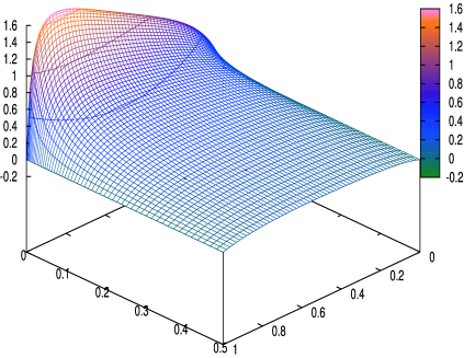
Refer to caption
(a)
Refer to caption
(b)
Refer to caption
(c)
Refer to caption
(d)
Figure 1: Unbounded variation case (σ=0.5𝜎0.5\sigma=0.5): computing the density of the overshoot f1(x,y)subscript𝑓1𝑥𝑦f_{1}(x,y) (x(0,1)𝑥01x\in(0,1), y(0,0.5)𝑦00.5y\in(0,0.5)), probability of first exit f2(x)subscript𝑓2𝑥f_{2}(x) and probability of creeping f3(x)subscript𝑓3𝑥f_{3}(x) for parameter Set 1 (positive drift μ=1𝜇1\mu=1) and Set 2 (negative drift μ=1𝜇1\mu=-1).
Refer to caption
(a)
Refer to caption
(b)
Refer to caption
(c)
Refer to caption
(d)
Figure 2: Bounded variation case (σ=0𝜎0\sigma=0): computing the density of the overshoot f1(x,y)subscript𝑓1𝑥𝑦f_{1}(x,y) (x(0,1)𝑥01x\in(0,1), y(0,0.5)𝑦00.5y\in(0,0.5)), probability of first exit f2(x)subscript𝑓2𝑥f_{2}(x) and probability of creeping f3(x)subscript𝑓3𝑥f_{3}(x) for parameter Set 3 (positive drift μ=1𝜇1\mu=1) and Set 4 (negative drift μ=1𝜇1\mu=-1).
Refer to caption
(a)
Refer to caption
(b)
Refer to caption
(c)
Refer to caption
(d)
Figure 3: Computing the density of the renewal measure 𝒰(ds,dx)𝒰d𝑠d𝑥{\mathcal{U}}({\textnormal{d}}s,{\textnormal{d}}x), s(0,0.25)𝑠00.25s\in(0,0.25) and x(0,0.5)𝑥00.5x\in(0,0.5).