Optimal control of non-Markovian open quantum systems via feedback

Abstract

The problem of optimal control of non-Markovian open quantum system via weak measurement is presented. Based on the non-Markovian master equation, we evaluate exactly the non-Markovian effect on the dynamics of the system of interest interacting with a dissipative reservoir. We find that the non-Markovian reservoir has dual effects on the system: dissipation and backaction. The dissipation exhausts the coherence of the quantum system, whereas the backaction revives it. Moreover, we design the control Hamiltonian with the control laws attained by the stochastic optimal control and the corresponding optimal principle. At last, we considered the exact decoherence dynamics of a qubit in a dissipative reservoir composed of harmonic oscillators, and demonstrated the effectiveness of our optimal control strategy. Simulation results showed that the coherence will completely lost in the absence of control neither in non-Markovian nor Markovian system. However, the optimal feedback control steers it to a stationary stochastic process which fluctuates around the target. In this case the decoherence can be controlled effectively, which indicates that the engineered artificial reservoirs with optimal feedback control may be designed to protect the quantum coherence in quantum information and quantum computation.

1 Introduction

Quantum information science has emerged as one of the most exciting scientific developments of the past decade. The most difficult problem in realizing the quantum information technology is that the quantum system can never be isolated from the surrounding environment completely. Interactions with the environment deteriorate the purity of quantum states. This general phenomenon, known as decoherence [1, 2], is a serious obstacle against the preservation of quantum superpositions over long periods of time. Decoherence entails nonunitary evolutions, with serious consequences, like a loss of information and probable leakage toward the environment. Thus, on the one hand, the information carried by a quantum system has to be protected from decoherence. On the other hand, a detailed knowledge of quantum dynamics and control will help to construct high precision devices that accurately perform their intended tasks despite large disturbances from the environment.

For the purpose of efficiently processing quantum information, results and methods coming from the classical control theory have been systematically introduced to manipulate practical quantum systems [3, 4, 5, 6, 7, 8, 9, 10, 11, 12, 13]. Early works aim to answer the questions like controllability and observability in finite dimensional closed quantum systems [14, 15]. They have many applications like molecular dynamics in quantum chemistry. As we demonstrated above, quantum systems are very vulnerable when exposed in a noisy environment. So, open quantum systems control is becoming a matter of concern for more and more physicists and cyberneticists. Recently, quantum control works include: (i) steering a quantum system from its initial state to a given final state or a set of final states [16]. Transferring to specific final states are very important for applications to quantum computing, quantum chemistry and atomic physics. (ii) Quantum decoherence control [3, 11]. Suppression of decoherence is essential to effectively protect quantum purity and quantum coherence. (iii) Quantum entanglement control [17, 18]. Reliable generation and distribution of entanglement in a quantum network is a central subject in quantum information technology, especially in quantum communication.

To the quantum control strategies, a number of interesting schemes have been proposed during the last few years in order to protect the purity and counter the effects of decoherence. It is just like the classical control theory, according to the principle of controllers’ design, the open quantum systems control includes open-loop control and closed-loop control. Quantum open-loop control means to design the controller without measurement. Early proposed quantum error-correction codes, error-avoiding codes and Bang-Bang control can be classified as open-loop control. Nowadays, by tuning the system’s Hamiltonian, coherent control theory has opened new perspective on decoherence and entanglement control. It can decouple a part of the system dynamics from decoherence, on which noiseless quantum information can be encoded either in Markovian open quantum systems or in non-Markovian open quantum system [19, 20]. The quantum coherent control plays an important role in state generation and transfer in quantum information, quantum chemistry and optical physical, and it is a focus these days. Feedback is the essential concept of classical control theory, but the study of feedback control has only a toehold in quantum control theory for many fundamental problems needed to be solved. The main problem is quantum measurement. Feedback control needs measurement to reduce the system’s uncertainty, whereas measuring a quantum system will inevitably lead to quantum state collapse, which increase the system’s uncertainty in turn [21]. As we demonstrated above, the theory of quantum measurement is strange in that it does not allow the noncommuting observables to be measured simultaneously. The essence of feedback control is expected to attain robustness to noise or modeling error, and quantum control using continuous measurement, so-called measurement based quantum feedback control, was proposed in early 90’s. Recently, the stochastic control theory has been exploited to the open quantum system. The theory of quantum feedback control with continuous measurement can be developed simply by replacing each ingredient of stochastic control theory by its noncommutative counterpart. The system and observations are described by quantum stochastic differential equations. The field of quantum stochastic control was pioneered by V. P. Belavkin in the remarkable paper [22] in which the quantum counterparts of nonlinear filtering and LQG control were developed. The advantage of the quantum stochastic approach is that the details of quantum probability and measurement are hidden in a quantum filtering equation. In view of physicists, they also reformulated the evolution of damped systems with output in the form of an explicitly stochastic evolution equation, which specifies the quantum trajectory of the systems. Feedback control of quantum mechanical systems which take into account the probabilistic nature of quantum measurement is one of the central problem in the control of such systems in both physics and control theory. Recently, superconducting qubits [23, 24] have also been studied as ways to control and interact with naturally formed quantum two-level systems in superconducting circuits. The two-level systems naturally occurring in Josephson junctions constitute a major obstacle for the operation of superconducting phase qubits. Since these two-level systems can possess remarkably long decoherence times, References [25, 26, 27] showed that such two-level systems can themselves be used as qubits, allowing for a well controlled initialization, universal sets of quantum gates, and readout. Thus, a single current-biased Josephson junction can be considered as a multi-qubit register. It can be coupled to other junctions to allow the application of quantum gates to an arbitrary pair of qubits in the system. These results [25, 26, 27] indicate an alternative way to control qubits coupled to naturally formed quantum two-level systems, for improved superconducting quantum information processing. Indeed, these predictions have been found experimentally in [28]. More recently, reference [29] applies quantum control techniques to control a large spin chain by only acting on two qubits at one of its ends, thereby implementing universal quantum computation by a combination of quantum gates on the latter and swap operations across the chain. They [29] show that the control sequences can be computed and implemented efficiently. Moreover, they discuss the application of these ideas to physical systems such as superconducting qubits in which full control of long chains is challenging.

The rest of the paper is organized as follows. In Section II, we introduce the open quantum system and the non-Markovian quantum master equation, and present the main difference between the non-Markovian quantum system and the Markovian one. The optimal control problem via quantum measurement feedback is precisely formulated in Section III. In Section IV, we specifically investigated the stochastic optimal control of Spin-Boson system. A useful numerical example is demonstrated in Section V, and a few concluding remarks are given in Section VI.

2 Open quantum system and non-Markovian master equation

The theory of open quantum system describes the dynamics of a system of interest interacting with its surrounding environment [1], and the quantum master equation governs the evolution of the quantum system, which plays an important role in relaxation and decoherence theory. Markovian approximation is usually used in this master equation under the assumption that the correlation time between the systems and environments is infinitely short. However, in some cases an exactly analytic description of the open quantum system dynamic is needed. Especially in high-speed communication the characteristic time scales become comparable with the reservoir correlation time, and in solid state devices memory effects are typically non negligible. So it is necessary to extensively study the non-Markovian case. In this paper, we will consider the optimal control of non-Markovian open quantum system via feedback, typically the quantum decoherence optimal control.

2.1 Open quantum system

Consider a quantum system $S$ embedded in a dissipative environment $B$ and interacting with a time-dependent external field, i.e., the control field. The total Hamiltonian has the general form

$$\begin{array}[]{rcl}\hat{H}_{tot}&=&\hat{H}_{S}+\hat{H}_{B}+\hat{H}_{I}\\ &=&\hat{H}_{0}+\hat{H}_{C}(t)+\hat{H}_{B}+\hat{H}_{I},\end{array}$$ (1)

where $\hat{H}_{0}$ is the system free Hamiltonian, $\hat{H}_{C}(t)$ the Hamiltonian of the control field (either open-loop or closed-loop), and $\hat{H}_{B}$ the bath and $\hat{H}_{I}$ the interaction between the free system and the bath. Note that the interaction between the control field and the free system or the bath are always negligible. The operator $\hat{H}_{C}(t)$ contains a time-dependent external field to adjust the quantum evolution of the system. One of the central goals of the theoretical treatment is then the analysis of the dynamical behavior of the populations and coherences, which are given by the elements of the reduced density matrix, defined as

$$\rho_{S}(t)=\tr_{B}[\rho_{tot}(t)],$$ (2)

where $\rho_{tot}$ is the total density matrix for both the system and the environment. For simplicity, it is always assumed as the system of a single atom which configured such that a transition between only two states is possible. The Hamiltonian of the environment is assumed to be composed of harmonic oscillators with natural frequencies $\omega_{i}$ and masses $m_{i}$,

$$\hat{H}_{B}=\sum_{i=1}^{N}\left(\frac{p_{i}^{2}}{2m_{i}}+\frac{m_{i}}{2}x_{i}^{2}\omega_{i}^{2}\right),$$ (3)

where $(x_{1},x_{2},\cdots,x_{N},p_{1},p_{2},\cdots,p_{N})$ are the coordinates and their conjugate momenta, and the Planck constant $\hbar=1$ in atomic units and the initial state of the system is $\rho(0)=\rho_{0}$ (for simplicity we write $\rho$ as $\rho_{S}$). For convenience, we always assume that the evolution starts from $t_{0}=0$. The interaction Hamiltonian between the system $S$ and the environment $B$ is assumed to be bilinear,

$$\hat{H}_{int}=\alpha\sum_{n}A_{n}\otimes B_{n}.$$ (4)

The interaction Hamiltonian in the interaction picture therefore takes the form

$$\begin{array}[]{rcl}\hat{H}_{int}(t)&=&e^{i(H_{S}+H_{B})t}H_{int}e^{-i(H_{S}+H_{B})t}\\ &=&\alpha\sum_{n}A_{n}(t)\otimes B_{n}(t),\end{array}$$ (5)

where

$$\begin{array}[]{rcl}A_{n}(t)&=&e^{iH_{S}t}A_{n}e^{-iH_{S}t},\\ B_{n}(t)&=&e^{iH_{B}t}B_{n}e^{-iH_{B}t}.\end{array}$$

The effect of the environment on the dynamics of the system can be seen as a interplay between the dissipation and fluctuation phenomena. And it is the general environment that makes the quantum system lose coherence (decoherence). The system-environment interaction leads to non-unitary reduced system dynamics.

2.2 Quantum master equations

The analysis of the time evolution of open quantum system plays an important role in many applications of modern physics. With the Born-Markovian approximation the dynamics is governed by a master equation of the relatively simple form

$$\frac{d}{dt}\rho(t)=-i[\hat{H}_{S}(t),\rho(t)]+\sum_{m}\gamma_{m}\mathcal{D}[C_{m}]\rho(t),$$ (6)

with a time-independent generator in the Lindblad form, her the superoperator $\mathcal{D}[L]\rho=L\rho L^{{\dagger}}-\frac{1}{2}L^{{\dagger}}L\rho-\frac{1}{2}\rho L^{{\dagger}}L$. This is the most general form for the generator of a quantum dynamical semigroup. The Hamiltonian $\hat{H}_{S}(t)$ describes the coherent part of the time evolution. Non-negative quantities $\gamma_{m}$ play the role of relaxation rates for the different decay modes of the open system. The operators $C_{m}$ are usually referred to as Lindblad operators which represent the various decay modes, and the corresponding density matrix equation (6) is called the Lindblad master equation. The solution of Eq. (6) can be written in terms of a linear map $V(t)=\exp(\mathcal{L}t)$ that transforms the initial state $\rho(0)$ into the state $\rho(t)=V(t)\rho(0)$ at time $t$. The physical interpretation of this map $V(t)$ requires that it preserves the trace and the positivity of the density matrix $\rho(t)$.

The most important physical assumption which underlies the Eq. (6) is the validity of the Markovian approximation of short environmental correlation times [17]. With this approximation, the environment acts as a sink for the system information. Due to the system-reservoir interaction, the system of interest loses information on its state into the environment, and this lost information does not play any further role in the system dynamics. However, if the environment has a non-trivial structure, then the seemingly lost information can return to the system at a later time leading to non-Markovian dynamics with memory. This memory effect is the essence of non-Markovian dynamics [31, 32, 33], which is characterized by pronounced memory effects, finite revival times and non-exponential relaxation and decoherence. Non-Markovian dynamics plays an important role in many fields of physics, such as quantum optics, quantum information, quantum chemistry process, especially in solid state physics. As a consequence the theoretical treatment of non-Markovian quantum dynamics is extremely demanding. However, in order to take into account quantum memory effect, an integro-differential equation is needed which has complex mathematical structure, thus prevent generally to solve the dynamics of the system of interest. An appropriate scheme is the time-covolutionless (TCL) projection operator technique which leads to a time-local first order differential equation for the density matrix.

The general structure of the TCL master equation is given by

$$\frac{d}{dt}\rho(t)=-i[\hat{H}_{S}(t),\rho(t)]+\sum_{m}\Delta_{m}(t)\mathcal{D}[C_{m}(t)]\rho(t).$$ (7)

The first term describes the unitary part of the evolution. The latter involves a summation over the various decay channels labeled by $m$ with corresponding time-dependent decay rates $\Delta_{m}(t)$ and arbitrary time-dependent system operators $C_{m}(t)$.

In the simplest case the rates $\Delta_{m}$ as well as the Hamiltonian $\hat{H}_{S}$ and the operators $C_{m}$ are assumed to be time-independent, that is, it is the Markovian case. Note that, for arbitrary time-dependent operators $\hat{H}_{S}(t)$ and $C_{m}(t)$, and for $\Delta_{m}(t)\geq 0$ the generator of the master equation (7) is still in Lindblad form for each fixed time $t$, which may be considered as time-dependent quantum Markovian process. However, if one or several of the $\Delta_{m}(t)$ become temporarily negative which expresses the presence of strong memory effects in the reduced system dynamics, the process is then said to be non-Markovian.

2.3 Quantum feedback control

Quantum feedback control was formally initiated by Belavkin’s work [15], [22] and so on. The main problem of optimal quantum feedback control is separated into quantum filtering which provides optimal estimates of the stochastic quantum operators and then an optimal control problem based on the output of the quantum measurement. As we demonstrated in the introduction, the quantum system is not directly observable. Since the very beginning of the quantum mechanics, the measurement process has been a most fundamental issue. The main characteristic feature of the quantum measurement is that the measurement changes the dynamical evolution. This is the main difference of the quantum measurement compared to its classical analogue. When one observes incompatible quantum events (self-adjoint orthoprojectors with $P^{2}=P=P^{*}$ ($*$ denotes the Hermitian adjoint) acting in some Hilbert space $\mathcal{H}$), the state of the system needs to be updated to account for the change to the system or back-action. This state change was traditionally described by the normalized projection postulate

$$\rho\rightarrow\rho_{i}=\frac{P_{i}\rho P_{i}}{\tr[\rho P_{i}]},$$

which also ensures instantaneous repeatability of the observed event corresponding to the projection $P_{i}$.

We now couple the system to a control field. If we assume no scattering between the measurement and control fields and assume a weak coupling such that information is not lost into the control field, then this effectively replaces the Hamiltonian $\hat{H}_{S}(t)$ of the system with a controlled Hamiltonian $\hat{H}_{0}(t)+\hat{H}(u(t))$ for admissible real valued control functions $u(t)\in\mathbb{R}$. The term feedback refers to control law $u(t)$, which is also a function of the state $\rho$. This control Hamiltonian generates the controlled unitaries $U_{t}(u(t))$ given the controlled flow $U_{t}^{*}(u_{t_{0}}^{T})\rho U_{t}(u_{t_{o}}^{T})$, where $u_{t_{0}}^{T}\equiv\{u(t)|t_{0}\leq t<T\}$ is the control process over the interval $[0,T)$. In classical control, we can allow complete observability of the controllable system, so that feedback controls are determined by the system variables. However, in quantum system the measurement are weak measurement (for non-observability of the system operators). So, the feedback controls should be given by a function of the stochastic output process $W_{F_{i}}(t)$, and measurement trajectory is fed into the controls $W_{F_{i}}(t)\rightarrow u_{t}(W_{F_{i}}(t))$.

Considering both controls on the systems and simultaneous quantum weak measurements over multiple observable $\{F_{i}\}$, we have following stochastic master equation and measurement outputs for the quantum feedback control system:

$$d\rho = -i[H_{0},\rho]dt+\sum_{k=1}^{r}u_{k}(t)(-i[H_{k},\rho])dt+\sum_{m}\Delta_{m}(t)\mathcal{D}[C_{m}]\rho dt$$ (8)

$$+\sum_{i}M_{i}\mathcal{D}[F_{i}]\rho dt+\sum_{i}\sqrt{M_{i}\eta_{i}}\mathcal{H}[F_{i}]\rho dW_{F_{i}}$$

$$dW_{F_{i}} = dY_{i}-\sqrt{\eta_{i}M_{i}}\tr\{F_{i}\rho\}dt$$ (9)

where $H_{k},~{}~{}k=1,2,\cdots,r$ are the control Hamiltonians adjusted by the time-dependent control laws $u_{k}(t)\in\mathbb{R}$ and the superoperator $\mathcal{H}[A]\rho=A\rho+\rho A-[\tr(A\rho+\rho A)]\rho$. Note that, the last two terms in Eq. (8) come from the measurement-induced disturbance (we will explain the degenerate in the next section from the quantum measurement view of point), where $M_{i}$ are the effective interaction strengths and $\eta_{i}$ are the detection efficiency coefficients. $Y_{i}$ are the observation process. In fact, the innovation process $W_{F_{i}}$ is a Wiener process, which satisfy following rules. The expectation of any integral over $dW_{F_{i}}$ or $dW_{F_{i}}^{*}$ vanishes. The differentials $dW_{F_{i}}$ , $dW_{F_{i}}^{*}$ commute with any adapted process. Finally, the quantum Itô rules are

$$dW_{F_{i}}dW_{F_{j}}^{*}=\delta_{F_{i},F_{j}}dt,~{}~{}dW_{F_{i}}^{2}=(dW_{F_{i}}^{*})^{2}=dW_{F_{i}}^{*}dW_{F_{i}}=0.$$

3 Stochastic optimal control of Spin-Boson system

We have described the quantum feedback controls and have obtained controlled master equations, the remaining question is: how do we choose the control strategy $u(t)$ to achieve a particular control goal? For a fixed function $u(t)$ the expression (8) becomes a stochastic differential equation and its solution $\rho^{*}(t)$ is called a trajectory of the quantum system relevant to the quantum control $u(t)$. In general, any trajectory $\rho^{*}(t)$ should fulfill some initial conditions. In this section we approach this problem using optimal control theory, where the control goal is expressed as the desire to minimize a certain cost functional $J(t,u,\rho)$.

The optimality of control is judged by the expected cost associated to the admissible control process $u_{t_{0}}^{T}$ for the finite duration $T$ of the experiment. Admissible control strategies are defined as those $u_{t_{0}}^{T}$ for which the operator valued cost integral

$$J[u(\cdot)]=\int_{t_{0}}^{T}L(\tau,u,\rho)d\tau+\theta\cdot g(\rho_{T},\rho^{*}),$$ (10)

and the solutions of Eq. (8) exist. Here $L$ is a function of time $t$, the current control law $u$, and the quantum state $\rho$. The function $g$, known as a target or bequest function in control theory, is a function of the state parameters at termination. We assume that both are continuous in their arguments. $\theta$ is the constant parameters to adjust the penalty functional between the two functions. The cost $J$ will vary from one experimental trial to another, and must be thought of as a random variable depending on the measurement output.

Here we consider a situation in which a single qubit interacts with a heat bath of bosons. We will make use of the two-level non-Markovian master equation. The kinetic equation of two-level strong coupling non-Markovian quantum system is the particular form of the Eq. (7) and (8), which performed a rotating wave approximation after tracing over the environment without neglecting the counter-rotating terms. By tracing out the bath degrees of freedom, we find for $\rho$ the feedback controlled two-level quantum system non-Markovian evolution equation

$$d\rho = -\frac{i}{2}\omega_{0}[\sigma_{z},\rho]dt-\frac{i}{2}u_{x}(t)[\sigma_{x},\rho]dt-\frac{i}{2}u_{y}(t)[\sigma_{y},\rho]dt$$ (11)

$$+ \Gamma_{1}(t)\mathcal{D}[\sigma^{-}]\rho dt+\Gamma_{2}(t)\mathcal{D}[\sigma^{+}]\rho dt+M\mathcal{D}\left[-\frac{\sigma_{z}}{2}\right]\rho dt$$

$$+ \sqrt{\eta M}\mathcal{H}\left[-\frac{\sigma_{z}}{2}\right]\rho dW\equiv f(t)$$

The free Hamiltonian of the one-qubit quantum system can be written as $H_{0}=\frac{\omega_{0}}{2}(|0\rangle\langle 0|-|1\rangle\langle 1|)=\frac{\omega_{0}}{2}\sigma_{z}$, where $|0\rangle$ and $|1\rangle$ are Dirac notations of its two eigenstates and $\omega_{0}$ is the Rabi frequency. $\sigma^{+}=\frac{1}{2}(\sigma_{x}+i\sigma_{y}),~{}~{}\sigma^{-}=\frac{1}{2}(\sigma_{x}-i\sigma_{y})$, with $\sigma_{x}$, $\sigma_{y}$, $\sigma_{z}$ the Pauli matrices. Here, the controlled part has two channels $H_{C}(t)=\frac{1}{2}u_{x}(t)\sigma_{x}+\frac{1}{2}u_{y}(t)\sigma_{y}$. The effective interaction strengths between the measurement and the system is $M\geq 0$.

Suppose $\rho=\frac{1}{2}\left(\begin{array}[]{cc}1+z&x-iy\\ x+iy&1-z\end{array}\right)$, thus corresponding to (11), we have the following evolution equations,

$$dx = \left(-\Delta(t)x-\frac{M}{2}x-\omega_{0}y+u_{y}(t)z\right)dt+\sqrt{M\eta}xzdW$$

$$dy = \left(\omega_{0}x-\Delta(t)y-\frac{M}{2}y-u_{x}(t)z\right)dt+\sqrt{M\eta}yzdW$$

$$dz = 2\left(-\frac{u_{y}(t)}{2}x+\frac{u_{x}(t)}{2}y-\Delta(t)z-\gamma(t)\right)dt$$ (12)

$$+\sqrt{M\eta}(-1+z^{2})dW.$$

Thus the coherence factor $\Lambda(t)=\sqrt{x^{2}+y^{2}}/2$, and the population $\rho_{00}(t)=(1+z)/2,~{}\rho_{11}(t)=(1-z)/2$.

Here, the objective is to compute an appropriate feedback control functions $u_{x}(t),~{}~{}u_{y}(t)$ steering the system from the initial state $\rho_{0}$ into a target state $\rho_{T}$ at final time $T$. The relative simple cost functional may be written as

$$J[u(t)]=\frac{\theta}{2}\|\rho(T)-\rho_{T}\|^{2}+\frac{1}{2}\int_{t_{0}}^{T}(u_{x}^{2}(t)+u_{y}^{2}(t))dt,$$ (13)

where $\|\cdot\|$ is the Frobenius norm: $\|A\|^{2}=\tr A^{{\dagger}}A=\sum_{ij}|A_{ij}|^{2}$. Here, the first term represents the deviation between the state of the system at final time $\rho(T)$ and the target state $\rho_{T}$, the second integral term penalizes the control field with $\theta>0$, the weighting factor used to achieve a balance between the tracking precision and the control constraints. Minimizing the first term is equivalent to maximizing the state transfer fidelity $F=\tr\{\rho(T)\rho_{T}\}$. Our overall task is to find control $u_{x}(t),~{}~{}u_{y}(t)$ that minimizes $J[u(t)]$ and satisfies both dynamic constraint and boundary condition. The optimal solution of this problem will be obtained using the optimal principle. The corresponding Hamiltonian function may be present in the form

$$\mathcal{H}(\rho,u,\lambda)=\mathbb{E}\left\{\frac{1}{2\theta}(u_{x}^{2}+u_{y}^{2})+\lambda^{T}(t)f(t)\right\},$$ (14)

where the adjoint state variable $\lambda(t)=[\lambda_{1}(t),\lambda_{2}(t),\lambda_{3}(t)]^{T}$ is the Lagrange multipliers introduced to implement the constraint. The optimal solution can be solved by the following differential equation with two-sided boundary values:

$$\dot{\rho} = \frac{\partial\mathcal{H}}{\partial\lambda},~{}~{}~{}~{}~{}~{}\rho(t_{0})=\rho_{0};$$ (15)

$$\dot{\lambda} = -\frac{\partial\mathcal{H}}{\partial\rho},~{}~{}~{}~{}~{}~{}\lambda(T)=\rho(T)-\rho_{T}.$$ (16)

Together with

$$\left.\frac{\partial\mathcal{H}}{\partial u}\right|_{*} = \frac{\partial\mathcal{H}(\rho^{*}(t),u^{*}(t),\lambda(t),t)}{\partial u}=0;$$ (17)

$$\left.\frac{\partial^{2}\mathcal{H}}{\partial u^{2}}\right|_{*} = \frac{\partial^{2}\mathcal{H}(\rho^{*}(t),u^{*}(t),\lambda(t),t)}{\partial u^{2}}\leq 0.$$ (18)

Take this into Eq.(3), we get the optimal control for the Spin-Boson system with Hamiltonian function Eq.(14)

$$u_{x}(t) = \frac{\theta}{2}\left\{\lambda_{2}(t)x_{3}(t)-\lambda_{3}(t)x_{2}(t)\right\},$$ (19)

$$u_{y}(t) = \frac{\theta}{2}\left\{\lambda_{3}(t)x_{1}(t)-\lambda_{1}(t)x_{3}(t)\right\}.$$ (20)

The influence of environmental disturbances include both relaxation and dephasing effects, which are formulated as $\Gamma_{1}(t)\mathcal{D}[\sigma^{-}]\rho$ and $\Gamma_{2}(t)\mathcal{D}[\sigma^{+}]\rho$. The time dependent coefficients $\Gamma_{1}(t)=\Delta(t)+\gamma(t)$ and $\Gamma_{2}(t)=\Delta(t)-\gamma(t)$, with $\Delta(t)$ and $\gamma(t)$ being the diffusive term and damping term respectively, which can be written up to the second order in the system-reservoir coupling constant, as follows,

$$\Delta(t)=\int_{0}^{t}d\tau k(\tau)\cos(\omega_{0}\tau),$$

$$\gamma(t)=\int_{0}^{t}d\tau\mu(\tau)\sin(\omega_{0}\tau),$$ (21)

with

$$k(\tau)=2\int_{0}^{\infty}d\omega J(\omega)\coth[\hbar\omega/2k_{B}T]\cos(\omega\tau),$$

$$\mu(\tau)=2\int_{0}^{\infty}d\omega J(\omega)\sin(\omega\tau),$$ (22)

being the noise and the dissipation kernels, respectively. The properties of the Eq. (11) strongly depend on the behavior of the dissipation and the noise kernel which, in turn, is determined by the spectral density $J(\omega)$. In order to obtain true irreversible dynamics one introduces a continuous distribution of bath modes and replaces the spectral density by a smooth function of the frequency $\omega$ of the bath modes. In particular we will consider the Ohmic spectral density with a Lorentz-Drude cutoff function,

$$J(\omega)=\frac{2\gamma_{0}}{\pi}\omega\frac{\omega_{c}^{2}}{\omega_{c}^{2}+\omega^{2}},$$ (23)

where $\gamma_{0}$ is the frequency-independent damping constant and usually assumed to be $1$. $\omega_{c}$ is the high-frequency cutoff. The analytic expression for the coefficients $\gamma(t)$and $\Delta(t)$ are given in [11, 18].

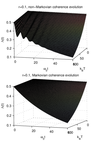
Figure 1: (Color online) Comparing the non-Markovian coherence dynamics with the Markovian one by the time evolution of $\Lambda(t)$ as a function of $k_{B}T$ for initial state $(x_{0},~{}y_{0},~{}z_{0})=\left(\frac{\sqrt{2}}{4},~{}\frac{\sqrt{2}}{4},~{}\frac{\sqrt{3}}{2}\right)$, $r=0.1$, $\omega_{0}=1$, and $\alpha^{2}=0.01$.

As we indicated above, temperature is the key factor in the non-Markovian system coefficients. In Fig. 1, we plot the coherence function $\Lambda(t)$ vs “temperature $k_{B}T$” vs $\omega_{0}t$ in $r=0.1$, and the initial state $(x_{0},~{}y_{0},~{}z_{0})=\left(\frac{\sqrt{2}}{4},~{}\frac{\sqrt{2}}{4},~{}\frac{\sqrt{3}}{2}\right)$ for the quantum system without control effect,

$$\frac{d}{dt}\rho(t)=-i[\hat{H}_{s}(t),\rho]+\Gamma_{1}(t)\mathcal{D}[\sigma^{-}]\rho+\Gamma_{2}(t)\mathcal{D}[\sigma^{+}]\rho.$$ (24)

From Fig. 1 we can compare the non-Markovian coherence dynamics with the Markovian one clearly. The up figure is the non-Markovian one from which we can see the oscillation of the $\Lambda(t)$. Moreover, at the low temperature especially $0$ temperature the non-Markovian effect is faint, as the temperature rises, the non-Markovian becomes more and more obvious, while the Markovian one decays exponentially. This phenomenon embodies the non-Markovian effect, which is evidently different from the Markovian property. The reason is that due to the non-Markovian memory effect, particularly $\Delta(t)<0$ in Eq (3), the coherence oscillates. With $\Delta(t)-\gamma(t)>0$ the quantum system coherence descended whilst $\Delta(t)-\gamma(t)<0$ the coherence ascended. In high temperature the Markovian quantum system decays exponentially and vanish only asymptotically, but in the non-Markovian system the coherence $\Lambda(t)$ oscillates, which is evidently different from the Markovian. In this case the non-Markovian property becomes evidently. From (3), we have learned that in the strong coupling, high temperature and high cutoff frequency regimes, the considerable back-action of the non- Markovian reservoir effectively counteracts the dissipation.

4 Example: quantum decoherence control

As is introduced in the introduction, quantum computing and quantum communication have attracted a lot of attention due to their promising applications such as the speedup of classical computations and secure key distributions. Although the physical implementation of basic quantum information processors has been reported recently, the realization of powerful and useable devices is still a challenging and yet unresolved task. A major difficulty arises from the coupling of a quantum system to its environment that leads to decoherence. Various methods have been proposed to reduce this unexpected effect in the past decade, which can be divided into coherent and incoherent control, according to how the controls enter the dynamics. However, the above control strategies render the quantum systems are always neglect the quantum measurement back-action or study simple systems with the Markovian approximation. In this paper, we restrict our discussion to the no-Markovian open quantum system, and consider its dynamics with feedback control and therefore the dynamics obeys the no-Markovian master equation (3).

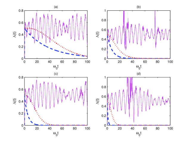
Figure 2: (Color online) Dynamics of coherence function $\Lambda(t)$ of non-Markovian optimal decoherence control (magenta solid line), non-Markovian without control (red dotted line), and Markovian without control (blue dashed line) for difference cases: (a) $r=0.5,~{}~{}k_{B}T=1$, (b)$r=3,~{}~{}k_{B}T=1$, (c)$r=0.5,~{}~{}k_{B}T=10$, and (d) $r=3,~{}~{}k_{B}T=10$ respectively. The other parameters are chosen as $M=0.05$, and $\eta=1$.

To quantify the decoherence dynamics of the qubit, we apply the following quantity $\Lambda(t)$ which is determined by the off-diagonal elements of the reduced density matrix.

$$\left|\rho_{12}(t)\right|=\Lambda(t)\left|\rho_{12}(0)\right|.$$ (25)

In the Bloch representation, we have

$$\Lambda(t)=\frac{\sqrt{x^{2}(t)+y^{2}(t)}}{\sqrt{x^{2}_{0}+y^{2}_{0}}}.$$ (26)

The decoherence factor maintains unity when the reservoir is absent and vanishes for the case of completely decoherence. For definiteness, we consider the following initial pure state of the qubit $|\psi(0)\rangle=\alpha|+\rangle+\beta|-\rangle.$ To use the optimal control method (15,16,19,20) we set the optimal control target $\rho_{T}$ as the free evolution $\dot{\rho_{T}}=-\frac{i}{2}[\omega_{0}\sigma_{z},\rho_{T}].$ It is easy to solve the equation with Bloch representation $x_{T}(t)=x_{0}\cos\omega_{0}t-y_{0}\sin\omega_{0}t,y_{T}(t)=x_{0}\sin\omega_{0}t+y_{0}\cos\omega_{0}t,z_{T}(t)=z_{0}.$

To demonstrate the effectiveness of our optimal control strategy, we present numerical simulations with the initial state $(x_{0},~{}y_{0},~{}z_{0})=\left(\frac{\sqrt{2}}{4},~{}\frac{\sqrt{2}}{4},~{}\frac{\sqrt{3}}{2}\right)$, and coupling constant $\alpha^{2}=0.01$, optimal control weighting factor $\theta=1$, and $\omega_{0}=1$ as the norm unit. Moreover, we regard the temperature as a key factor in decoherence process. Another reservoir parameter playing a key role in the dynamics of the system is the ratio $r=\omega_{c}/\omega_{0}$ between the reservoir cutoff frequency $\omega_{c}$ and the system oscillator frequency $\omega_{0}$. In Fig. 2, we plot the dynamics of coherence function $\Lambda(t)$ of non-Markovian optimal decoherence control (magenta solid line), non-Markovian without control (red dotted line), and Markovian without control (blue dashed line) for difference cases: (a) $r=0.5,~{}~{}k_{B}T=1$, (b)$r=3,~{}~{}k_{B}T=1$, (c)$r=0.5,~{}~{}k_{B}T=10$, and (d) $r=3,~{}~{}k_{B}T=10$ respectively. The other parameters are chosen as $M=0.05$, and $\eta=1$. From Fig. 2, it is worth noting that as increasing the ratio $r$, or increasing the temperature $k_{B}T$ the coherence lasting time becomes shorter and shorter. From Fig.1 we have known that non-Markovian reservoir has dual effects on the qubit: dissipation and back-action. The dissipation effect exhausts the coherence of the qubit, whereas the back-action one revives it. Here we still can observe the dynamical mechanism of the non-Markovian effect: the non-Markovian system’s coherence lasting time is always longer than the Markovian one. From the simulation results, the coherence function $\Lambda(t)$ will be completely lost in the absence of control neither non-Markovian system (dotted line) nor Markovian system (dashed line). However, the feedback control steers it to a stationary stochastic process which fluctuates around the target.

5 Conclusions

In conclusion, we have investigated the problem of optimal control of non-Markovian open quantum system via feedback. At first we analyzed the non-Markovian quantum system and the master equation. In general, the reduction of the degrees of freedom in the effective description of the open system results in non-Markovian behavior. The non-Markovian master equation for the quantum system thus supports to investigation of non-Markovian effects beyond the Born-Markovian approximation. In this paper we make a thorough examination of the difference between the Markovian system and the non-Markovian one. The main difference is that in the non-Markovian master equation, one or several of the dissipation coefficients become temporarily negative which expresses the presence of strong memory effects in the reduced system dynamics. From our analytic and numerical results, we find that the non-Markovian reservoir has dual effects on the qubit: dissipation and backaction. The dissipation effect exhausts the coherence of the qubit, whereas the backaction one revives it. In the strong coupling, high temperature and high cutoff frequency regimes, the considerable backaction of the non-Markovian reservoir effectively counteracts the dissipation.

Based on the non-Markovian master equation we analyzed the optimal control problem via feedback. For the quantum system is typically different to the classical one, the quantum measurement changes the dynamical evolution. Hence, we consider the quantum weak measurement and the corresponding master equation is the stochastic one. Moreover, we designed the control Hamiltonian with the control laws attained by the stochastic optimal control problem and the corresponding optimal principle. Usually this kind of problem is difficult to be analytically solved. We considered this problem in the non-Markovian two-level system. Through transforming its master equation into the Bloch vector representation we obtained the corresponding differential equation with two-sided boundary values.

At last, we considered the exact decoherence dynamics of a qubit in a dissipative reservoir composed of harmonic oscillators, and demonstrated the effectiveness of our optimal control strategy. Obviously, the coherence function will be completely lost in the absence of control neither non-Markovian system nor Markovian system. However, the feedback control steers it to a stationary stochastic process which fluctuates around the target. In this case the decoherence can be controlled effectively, which may indicates that the decoherence rate can be slowed down and decoherence time can be delayed through design engineered reservoirs.

References

References

- [1] Breuer H P and Petruccione F 2002 The Theory of Open Quantum Systems (Oxford: Oxford University Press)
- [2] Weiss U 1999 Quantum Dissipative Systems (Second Edition) (Singapore: World Scientific Publishing)
- [3] Zhang J, Li C W, Wu R B, Tarn T J, and Liu X S 2005 J. Phys. A: Math. Gen. 38 6587
- [4] Zhang J, Wu R B, Li C W and Tarn T J 2009 J. Phys. A: Math. Theor. 42 035304
- [5] Zhang J, Wu R B, Li C W, Tarn T J and Wu J W 2007 Phys. Rev. A, 75 022324
- [6] Wiseman H M and Milburn G J 1993 Phys. Rev. Lett. 70 548
- [7] Rabitz H, de Vivie-Riedle R, Motzkus M and Kompa K 2002 Science 288 824
- [8] Wiseman H M and Milburn G J 2010Quantum Measurement and Control (Cambridge: Cambridge University Press)
- [9] Wu R B, Tarn T J and Li C W 2006 Phys. Rev. A, 73 012719
- [10] Zhang M, Dai H Y, Zhu X C, Li X M and Hu D W 2006 Phys. Rev. A 73 032101
- [11] Cui W, Xi Z R and Pan Y 2008 Phys. Rev. A 77 032117
- [12] Pan Y, Xi Z R and Cui W 2010 Phys. Rev. A 81 022309
- [13] Xi Z and Jin G, 2008 Physical A: Statistical Mechanics and its Applications, 387 no.4, 1056
- [14] Tarn T J, Huang G M and Clark J W 1980 Mathematical Modeling 1 109
- [15] Belavkin V P 1983 Autom. Rem. Control 44 178
- [16] Wei L F, Johansson J R, Cen L X, Ashhab S and Nori F 2008 Phys. Rev. Lett. 100 113601
- [17] Cui W, Xi Z R and Pan Y 2009 J. Phys. A: Math. Theor. 42 025303
- [18] Cui W, Xi Z R and Pan Y 2009 J. Phys. A: Math. Theor. 42 155303
- [19] Maniscalco S, Olivares S and Paris M G A 2007 Phys Rev. A 75 062119
- [20] Maniscalco S, Piilo J, Intravaia F, Petruccione F and Messina A 2004 Phys. Rev. A 70 032113
- [21] Qi B 2009 Science in China Series F 52 2313
- [22] Belavkin V P 1992 J. Multivar. Anal 42 171
- [23] You J Q and Nori F 2005 Physics Today 58 No. 11 42
- [24] Liu Y X, You J Q, Wei L F, Sun C P and Nori F 2005 Phys. Rev. Lett. 95 087001
- [25] Zagoskin A M, Ashhab S, Johansson J R and Nori F 2006 Phys. Rev. Lett. 97 077001
- [26] Ashhab S, Johansson J.R. and Nori F 2006 Physica C 444 45
- [27] Ashhab S, Johansson J R and Nori F 2006 New J. Phys. 8 103
- [28] Neeley M et al. 2008 Nature Physics 4 523
- [29] Burgarth D, Maruyama K, Murphy M, Montangero S, Calarco T, F. Nori and Plenio M B arXiv:0905.3373
- [30] Burgarth D, Maruyama K and Nori F 2009 Phys. Rev. A 79 020305(R)
- [31] Wiseman H M and Gambetta J M 2008 Phys. Rev. Lett. 101 140401
- [32] Piilo J, Maniscalco S, Härkönen K and Suominen K A 2008 Phys. Rev. Lett. 100 180402
- [33] Wolf M M, Eisert J, Cubit T S and Cirac J I 2008 Phys. Rev. Lett. 101 150402