Structure of Defective Crystals at Finite Temperatures:
A Quasi-Harmonic Lattice Dynamics Approach

Abstract

In this paper we extend the classical method of lattice dynamics to defective crystals with partial symmetries. We start by a nominal defect configuration and first relax it statically. Having the static equilibrium configuration, we use a quasiharmonic lattice dynamics approach to approximate the free energy. Finally, the defect structure at a finite temperature is obtained by minimizing the approximate Helmholtz free energy. For higher temperatures we take the relaxed configuration at a lower temperature as the reference configuration. This method can be used to semi-analytically study the structure of defects at low but non-zero temperatures, where molecular dynamics cannot be used. As an example, we obtain the finite temperature structure of two $180^{\circ}$ domain walls in a 2-D lattice of interacting dipoles. We dynamically relax both the position and polarization vectors. In particular, we show that increasing temperature the domain wall thicknesses increase.

1 Introduction

Although it has been recognized that defects play an important role in nanostructured materials, the fundamental understanding of how defects alter the material properties is not satisfactory. The link between defects and the macroscopic behavior of materials remains a challenging problem. Classical mechanics of defects that studies materials with microscale defects is based on continuum theories with phenomenological constitutive relations. In the nanoscale, the continuum quantities such as stress and strain become ill defined. In addition, due to size effects, to study defects in nano-structured materials, non-classical solutions of defect fields is necessary [22]. The application of continuum mechanics to small-scale problems is problematic; atomistic numerical methods such as ab initio calculations [43, 48], Molecular Dynamics (MD) simulations [25, 21] and Monte Carlo (MC) simulations [70, 45] can be used for nanoscale mechanical analyses. However, the application of these methods is largely restricted by the size limit and the periodicity requirements. Current ab initio techniques are unable of handling systems with more than a few hundred atoms. Molecular dynamics simulations can model larger systems, however, MD is based on equations of classical mechanics and thus cannot be used for low temperatures, where quantum effects are dominant. Engineering with very small structures requires the ability to solve inverse problems and this cannot be achieved through purely numerical methods. What is ideally needed is a systematic method of analysis of solids with defects that is capable of treating finite temperature effects.

The only analytic/semi-analytic method for solving zero-temperature defect problems in the lattice scale is the method of lattice statics. The method of lattice statics was introduced in [41, 26]. This method has been used for point defects [14, 16], for cracks [10, 11, 24], and also for dislocations [4, 11, 12, 40, 55, 63]. More details and history can be found in [3, 4, 5, 14, 15, 20, 44, 49, 55, 64] and references therein. Lattice statics is based on energy minimization and cannot be used at finite temperatures. The other restriction of most lattice statics calculations is the harmonic approximation, which can be too crude close to defects. Recently, motivated by applications in ferroelectrics, we developed a general theory of anharmonic lattice statics capable of semi-analytic modeling of different defective crystals governed by different types of interatomic potentials [68, 69, 28]. At finite temperatures, the use of quantum mechanics-based lattice dynamics is necessary. Unfortunately, lattice dynamics has mostly been used for perfect crystals and for understanding their thermodynamic properties [3, 8, 32, 35, 44, 51, 65]. There is not much in the literature on corrections for anharmonic effects and systematic solution techniques for defective crystals. Some of these issues will be addressed in this paper.

In order to accurately predict the mechanical properties of nanosize devices one would need to take into account the effect of finite temperatures. It should be mentioned that most multiscale methods so far have been formulated for $T=0$ calculations. An example is the quasi-continuum method [49, 57]. However, recently there have been several attempts in extending this method for finite temperatures [7, 9, 36, 58]. As Forsblom, et al. [19] mention, very little is known about the vibrational properties of defects in crystalline solids. Sanati and Esetreicher [54] showed the importance of vibrational effects in semi-conductors and the necessity of free energy calculations. Lattice dynamics [3, 51] has been ignored with the exception of some very recent works [60]. As examples of finite-temperature defect solutions we can mention Taylor, et al. [59, 61] who discuss quasiharmonic lattice dynamics for three-body interactions in bulk crystals. Taylor, et al. [62] consider a slab, i.e., a system that is periodic only in two directions. They basically consider a supercell that is repeated in the plane periodically. As Allan, et al. [1, 2] conclude, a combination of quasiharmonic lattice dynamics, molecular dynamics, Monte Carlo simulations and ab initio calculations should be used in real applications. However, at this time there is no systematic method of lattice dynamics for thermodynamic analysis of defective systems that is also capable of capturing the anharmonic effects. We should mention that in many materials systems lattice dynamics is a valid approximation up to two-third of the bulk melting temperature but it turns out that harmonic approximation may not be adequate for free energy calculations of defects at high temperatures (see [18] for discussions on Cu). Hansen, et al. [23] show that for Al surfaces above the Debye temperature quasiharmonic lattice dynamic approximation starts to fail. Zhao, et al. [71] show that quasiharmonic lattice dynamics accurately predicts the thermodynamic properties of silicon for temperatures up to $800~{}K$. In this paper, we are interested in low temperatures where MD fails while quasi-harmonic lattice dynamics is a good approximation.

For understanding defect structures the main quantity of interest is the Helmholtz free energy. Free energy is an important thermodynamic function that determines the relative phase stability and can be used to generate other thermodynamic functions. In quasiharmonic lattice dynamics, for a system of $n$ atoms, free energy is computed by diagonalizing a $3n\times 3n$ matrix that is obtained by quadratizing the Hamiltonian about a given static equilibrium configuration. Using similar ideas, for a perfect crystal with a unit cell with $N$ atoms, one can compute the free energy by diagonalizing a $3N\times 3N$ matrix in the reciprocal space. In the local quasiharmonic approximation one assumes that atoms vibrate independently and thus all is needed for calculation of free energy is to diagonalize $n$ $3\times 3$ matrices [38] (see Rickman and LeSar [53] for a recent review of the existing methods for free energy calculations). These will be discussed in more detail in §3.

In this paper, we propose a theoretical framework of quasi-harmonic lattice dynamics to address the mechanics of defects in crystalline solids at low but finite temperatures. The main ideas are summarized as follows. We think of a defective lattice problem as a discrete deformation of a collection of atoms to a discrete current configuration. The lattice atoms are assumed to interact through some interatomic potentials. At finite temperatures, the equilibrium positions of the atoms are not the same as their static equilibrium ($T=0$) positions; the lattice atoms undergo thermal vibrations. The potential and Helmholtz free energies of the lattice are taken as discrete functionals of the discrete deformation mapping. For finite temperature equilibrium problems, the discrete nonlinear governing equations are linearized about a reference configuration. The finite-temperature equilibrium configuration of the defective lattice can then be obtained semi-analytically. For finite temperature dynamic problems, the Euler-Lagrange equations of motion of the lattice are casted into a system of ordinary differential equations by superimposing the phonon modes. We should emphasize that our method of lattice dynamics is not restricted to finite systems; defects in infinite lattices can be analyzed semi-analytically. The only restriction is the use of interatomic potentials.

This paper is structured as follows. In §2 we briefly review the theory of anharmonic lattice statics presented in [68] and [69]. We then present an overview of the basic ideas of the method of lattice dynamics for both finite and infinite atomic systems in §3. This follows by an extension of these ideas to defective crystals with partial symmetries. In §4 we formulate the lattice dynamics governing equations for a 2-D lattice of dipoles with both short and long-range interactions. In §5 we study the temperature dependence of the structure of two $180^{\circ}$ domain walls in the dipole lattice. Conclusions are given in §6.

2 Anharmonic Lattice Statics

Consider a collection of atoms $\mathcal{L}$ with the current configuration $\left\{\mathbf{x}^{i}\right\}_{i\in\mathcal{L}}\subset\mathbb{R}^{n}$. Assuming that there is a discrete field of body forces $\{\mathbf{F}^{i}\}_{i\in\mathcal{L}}$, a necessary condition for the current position $\{\mathbf{x}^{i}\}_{i\in\mathcal{L}}$ to be in static equilibrium is $-\frac{\partial\mathcal{E}}{\partial\mathbf{x}^{i}}+\mathbf{F}^{i}=\mathbf{0},~{}\forall~{}i\in\mathcal{L}$, where $\mathcal{E}$ is the total static energy and is a function of the atomic positions. These discrete governing equations are highly nonlinear. In order to obtain semi-analytical solutions, we first linearize the governing equations with respect to a reference configuration $\mathcal{B}_{0}=\{\mathbf{x}^{i}_{0}\}_{i\in\mathcal{L}}$ [68]. We leave the reference configuration unspecified; at this point it would be enough to know that we usually choose the reference configuration to be a nominal defect configuration [68, 69, 28].

Taylor expansion of the governing equations for an atom $i$ about the reference configuration $\mathcal{B}_{0}=\{\mathbf{x}^{i}_{0}\}_{i\in\mathcal{L}}$ reads

$$-\frac{\partial\mathcal{E}}{\partial\mathbf{x}^{i}}+\mathbf{F}^{i}=-\frac{\partial\mathcal{E}}{\partial\mathbf{x}^{i}}\left(\mathcal{B}_{0}\right)-\frac{\partial^{2}\mathcal{E}}{\partial\mathbf{x}^{i}\partial\mathbf{x}^{i}}\left(\mathcal{B}_{0}\right)\cdot(\mathbf{x}^{i}-\mathbf{x}^{i}_{0})-\sum_{\begin{subarray}{l}j\in\mathcal{L}\\ j\neq i\end{subarray}}\frac{\partial^{2}\mathcal{E}}{\partial\mathbf{x}^{j}\partial\mathbf{x}^{i}}\left(\mathcal{B}_{0}\right)\cdot(\mathbf{x}^{j}-\mathbf{x}^{j}_{0})-...+\mathbf{F}^{i}=\mathbf{0}.$$ (1)

Ignoring terms that are quadratic and higher in $\{\mathbf{x}^{j}-\mathbf{x}^{j}_{0}\}$, we obtain

$$\frac{\partial^{2}\mathcal{E}}{\partial\mathbf{x}^{i}\partial\mathbf{x}^{i}}\left(\mathcal{B}_{0}\right)\cdot(\mathbf{x}^{i}-\mathbf{x}^{i}_{0})+\sum_{\begin{subarray}{l}j\in\mathcal{L}\\ j\neq i\end{subarray}}\frac{\partial^{2}\mathcal{E}}{\partial\mathbf{x}^{j}\partial\mathbf{x}^{i}}\left(\mathcal{B}_{0}\right)\cdot(\mathbf{x}^{j}-\mathbf{x}^{j}_{0})=-\frac{\partial\mathcal{E}}{\partial\mathbf{x}^{i}}\left(\mathcal{B}_{0}\right)+\mathbf{F}^{i}~{}~{}~{}~{}~{}\forall i\in\mathcal{L}.$$ (2)

Here, $\left\{-\frac{\partial\mathcal{E}}{\partial\mathbf{x}^{i}}\left(\mathcal{B}_{0}\right)\right\}_{i\in\mathcal{L}}$ is the discrete field of unbalanced forces.

Defective Crystals and Symmetry Reduction.

In many defective crystals one can simplify the calculations by exploiting symmetries. A defect, by definition, is anything that breaks the translation invariance symmetry of the crystal. However, it may happen that a given defect does not affect the translation invariance of the crystal in one or two directions. With this idea, one can classify defective crystals into three groups: (i) with 1-D symmetry reduction, (ii) with 2-D symmetry reduction and (iii) with no symmetry reduction. Examples of (i), (ii) and (iii) are free surfaces, dislocations, and point defects, respectively [68]. Assume that the defective crystal $\mathcal{L}$ has a 1-D symmetry reduction, i.e. it can be partitioned into two-dimensional equivalence classes as follows

$$\mathcal{L}=\bigsqcup_{\alpha\in\mathbb{Z}}\bigsqcup_{I=1}^{N}\mathcal{S}_{I\alpha},$$ (3)

where $\mathcal{S}_{I\alpha}$ is the equivalence class of all the atoms of type $I$ and index $\alpha$ (see [68] and [28] for more details). Here, we assume that $\mathcal{L}$ is a multilattice of $N$ simple lattices. For a free surface, for example, each equivalence class is a set of atoms lying on a plane parallel to the free surface. Using this partitioning for $i=I\alpha$ one can write

$$\sum_{\begin{subarray}{l}j\in\mathcal{L}\\ j\neq i\end{subarray}}\frac{\partial^{2}\mathcal{E}}{\partial\mathbf{x}^{j}\partial\mathbf{x}^{i}}\left(\mathcal{B}_{0}\right)\cdot(\mathbf{x}^{j}-\mathbf{x}^{j}_{0})=\sideset{}{{}^{\prime}}{\sum}_{\beta\in\mathbb{Z}}\sum_{J=1}^{N}\sum_{j\in\mathcal{S}_{J\beta}}\frac{\partial^{2}\mathcal{E}}{\partial\mathbf{x}^{j}\partial\mathbf{x}^{i}}(\mathcal{B}_{0})\cdot\left(\mathbf{x}^{J\beta}-\mathbf{x}^{J\beta}_{0}\right),$$ (4)

where the prime on the first sum means that the term $J\beta=I\alpha$ is omitted. The linearized discrete governing equations are then written as [68]

$$\sideset{}{{}^{\prime}}{\sum}_{\beta\in\mathbb{Z}}\sum_{J=1}^{N}\mathbf{K}_{I\alpha J\beta}\mathbf{u}^{J\beta}+\left(-\sideset{}{{}^{\prime}}{\sum}_{\beta\in\mathbb{Z}}\sum_{J=1}^{N}\mathbf{K}_{I\alpha J\beta}\right)\mathbf{u}^{I\alpha}=\mathbf{f}_{I\alpha},$$ (5)

where

$$\mathbf{K}_{I\alpha J\beta}=\sum_{j\in\mathcal{S}_{J\beta}}\frac{\partial^{2}\mathcal{E}}{\partial\mathbf{x}^{j}\partial\mathbf{x}^{I\alpha}}(\mathcal{B}_{0}),~{}~{}\mathbf{f}_{I\alpha}=-\frac{\partial\mathcal{E}}{\partial\mathbf{x}^{I\alpha}}(\mathcal{B}_{0})+\mathbf{F}_{I\alpha},~{}~{}\mathbf{u}^{J\beta}=\mathbf{x}^{J\beta}-\mathbf{x}^{J\beta}_{0}=\mathbf{x}^{j}-\mathbf{x}^{j}_{0}~{}~{}~{}~{}~{}\forall~{}j\in\mathcal{S}_{J\beta}.$$ (6)

The governing equations in terms of unit cell displacement vector $\mathbf{U}_{\alpha}=\left(\mathbf{u}^{1}_{\alpha},...,\mathbf{u}^{N}_{\alpha}\right)^{\textsf{T}}$ can be written as

$$\sum_{\beta\in\mathbb{Z}}\mathbf{A}_{\beta}(\alpha)\mathbf{U}_{\alpha+\beta}=\mathbf{F}_{\alpha}~{}~{}~{}~{}~{}\alpha\in\mathbb{Z},$$ (7)

where $\mathbf{A}_{\beta}(\alpha)\in\mathbb{R}^{3N\times 3N},~{}\mathbf{U}_{\alpha},\mathbf{F}_{\alpha}\in\mathbb{R}^{3N}$. This is a linear vector-valued ordinary difference equation with variable coefficient matrices. The unit cell force vectors and the unit cell stiffness matrices are defined as

$$\mathbf{F}_{\alpha}=\left(\begin{array}[]{c}\mathbf{F}_{1\alpha}\\ \vdots\\ \mathbf{F}_{N\alpha}\\ \end{array}\right),~{}\mathbf{A}_{\beta}(\alpha)=\left(\begin{array}[]{cccc}\mathbf{K}_{1\alpha 1\beta}&\mathbf{K}_{1\alpha 2\beta}&\cdots&\mathbf{K}_{1\alpha N\beta}\\ \mathbf{K}_{2\alpha 1\beta}&\mathbf{K}_{2\alpha 2\beta}&\cdots&\mathbf{K}_{2\alpha N\beta}\\ \vdots&\vdots&\cdots&\vdots\\ \mathbf{K}_{N\alpha 1\beta}&\mathbf{K}_{N\alpha 2\beta}&\cdots&\mathbf{K}_{N\alpha N\beta}\\ \end{array}\right)~{}~{}~{}~{}~{}\alpha,\beta\in\mathbb{Z}.$$ (8)

Note that, in general, $\mathbf{A}_{\beta}$ need not be symmetric [68]. The resulting system of difference equations can be solved directly or using discrete Fourier transform [68].

Hessian Matrix for the Bulk Crystal.

A bulk crystal is a defective crystal with a $0$-D symmetry reduction. Governing equations for atom $I$ in the unit cell $\mathbf{n}=\mathbf{0}$ read $-\frac{\partial\mathcal{E}}{\partial\mathbf{x}^{I}}+\mathbf{F}_{I}=\mathbf{0},~{}I=1,...,N$. Linearization about $\mathcal{B}_{0}=\{\mathbf{X}^{I}\}$ yields

$$\frac{\partial^{2}\mathcal{E}}{\partial\mathbf{x}^{I}\partial\mathbf{x}^{I}}(\mathcal{B}_{0})\cdot(\mathbf{x}^{I}-\mathbf{X}^{I})+\sum_{\begin{subarray}{l}j\in\mathcal{L}\\ j\neq I\end{subarray}}\frac{\partial^{2}\mathcal{E}}{\partial\mathbf{x}^{I}\partial\mathbf{x}^{j}}(\mathcal{B}_{0})\cdot(\mathbf{x}^{j}-\mathbf{X}^{j})+...=-\frac{\partial\mathcal{E}}{\partial\mathbf{x}^{I}}(\mathcal{B}_{0})+\mathbf{F}_{I}~{}~{}~{}~{}~{}~{}~{}I=1,...,N.$$ (9)

Note that

$$\sum_{\begin{subarray}{l}j\in\mathcal{L}\\ j\neq I\end{subarray}}\frac{\partial^{2}\mathcal{E}}{\partial\mathbf{x}^{I}\partial\mathbf{x}^{j}}(\mathcal{B}_{0})\cdot(\mathbf{x}^{j}-\mathbf{X}^{j})=\sum_{\begin{subarray}{l}J=1\\ J\neq I\end{subarray}}^{N}\sum_{j\in\mathcal{L}_{J}}\frac{\partial^{2}\mathcal{E}}{\partial\mathbf{x}^{I}\partial\mathbf{x}^{j}}(\mathcal{B}_{0})\cdot(\mathbf{x}^{j}-\mathbf{X}^{j})+\sum_{\begin{subarray}{l}j\in\mathcal{L}_{I}\\ j\neq I\end{subarray}}\frac{\partial^{2}\mathcal{E}}{\partial\mathbf{x}^{I}\partial\mathbf{x}^{j}}(\mathcal{B}_{0})\cdot(\mathbf{x}^{j}-\mathbf{X}^{j}).$$ (10)

We also know that because of translation invariance of the potential

$$\frac{\partial^{2}\mathcal{E}}{\partial\mathbf{x}^{I}\partial\mathbf{x}^{I}}(\mathcal{B}_{0})=-\sum_{\begin{subarray}{l}j\in\mathcal{L}\\ j\neq I\end{subarray}}\frac{\partial^{2}\mathcal{E}}{\partial\mathbf{x}^{I}\partial\mathbf{x}^{j}}(\mathcal{B}_{0}).$$ (11)

Therefore, the linearized governing equations can be written as

$$\sum_{\begin{subarray}{l}J=1\\ J\neq I\end{subarray}}^{N}\mathbf{K}_{IJ}\mathbf{u}^{J}+\Bigg{(}\!\!-\sum_{\begin{subarray}{l}J=1\\ J\neq I\end{subarray}}^{N}\mathbf{K}_{IJ}\Bigg{)}\mathbf{u}^{I}=\mathbf{f}^{I}~{}~{}~{}~{}~{}~{}~{}~{}~{}I=1,...,N,$$ (12)

where

$$\mathbf{K}_{IJ}=\sum_{j\in\mathcal{L}_{J}}\frac{\partial^{2}\mathcal{E}}{\partial\mathbf{x}^{I}\partial\mathbf{x}^{j}}(\mathcal{B}_{0}),~{}~{}~{}\mathbf{f}^{I}=-\frac{\partial\mathcal{E}}{\partial\mathbf{x}^{I}}(\mathcal{B}_{0})+\mathbf{F}_{I},~{}~{}~{}\mathbf{u}^{J}=\mathbf{x}^{J}-\mathbf{X}^{J}=\mathbf{x}^{j}-\mathbf{X}^{j}~{}~{}~{}~{}~{}\forall~{}j\in\mathcal{L}_{J}.$$ (13)

The Hessian matrix of the bulk crystal is defined as

$$\mathbf{H}=\left(\begin{array}[]{cccc}\mathbf{K}_{11}&\mathbf{K}_{12}&\ldots&\mathbf{K}_{1N}\\ \mathbf{K}_{21}&\mathbf{K}_{22}&\ldots&\mathbf{K}_{2N}\\ \vdots&\vdots&\ddots&\vdots\\ \mathbf{K}_{N1}&\mathbf{K}_{N2}&\ldots&\mathbf{K}_{NN}\\ \end{array}\right),$$ (14)

where $\mathbf{K}_{JI}=\mathbf{K}_{IJ}$. Stability of the bulk crystal dictates $\mathbf{H}$ to be positive-semidefinite with three zero eigenvalues. In the case of a defective crystal, one can look at a sequence of sublattices containing the defect and calculate the corresponding sequence of Hessians.

3 Method of Quasi-Harmonic Lattice Dynamics

At a finite temperature $T$ (constant volume) thermodynamic stability is governed by Helmholtz free energy $F=E-TS$. In principle, $F$ is well-defined in the setting of statistical mechanics. Quantum-mechanically calculated energy levels $E(i)$ for different microscopic states can be used to obtain the partition function [33, 66]

$$Q=\sum_{i}\exp\left(\frac{-E(i)}{k_{B}T}\right),$$ (15)

where $k_{B}$ is Boltzman’s constant. Finally $F=-k_{B}T\ln Q$ (see the appendix). However, one should note that the phase space is astronomically large even for a finite system. Usually, in practical problems, molecular dynamics and Monte Carlo simulations, coupled with thermodynamic integration techniques, reduce the complexity of the free energy calculations. For low to moderately high temperatures, quantum treatment of lattice vibrations in the harmonic approximation provides a reliable description of thermodynamic properties [44]. In the following we review the classical formulation of lattice dynamics first for a finite collection of atoms and then for bulk crystals.

3.1 Finite Systems

For a finite system of $N$ atoms suppose $\mathcal{B}=\left\{\mathbf{X}^{i}\right\}_{i\in\mathcal{L}}$ is the static equilibrium configuration, i.e. $\frac{\partial\mathcal{E}}{\partial\mathbf{x}^{i}}\big{|}_{\mathbf{x}^{i}=\mathbf{X}^{i}}=\mathbf{0},~{}\forall~{}i\in\mathcal{L}$. Hamiltonian of this collection is written as

$$\mathcal{H}\left(\left\{\mathbf{x}^{i}\right\}_{i\in\mathcal{L}}\right)=\frac{1}{2}\sum_{i\in\mathcal{L}}m_{i}|\dot{\mathbf{x}}^{i}|^{2}+\mathcal{E}\left(\left\{\mathbf{x}^{i}\right\}_{i\in\mathcal{L}}\right).$$ (16)

Now denoting the thermal displacements by $\mathbf{u}^{i}=\mathbf{x}^{i}-\mathbf{X}^{i}$ potential energy of the system is written as

$$\mathcal{E}\left(\left\{\mathbf{x}^{i}\right\}_{i\in\mathcal{L}}\right)=\mathcal{E}\left(\left\{\mathbf{X}^{i}\right\}_{i\in\mathcal{L}}\right)+\frac{1}{2}\sum_{i,j\in\mathcal{L}}\mathbf{u}^{i}{}^{\textsf{T}}\cdot\frac{\partial^{2}\mathcal{E}}{\partial\mathbf{x}^{i}\partial\mathbf{x}^{j}}(\mathcal{B})\mathbf{u}^{j}+....$$ (17)

Or

$$\mathcal{E}(\mathbf{x})=\mathcal{E}(\mathbf{X})+\frac{1}{2}\mathbf{u}^{\textsf{T}}\boldsymbol{\Phi}\mathbf{u}+o(|\mathbf{u}|^{2}),$$ (18)

where $\boldsymbol{\Phi}$ is the matrix of force constants. The Hamiltonian is approximated by

$$\mathcal{H}(\mathbf{x})=\mathcal{E}(\mathbf{X})+\frac{1}{2}\mathbf{u}^{\textsf{T}}\boldsymbol{\Phi}\mathbf{u}+\frac{1}{2}\dot{\mathbf{u}}^{\textsf{T}}\mathbf{M}\dot{\mathbf{u}},$$ (19)

where $\mathbf{M}$ is the diagonal mass matrix. Let us denote the matrix of eigenvectors of $\boldsymbol{\Phi}$ by $\boldsymbol{U}$, and write

$$\mathcal{H}(\mathbf{x})=\mathcal{E}(\mathbf{X})+\frac{1}{2}\mathbf{q}^{\textsf{T}}\boldsymbol{\Lambda}\mathbf{q}+\frac{1}{2}\dot{\mathbf{q}}^{\textsf{T}}\mathbf{M}\dot{\mathbf{q}},$$ (20)

where $\mathbf{q}=\mathbf{U}^{\textsf{T}}\mathbf{u}$ is the vector of normal displacements and $\boldsymbol{\Lambda}=\textrm{diag}(\lambda_{1},...,\lambda_{3N})$ is the diagonal matrix of eigenvalues of $\boldsymbol{\Phi}$. This is now a set of $3N$ independent harmonic oscillators. Solving Schröndinger’s equation gives the energy levels of the rth oscillator as [44]

$$E_{nr}=\mathcal{E}_{r}(\mathbf{X})+\left(n+\frac{1}{2}\right)\hbar\omega_{r}~{}~{}~{}~{}~{}n=0,1,...,~{}r=1,...,3N,$$ (21)

where $\omega_{r}=\omega_{r}\left(\left\{\mathbf{X}^{i}\right\}_{i\in\mathcal{L}}\right)=\sqrt{\lambda_{r}/m_{r}}$. The free energy is then written as [3]

$$\mathcal{F}\left(\left\{\mathbf{X}^{i}\right\}_{i\in\mathcal{L}},T\right) = -k_{B}T\sum_{r=1}^{3N}\ln\sum_{n=0}^{\infty}\exp\left(\frac{-E_{nr}}{k_{B}T}\right)$$ (22)

$$= \mathcal{E}\left(\left\{\mathbf{X}^{i}\right\}_{i\in\mathcal{L}}\right)+\frac{1}{2}\sum_{r=1}^{3N}\hbar\omega_{r}+k_{B}T\sum_{r=1}^{3N}\ln\left[1-\exp\left(-\frac{\hbar\omega_{r}}{k_{B}T}\right)\right].$$

Here it should be noted that we have considered a time-independent Hamiltonian, which can be regarded as a first-order approximation for some problems. Assume that Hamiltonian $H$ of a system contains a time-dependent parameter $\mathbf{f}(t)$, say a time-dependent external force. If the time variation of $\mathbf{f}\left(t\right)$ is slow and does not cause a large variation of $H$ in a time interval of the same order as the natural period of the system with constant $\mathbf{f}$, then this approximation is valid [47], otherwise one should consider time-dependent harmonic oscillator systems. This can be the case for various quantum mechanical systems [34, 39, 42]. In such situations one should obtain the solution of Schröndinger’s equation for a time-dependent forced harmonic oscillator and as a result, energy levels would depend on the forcing terms too. As an example, Meyer [42] investigated energy propagation in a one-dimensional finite lattice with a time-dependent driving forces by solving the corresponding forced Schröndinger’s equation. We also mention that the above formula for the free energy is based on the quasiharmonic approximation. As temperature increases such an approximation may become invalid for some materials [37] and therefore one would need to consider anharmonic effects. To include anharmonic terms in the free energy relation, anharmonic perturbation theory can be used by choosing the quasiharmonic state as the unperturbed state and the perturbation is due to the terms higher than second order in the Taylor expansion of the potential energy [56]. This way, one accounts for anharmonic coupling of the vibrational modes.

As we discuss in the appendix, to obtain the optimum positions of atoms at a constant temperature $T$ one should minimize the free energy with respect to all the geometrical variables $\left\{\mathbf{X}^{i}\right\}_{i\in\mathcal{L}}$ [33, 62]. Thus, the governing equations are

$$\frac{\partial\mathcal{F}}{\partial\mathbf{X}^{i}}=\frac{\partial\mathcal{E}}{\partial\mathbf{X}^{i}}+\frac{\hbar}{2}\sum_{r=1}^{3N}\frac{\partial\omega_{r}}{\partial\mathbf{X}^{i}}+\hbar\sum_{r=1}^{3N}\frac{1}{\exp\left(\frac{\hbar\omega_{r}}{k_{B}T}\right)-1}\frac{\partial\omega_{r}}{\partial\mathbf{X}^{i}}=\mathbf{0}.$$ (23)

To compute the derivatives of the eigenvalues, we use the method developed by Kantorovich [27]. Consider the expansion of the elements of the dynamaical matrix $\mathbf{\Phi}=\left[\Phi_{\alpha\beta}\right]$ about a configuration $\mathcal{B}$:

$$\Phi_{\alpha\beta}\left(\left\{\mathbf{x}^{i}\right\}_{i\in\mathcal{L}}\right)=\Phi_{\alpha\beta}\left(\left\{\mathbf{X}^{i}\right\}_{i\in\mathcal{L}}\right)+\sum_{i\in\mathcal{L}}\frac{\partial\Phi_{\alpha\beta}}{\partial\mathbf{X}^{i}}\left(\mathcal{B}\right)\cdot(\mathbf{x}^{i}-\mathbf{X}^{i})+\cdots~{}~{}~{}~{}~{}\alpha,\beta=1,\ldots,3N.$$ (24)

If the eigenvectors of $\mathbf{\Phi}$ are normalized to unity, the perturbation expansion of eigenvalues would be [27]

$$\lambda_{r}\left(\left\{\mathbf{x}^{i}\right\}_{i\in\mathcal{L}}\right)=\lambda_{r}\left(\left\{\mathbf{X}^{i}\right\}_{i\in\mathcal{L}}\right)+\sum_{i\in\mathcal{L}}\sum_{\alpha,\beta=1}^{3N}U^{*}_{\alpha r}\frac{\partial\Phi_{\alpha\beta}}{\partial\mathbf{X}^{i}}U_{\beta r}\cdot(\mathbf{x}^{i}-\mathbf{X}^{i})+\cdots,$$ (25)

where $*$ denotes conjugate transpose and $\mathbf{U}=\left[U_{\alpha\beta}\right]$ is the matrix of eigenvectors of $\mathbf{\Phi}=[\Phi_{\alpha\beta}]$, which are normalized to unity. Since higher order terms in the above expansion contain $(\mathbf{x}^{i}-\mathbf{X}^{i})^{n}$ with $n\in\mathbb{N}\geq 2$, all of them vanish for calculating the first derivatives of eigenvalues at $\mathbf{x}^{i}=\mathbf{X}^{i}$. Hence, we can write

$$\frac{\partial\lambda_{r}}{\partial\mathbf{x}^{i}}\Big{|}_{\mathbf{x}^{i}=\mathbf{X}^{i}}=\frac{\partial\lambda_{r}}{\partial\mathbf{X}^{i}}=\sum_{\alpha,\beta=1}^{3N}U^{*}_{\alpha r}\frac{\partial\Phi_{\alpha\beta}}{\partial\mathbf{X}^{i}}U_{\beta r},$$ (26)

and therefore

$$\frac{\partial\omega_{r}}{\partial\mathbf{X}^{i}}=\frac{1}{2m_{r}\omega_{r}}\sum_{\alpha,\beta=1}^{3N}U^{*}_{\alpha r}\frac{\partial\Phi_{\alpha\beta}}{\partial\mathbf{X}^{i}}U_{\beta r}.$$ (27)

For minimizing the free energy, depending on the chosen numerical method, one may need the second derivatives of the eigenvalues as well. We can extend the above procedure and consider higher order terms to obtain higher order derivatives. The numerical method used in this paper for minimizing the free energy will be discussed in detail in the sequel.

3.2 Perfect Crystals

Let us reformulate the classical theory of lattice dynamics [3, 44, 8] in our notation for a perfect crystal. This will make the formulation for defective crystals clearer. Let us assume that we are given a multi-lattice $\mathcal{L}$ with $N$ simple sublattices, i.e. $\mathcal{L}=\bigsqcup_{I=1}^{N}\mathcal{L}_{I}$. Let us denote the equilibrium position of $i\in\mathcal{L}$ by $\mathbf{X}^{i}$, i.e.

$$\frac{\partial}{\partial\mathbf{x}^{i}}\Big{|}_{\mathbf{x}^{i}=\mathbf{X}^{i}}\mathcal{E}\left(\{\mathbf{x}^{j}\}_{j\in\mathcal{L}}\right)=\mathbf{0}~{}~{}~{}~{}~{}\forall i\in\mathcal{L}.$$ (28)

Atoms of the multi-lattice move from this equilibrium configuration due to thermal vibrations. Let us denote the dynamic position of atom $i\in\mathcal{L}$ by $\mathbf{x}^{i}=\mathbf{x}^{i}(t)$. We now look for a wave-like solution of the following form for $i\in\mathcal{L}_{I}$

$$\mathbf{u}^{i}:=\mathbf{x}^{i}-\mathbf{X}^{i}=\frac{1}{\sqrt{m_{I}}}\mathbf{U}^{I}(\mathbf{k})~{}e^{\mathbbm{i}\left(\mathbf{k}\cdot\mathbf{X}^{i}-\omega(\mathbf{k})t\right)},$$ (29)

where $\mathbbm{i}=\sqrt{-1}$, $\omega(\mathbf{k})$ is the frequency at wave number $\mathbf{k}\in\textsf{B}$, B is the first Brillouin zone of the sublattices, and $\mathbf{U}^{I}$ is the polarization vector. Note that we are assuming that $m_{I}\neq 0$. Note also that the displacements $\mathbf{x}^{i}(t)$ are time dependent and are deviations from the average temperature-dependent configuration $\mathbf{X}^{i}=\mathbf{X}^{i}(T)$.

Hamiltonian of this system has the following form

$$\mathcal{H}\left(\{\mathbf{x}^{i}\}_{i\in\mathcal{L}}\right)=\frac{1}{2}\sum_{i\in\mathcal{L}}m_{i}|\dot{\mathbf{x}}^{i}|^{2}+\mathcal{E}\left(\{\mathbf{x}^{i}\}_{i\in\mathcal{L}}\right).$$ (30)

Because of translation invariance of energy, it would be enough to look at the equations of motion for the unit cell $\mathbf{0}\in\mathbb{Z}^{3}$. These read $m_{I}\ddot{\mathbf{x}}^{I}=-\frac{\partial\mathcal{E}}{\partial\mathbf{x}^{I}},~{}I=1,...,N$. Note that

$$m_{I}\ddot{\mathbf{x}}^{I}=-\sqrt{m_{I}}\mathbf{U}^{I}(\mathbf{k})\omega(\mathbf{k})^{2}~{}e^{\mathbbm{i}\left(\mathbf{k}\cdot\mathbf{X}^{I}-\omega(\mathbf{k})t\right)}.$$ (31)

The idea of harmonic lattice dynamics is to linearize the forcing term, i.e., to look at the following linearized equations of motion.

$$m_{I}\ddot{\mathbf{x}}^{I}=-\sum_{j\in\mathcal{L}}\frac{\partial^{2}\mathcal{E}}{\partial\mathbf{x}^{j}\partial\mathbf{x}^{I}}(\mathcal{B})\mathbf{u}^{j}=-\sum_{J=1}^{N}\sum_{j\in\mathcal{L}_{J}}\frac{\partial^{2}\mathcal{E}}{\partial\mathbf{x}^{j}\partial\mathbf{x}^{I}}(\mathcal{B})\mathbf{u}^{j}~{}~{}~{}~{}~{}I=1,...,N.$$ (32)

Note that for $j\in\mathcal{L}_{J}$

$$\mathbf{u}^{j}=\frac{1}{\sqrt{m_{J}}}\mathbf{U}^{J}(\mathbf{k})~{}e^{\mathbbm{i}\left(\mathbf{k}\cdot\mathbf{X}^{j}-\omega(\mathbf{k})t\right)}.$$ (33)

Therefore, equations of motion read

$$\omega(\mathbf{k})^{2}\mathbf{U}^{I}(\mathbf{k})=\sum_{J=1}^{N}\mathbf{D}_{IJ}(\mathbf{k})\mathbf{U}^{J}(\mathbf{k}),$$ (34)

where

$$\mathbf{D}_{IJ}=\frac{1}{\sqrt{m_{I}m_{J}}}\sum_{j\in\mathcal{L}_{J}}e^{\mathbbm{i}\mathbf{k}\cdot(\mathbf{X}^{j}-\mathbf{X}^{I})}\frac{\partial^{2}\mathcal{E}}{\partial\mathbf{x}^{j}\partial\mathbf{x}^{I}}(\mathcal{B}),$$ (35)

are the sub-dynamical matrices. The case $I=J$ should be treated carefully. We know that as a result of translation invariance of energy

$$\frac{\partial^{2}\mathcal{E}}{\partial\mathbf{x}^{I}\partial\mathbf{x}^{I}}(\mathcal{B})=-\sum_{\begin{subarray}{l}j\in\mathcal{L}\\ j\neq I\end{subarray}}\frac{\partial^{2}\mathcal{E}}{\partial\mathbf{x}^{j}\partial\mathbf{x}^{I}}(\mathcal{B}).$$ (36)

Thus

$$\mathbf{D}_{II}=\frac{1}{m_{I}}\sum_{\begin{subarray}{l}j\in\mathcal{L}_{I}\\ j\neq I\end{subarray}}e^{\mathbbm{i}\mathbf{k}\cdot(\mathbf{X}^{j}-\mathbf{X}^{I})}\frac{\partial^{2}\mathcal{E}}{\partial\mathbf{x}^{j}\partial\mathbf{x}^{I}}(\mathcal{B})-\frac{1}{m_{I}}\sum_{\begin{subarray}{l}j\in\mathcal{L}\\ j\neq I\end{subarray}}\frac{\partial^{2}\mathcal{E}}{\partial\mathbf{x}^{j}\partial\mathbf{x}^{I}}(\mathcal{B}).$$ (37)

Finally, the dynamical matrix of the bulk crystal is defined as

$$\mathbf{D}(\mathbf{k})=\left(\begin{array}[]{cccc}\mathbf{D}_{11}(\mathbf{k})&\mathbf{D}_{12}(\mathbf{k})&\ldots&\mathbf{D}_{1N}(\mathbf{k})\\ \mathbf{D}_{21}(\mathbf{k})&\mathbf{D}_{22}(\mathbf{k})&\ldots&\mathbf{D}_{2N}(\mathbf{k})\\ \vdots&\vdots&\ddots&\vdots\\ \mathbf{D}_{N1}(\mathbf{k})&\mathbf{D}_{N2}(\mathbf{k})&\ldots&\mathbf{D}_{NN}(\mathbf{k})\\ \end{array}\right)\in\mathbb{R}^{3N\times 3N}.$$ (38)

Let us denote the $3N$ eigenvalues of $\mathbf{D}(\mathbf{k})$ by $\lambda_{i}(\mathbf{k}),~{}i=1,...,3N$. It is a well-known fact that the dynamical matrix is Hermitian and hence all its eigenvalues $\lambda_{i}$ are real. The crystal is stable if and only if $\lambda_{i}>0~{}~{}~{}\forall~{}i$.

Free energy of the unit cell is now written as

$$\mathcal{F}\left(\{\mathbf{X}^{j}\}_{j\in\mathcal{L}},T\right)=\mathcal{E}\left(\{\mathbf{X}^{j}\}_{j\in\mathcal{L}}\right)+\sum_{\mathbf{k}}\sum_{i=1}^{3N}\frac{1}{2}\hbar\omega_{i}(\mathbf{k})+\sum_{\mathbf{k}}\sum_{i=1}^{3N}k_{B}T\ln\left[1-\exp\left(-\frac{\hbar\omega_{i}(\mathbf{k})}{k_{B}T}\right)\right],$$ (39)

where $\omega_{i}=\sqrt{\lambda_{i}}$ and a finite sum over k-points is used to approximate the integral over the first Brillouin zone of the phonon density of states. The second term on the right-hand side is the zero-point energy and the last term is the vibrational entropy. For the optimum configuration $\left\{\mathbf{X}^{j}\right\}_{j\in\mathcal{L}}$ at temperature $T$, we have

$$\frac{\partial\mathcal{F}}{\partial\mathbf{X}^{j}}=\frac{\partial\mathcal{E}}{\partial\mathbf{X}^{j}}+\sum_{\mathbf{k}}\sum_{i=1}^{3N}\left\{\frac{\hbar}{2\omega_{i}(\mathbf{k})}\left(\frac{1}{2}+\frac{1}{\exp\left(\frac{\hbar\omega_{i}(\mathbf{k})}{k_{B}T}\right)-1}\right)\frac{\partial\omega^{2}_{i}(\mathbf{k})}{\partial\mathbf{X}^{j}}\right\}=\mathbf{0},~{}~{}~{}~{}~{}~{}~{}j=1,...,N.$$ (40)

Here using the same procedure as in the pervious section, one can calculate the derivatives of the eigenvalues as follows

$$\frac{\partial\omega^{2}_{i}\left(\mathbf{k}\right)}{\partial\mathbf{X}^{j}}=\sum_{\alpha,\beta=1}^{3N}U^{*}_{\alpha i}\left(\mathbf{k}\right)\frac{\partial D^{\alpha\beta}\left(\mathbf{k}\right)}{\partial\mathbf{X}^{j}}U_{\beta i}\left(\mathbf{k}\right),$$ (41)

where $\mathbf{U}\left(\mathbf{k}\right)=\left[U_{\alpha\beta}\left(\mathbf{k}\right)\right]\in\mathbb{R}^{3N\times 3N}$ is the matrix of the eigenvectors of $\mathbf{D}(\mathbf{k})=\left[D^{\alpha\beta}\left(\mathbf{k}\right)\right]$, which are normalized to unity.

3.3 Lattices with Massless Particles

Let us next consider a lattice in which some particles are assumed to be massless. The best well-known model with this property is the so-called “shell model” [6]. Let us assume that the unit cell has $N$ particles (ions), each composed of a core and a (massless) shell. The lattice $\mathcal{L}$ is partitioned as

$$\mathcal{L}=\mathcal{L}^{c}\bigsqcup\mathcal{L}^{s}=\bigsqcup_{I=1}^{N}\left(\mathcal{L}^{c}_{I}\bigsqcup\mathcal{L}^{s}_{I}\right).$$ (42)

Position vectors of core and shell of ion $i$ are denoted by $\mathbf{x}_{c}^{i}$ and $\mathbf{x}_{s}^{i}$, respectively. Given a configuration $\left\{\mathbf{x}^{i}\right\}_{i\in\mathcal{L}}$, equations of motion for the fundamental unit cell read

$$m_{I}\ddot{\mathbf{x}}_{c}^{I}=-\frac{\partial\mathcal{E}}{\partial\mathbf{x}_{c}^{I}},~{}~{}~{}\mathbf{0}=-\frac{\partial\mathcal{E}}{\partial\mathbf{x}_{s}^{I}},~{}~{}~{}~{}~{}~{}~{}~{}~{}~{}I=1,...,N.$$ (43)

Assuming that cores and shells are at a static equilibrium configuration, equations of motion in the harmonic approximation read

$$m_{I}\ddot{\mathbf{u}}_{c}^{I} = -\sum_{J=1}^{N}\sum_{j\in\mathcal{L}^{c}_{J}}\frac{\partial^{2}\mathcal{E}}{\partial\mathbf{x}_{c}^{j}\partial\mathbf{x}_{c}^{I}}\cdot\mathbf{u}^{j}_{c}-\sum_{J=1}^{N}\sum_{j\in\mathcal{L}^{s}_{J}}\frac{\partial^{2}\mathcal{E}}{\partial\mathbf{x}_{s}^{j}\partial\mathbf{x}_{c}^{I}}\cdot\mathbf{u}^{j}_{s},~{}~{}~{}~{}~{}~{}~{}~{}~{}~{}I=1,...,N,$$ (44)

$$\mathbf{0} = -\sum_{J=1}^{N}\sum_{j\in\mathcal{L}^{c}_{J}}\frac{\partial^{2}\mathcal{E}}{\partial\mathbf{x}_{c}^{j}\partial\mathbf{x}_{s}^{I}}\cdot\mathbf{u}^{j}_{c}-\sum_{J=1}^{N}\sum_{j\in\mathcal{L}^{s}_{J}}\frac{\partial^{2}\mathcal{E}}{\partial\mathbf{x}_{s}^{j}\partial\mathbf{x}_{s}^{I}}\cdot\mathbf{u}^{j}_{s},~{}~{}~{}~{}~{}~{}~{}~{}~{}~{}I=1,...,N.$$ (45)

Note that for $j\in\mathcal{L}_{J}$ we can write

$$\mathbf{u}^{j}_{c}=\frac{1}{\sqrt{m_{J}}}\mathbf{U}^{J}_{c}(\mathbf{k})~{}e^{\mathbbm{i}\left(\mathbf{k}\cdot\mathbf{X}^{j}_{c}-\omega(\mathbf{k})t\right)},~{}~{}~{}\mathbf{u}^{j}_{s}=\mathbf{U}^{J}_{s}(\mathbf{k})~{}e^{\mathbbm{i}\left(\mathbf{k}\cdot\mathbf{X}^{j}_{s}-\omega(\mathbf{k})t\right)}~{}~{}~{}~{}~{}~{}\mathbf{k}\in\textsf{B},$$ (46)

where B is the first Brillouin zone of $\mathcal{L}_{I}^{c}$ (or $\mathcal{L}_{I}^{s}$). Thus, (44) and (45) can be simplified to read

$$\sum_{J=1}^{N}\mathbf{D}_{IJ}^{cc}\mathbf{U}^{J}_{c}(\mathbf{k})+\sum_{J=1}^{N}\mathbf{D}_{IJ}^{cs}\mathbf{U}^{J}_{s}(\mathbf{k})=\omega^{2}(\mathbf{k})\mathbf{U}_{c}^{I}(\mathbf{k})~{}~{}~{}~{}~{}~{}~{}~{}I=1,...,N,$$ (47)

$$\sum_{J=1}^{N}\mathbf{D}_{IJ}^{sc}\mathbf{U}^{J}_{c}(\mathbf{k})+\sum_{J=1}^{N}\mathbf{D}_{IJ}^{ss}\mathbf{U}^{J}_{s}(\mathbf{k})=\mathbf{0}~{}~{}~{}~{}~{}~{}~{}~{}~{}~{}~{}~{}~{}~{}~{}~{}~{}~{}~{}~{}~{}~{}I=1,...,N,$$ (48)

where

$$\mathbf{D}_{IJ}^{cc}=\frac{1}{\sqrt{m_{I}m_{J}}}\sum_{j\in\mathcal{L}^{c}_{J}}\frac{\partial^{2}\mathcal{E}}{\partial\mathbf{x}_{c}^{j}\partial\mathbf{x}_{c}^{I}}e^{\mathbbm{i}\mathbf{k}\cdot(\mathbf{X}^{j}_{c}-\mathbf{X}_{c}^{I})},~{}~{}\mathbf{D}_{IJ}^{cs}=\frac{1}{\sqrt{m_{I}}}\sum_{j\in\mathcal{L}^{s}_{J}}\frac{\partial^{2}\mathcal{E}}{\partial\mathbf{x}_{s}^{j}\partial\mathbf{x}_{c}^{I}}e^{\mathbbm{i}\mathbf{k}\cdot(\mathbf{X}^{j}_{s}-\mathbf{X}^{I}_{c})}$$

$$\mathbf{D}_{IJ}^{sc}=\frac{1}{\sqrt{m_{J}}}\sum_{j\in\mathcal{L}^{c}_{J}}\frac{\partial^{2}\mathcal{E}}{\partial\mathbf{x}_{c}^{j}\partial\mathbf{x}_{s}^{I}}e^{\mathbbm{i}\mathbf{k}\cdot(\mathbf{X}^{j}_{c}-\mathbf{X}^{I}_{s})},~{}~{}~{}~{}~{}~{}\mathbf{D}_{IJ}^{ss}=\sum_{j\in\mathcal{L}^{s}_{J}}\frac{\partial^{2}\mathcal{E}}{\partial\mathbf{x}_{s}^{j}\partial\mathbf{x}_{s}^{I}}e^{\mathbbm{i}\mathbf{k}\cdot(\mathbf{X}^{j}_{s}-\mathbf{X}^{I}_{s})}.$$ (49)

Eqs. (47) and (48) can be rewritten as

$$\mathbf{D}_{cc}\mathbf{U}_{c}+\mathbf{D}_{cs}\mathbf{U}_{s}=\omega^{2}\mathbf{U}_{c}~{}~{}~{}~{}~{}\textrm{and}~{}~{}~{}~{}~{}\mathbf{U}_{s}=-\mathbf{D}_{ss}^{-1}\mathbf{D}_{sc}\mathbf{U}_{c},$$ (50)

where

$$\mathbf{U}_{c}=\left(\begin{array}[]{c}\mathbf{U}_{c}^{1}\\ \vdots\\ \mathbf{U}_{c}^{N}\\ \end{array}\right),~{}\mathbf{U}_{s}=\left(\begin{array}[]{c}\mathbf{U}_{s}^{1}\\ \vdots\\ \mathbf{U}_{s}^{N}\\ \end{array}\right),$$ (57)

$$\mathbf{D}_{cc}=\left(\begin{array}[]{ccc}\mathbf{D}_{11}^{cc}&\ldots&\mathbf{D}_{1N}^{cc}\\ \vdots&\ddots&\vdots\\ \mathbf{D}_{N1}^{cc}&\ldots&\mathbf{D}_{NN}^{cc}\\ \end{array}\right),~{}\mathbf{D}_{cs}=\left(\begin{array}[]{ccc}\mathbf{D}_{11}^{cs}&\ldots&\mathbf{D}_{1N}^{cs}\\ \vdots&\ddots&\vdots\\ \mathbf{D}_{N1}^{cs}&\ldots&\mathbf{D}_{NN}^{cs}\\ \end{array}\right),$$ (64)

$$\mathbf{D}_{sc}=\left(\begin{array}[]{ccc}\mathbf{D}_{11}^{sc}&\ldots&\mathbf{D}_{1N}^{sc}\\ \vdots&\ddots&\vdots\\ \mathbf{D}_{N1}^{sc}&\ldots&\mathbf{D}_{NN}^{sc}\\ \end{array}\right),~{}\mathbf{D}_{ss}=\left(\begin{array}[]{ccc}\mathbf{D}_{11}^{ss}&\ldots&\mathbf{D}_{1N}^{ss}\\ \vdots&\ddots&\vdots\\ \mathbf{D}_{N1}^{ss}&\ldots&\mathbf{D}_{NN}^{ss}\\ \end{array}\right).$$ (71)

Finally, the effective dynamical problem for cores can be written as

$$\ \mathbf{D}(\mathbf{k})\mathbf{U}_{c}(\mathbf{k})=\omega(\mathbf{k})^{2}\mathbf{U}_{c}(\mathbf{k}),$$ (72)

where

$$\ \mathbf{D}(\mathbf{k})=\mathbf{D}_{cc}(\mathbf{k})-\mathbf{D}_{cs}(\mathbf{k})\mathbf{D}_{ss}^{-1}(\mathbf{k})\mathbf{D}_{sc}(\mathbf{k}),$$ (73)

is the effective dynamical matrix. Note that $\mathbf{D}_{cs}$ and $\mathbf{D}_{sc}$ are not Hermitian but $\mathbf{D}_{cs}\mathbf{D}_{ss}^{-1}\mathbf{D}_{sc}$ is.

The diagonal submatrices of $\mathbf{D}$, i.e. $\mathbf{D}_{II}^{cc}$ and $\mathbf{D}_{II}^{ss}$ should be calculated considering the translation invariance of energy, namely

$$\mathbf{D}_{II}^{cc}=\frac{1}{m_{I}}\sum_{\begin{subarray}{l}j\in\mathcal{L}^{c}_{I}\\ j\neq Ic\end{subarray}}\frac{\partial^{2}\mathcal{E}}{\partial\mathbf{x}_{c}^{j}\partial\mathbf{x}_{c}^{I}}e^{\mathbbm{i}\mathbf{k}\cdot(\mathbf{X}^{j}_{c}-\mathbf{X}_{c}^{I})}-\frac{1}{m_{I}}\sum_{\begin{subarray}{l}j\in\mathcal{L}\\ j\neq Ic\end{subarray}}\frac{\partial^{2}\mathcal{E}}{\partial\mathbf{x}^{j}\partial\mathbf{x}_{c}^{I}},$$ (74)

$$\mathbf{D}_{II}^{ss}=\sum_{\begin{subarray}{l}j\in\mathcal{L}^{s}_{I}\\ j\neq Is\end{subarray}}\frac{\partial^{2}\mathcal{E}}{\partial\mathbf{x}_{s}^{j}\partial\mathbf{x}_{s}^{I}}e^{\mathbbm{i}\mathbf{k}\cdot(\mathbf{X}^{j}_{s}-\mathbf{X}^{I}_{s}))}-\sum_{\begin{subarray}{l}j\in\mathcal{L}\\ j\neq Is\end{subarray}}\frac{\partial^{2}\mathcal{E}}{\partial\mathbf{x}^{j}\partial\mathbf{x}_{s}^{I}}.$$ (75)

Denoting the $3N$ eigenvalues of $\mathbf{D}(\mathbf{k})$ by $\lambda_{i}(\mathbf{k})=\omega_{i}^{2}(\mathbf{k})$, free energy of the unit cell is expressed as

$$\mathcal{F}\left(\{\mathbf{X}^{j}_{c},\mathbf{X}^{j}_{s}\}_{j\in\mathcal{L}},T\right)=\mathcal{E}\left(\{\mathbf{X}^{j}_{c},\mathbf{X}^{j}_{s}\}_{j\in\mathcal{L}}\right)+\sum_{\mathbf{k}}\sum_{i=1}^{3N}\left\{\frac{1}{2}\hbar\omega_{i}(\mathbf{k})+k_{B}T\ln\left[1-\exp\left(\!-\frac{\hbar\omega_{i}(\mathbf{k})}{k_{B}T}\right)\right]\right\}.$$ (76)

Therefore, for the optimum configuration $\left\{\mathbf{X}^{j}_{c},\mathbf{X}^{j}_{s}\right\}_{j\in\mathcal{L}}$ at temperature $T$ we have

$$\frac{\partial\mathcal{F}}{\partial\mathbf{X}^{j}_{c}}=\frac{\partial\mathcal{E}}{\partial\mathbf{X}^{j}_{c}}+\sum_{\mathbf{k}}\sum_{i=1}^{3N}\left\{\frac{\hbar}{2\omega_{i}(\mathbf{k})}\left(\frac{1}{2}+\frac{1}{\exp\left(\frac{\hbar\omega_{i}(\mathbf{k})}{k_{B}T}\right)-1}\right)\frac{\partial\omega^{2}_{i}(\mathbf{k})}{\partial\mathbf{X}^{j}_{c}}\right\}=\mathbf{0},$$ (77)

$$\frac{\partial\mathcal{F}}{\partial\mathbf{X}^{j}_{s}}=\frac{\partial\mathcal{E}}{\partial\mathbf{X}^{j}_{s}}+\sum_{\mathbf{k}}\sum_{i=1}^{3N}\left\{\frac{\hbar}{2\omega_{i}(\mathbf{k})}\left(\frac{1}{2}+\frac{1}{\exp\left(\frac{\hbar\omega_{i}(\mathbf{k})}{k_{B}T}\right)-1}\right)\frac{\partial\omega^{2}_{i}(\mathbf{k})}{\partial\mathbf{X}^{j}_{s}}\right\}=\mathbf{0},$$ (78)

where the derivatives of eigenvalues are given by

$$\frac{\partial\omega^{2}_{i}\left(\mathbf{k}\right)}{\partial\mathbf{X}^{j}_{c}}=\sum_{\alpha,\beta=1}^{3N}V^{*}_{\alpha i}\left(\mathbf{k}\right)\frac{\partial D_{\alpha\beta}\left(\mathbf{k}\right)}{\partial\mathbf{X}^{j}_{c}}V_{\beta i}\left(\mathbf{k}\right),~{}~{}~{}\frac{\partial\omega^{2}_{i}\left(\mathbf{k}\right)}{\partial\mathbf{X}^{j}_{s}}=\sum_{\alpha,\beta=1}^{3N}V^{*}_{\alpha i}\left(\mathbf{k}\right)\frac{\partial D_{\alpha\beta}\left(\mathbf{k}\right)}{\partial\mathbf{X}^{j}_{s}}V_{\beta i}\left(\mathbf{k}\right),$$ (79)

where $\mathbf{V}\left(\mathbf{k}\right)=\left[V_{\alpha\beta}\left(\mathbf{k}\right)\right]\in\mathbb{R}^{3N\times 3N}$ is the matrix of the eigenvectors of $\mathbf{D}(\mathbf{k})=\left[D_{\alpha\beta}\left(\mathbf{k}\right)\right]$, which are normalized to unity.

3.4 Defective Crystals

Without loss of generality, let us consider a defective crystal with a 1-D symmetry reduction [68], i.e.

$$\mathcal{L}=\bigsqcup_{J=1}^{N}\bigsqcup_{\beta\in\mathbb{Z}}\mathcal{L}_{J\beta}.$$ (80)

Note that $j=J\beta$ means that the atom $j$ is in the $\beta$th equivalence class of the $J$th sublattice. For this atom the thermal displacement vector is assumed to have the following form

$$\mathbf{u}^{j}=\frac{1}{\sqrt{m_{J}}}\mathbf{U}^{J\beta}(\mathbf{k})~{}e^{\mathbbm{i}\left(\mathbf{k}\cdot\mathbf{X}^{j}-\omega(\mathbf{k})t\right)},~{}~{}~{}\mathbf{k}\in\textsf{B},$$ (81)

where B is the first Brillouin zone of $\mathcal{L}_{J}$. Equations of motion in this case read

$$\omega(\mathbf{k})^{2}\mathbf{U}^{I\alpha}(\mathbf{k})=\sum_{J=1}^{N}\sum_{\beta\in\mathbb{Z}}\mathbf{D}_{I\alpha J\beta}(\mathbf{k})\mathbf{U}^{J\beta}(\mathbf{k}),$$ (82)

where

$$\mathbf{D}_{I\alpha J\beta}=\frac{1}{\sqrt{m_{I}m_{J}}}\sum_{j\in\mathcal{L}_{J\beta}}e^{\mathbbm{i}\mathbf{k}\cdot(\mathbf{X}^{j}-\mathbf{X}^{I\alpha})}\frac{\partial^{2}\mathcal{E}}{\partial\mathbf{x}^{I\alpha}\partial\mathbf{x}^{j}}(\mathcal{B}),$$ (83)

are the dynamical sub-matrices. The sub-matrices $\mathbf{D}_{I\alpha I\alpha}$ have the following simplified form

$$\mathbf{D}_{I\alpha I\alpha}=\frac{1}{m_{I}}\sum_{j\in\mathcal{L}_{I\alpha}}e^{\mathbbm{i}\mathbf{k}\cdot(\mathbf{X}^{j}-\mathbf{X}^{I\alpha})}\frac{\partial^{2}\mathcal{E}}{\partial\mathbf{x}^{I\alpha}\partial\mathbf{x}^{j}}(\mathcal{B}).$$ (84)

Note that

$$\frac{\partial^{2}\mathcal{E}}{\partial\mathbf{x}^{I\alpha}\partial\mathbf{x}^{I\alpha}}(\mathcal{B})=-\sum_{\begin{subarray}{l}j\in\mathcal{L}\\ j\neq I\alpha\end{subarray}}\frac{\partial^{2}\mathcal{E}}{\partial\mathbf{x}^{I\alpha}\partial\mathbf{x}^{j}}(\mathcal{B}).$$ (85)

Thus

$$\mathbf{D}_{I\alpha I\alpha}=\frac{1}{m_{I}}\sum_{\begin{subarray}{l}j\in\mathcal{L}_{I\alpha}\\ j\neq I\alpha\end{subarray}}e^{\mathbbm{i}\mathbf{k}\cdot(\mathbf{X}^{j}-\mathbf{X}^{I\alpha})}\frac{\partial^{2}\mathcal{E}}{\partial\mathbf{x}^{I\alpha}\partial\mathbf{x}^{j}}(\mathcal{B})-\frac{1}{m_{I}}\sum_{\begin{subarray}{l}j\in\mathcal{L}\\ j\neq I\alpha\end{subarray}}\frac{\partial^{2}\mathcal{E}}{\partial\mathbf{x}^{I\alpha}\partial\mathbf{x}^{j}}(\mathcal{B}).$$ (86)

It is seen that for a defective crystal the dynamical matrix is infinite dimensional.

As an approximation, similar to that presented in [38] as the local quasiharmonic approximation, one can assume that given a unit cell, only a finite number of neighboring equivalence classes interact with its thermal vibrations. One way of approximating the free energy would then be to consider vibrational effects in a finite region around the defect and study the convergence of the results as a function of the size of the finite region. For similar ideas see [29, 30], and [13]. Here, we consider a finite number of equivalence classes, say $-C\leq\alpha\leq C$, around the defect and assume the temperature-dependent bulk configuration outside this region. As another approximation we assume that only a finite number of equivalence classes interact with a given equivalence class in calculating the dynamical matrix, i.e. we write

$$\mathcal{L}_{i}=\bigsqcup_{\alpha=-m}^{m}\bigsqcup_{I=1}^{N}\mathcal{L}_{I\alpha},$$ (87)

where $\mathcal{L}_{i}$ is the neighboring set of atom $i$. Therefore, the linearized equations of motion read

$$\omega(\mathbf{k})^{2}\mathbf{U}^{I\alpha}(\mathbf{k})=\sum_{\beta=-m}^{m}\sum_{J=1}^{N}\mathbf{D}_{I\alpha J\beta}(\mathbf{k})\mathbf{U}^{J\beta}(\mathbf{k})~{}~{}~{}~{}~{}~{}~{}~{}\alpha=-C,...,C.$$ (88)

Defining

$$\ \mathbf{U}_{\alpha}=\left(\begin{array}[]{c}\mathbf{U}^{1\alpha}\\ \vdots\\ \mathbf{U}^{N\alpha}\\ \end{array}\right)\in\mathbb{R}^{3N},$$ (89)

we can write the equations of motion as follows

$$\omega(\mathbf{k})^{2}\mathbf{U}_{\alpha}(\mathbf{k})=\sum_{\beta=-m}^{m}\mathbf{A}_{\alpha\left(\alpha+\beta\right)}(\mathbf{k})\mathbf{U}_{\left(\alpha+\beta\right)}(\mathbf{k}),$$ (90)

where

$$\mathbf{A}_{\alpha\beta}=\left(\begin{array}[]{ccc}\mathbf{D}_{1\alpha 1\beta}&\ldots&\mathbf{D}_{1\alpha N\beta}\\ \vdots&\ddots&\vdots\\ \mathbf{D}_{N\alpha 1\beta}&\ldots&\mathbf{D}_{N\alpha N\beta}\\ \end{array}\right)\in\mathbb{R}^{3N\times 3N}.$$ (94)

Now considering the finite classes around the defect, we can write the global equations of motion for the finite system as

$$\mathbf{D}(\mathbf{k})\mathbf{U}(\mathbf{k})=\omega(\mathbf{k})^{2}\mathbf{U}(\mathbf{k}),$$ (95)

where

$$\ \mathbf{U}(\mathbf{k})=\left(\begin{array}[]{c}\mathbf{U}_{-C}\\ \vdots\\ \mathbf{U}_{C}\\ \end{array}\right)\in\mathbb{R}^{M},~{}\mathbf{D}(\mathbf{k})=\left(\begin{array}[]{ccc}\mathbb{D}_{\left(-C\right)\left(-C\right)}&\ldots&\mathbb{D}_{\left(-C\right)C}\\ \vdots&\ddots&\vdots\\ \mathbb{D}_{C\left(-C\right)}&\ldots&\mathbb{D}_{CC}\\ \end{array}\right)\in\mathbb{R}^{M\times M},~{}~{}~{}M=3N\times(2C+1),$$ (96)

and

$$\ \mathbb{D}_{\alpha\beta}=\left\{\begin{array}[]{c}\mathbf{A}_{\alpha\beta}~{}~{}~{}~{}~{}~{}~{}~{}~{}|\alpha-\beta|\leq m,\\ \\ \mathbf{0}_{3N\times 3N}~{}~{}~{}~{}|\alpha-\beta|>m.\\ \end{array}\right.$$ (97)

It is easy to show that $\mathbf{A}_{\alpha\beta}(\mathbf{k})=\mathbf{A}^{\ast}_{\beta\alpha}(\mathbf{k})$, i.e. the dynamical matrix $\mathbf{D}(\mathbf{k})$ is Hermitian, and therefore has $M$ real eigenvalues. Note that the defective crystal is stable if and only if $\omega_{i}^{2}>0~{}~{}~{}\forall~{}i$.

Now we can write the free energy of the defective crystal as

$$\mathcal{F}\left(\{\mathbf{X}^{j}\}_{j\in\mathcal{L}},T\right)=\mathcal{E}\left(\{\mathbf{X}^{j}\}_{j\in\mathcal{L}}\right)+\sum_{\mathbf{k}}\sum_{i=1}^{M}\left\{\frac{1}{2}\hbar\omega_{i}(\mathbf{k})+k_{B}T\ln\left[1-\exp\left(-\frac{\hbar\omega_{i}(\mathbf{k})}{k_{B}T}\right)\right]\right\}.$$ (98)

In the optimum configuration $\left\{\mathbf{X}^{j}\right\}_{j\in\mathcal{L}}$ at a finite temperature $T$, we have

$$\frac{\partial\mathcal{F}}{\partial\mathbf{X}^{j}}=\frac{\partial\mathcal{E}}{\partial\mathbf{X}^{j}}+\sum_{\mathbf{k}}\sum_{i=1}^{M}\left\{\frac{\hbar}{2\omega_{i}(\mathbf{k})}\left(\frac{1}{2}+\frac{1}{\exp\left(\frac{\hbar\omega_{i}(\mathbf{k})}{k_{B}T}\right)-1}\right)\frac{\partial\omega^{2}_{i}(\mathbf{k})}{\partial\mathbf{X}^{j}}\right\}=\mathbf{0},$$ (99)

where the derivatives of the eigenvalues are calculated as follows

$$\frac{\partial\omega^{2}_{i}\left(\mathbf{k}\right)}{\partial\mathbf{X}^{j}}=\sum_{\alpha,\beta=1}^{M}U^{*}_{\alpha i}\left(\mathbf{k}\right)\frac{\partial D_{\alpha\beta}\left(\mathbf{k}\right)}{\partial\mathbf{X}^{j}}U_{\beta i}\left(\mathbf{k}\right),$$ (100)

where $\mathbf{U}\left(\mathbf{k}\right)=\left[U_{\alpha\beta}\left(\mathbf{k}\right)\right]\in\mathbb{R}^{M\times M}$ is the matrix of the eigenvectors of $\mathbf{D}(\mathbf{k})=\left[D_{\alpha\beta}\left(\mathbf{k}\right)\right]$, which are normalized to unity.

3.5 Defect Structure at Finite Temperatures

In the static case, given a configuration $\mathcal{B}^{\prime}_{0}=\left\{{\mathbf{x}^{\prime}}_{0}^{i}\right\}_{i\in\mathcal{L}}$, one can calculate the energy and hence forces exactly, as the potential energy is calculated by some given empirical interatomic potentials. Suppose one starts with a reference configuration and solves for the following harmonic problem:

$$\sum_{j\in\mathcal{L}}\frac{\partial^{2}\mathcal{E}}{\partial\mathbf{x}^{i}\partial\mathbf{x}^{j}}\left(\mathcal{B}^{\prime}_{0}\right)\cdot(\mathbf{x}^{j}-{\mathbf{x}^{\prime}}^{j}_{0})=-\frac{\partial\mathcal{E}}{\partial\mathbf{x}^{i}}\left(\mathcal{B}^{\prime}_{0}\right)~{}~{}~{}~{}~{}~{}~{}\forall~{}i\in\mathcal{L}.$$ (101)

This reference configuration could be some nominal (unrelaxed) configuration. Then one can modify the reference configuration and by modified Newton-Raphson iterations converge to an equilibrium configuration $\mathcal{B}_{0}=\left\{\mathbf{x}_{0}^{i}\right\}_{i\in\mathcal{L}}$ assuming that such a configuration exists [68]. In this configuration $\frac{\partial\mathcal{E}}{\partial\mathbf{x}^{i}}\left(\mathcal{B}_{0}\right)=\mathbf{0},~{}\forall~{}i\in\mathcal{L}$. $\mathcal{B}_{0}$ is now the starting configuration for lattice dynamics. For a temperature $T$, the defective crystal is in thermal equilibrium if the free energy is minimized, i.e., if

$$\frac{\partial\mathcal{F}}{\partial\mathbf{X}^{i}}\left(\mathcal{B}\right)=\mathbf{0},~{}\forall~{}i\in\mathcal{L}.$$ (102)

Solving this problem one can modify the reference configuration and calculate the optimum configuration. This iteration would give a configuration that minimizes the harmonically calculated free energy. The next step then would be to correct for anharmonic effects in the vibrational frequencies. One way of doing this is to iteratively calculate the vibrational unbalanced forces using higher order terms in the Taylor expansion.

There are many different optimization techniques to solve the unconstrained minimization problem (102). Here we only consider two main methods that are usually more efficient, namely those that require only the gradient and those that require the gradient and the Hessian [52]. In problems in which the Hessian is available, the Newton method is usually the most powerful. It is based on the following quadratic approximation near the current configuration

$$\mathcal{F}\left(\mathcal{B}^{k}+\tilde{\boldsymbol{\delta}}^{k}\right)=\mathcal{F}\left(\mathcal{B}^{k}\right)+\boldsymbol{\nabla}\mathcal{F}\left(\mathcal{B}^{k}\right)\cdot\tilde{\boldsymbol{\delta}}^{k}+\frac{1}{2}(\tilde{\boldsymbol{\delta}}^{k})^{\textsf{T}}\cdot\mathbf{H}\left(\mathcal{B}^{k}\right)\cdot\tilde{\boldsymbol{\delta}}^{k}+o\left(|\tilde{\boldsymbol{\delta}}^{k}|^{2}\right),$$ (103)

where $\tilde{\boldsymbol{\delta}}^{k}=\mathcal{B}^{k+1}-\mathcal{B}^{k}$. Now if we differentiate the above formula with respect to $\tilde{\boldsymbol{\delta}}^{k}$, we obtain Newton method for determining the next configuration $\mathcal{B}^{k+1}=\mathcal{B}^{k}+\tilde{\boldsymbol{\delta}}^{k}:~{}~{}\tilde{\delta}^{k}=-\mathbf{H}^{-1}\left(\mathcal{B}^{k}\right)\cdot\boldsymbol{\nabla}\mathcal{F}\left(\mathcal{B}^{k}\right)$. Here in order to converge to a local minimum the Hessian must be positive definite.

One can use a perturbation method to obtain the second derivatives of the free energy but as the dimension of a defective crystal increases, calculation of these higher order derivatives may become numerically inefficient [60] and so one may prefer to use those methods that do not require the second derivatives. One such method is the quasi-Newton method. The main idea behind this method is to start from a positive-definite approximation to the inverse Hessian and to modify this approximation in each iteration using the gradient vector of that step. Close to the local minimum, the approximate inverse Hessian approaches the true inverse Hessian and we would have the quadratic convergence of Newton method [52]. There are different algorithms for generating the approximate inverse Hessian. One of the most well known is the Broyden-Fletcher-Goldfarb-Shanno (BFGS) algorithm [52]:

$$\mathbf{A}^{i+1}=\mathbf{A}^{i}+\frac{\tilde{\boldsymbol{\delta}}^{k}\otimes\tilde{\boldsymbol{\delta}}^{k}}{(\tilde{\boldsymbol{\delta}}^{k})^{\textsf{T}}\cdot\mathbf{\Delta}}-\frac{\left(\mathbf{A}^{i}\cdot\mathbf{\Delta}\right)\otimes\left(\mathbf{A}^{i}\cdot\mathbf{\Delta}\right)}{\mathbf{\Delta}^{\textsf{T}}\cdot\mathbf{A}^{i}\cdot\mathbf{\Delta}}+\left(\mathbf{\Delta}^{\textsf{T}}\cdot\mathbf{A}^{i}\cdot\mathbf{\Delta}\right)\mathbf{u}\otimes\mathbf{u},$$ (104)

where $\mathbf{A}^{i}=\left(\mathbf{H}^{i}\right)^{-1}$, $\mathbf{\Delta}=\boldsymbol{\nabla}\mathcal{F}^{i+1}-\boldsymbol{\nabla}\mathcal{F}^{i}$, and

$$\mathbf{u}=\frac{\tilde{\boldsymbol{\delta}}^{k}}{(\tilde{\boldsymbol{\delta}}^{k})^{\textsf{T}}\cdot\mathbf{\Delta}}-\frac{\mathbf{A}^{i}\cdot\mathbf{\Delta}}{\mathbf{\Delta}^{\textsf{T}}\cdot\mathbf{A}^{i}\cdot\mathbf{\Delta}}.$$ (105)

Calculating $\mathbf{A}^{i+1}$, one then should use $\mathbf{A}^{i+1}$ instead of $\mathbf{H}^{-1}$ to update the current configuration for the next configuration $\mathcal{B}^{k+1}=\mathcal{B}^{k}+\tilde{\boldsymbol{\delta}}^{k}$. If $\mathbf{A}^{i+1}$ is a poor approximation, then one may need to perform a linear search to refine $\mathcal{B}^{k+1}$ before starting the next iteration [52]. As Taylor, et al. [60] mention, since the dynamical contributions to the Hessian are usually small, one can use only the static part of the free energy $\mathcal{E}$ to generate the first approximation to the Hessian of the free energy. Therefore, we propose the following quasiharmonic lattice dynamics algorithm based on the quasi-Newton method:

4 Lattice Dynamic Analysis of a Defective Lattice of Point Dipoles

In this section we consider a two-dimensional defective lattice of dipoles. Westhaus [67] derived the normal mode frequencies for a 2-D rectangular lattice of point dipoles using the assumption that interacting dipoles have fixed length polarization vectors that can only rotate around fixed lattice sites. In this section, we relax these assumptions and in the next section will obtain the temperature-dependent structures of two $180^{\circ}$ domain walls.

Consider a defective lattice of dipoles in which each lattice point represents a unit cell and the corresponding dipole is a measure of the distortion of the unit cell with respect to a high symmetry phase. Total energy of the lattice is assumed to have the following three parts [68]

$$\mathcal{E}\left(\{\mathbf{x}^{i},\mathbf{P}^{i}\}_{i\in\mathcal{L}}\right)=\mathcal{E}^{\textrm{d}}\left(\{\mathbf{x}^{i},\mathbf{P}^{i}\}_{i\in\mathcal{L}}\right)+\mathcal{E}^{\textrm{short}}\left(\{\mathbf{x}^{i}\}_{i\in\mathcal{L}}\right)+\mathcal{E}^{\textrm{a}}\left(\{\mathbf{P}^{i}\}_{i\in\mathcal{L}}\right),$$ (106)

where, $\mathcal{E}^{\textrm{d}}$, $\mathcal{E}^{\textrm{short}}$ and $\mathcal{E}^{\textrm{a}}$ are the dipole energy, short-range energy, and anisotropy energy, respectively. The dipole energy has the following form

$$\mathcal{E}^{\textrm{d}}=\frac{1}{2}\sum_{\begin{subarray}{l}i,j\in\mathcal{L}\\ ~{}j\neq i\end{subarray}}\left\{\frac{\mathbf{P}^{i}\cdot\mathbf{P}^{j}}{|\mathbf{x}^{i}-\mathbf{x}^{j}|^{3}}-\frac{3\mathbf{P}^{i}\cdot(\mathbf{x}^{i}-\mathbf{x}^{j})~{}\mathbf{P}^{j}\cdot(\mathbf{x}^{i}-\mathbf{x}^{j})}{|\mathbf{x}^{i}-\mathbf{x}^{j}|^{5}}\right\}+\sum_{i\in\mathcal{L}}\frac{1}{2\alpha_{i}}\mathbf{P}^{i}\cdot\mathbf{P}^{i},$$ (107)

where $\alpha_{i}$ is the electric polarizability and is assumed to be a constant for each sublattice. For the sake of simplicity, we assume that polarizability is temperature independent. The short-range energy is modeled by a Lennard-Jones potential with the following form

$$\mathcal{E}^{\textrm{short}}=\frac{1}{2}\sum_{\begin{subarray}{l}i,j\in\mathcal{L}\\ ~{}j\neq i\end{subarray}}4\epsilon_{ij}\left[\left(\frac{a_{ij}}{|\mathbf{x}^{i}-\mathbf{x}^{j}|}\right)^{12}-\left(\frac{a_{ij}}{|\mathbf{x}^{i}-\mathbf{x}^{j}|}\right)^{6}\right],$$ (108)

where for a multi-lattice with two sublattices $a_{ij}$ and $\epsilon_{ij}$ take values in the sets $\{a_{11},a_{12},a_{22}\}$ and $\{\epsilon_{11},\epsilon_{12},\epsilon_{22}\}$, respectively. The anisotropy energy quantifies the tendency of the lattice to remain in some energy wells and is assumed to have the following form

$$\mathcal{E}^{\textrm{a}}=\sum_{i\in\mathcal{L}}K_{A}|\mathbf{P}^{i}-\mathbf{P}_{1}|^{2}~{}|\mathbf{P}^{i}-\mathbf{P}_{2}|^{2}.$$ (109)

This means that the dipoles prefer to have values in the set $\{\mathbf{P}_{1},\mathbf{P}_{2}\}$.

Let $\mathcal{S}=\left(\{\mathbf{X}^{i},\mathbf{P}^{i}\}_{i\in\mathcal{L}}\right)$ be the equilibrium configuration (a local minimum of the energy), i.e.

$$\frac{\partial\mathcal{E}}{\partial\mathbf{X}^{i}}=\frac{\partial\mathcal{E}}{\partial\mathbf{P}^{i}}=\mathbf{0}~{}~{}~{}~{}~{}\forall~{}i\in\mathcal{L}.$$ (110)

It was shown in [68] how to find a static equilibrium equation starting from a reference configuration. We assume that this configuration is given and denote it by $\mathcal{B}=\{\mathbf{X}^{i},\mathbf{\bar{P}}^{i}\}_{i\in\mathcal{L}}$. At a finite temperature $T$, ignoring the dipole inertia, Hamiltonian of this system can be written as

$$\mathcal{H}\left(\{\mathbf{x}^{i},\mathbf{P}^{i}\}_{i\in\mathcal{L}}\right)=\frac{1}{2}\sum_{i\in\mathcal{L}}m_{i}|\dot{\mathbf{x}}^{i}|^{2}+\mathcal{E}\left(\{\mathbf{x}^{i},\mathbf{P}^{i}\}_{i\in\mathcal{L}}\right).$$ (111)

Equations of motion read

$$m_{i}\ddot{\mathbf{x}}^{i}=-\frac{\partial\mathcal{E}}{\partial\mathbf{x}^{i}},~{}~{}~{}\mathbf{0}=-\frac{\partial\mathcal{E}}{\partial\mathbf{P}^{i}}.$$ (112)

Linearizing the equations of motion (112) about the equilibrium configuration, we obtain

$$-m_{i}\ddot{\mathbf{x}}^{i} = \frac{\partial^{2}\mathcal{E}}{\partial\mathbf{x}^{i}\partial\mathbf{x}^{i}}\left(\mathcal{B}\right)(\mathbf{x}^{i}-\mathbf{X}^{i})+\sum_{j\in\mathcal{S}_{i}}\frac{\partial^{2}\mathcal{E}}{\partial\mathbf{x}^{j}\partial\mathbf{x}^{i}}\left(\mathcal{B}\right)(\mathbf{x}^{j}-\mathbf{X}^{j})$$ (113)

$$+\frac{\partial^{2}\mathcal{E}}{\partial\mathbf{P}^{i}\partial\mathbf{x}^{i}}\left(\mathcal{B}\right)(\mathbf{P}^{i}-\mathbf{\bar{P}}^{i})+\sum_{j\in\mathcal{S}_{i}}\frac{\partial^{2}\mathcal{E}}{\partial\mathbf{P}^{j}\partial\mathbf{x}^{i}}\left(\mathcal{B}\right)(\mathbf{P}^{j}-\mathbf{\bar{P}}^{j}),$$

$$\mathbf{0} = \frac{\partial^{2}\mathcal{E}}{\partial\mathbf{x}^{i}\partial\mathbf{P}^{i}}\left(\mathcal{B}\right)(\mathbf{x}^{i}-\mathbf{X}^{i})+\sum_{j\in\mathcal{S}_{i}}\frac{\partial^{2}\mathcal{E}}{\partial\mathbf{x}^{j}\partial\mathbf{P}^{i}}\left(\mathcal{B}\right)(\mathbf{x}^{j}-\mathbf{X}^{j})$$ (114)

$$+\frac{\partial^{2}\mathcal{E}}{\partial\mathbf{P}^{i}\partial\mathbf{P}^{i}}\left(\mathcal{B}\right)(\mathbf{P}^{i}-\mathbf{\bar{P}}^{i})+\sum_{j\in\mathcal{S}_{i}}\frac{\partial^{2}\mathcal{E}}{\partial\mathbf{P}^{j}\partial\mathbf{P}^{i}}\left(\mathcal{B}\right)(\mathbf{P}^{j}-\mathbf{\bar{P}}^{j}),$$

where $\mathcal{S}_{i}=\mathcal{L}\setminus\{i\}$. Note that

$$\frac{\partial^{2}\mathcal{E}}{\partial\mathbf{P}^{i}\partial\mathbf{P}^{i}}\left(\mathcal{B}\right)=2K_{A}\left(|\mathbf{\bar{P}}^{i}-\mathbf{P}_{1}|^{2}+|\mathbf{\bar{P}}^{i}-\mathbf{P}_{2}|^{2}\right)\mathbf{I}+4K_{A}\left(\mathbf{\bar{P}}^{i}-\mathbf{P}_{1}\right)\otimes\left(\mathbf{\bar{P}}^{i}-\mathbf{P}_{2}\right)$$

$$~{}~{}~{}~{}~{}~{}~{}~{}~{}~{}~{}~{}~{}~{}~{}~{}~{}~{}~{}~{}+4K_{A}\left(\mathbf{\bar{P}}^{i}-\mathbf{P}_{2}\right)\otimes\left(\mathbf{\bar{P}}^{i}-\mathbf{P}_{1}\right)+\frac{1}{\alpha_{i}}\mathbf{I},$$ (115)

where $\mathbf{I}$ is the $2\times 2$ identity matrix and $\otimes$ denotes tensor product.

For a defective crystal with a 1-D symmetry reduction the set $\mathcal{L}$ can be partitioned as follows

$$\mathcal{L}=\bigsqcup_{\alpha\in\mathbb{Z}}\bigsqcup_{I=1}^{N}\mathcal{L}_{I\alpha}.$$ (116)

Let us define $\mathbf{u}^{i}=\mathbf{x}^{i}-\mathbf{X}^{i},~{}~{}\mathbf{q}^{i}=\mathbf{P}^{i}-\mathbf{\bar{P}}^{i}$. Periodicity of the lattice allows us to write for $i\in\mathcal{L}_{I\alpha}$

$$\mathbf{u}^{i}=\frac{1}{\sqrt{m_{I}}}\mathbf{U}^{I\alpha}(\mathbf{k})~{}e^{\mathbbm{i}(\mathbf{k}\cdot\mathbf{X}^{i}-\omega(\mathbf{k})t)},~{}~{}\mathbf{q}^{i}=\mathbf{Q}^{I\alpha}(\mathbf{k})~{}e^{\mathbbm{i}(\mathbf{k}\cdot\mathbf{X}^{i}-\omega(\mathbf{k})t)},~{}~{}~{}\mathbf{k}\in\textsf{B}.$$ (117)

Thus, Eq. (113) for $i=I\alpha$ can be simplified to read

$$\omega(\mathbf{k})^{2}\mathbf{U}^{I\alpha}(\mathbf{k})=\frac{1}{m_{I}}\frac{\partial^{2}\mathcal{E}}{\partial\mathbf{x}^{I\alpha}\partial\mathbf{x}^{I\alpha}}\left(\mathcal{B}\right)\mathbf{U}^{I\alpha}(\mathbf{k})+\sum_{J=1}^{N}\sum_{\beta\in\mathbb{Z}}~{}\sideset{}{{}^{\prime}}{\sum}_{j\in\mathcal{L}_{J\beta}}\frac{1}{\sqrt{m_{I}m_{J}}}\frac{\partial^{2}\mathcal{E}}{\partial\mathbf{x}^{j}\partial\mathbf{x}^{I\alpha}}\left(\mathcal{B}\right)e^{\mathbbm{i}\mathbf{k}\cdot(\mathbf{X}^{j}-\mathbf{X}^{I\alpha})}\mathbf{U}^{J\beta}(\mathbf{k})$$ (118)

$$~{}~{}~{}~{}~{}+\frac{1}{\sqrt{m_{I}}}\frac{\partial^{2}\mathcal{E}}{\partial\mathbf{P}^{I\alpha}\partial\mathbf{x}^{I\alpha}}\left(\mathcal{B}\right)\mathbf{Q}^{I\alpha}(\mathbf{k})+\sum_{J=1}^{N}\sum_{\beta\in\mathbb{Z}}~{}\sideset{}{{}^{\prime}}{\sum}_{j\in\mathcal{L}_{J\beta}}\frac{1}{\sqrt{m_{I}}}\frac{\partial^{2}\mathcal{E}}{\partial\mathbf{P}^{j}\partial\mathbf{x}^{I\alpha}}\left(\mathcal{B}\right)e^{\mathbbm{i}\mathbf{k}\cdot(\mathbf{X}^{j}-\mathbf{X}^{I\alpha})}\mathbf{Q}^{J\beta}(\mathbf{k}),$$

where a prime on summations means that the term corresponding to $J\beta=I\alpha$ is excluded. Eq. (118) can be rewritten as

$$\ \omega(\mathbf{k})^{2}\mathbf{U}^{I\alpha}(\mathbf{k})=\sum_{J=1}^{N}\sum_{\beta\in\mathbb{Z}}\mathbf{D}^{xx}_{I\alpha J\beta}(\mathbf{k})\mathbf{U}^{J\beta}(\mathbf{k})+\sum_{J=1}^{N}\sum_{\beta\in\mathbb{Z}}\mathbf{D}^{xp}_{I\alpha J\beta}(\mathbf{k})\mathbf{Q}^{J\beta}(\mathbf{k}),$$ (119)

where

$$\mathbf{D}^{xx}_{I\alpha J\beta}(\mathbf{k})=\delta_{\alpha\beta}\delta_{IJ}\frac{1}{m_{I}}\frac{\partial^{2}\mathcal{E}}{\partial\mathbf{x}^{I\alpha}\partial\mathbf{x}^{I\alpha}}\left(\mathcal{B}\right)+\sideset{}{{}^{\prime}}{\sum}_{j\in\mathcal{L}_{J\beta}}\frac{1}{\sqrt{m_{I}m_{J}}}\frac{\partial^{2}\mathcal{E}}{\partial\mathbf{x}^{j}\partial\mathbf{x}^{I\alpha}}\left(\mathcal{B}\right)e^{\mathbbm{i}\mathbf{k}\cdot(\mathbf{X}^{j}-\mathbf{X}^{I\alpha})},$$

$$\mathbf{D}^{xp}_{I\alpha J\beta}(\mathbf{k})=\delta_{\alpha\beta}\delta_{IJ}\frac{1}{\sqrt{m_{I}}}\frac{\partial^{2}\mathcal{E}}{\partial\mathbf{P}^{I\alpha}\partial\mathbf{x}^{I\alpha}}\left(\mathcal{B}\right)+\sideset{}{{}^{\prime}}{\sum}_{j\in\mathcal{L}_{J\beta}}\frac{1}{\sqrt{m_{I}}}\frac{\partial^{2}\mathcal{E}}{\partial\mathbf{P}^{j}\partial\mathbf{x}^{I\alpha}}\left(\mathcal{B}\right)e^{\mathbbm{i}\mathbf{k}\cdot(\mathbf{X}^{j}-\mathbf{X}^{I\alpha})}.$$ (120)

Similarly, Eq. (114) can be simplified to read

$$\frac{1}{\sqrt{m_{I}}}\frac{\partial^{2}\mathcal{E}}{\partial\mathbf{x}^{I\alpha}\partial\mathbf{P}^{I\alpha}}\left(\mathcal{B}\right)\mathbf{U}^{I\alpha}(\mathbf{k})+\sum_{J=1}^{N}\sum_{\beta\in\mathbb{Z}}~{}\sideset{}{{}^{\prime}}{\sum}_{j\in\mathcal{L}_{J\beta}}\frac{1}{\sqrt{m_{J}}}\frac{\partial^{2}\mathcal{E}}{\partial\mathbf{x}^{j}\partial\mathbf{P}^{I\alpha}}\left(\mathcal{B}\right)e^{\mathbbm{i}\mathbf{k}\cdot(\mathbf{X}^{j}-\mathbf{X}^{I\alpha})}\mathbf{U}^{J\beta}(\mathbf{k})$$

$$~{}~{}~{}+\frac{\partial^{2}\mathcal{E}}{\partial\mathbf{P}^{I\alpha}\partial\mathbf{P}^{I\alpha}}\left(\mathcal{B}\right)\mathbf{Q}^{I\alpha}(\mathbf{k})+\sum_{J=1}^{N}\sum_{\beta\in\mathbb{Z}}~{}\sideset{}{{}^{\prime}}{\sum}_{j\in\mathcal{L}_{J\beta}}\frac{\partial^{2}\mathcal{E}}{\partial\mathbf{P}^{j}\partial\mathbf{P}^{I\alpha}}\left(\mathcal{B}\right)e^{\mathbbm{i}\mathbf{k}\cdot(\mathbf{X}^{j}-\mathbf{X}^{I\alpha})}\mathbf{Q}^{J\beta}(\mathbf{k})=\mathbf{0}.$$ (121)

Or

$$\ \sum_{J=1}^{N}\sum_{\beta\in\mathbb{Z}}\mathbf{D}^{px}_{I\alpha J\beta}(\mathbf{k})\mathbf{U}^{J\beta}(\mathbf{k})+\sum_{J=1}^{N}\sum_{\beta\in\mathbb{Z}}\mathbf{D}^{pp}_{I\alpha J\beta}(\mathbf{k})\mathbf{Q}^{J\beta}(\mathbf{k})=\mathbf{0},$$ (122)

where

$$\mathbf{D}^{px}_{I\alpha J\beta}(\mathbf{k})=\delta_{\alpha\beta}\delta_{IJ}\frac{1}{\sqrt{m_{I}}}\frac{\partial^{2}\mathcal{E}}{\partial\mathbf{x}^{I\alpha}\partial\mathbf{P}^{I\alpha}}\left(\mathcal{B}\right)+\sideset{}{{}^{\prime}}{\sum}_{j\in\mathcal{L}_{J\beta}}\frac{1}{\sqrt{m_{J}}}\frac{\partial^{2}\mathcal{E}}{\partial\mathbf{x}^{j}\partial\mathbf{P}^{I\alpha}}\left(\mathcal{B}\right)e^{\mathbbm{i}\mathbf{k}\cdot(\mathbf{X}^{j}-\mathbf{X}^{I\alpha})},$$

$$\mathbf{D}^{pp}_{I\alpha J\beta}(\mathbf{k})=\delta_{\alpha\beta}\delta_{IJ}\frac{\partial^{2}\mathcal{E}}{\partial\mathbf{P}^{I\alpha}\partial\mathbf{P}^{I\alpha}}\left(\mathcal{B}\right)+\sideset{}{{}^{\prime}}{\sum}_{j\in\mathcal{L}_{J\beta}}\frac{\partial^{2}\mathcal{E}}{\partial\mathbf{P}^{j}\partial\mathbf{P}^{I\alpha}}\left(\mathcal{B}\right)e^{\mathbbm{i}\mathbf{k}\cdot(\mathbf{X}^{j}-\mathbf{X}^{I\alpha})}.$$ (123)

We know that [68]

$$\frac{\partial^{2}\mathcal{E}}{\partial\mathbf{x}^{I\alpha}\partial\mathbf{x}^{I\alpha}}\left(\mathcal{B}\right)=-\sideset{}{{}^{\prime}}{\sum}_{j\in\mathcal{L}}\frac{\partial^{2}\mathcal{E}}{\partial\mathbf{x}^{j}\partial\mathbf{x}^{I\alpha}}\left(\mathcal{B}\right).$$ (124)

And

$$\frac{\partial^{2}\mathcal{E}}{\partial\mathbf{x}^{I\alpha}\partial\mathbf{P}^{I\alpha}}\left(\mathcal{B}\right)=\frac{\partial^{2}\mathcal{E}}{\partial\mathbf{P}^{I\alpha}\partial\mathbf{x}^{I\alpha}}\left(\mathcal{B}\right)=-\sideset{}{{}^{\prime}}{\sum}_{j\in\mathcal{L}}\frac{\partial^{2}\mathcal{E}}{\partial\mathbf{x}^{j}\partial\mathbf{P}^{I\alpha}}\left(\mathcal{B}\right).$$ (125)

Before proceeding any further, let us first look at dynamical matrix of the bulk lattice.

Dynamical Matrix for the Bulk Lattice.

In the case of the bulk lattice we have

$$\mathcal{L}=\bigsqcup_{I=1}^{N}\mathcal{L}_{I}.$$ (126)

Periodicity of the lattice allows us to write for $i\in\mathcal{L}_{I}$

$$\mathbf{u}^{i}=\frac{1}{\sqrt{m_{I}}}\mathbf{U}^{I}(\mathbf{k})~{}e^{\mathbbm{i}(\mathbf{k}\cdot\mathbf{X}^{i}-\omega(\mathbf{k})t)},~{}~{}\mathbf{q}^{i}=\mathbf{Q}^{I}(\mathbf{k})~{}e^{\mathbbm{i}(\mathbf{k}\cdot\mathbf{X}^{i}-\omega(\mathbf{k})t)},~{}~{}~{}\mathbf{k}\in\textsf{B}.$$ (127)

Thus, Eq. (112) for $i=I$ is simplified to read

$$\omega(\mathbf{k})^{2}\mathbf{U}^{I}(\mathbf{k})=\frac{1}{m_{I}}\frac{\partial^{2}\mathcal{E}}{\partial\mathbf{x}^{I}\partial\mathbf{x}^{I}}\left(\mathcal{B}\right)\mathbf{U}^{I}(\mathbf{k})+\sum_{J=1}^{N}~{}\sideset{}{{}^{\prime}}{\sum}_{j\in\mathcal{L}_{J}}\frac{1}{\sqrt{m_{I}m_{J}}}\frac{\partial^{2}\mathcal{E}}{\partial\mathbf{x}^{j}\partial\mathbf{x}^{I}}\left(\mathcal{B}\right)e^{\mathbbm{i}\mathbf{k}\cdot(\mathbf{X}^{j}-\mathbf{X}^{I})}\mathbf{U}^{J}(\mathbf{k})$$

$$~{}~{}~{}~{}~{}~{}~{}~{}~{}~{}~{}~{}~{}~{}~{}~{}~{}~{}~{}~{}+\frac{1}{\sqrt{m_{I}}}\frac{\partial^{2}\mathcal{E}}{\partial\mathbf{P}^{I}\partial\mathbf{x}^{I}}\left(\mathcal{B}\right)\mathbf{Q}^{I}(\mathbf{k})+\sum_{J=1}^{N}~{}\sideset{}{{}^{\prime}}{\sum}_{j\in\mathcal{L}_{J}}\frac{1}{\sqrt{m_{I}}}\frac{\partial^{2}\mathcal{E}}{\partial\mathbf{P}^{j}\partial\mathbf{x}^{I}}\left(\mathcal{B}\right)e^{\mathbbm{i}\mathbf{k}\cdot(\mathbf{X}^{j}-\mathbf{X}^{I})}\mathbf{Q}^{J}(\mathbf{k}).$$ (128)

This can be rewritten as

$$\ \omega(\mathbf{k})^{2}\mathbf{U}^{I}(\mathbf{k})=\sum_{J=1}^{N}\mathbf{D}^{xx}_{IJ}(\mathbf{k})\mathbf{U}^{J}(\mathbf{k})+\sum_{J=1}^{N}\mathbf{D}^{xp}_{IJ}(\mathbf{k})\mathbf{Q}^{J}(\mathbf{k}),$$ (129)

where

$$\mathbf{D}^{xx}_{IJ}(\mathbf{k})=\delta_{IJ}\frac{1}{m_{I}}\frac{\partial^{2}\mathcal{E}}{\partial\mathbf{x}^{I}\partial\mathbf{x}^{I}}\left(\mathcal{B}\right)+\sideset{}{{}^{\prime}}{\sum}_{j\in\mathcal{L}_{J}}\frac{1}{\sqrt{m_{I}m_{J}}}\frac{\partial^{2}\mathcal{E}}{\partial\mathbf{x}^{j}\partial\mathbf{x}^{I}}\left(\mathcal{B}\right)e^{\mathbbm{i}\mathbf{k}\cdot(\mathbf{X}^{j}-\mathbf{X}^{I})},$$

$$\mathbf{D}^{xp}_{IJ}(\mathbf{k})=\delta_{IJ}\frac{1}{\sqrt{m_{I}}}\frac{\partial^{2}\mathcal{E}}{\partial\mathbf{P}^{I}\partial\mathbf{x}^{I}}\left(\mathcal{B}\right)+\sideset{}{{}^{\prime}}{\sum}_{j\in\mathcal{L}_{J}}\frac{1}{\sqrt{m_{I}}}\frac{\partial^{2}\mathcal{E}}{\partial\mathbf{P}^{j}\partial\mathbf{x}^{I}}\left(\mathcal{B}\right)e^{\mathbbm{i}\mathbf{k}\cdot(\mathbf{X}^{j}-\mathbf{X}^{I})}.$$ (130)

Similarly, Eq. (112) is simplified to read

$$\frac{1}{\sqrt{m_{I}}}\frac{\partial^{2}\mathcal{E}}{\partial\mathbf{x}^{I}\partial\mathbf{P}^{I}}\left(\mathcal{B}\right)\mathbf{U}^{I}(\mathbf{k})+\sum_{J=1}^{N}~{}\sideset{}{{}^{\prime}}{\sum}_{j\in\mathcal{L}_{J}}\frac{1}{\sqrt{m_{J}}}\frac{\partial^{2}\mathcal{E}}{\partial\mathbf{x}^{j}\partial\mathbf{P}^{I}}\left(\mathcal{B}\right)e^{\mathbbm{i}\mathbf{k}\cdot(\mathbf{X}^{j}-\mathbf{X}^{I})}\mathbf{U}^{J}(\mathbf{k})$$

$$~{}~{}~{}+\frac{\partial^{2}\mathcal{E}}{\partial\mathbf{P}^{I}\partial\mathbf{P}^{I}}\left(\mathcal{B}\right)\mathbf{Q}^{I}(\mathbf{k})+\sum_{J=1}^{N}~{}\sideset{}{{}^{\prime}}{\sum}_{j\in\mathcal{L}_{J}}\frac{\partial^{2}\mathcal{E}}{\partial\mathbf{P}^{j}\partial\mathbf{P}^{I}}\left(\mathcal{B}\right)e^{\mathbbm{i}\mathbf{k}\cdot(\mathbf{X}^{j}-\mathbf{X}^{I})}\mathbf{Q}^{J}(\mathbf{k})=\mathbf{0}.$$ (131)

Or

$$\ \sum_{J=1}^{N}\mathbf{D}^{px}_{IJ}(\mathbf{k})\mathbf{U}^{J}(\mathbf{k})+\sum_{J=1}^{N}\mathbf{D}^{pp}_{IJ}(\mathbf{k})\mathbf{Q}^{J}(\mathbf{k})=\mathbf{0},$$ (132)

where

$$\mathbf{D}^{px}_{IJ}(\mathbf{k})=\delta_{IJ}\frac{1}{\sqrt{m_{I}}}\frac{\partial^{2}\mathcal{E}}{\partial\mathbf{x}^{I}\partial\mathbf{P}^{I}}\left(\mathcal{B}\right)+\sideset{}{{}^{\prime}}{\sum}_{j\in\mathcal{L}_{J}}\frac{1}{\sqrt{m_{J}}}\frac{\partial^{2}\mathcal{E}}{\partial\mathbf{x}^{j}\partial\mathbf{P}^{I}}\left(\mathcal{B}\right)e^{\mathbbm{i}\mathbf{k}\cdot(\mathbf{X}^{j}-\mathbf{X}^{I})},$$

$$\mathbf{D}^{pp}_{IJ}(\mathbf{k})=\delta_{IJ}\frac{\partial^{2}\mathcal{E}}{\partial\mathbf{P}^{I}\partial\mathbf{P}^{I}}\left(\mathcal{B}\right)+\sideset{}{{}^{\prime}}{\sum}_{j\in\mathcal{L}_{J}}\frac{\partial^{2}\mathcal{E}}{\partial\mathbf{P}^{j}\partial\mathbf{P}^{I}}\left(\mathcal{B}\right)e^{\mathbbm{i}\mathbf{k}\cdot(\mathbf{X}^{j}-\mathbf{X}^{I})}.$$ (133)

Defining

$$\ \mathbf{U}=\left(\begin{array}[]{c}\mathbf{U}^{1}\\ \vdots\\ \mathbf{U}^{N}\\ \end{array}\right),~{}~{}~{}\mathbf{Q}=\left(\begin{array}[]{c}\mathbf{Q}^{1}\\ \vdots\\ \mathbf{Q}^{N}\\ \end{array}\right)$$ (134)

the linearized equations of motion read

$$\ \mathbf{D}_{xx}(\mathbf{k})\mathbf{U}(\mathbf{k})+\mathbf{D}_{xp}(\mathbf{k})\mathbf{Q}(\mathbf{k})=\omega(\mathbf{k})^{2}\mathbf{U}(\mathbf{k}),~{}~{}~{}\mathbf{D}_{px}(\mathbf{k})\mathbf{U}(\mathbf{k})+\mathbf{D}_{pp}(\mathbf{k})\mathbf{Q}(\mathbf{k})=\mathbf{0},$$ (135)

where

$$\mathbf{D}_{xx}=\left(\begin{array}[]{ccc}\mathbf{D}_{11}^{xx}&\ldots&\mathbf{D}_{1N}^{xx}\\ \vdots&\ddots&\vdots\\ \mathbf{D}_{N1}^{xx}&\ldots&\mathbf{D}_{NN}^{xx}\\ \end{array}\right),~{}~{}~{}\mathbf{D}_{xp}=\left(\begin{array}[]{ccc}\mathbf{D}_{11}^{xp}&\ldots&\mathbf{D}_{1N}^{xp}\\ \vdots&\ddots&\vdots\\ \mathbf{D}_{N1}^{xp}&\ldots&\mathbf{D}_{NN}^{xp}\\ \end{array}\right),$$ (142)

$$\mathbf{D}_{px}=\left(\begin{array}[]{ccc}\mathbf{D}_{11}^{px}&\ldots&\mathbf{D}_{1N}^{px}\\ \vdots&\ddots&\vdots\\ \mathbf{D}_{N1}^{px}&\ldots&\mathbf{D}_{NN}^{px}\\ \end{array}\right),~{}~{}~{}\mathbf{D}_{pp}=\left(\begin{array}[]{ccc}\mathbf{D}_{11}^{pp}&\ldots&\mathbf{D}_{1N}^{pp}\\ \vdots&\ddots&\vdots\\ \mathbf{D}_{N1}^{pp}&\ldots&\mathbf{D}_{NN}^{pp}\\ \end{array}\right).$$ (149)

Finally, the effective dynamical problem can be written as

$$\ \mathbf{D}(\mathbf{k})\mathbf{U}(\mathbf{k})=\omega(\mathbf{k})^{2}\mathbf{U}(\mathbf{k}),$$ (150)

where

$$\ \mathbf{D}(\mathbf{k})=\mathbf{D}_{xx}(\mathbf{k})-\mathbf{D}_{xp}(\mathbf{k})\mathbf{D}_{pp}^{-1}(\mathbf{k})\mathbf{D}_{px}(\mathbf{k}),$$ (151)

is the effective dynamical matrix. Note that $\mathbf{D}(\mathbf{k})$ is Hermitian. Denoting the $2N$ eigenvalues of $\mathbf{D}(\mathbf{k})$ by $\lambda_{i}(\mathbf{k})=\omega_{i}^{2}(\mathbf{k}),~{}i=1,...,2N$, free energy of the unit cell is expressed as

$$\mathcal{F}\left(\{\mathbf{X}^{j},\mathbf{\bar{P}}^{j}\}_{j\in\mathcal{L}},T\right)=\mathcal{E}\left(\{\mathbf{X}^{j},\mathbf{\bar{P}}^{j}\}_{j\in\mathcal{L}}\right)+\sum_{\mathbf{k}}\sum_{i=1}^{2N}\left\{\frac{1}{2}\hbar\omega_{i}(\mathbf{k})+k_{B}T\ln\left[1-\exp\left(\!-\frac{\hbar\omega_{i}(\mathbf{k})}{k_{B}T}\right)\right]\right\}.$$ (152)

Therefore, for the optimum configuration $\left\{\mathbf{X}^{j},\mathbf{\bar{P}}^{j}\right\}_{j\in\mathcal{L}}$ at temperature $T$ we should have

$$\frac{\partial\mathcal{F}}{\partial\mathbf{X}^{j}}=\frac{\partial\mathcal{E}}{\partial\mathbf{X}^{j}}+\sum_{\mathbf{k}}\sum_{i=1}^{2N}\left\{\frac{\hbar}{2\omega_{i}(\mathbf{k})}\left(\frac{1}{2}+\frac{1}{\exp\left(\frac{\hbar\omega_{i}(\mathbf{k})}{k_{B}T}\right)-1}\right)\frac{\partial\omega^{2}_{i}(\mathbf{k})}{\partial\mathbf{X}^{j}}\right\}=\mathbf{0},$$ (153)

$$\frac{\partial\mathcal{F}}{\partial\mathbf{\bar{P}}^{j}}=\frac{\partial\mathcal{E}}{\partial\mathbf{\bar{P}}^{j}}+\sum_{\mathbf{k}}\sum_{i=1}^{2N}\left\{\frac{\hbar}{2\omega_{i}(\mathbf{k})}\left(\frac{1}{2}+\frac{1}{\exp\left(\frac{\hbar\omega_{i}(\mathbf{k})}{k_{B}T}\right)-1}\right)\frac{\partial\omega^{2}_{i}(\mathbf{k})}{\partial\mathbf{\bar{P}}^{j}}\right\}=\mathbf{0},$$ (154)

where the derivatives of eigenvalues are given by

$$\frac{\partial\omega^{2}_{i}\left(\mathbf{k}\right)}{\partial\mathbf{X}^{j}}=\sum_{\alpha,\beta=1}^{2N}V^{*}_{\alpha i}\left(\mathbf{k}\right)\frac{\partial D_{\alpha\beta}\left(\mathbf{k}\right)}{\partial\mathbf{X}^{j}}V_{\beta i}\left(\mathbf{k}\right),~{}~{}~{}\frac{\partial\omega^{2}_{i}\left(\mathbf{k}\right)}{\partial\mathbf{\bar{P}}^{j}}=\sum_{\alpha,\beta=1}^{2N}V^{*}_{\alpha i}\left(\mathbf{k}\right)\frac{\partial D_{\alpha\beta}\left(\mathbf{k}\right)}{\partial\mathbf{\bar{P}}^{j}}V_{\beta i}\left(\mathbf{k}\right),$$ (155)

where $\mathbf{V}\left(\mathbf{k}\right)=\left[V_{\alpha\beta}\left(\mathbf{k}\right)\right]\in\mathbb{R}^{2N\times 2N}$ is the matrix of the eigenvectors of $\mathbf{D}(\mathbf{k})=\left[D_{\alpha\beta}\left(\mathbf{k}\right)\right]$, with $D_{\alpha\beta}$ normalized to unity.

Dynamical Matrix for the Defective Lattice

In the case of a defective lattice we consider interactions of order $m$, i.e., we write

$$\mathcal{L}_{i}=\bigsqcup_{\alpha=-m}^{m}\bigsqcup_{I=1}^{N}\mathcal{L}_{I\alpha},$$ (156)

where $\mathcal{L}_{i}$ is the neighboring set of the atom $i$. The equations of motion (119) and (122) become

$$\omega(\mathbf{k})^{2}\mathbf{U}^{I\alpha}(\mathbf{k}) = \sum_{J=1}^{N}\sum_{\beta=-m}^{m}\mathbf{D}^{xx}_{I\alpha J\beta}(\mathbf{k})\mathbf{U}^{J\beta}(\mathbf{k})+\sum_{J=1}^{N}\sum_{\beta=-m}^{m}\mathbf{D}^{xp}_{I\alpha J\beta}(\mathbf{k})\mathbf{Q}^{J\beta}(\mathbf{k}),$$ (157)

$$\mathbf{0} = \sum_{J=1}^{N}\sum_{\beta=-m}^{m}\mathbf{D}^{px}_{I\alpha J\beta}(\mathbf{k})\mathbf{U}^{J\beta}(\mathbf{k})+\sum_{J=1}^{N}\sum_{\beta=-m}^{m}\mathbf{D}^{pp}_{I\alpha J\beta}(\mathbf{k})\mathbf{Q}^{J\beta}(\mathbf{k}).$$ (158)

Defining

$$\ \mathbf{U}_{\alpha}=\left(\begin{array}[]{c}\mathbf{U}^{1\alpha}\\ \vdots\\ \mathbf{U}^{N\alpha}\\ \end{array}\right)\in\mathbb{R}^{2N},~{}~{}~{}\mathbf{Q}_{\alpha}=\left(\begin{array}[]{c}\mathbf{Q}^{1\alpha}\\ \vdots\\ \mathbf{Q}^{N\alpha}\\ \end{array}\right)\in\mathbb{R}^{2N},$$ (159)

we can write the equations of motion as follows

$$\omega(\mathbf{k})^{2}\mathbf{U}_{\alpha}(\mathbf{k}) = \sum_{\beta=-m}^{m}\mathbf{A}^{xx}_{\alpha\left(\alpha+\beta\right)}(\mathbf{k})\mathbf{U}_{\left(\alpha+\beta\right)}(\mathbf{k})+\sum_{\beta=-m}^{m}\mathbf{A}^{xp}_{\alpha\left(\alpha+\beta\right)}(\mathbf{k})\mathbf{Q}_{\left(\alpha+\beta\right)}(\mathbf{k}),$$ (160)

$$\mathbf{0} = \sum_{\beta=-m}^{m}\mathbf{A}^{px}_{\alpha\left(\alpha+\beta\right)}(\mathbf{k})\mathbf{U}_{\left(\alpha+\beta\right)}(\mathbf{k})+\sum_{\beta=-m}^{m}\mathbf{A}^{pp}_{\alpha\left(\alpha+\beta\right)}(\mathbf{k})\mathbf{Q}_{\left(\alpha+\beta\right)}(\mathbf{k}),$$ (161)

where

$$\mathbf{A}^{\ast\star}_{\alpha\beta}=\left(\begin{array}[]{ccc}\mathbf{D}_{1\alpha 1\beta}^{\ast\star}&\ldots&\mathbf{D}_{1\alpha N\beta}^{\ast\star}\\ \vdots&\ddots&\vdots\\ \mathbf{D}_{N\alpha 1\beta}^{\ast\star}&\ldots&\mathbf{D}_{N\alpha N\beta}^{\ast\star}\\ \end{array}\right)\in\mathbb{R}^{2N\times 2N}~{}~{}~{}\ast,\star=x,p.$$ (165)

Let us consider only a finite number of equivalence classes around the defect, i.e., we assume that $-C\leq\alpha\leq C$. Therefore, the approximating finite system has the following governing equations

$$\mathbf{D}_{xx}(\mathbf{k})\mathbf{U}(\mathbf{k})+\mathbf{D}_{xp}(\mathbf{k})\mathbf{Q}(\mathbf{k})=\omega(\mathbf{k})^{2}\mathbf{U}(\mathbf{k}),$$ (166)

$$\mathbf{D}_{px}(\mathbf{k})\mathbf{U}(\mathbf{k})+\mathbf{D}_{pp}(\mathbf{k})\mathbf{Q}(\mathbf{k})=\mathbf{0},$$ (167)

where

$$\ \mathbf{U}(\mathbf{k})=\left(\begin{array}[]{c}\mathbf{U}_{-C}\\ \vdots\\ \mathbf{U}_{C}\\ \end{array}\right)\in\mathbb{R}^{M},~{}~{}~{}\mathbf{Q}(\mathbf{k})=\left(\begin{array}[]{c}\mathbf{Q}_{-C}\\ \vdots\\ \mathbf{Q}_{C}\\ \end{array}\right)\in\mathbb{R}^{M},$$ (168)

$$\mathbf{D}_{\ast\star}(\mathbf{k})=\left(\begin{array}[]{ccc}\mathbb{D}^{\ast\star}_{\left(-C\right)\left(-C\right)}&\ldots&\mathbb{D}^{\ast\star}_{\left(-C\right)C}\\ \vdots&\ddots&\vdots\\ \mathbb{D}^{\ast\star}_{C\left(-C\right)}&\ldots&\mathbb{D}^{\ast\star}_{CC}\\ \end{array}\right)\in\mathbb{R}^{M\times M},~{}~{}~{}\mathbb{D}^{\ast\star}_{\alpha\beta}=\left\{\begin{array}[]{c}\mathbf{A}^{\ast\star}_{\alpha\beta}~{}~{}~{}~{}~{}~{}~{}~{}~{}|\alpha-\beta|\leq m,\\ \\ \mathbf{0}_{2N\times 2N}~{}~{}~{}~{}|\alpha-\beta|>m.\\ \end{array}\right.,$$ (175)

where $M=2N\times(2C+1)$ and $\ast,\star=x,p$. Now the effective dynamical problem can be written as

$$\ \mathbf{D}(\mathbf{k})\mathbf{U}(\mathbf{k})=\omega(\mathbf{k})^{2}\mathbf{U}(\mathbf{k}),$$ (176)

where

$$\ \mathbf{D}(\mathbf{k})=\mathbf{D}_{xx}(\mathbf{k})-\mathbf{D}_{xp}(\mathbf{k})\mathbf{D}_{pp}^{-1}(\mathbf{k})\mathbf{D}_{px}(\mathbf{k}),$$ (177)

is the effective dynamical matrix. Note that $\mathbf{D}(\mathbf{k})$ is Hermitian and has $M$ real eigenvalues. The free energy of the unit cell is expressed as

$$\mathcal{F}\left(\{\mathbf{X}^{j},\mathbf{\bar{P}}^{j}\}_{j\in\mathcal{L}},T\right)=\mathcal{E}\left(\{\mathbf{X}^{j},\mathbf{\bar{P}}^{j}\}_{j\in\mathcal{L}}\right)+\sum_{\mathbf{k}}\sum_{i=1}^{M}\left\{\frac{1}{2}\hbar\omega_{i}(\mathbf{k})+k_{B}T\ln\left[1-\exp\left(\!-\frac{\hbar\omega_{i}(\mathbf{k})}{k_{B}T}\right)\right]\right\}.$$ (178)

For the optimum structure $\left\{\mathbf{X}^{j},\mathbf{\bar{P}}^{j}\right\}_{j\in\mathcal{L}}$ at temperature $T$ we have

$$\frac{\partial\mathcal{F}}{\partial\mathbf{X}^{j}}=\frac{\partial\mathcal{E}}{\partial\mathbf{X}^{j}}+\sum_{\mathbf{k}}\sum_{i=1}^{M}\left\{\frac{\hbar}{2\omega_{i}(\mathbf{k})}\left(\frac{1}{2}+\frac{1}{\exp\left(\frac{\hbar\omega_{i}(\mathbf{k})}{k_{B}T}\right)-1}\right)\frac{\partial\omega^{2}_{i}(\mathbf{k})}{\partial\mathbf{X}^{j}}\right\}=\mathbf{0},$$ (179)

$$\frac{\partial\mathcal{F}}{\partial\mathbf{\bar{P}}^{j}}=\frac{\partial\mathcal{E}}{\partial\mathbf{\bar{P}}^{j}}+\sum_{\mathbf{k}}\sum_{i=1}^{M}\left\{\frac{\hbar}{2\omega_{i}(\mathbf{k})}\left(\frac{1}{2}+\frac{1}{\exp\left(\frac{\hbar\omega_{i}(\mathbf{k})}{k_{B}T}\right)-1}\right)\frac{\partial\omega^{2}_{i}(\mathbf{k})}{\partial\mathbf{\bar{P}}^{j}}\right\}=\mathbf{0},$$ (180)

where the derivatives of eigenvalues are given by

$$\frac{\partial\omega^{2}_{i}\left(\mathbf{k}\right)}{\partial\mathbf{X}^{j}}=\sum_{\alpha,\beta=1}^{M}V^{*}_{\alpha i}\left(\mathbf{k}\right)\frac{\partial D_{\alpha\beta}\left(\mathbf{k}\right)}{\partial\mathbf{X}^{j}}V_{\beta i}\left(\mathbf{k}\right),~{}~{}~{}\frac{\partial\omega^{2}_{i}\left(\mathbf{k}\right)}{\partial\mathbf{\bar{P}}^{j}}=\sum_{\alpha,\beta=1}^{M}V^{*}_{\alpha i}\left(\mathbf{k}\right)\frac{\partial D_{\alpha\beta}\left(\mathbf{k}\right)}{\partial\mathbf{\bar{P}}^{j}}V_{\beta i}\left(\mathbf{k}\right),$$ (181)

where $\mathbf{V}\left(\mathbf{k}\right)=\left[V_{\alpha\beta}\left(\mathbf{k}\right)\right]\in\mathbb{R}^{M\times M}$ is the matrix of the eigenvectors of $\mathbf{D}(\mathbf{k})=\left[D_{\alpha\beta}\left(\mathbf{k}\right)\right]$, with $D_{\alpha\beta}$ normalized to unity.

5 Temperature-Dependent Structure of $180^{\circ}$ Domain Walls in a 2-D Lattice of Dipoles

To demonstrate the capabilities of our lattice dynamics technique, here we consider a simple example of $180^{\circ}$ domain walls shown in Fig. 1. In these $180^{\circ}$ domain walls, polarization vector changes from $-\mathbf{P}_{0}$ on the left side of the domain wall to $\mathbf{P}_{0}$ on the right side of the domain wall. We consider two types of domain walls: Type I and Type II. In Type I (the left configuration) the domain wall is not a crystallographic line, but it passes through some atoms in Type II (the right configuration). We are interested in the structure of the defective lattice close to the domain wall at a finite temperature $T$. In these examples, each equivalent class is a set of atoms lying on a line parallel to the domain wall, i.e., we have a defective crystal with a 1-D symmetry reduction. The static configurations for Type I domain wall, $\mathcal{B}_{0}$, was computed in [68]. Here we consider the static equilibrium configurations as the initial reference configurations. For index $n\in\mathbb{Z}$ in the reduced lattice (see Fig. 1), the vectors of unknowns are $\mathbf{U}_{n},\mathbf{Q}_{n}\in\mathbb{R}^{2}$. Because of symmetry, we only consider the right half of the lattices and because the effective potential is highly localized [68], for calculation of the stiffness matrices, we assume that a given unit cell interacts only with its nearest neighbor equivalence classes, i.e., we consider interactions of order $m=1$. Note that this choice of $m$ only affects the harmonic solutions; the final anharmonic solutions are not affected by this choice. For our numerical calculations we choose $N=280$ atoms in each equivalence class as the results are independent of $N$ for larger $N$. Note that for force calculations we consider all the atoms within a specific cut-off radius $R_{c}$. Here, we use $R_{c}=140a$, where $a$ is the lattice parameter in the nominal configuration.

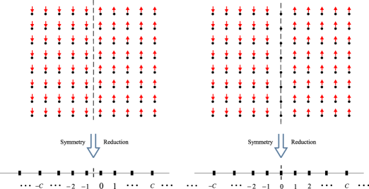
Figure 1: Reference configurations for the $180^{\circ}$ domain walls in the 2-D lattice of dipoles, their symmetry reduction and their reduced lattices. Left Panel: Type I, Right Panel: Type II.

For minimizing the free energy, first one should calculate the effective dynamical matrix according to Eq. (177). The calculations of this matrix for the two configurations are similar. For example, in configuration I due to symmetry we have $\mathbf{U}_{-1}=-\mathbf{U}_{0}$. Also we consider the temperature-dependent bulk configuration as the far-field condition, i.e., we assume $\mathbf{U}_{\alpha}=\mathbf{U}_{C}$ for $\alpha\geq C+1$. Our numerical experiments show that choosing $C=35$ would be enough to capture the structure of the atomic displacements near the defect, so we use $C=35$ in what follows. For the right half of the defective lattice we have

$$\mathbf{D}_{\ast\star}=\left(\begin{array}[]{ccccccc}\mathbf{E}^{\ast\star}_{0}&\mathbf{D}^{\ast\star}_{01}&\mathbf{0}_{2\times 2}&\ldots&\mathbf{0}_{2\times 2}&\mathbf{0}_{2\times 2}&\mathbf{0}_{2\times 2}\\ \mathbf{D}^{\ast\star}_{10}&\mathbf{D}^{\ast\star}_{11}&\mathbf{D}^{\ast\star}_{12}&\ldots&\mathbf{0}_{2\times 2}&\mathbf{0}_{2\times 2}&\mathbf{0}_{2\times 2}\\ \mathbf{0}_{2\times 2}&\mathbf{D}^{\ast\star}_{21}&\mathbf{D}^{\ast\star}_{22}&\ldots&\mathbf{0}_{2\times 2}&\mathbf{0}_{2\times 2}&\mathbf{0}_{2\times 2}\\ \vdots&\vdots&\vdots&\ddots&\vdots&\vdots&\vdots\\ \mathbf{0}_{2\times 2}&\mathbf{0}_{2\times 2}&\mathbf{0}_{2\times 2}&\ldots&\mathbf{D}^{\ast\star}_{\left(C-2\right)\left(C-2\right)}&\mathbf{D}^{\ast\star}_{\left(C-2\right)\left(C-1\right)}&\mathbf{0}_{2\times 2}\\ \mathbf{0}_{2\times 2}&\mathbf{0}_{2\times 2}&\mathbf{0}_{2\times 2}&\ldots&\mathbf{D}^{\ast\star}_{\left(C-1\right)\left(C-2\right)}&\mathbf{D}^{\ast\star}_{\left(C-1\right)\left(C-1\right)}&\mathbf{D}^{\ast\star}_{\left(C-1\right)C}\\ \mathbf{0}_{2\times 2}&\mathbf{0}_{2\times 2}&\mathbf{0}_{2\times 2}&\ldots&\mathbf{0}_{2\times 2}&\mathbf{D}^{\ast\star}_{C\left(C-1\right)}&\mathbf{F}^{\ast\star}_{C}\\ \end{array}\right)\in\mathbb{R}^{S\times S},$$ (189)

where $S=2\left(C+1\right)$,

$$\mathbf{E}^{\ast\star}_{0}=\mathbf{D}^{\ast\star}_{00}-\mathbf{D}^{\ast\star}_{0\left(-1\right)}~{}~{}~{}~{}~{}\text{and}~{}~{}~{}~{}~{}\mathbf{F}^{\ast\star}_{C}=\mathbf{D}^{\ast\star}_{CC}+\mathbf{D}^{\ast\star}_{C\left(C+1\right)}~{}~{}~{}~{}~{}~{}~{}\ast,\star=x,p.$$ (190)

Now one can use the above matrices to calculate the effective dynamical matrix. Note that as a consequence of considering interaction of order $m$, the dynamical matrix will be sparse, i.e., only a small number of elements are nonzero. As the dimension of the system increases, sparsity can be very helpful in the numerical computations [52].

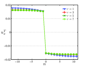
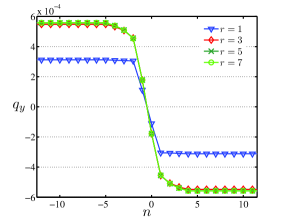
Figure 2: Position and polarization displacements for Type I domain wall ($\bar{T}=5$) obtained by choosing different number of $\mathbf{k}$-points ($r$) in the integration over the first Brillouin zone.

As was mentioned earlier, we will consider only the static part of the free energy to build the Hessian for the initial iteration and then update the Hessian using the BFGS algorithm in each step. To calculate the gradient of the free energy we need the third derivatives of the potential energy. These can be calculated using following relation

$$\frac{\partial\mathbf{D}}{\partial\boldsymbol{\Xi}}=\frac{\partial\mathbf{D}_{xx}}{\partial\boldsymbol{\Xi}}-\frac{\partial\mathbf{D}_{xp}}{\partial\boldsymbol{\Xi}}\mathbf{D}^{-1}_{pp}\mathbf{D}_{px}+\mathbf{D}_{xp}\mathbf{D}^{-1}_{pp}\frac{\partial\mathbf{D}_{pp}}{\partial\boldsymbol{\Xi}}\mathbf{D}^{-1}_{pp}\mathbf{D}_{px}-\mathbf{D}_{xp}\mathbf{D}^{-1}_{pp}\frac{\partial\mathbf{D}_{px}}{\partial\boldsymbol{\Xi}}~{}~{}~{}~{}~{}~{}~{}~{}~{}~{}\boldsymbol{\Xi}=\mathbf{X}^{i},\mathbf{\bar{P}}^{i}.$$ (191)

To obtain these third derivatives one can use the translation invariance relations (124) and (125) to simplify the calculations. For example, we can write

$$\frac{\partial^{3}\mathcal{E}}{\partial\mathbf{x}^{i}\partial\mathbf{x}^{i}\partial\mathbf{x}^{i}}\left(\mathcal{B}\right)=-\sideset{}{{}^{\prime}}{\sum}_{j\in\mathcal{L}_{i}}\frac{\partial^{3}\mathcal{E}}{\partial\mathbf{x}^{j}\partial\mathbf{x}^{i}\partial\mathbf{x}^{i}}\left(\mathcal{B}\right),$$ (192)

where a prime means that we exclude $j=i$ from the summation.

The dimensionalized temperature $\bar{T}$ and dimensionalized mass $\bar{m}$ correspond to the choice $\hbar=k_{B}=10^{-3}$. and work with normalized . To obtain the static equilibrium configuration and also in dynamic calculations we use $a=1.0$, $P_{0}=1.0$, $\epsilon=0.125$ , $K_{A}=2.0$ and $\bar{m}=10^{4}$. In what follows convergence tolerance for $\sqrt{\boldsymbol{\nabla}\mathcal{F}\cdot\boldsymbol{\nabla}\mathcal{F}^{\textsf{T}}}$ is $10^{-5}$. Using this value for convergence tolerance, solutions converge after ten to twenty iterations. In Fig. 2 we plot $u^{T}_{x}$ and $q_{y}$ for Type I domain wall and $\bar{T}=5$ for different number of $\mathbf{k}$-points ($r$) in the first Brillouin zone. Here $u^{T}_{x}$ is the diplacement of the lattice with respect to the nominal configuration at temperature $\bar{T}$. For numerical integrations over the first Brillouin zone we use the special points introduced in [46]. For the case $r=1$ we set $\mathbf{k}=0$, i.e., we assume that all of the atoms in a particular equivalence class vibrate with the same phase. As can be seen in these figures, displacements converge quickly by selecting $r=7$ $\mathbf{k}$-points in the first Brillouin zone, so in what follows we set $r=7$.

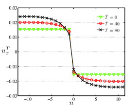
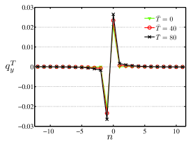
Figure 3: Position and polarization displacements of Type I domain wall with respect to the temperature-dependent nominal configurations.

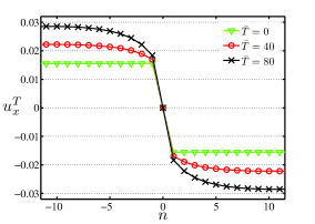
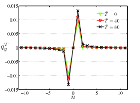
Figure 4: Position and polarization displacements of Type II domain wall with respect to the temperature-dependent nominal configurations.

Figs. 3 and 4 show the variations of displacements with temperature for the two domain walls. As temperature increases we cannot use the static equilibrium configuration as the reference configuration for calculating $\mathbf{H}_{0}$. Instead, we use the equilibrium configuration of a smaller temperature to obtain $\mathbf{H}_{0}$. Here, we use steps equal to $\Delta\bar{T}=5$. In other words, for calculating the structure of a domain wall at $\bar{T}=30$, for example, we use the structure at $\bar{T}=25$ as the initial configuration. We see that the lattice statics solution and the lattice configuration at $T=0$ obtained by the free energy minimization have a small difference. Such differences are due to the zero-point motions; the lattice statics method ignores the quantum effects. It is a well known fact that zero-point motions can have significant effects in some systems [31]. Note that polarization near the domain wall increases with temperature. Also as it is expected, the lattice expands by increasing the temperature.

Only a few layers around the domain wall are distorted; the rest of the lattice is displaced rigidly. As we see in Fig. 5, the domain wall thickness for both configurations increases as temperature increases. In this figure $\bar{w}_{T}=w_{T}/w_{0}$, where $w_{0}$ is the domain wall thickness at $\bar{T}=0$. Note also that in this temperature range $\bar{w}_{T}$ increases linearly with $\bar{T}$. This qualitatively agrees with experimental observations for PbTiO₃ in the low temperature regime [17]. Foeth, et al. [17] observed that domain wall thickness increases with temperature. What they measured was an average domain wall thickness. Note that domain wall thickness cannot be defined uniquely very much like boundary layer thickness in fluid mechanics. Here, domain wall thickness is by definition the region that is affected by the domain wall, i.e. those layers that are distorted. One can use definitions like the $99\%$-thickness in fluid mechanics and define the domain wall thickness as the length of the region that has $99\%$ of the far field rigid translation displacement. What is important is that no matter what definition is chosen, domain wall “thickness” increases by increasing temperature.

Our calculations show that by increasing the mass of the atoms both position and polarization displacements decrease. However, variations of displacements with respect to mass is very small. For example, by increasing mass from $\bar{m}=10^{4}$ to $\bar{m}=10^{6}$ at $\bar{T}=10$, displacements decrease by less than $0.1\%$.

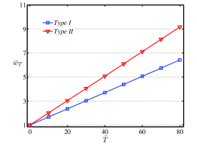
Figure 5: Variation of the $180^{\circ}$ domain wall thickness with temperature.

6 Concluding Remarks

In this paper we extended the classical method of lattice dynamics to defective crystals. The motivation for developing such a technique is to semi-analytically obtain the finite-temperature structure of defects in crystalline solids at low temperatures. Our technique exploits partial symmetries of defects. We worked out examples of defects in a 2-D lattice of interacting dipoles. We obtained the finite-temperature structure of two $180^{\circ}$ domain walls. We observed that using our simple model potential, increasing temperature domain walls thicken. This is in agreement with experimental results for ferroelectric domain walls in PbTiO₃. This technique can be used for many physically important material systems. Extending the present calculations for $180^{\circ}$ domain walls in PbTiO₃ will be the subject of a future work.

Appendix A The Ensemble Theories

There are different ensemble theories for calculating the thermodynamical properties of systems from the statistical mechanics point of view. In this appendix, we consider micro canonical and canonical ensemble theories and discuss the relation between them. In particular, we will see that the free energy minimization discussed in this paper is equivalent to finding the most probable energy at the given temperature. For more detailed discussions see [50].

A.1 Micro Canonical Ensemble Theory

From thermodynamical considerations, it is known that by specifying the limited number of properties of a system, one can determine all the other properties. In principle, any physical system, i.e., any macro system, consists of many smaller subsystems. Therefore, we can consider properties of each macro system as macrostates specified by the properties of these subsystems that are called microstates. Note that by a microstate we mean a set of values associated to each subsystem of a system. For example, consider an isolated system with energy $E$ and volume $V$ that consists of $N$ non-interacting particles with energies $\epsilon_{i}$, $i=1,2,\ldots,N$. Now each n-topple $(\epsilon_{1},\ldots,\epsilon_{i})$ satisfying

$$\sum_{i=1}^{N}\epsilon_{i}=E,$$ (193)

would represent a microstate of this system.

Obviously, there may exist several microstates that are associated to the same macrostate. Let $\Omega(E,N,V)$ denote the number of microstates associated with the given macrostate $(E,N,V)$. We assume that for an isolated system, (i) all microstate compatible with the given macrostates are equally probable, and (ii) equilibrium corresponds to the macrostate having the largest number of microstates. Let $S$ and $k_{B}$ denote the entropy of a system and Boltzmann constant, respectively. Then one can show that the above two assumptions and setting

$$S=k_{B}\ln(\Omega),$$ (194)

yields the equality of temperatures for systems that are in thermodynamical equilibrium. Note that (194) provides the fundamental relation between thermodynamics and statistical mechanics. Once $S$ is obtained, the derivation of other thermodynamical quantities would be a straight forward task.

A.2 Canonical Ensemble Theory

In practice, we never have an isolated system and even if we have such a system, it is hard to measure the total energy of the system. This means that it is more convenient to develop a statistical mechanics formalism that does not use $E$ as an independent variable. It is relatively easy to control the temperature of a system, i.e. we can always put the system in contact with a heat bath at temperature $T$. Thus, it is natural to choose $T$ instead of $E$.

Let a system be in equilibrium with a heat bath at temperature $T$ . In principle, the energy of the system at any instant of time can be equal to any energy level of the system. As a matter of fact, one can show that the probability of a system being in the energy level $P_{r}$ is equal to

$$P_{r}=\frac{g_{r}\exp(-E_{r}/k_{B}T)}{\sum_{i}g_{i}\exp(-E_{i}/k_{B}T)}=\frac{g_{r}\exp(-E_{r}/k_{B}T)}{Q(T,\Upsilon)},$$ (195)

where we define the partition function of the system as

$$Q(T,\Upsilon)=\sum_{i}g_{i}\exp(-E_{i}/k_{B}T),$$ (196)

and $\Upsilon$ denotes any other parameters that might govern the values of $E_{r}$. Note that the summation goes over all energy levels of the system and $g_{i}$ denotes the degeneracy of the state $E_{i}$, i.e. the number of different states associated with the energy level $E_{i}$. Thus, one may write $g_{i}=\Omega(E_{i})$, where $\Omega$ comes from the previous formulation. Assuming the total energy of the system to be an average energy of the different states, i.e.

$$E=\sum_{r}P_{r}E_{r},$$ (197)

one can show that the Helmholtz free energy $\mathcal{F}$ can be written as

$$\mathcal{F}=-k_{B}T\ln Q.$$ (198)

Equation (198) provides the basic relation in the canonical ensemble theory. Once $\mathcal{F}$ is known the other thermodynamic quantities can be easily obtained.

Note that we have chosen the average energy to be the energy of the system in this theory. One can show the total energy that we associate to the system on micro canonical ensemble theory corresponds to the most probable energy of the system, i.e. the energy level that maximizes $P_{r}$ at a given temperature $T$. In practice, i.e. in the thermodynamical limit $N\longrightarrow\infty$, it can be shown that these energies are equal and thus these two smilingly different approaches are the same.

Finally, note that

$$P_{r}=\frac{g_{r}\exp(-E_{r}/k_{B}T)}{Q(T,\Upsilon)}=\frac{\exp[-(E_{r}-k_{B}T\ln g_{r})/k_{B}T]}{Q(T,\Upsilon)}=\frac{\exp(-\mathcal{F}_{r}/k_{B}T)}{Q(T,\Upsilon)},$$ (199)

where we use $S=k_{B}\ln\Omega$, which is justified by the equivalence of the two ensemble theories. Equation (199) shows that to maximize $P_{r}$ at a fixed temperature, we need to minimize $\mathcal{F}_{r}$ over all admissible states $r$. To summarize, we have shown that minimizing the Helmholtz free energy at a temperature $T$ (and constant volume) is equivalent to finding the most probable energy level, which is the total energy of the system. Note that this minimization should be done over all variables that determine the free energy.

References

- [1] Allan, N. L. and Barrera, G. D. and Purton, J. A. and Sims, C. E. and Taylor, M. B. Ionic solids at elevated temperatures and/or high pressures: lattice dynamics, molecular dynamics, Monte Carlo and ab initio studies. Physical Chemistry Chemical Physics 2:1099-1111, 2000.
- Allan, et al. [1996] Allan, N. L. and Barron, T. H. K. and Bruno J. A. O. The zero static internal stress approximation in lattice dynamics, and the calculation of isotope effects on molar volumes. Journal of Chemical Physics 105:8300-8303, 1996.
- Born and Huang [1998] Born, M. and Huang, K. Dynamical Theory of Crystall Lattices. 1998.
- Boyer and Hardy [1971] Boyer, L. L., and J. R. Hardy. Lattice statics applied to screw dislocations in cubic metals. Philosophical Magazine, 24:647-671, 1971.
- Bullough and Tewary [1979] Bullough, R., and V. K. Tewary. Lattice theory of dislocations. In F. R. N. Nabarro, editor, Dislocations in Solids, North-Holland, 1970.
- Dick and Overhauser [1964] Dick, B. G. and A. W., Overhauser. Theory of the dielectric constants of alkali halide crystals. Physical Review, 112: 90-103, 1964.
- Diestler, et al. [2004] Diestler, D. J. and Wu, Z. B. and Zeng, X. C. An extension of the quasicontinuum treatment of multiscale solid systems to nonzero temperature. Journal of Chemical Physics 121:9279-9282, 2004.
- Dove [1993] Dove, M. T. Introduction to Lattice Dynamics. Cambridge University Press, 1993.
- Dupuy, et al. [2005] Dupuy, L., E. B. Tadmor, R. E. Miller, and R. Phillips. Finite temperature quasicontinuum: molecular dynamics without all the atoms. Physical Review Letters 95:060202, 2005.
- Esterling [1978a] Esterling, D. M. Equilibrium and Kinetic Aspects of Brittle-Fracture. International Journal of Fracture 14:417-427, 1978.
- Esterling [1978a] Esterling, D. M. Modified Lattice-Statics Approach to Dislocation Calculations .1. Formalism. Journal of Applied Physics 49:3954-3959, 1978.
- Esterling and Moriarty [1978] Esterling, D. M. and Moriarty, J. A. Modified Lattice-Statics Approach to Dislocation Calculations .2. Application. Journal of Applied Physics 49:3960-3966, 1978.
- Fernandez, et al. [2000] Fernandez, J. R. and Monti, A. M. and Pasianot, R. C. Vibrational entropy in static simulations of point defects. Physica Status Solidi B-Basic Research 219:245-251, 2000.
- Flocken and Hardy [1969] Flocken, J. W., and J. R. Hardy. Application of the method of lattice statics to vacancies in Na, K, Rb, and Cs. Physical Review 117:1054–1062, 1969.
- Flocken and Hardy [1970] Flocken, J. W., and J. R. Hardy. The Method of Lattice Statics. In H. Eyring and D. Henderson, editors, Fundamental Aspects of Dislocation Theory 1:219–245, 1970.
- Flocken [1972] Flocken, J. W. Modified lattice-statics approach to point defect calculations. Physical Review B, 6:1176–1181, 1972.
- Foeth, et al. [2007] Foeth, M., Stadelmann, P. and Robert, M. Temperature dependence of the structure and energy of domain walls in a first-order ferroelectric. Physica A 373:439-444, 2007.
- Foiles [1994] Foiles, S. M. Evaluation of harmonic methods for calculating the free-energy of defects in solids. Physical Review B 49:14930-14938, 1994.
- Forsblom, et al. [2004] Forsblom, M. and Sandberg, N. and Grimvall, G. Vibrational entropy of dislocations in Al. Philosophical Magazine 84:521-532, 2004.
- Gallego and Ortiz [1993] Gallego, R., and M. Ortiz. A harmonic/anharmonic energy partition method for lattice statics computations. Modelling and Simulation in Materials Sceince and Engineering 1:417–436, 1993.
- Guo, et al. [2005] Guo, W. L., Zhong, W. Y., Dai, Y. T. and Li, S. A. Coupled defect-size effects on interlayer friction in multiwalled carbon nanotubes. Physical Review B 72(7): 075409, 2005.
- Gutkin [2006] Gutkin, M. Y. Elastic behavior of defects in nanomaterials I. Models for infinite and semi-infinite media. Reviews on Advanced Materials Science 13:125-161, 2006.
- Hansen, et al. [1999] Hansen, U. and Vogl, P. and Fiorentini, V. Quasiharmonic versus exact surface free energies of Al: A systematic study employing a classical interatomic potential. Physical Review B, 60:5055-5064, 1999.
- Hsieh and Thomson [1973] Hsieh, C. and J. Thomson. Lattice theory of fracture and crack creep. Journal of Applied Physics 44:2051–2063, 1973.
- Jang and Farkas [2007] Jang, H. and Farkas, D. Interaction of lattice dislocations with a grain boundary during nanoindentation simulation. Material Letters 61(3):868-871, 2007.
- Kanazaki [1957] Kanazaki, H.. Point defects in face-centered cubic lattice-I Distortion around defects. Journal of Physics and Chemistry of Solids 2:24–36, 1957.
- Kantorovich [1995] Kantorovich, L. N. Thermoelastic properties of perfect crystals with nonprimitive lattices. I. General theory. Physical Review B 51(6):3520-3534, 1995.
- Kavianpour and Yavari [2009] Kavianpour, S. and Yavari A., Anharmonic analysis of defective crystals with many-body interactions using symmetry reduction. Computational Materials Science 44:1296-1306, 2009.
- Kesavasamy and Krishnamurthy [1978] Kesavasamy, K. and Krishnamurthy, N. Lattice-vibrations in a linear triatomic chain. American Journal of Physics 46:815-819, 1978.
- Kesavasamy and Krishnamurthy [1979] Kesavasamy, K. and Krishnamurthy, N. Vibrations of a one-dimensional defect lattice. American Journal of Physics 47:968-973, 1979.
- [31] Kohanoff, J. and Andreoni, W. and Parrinello, M. Zero-point-motion effects on the structure of C60. Physical Review B 46:4371-4373, 1992.
- Kittel [1987] Kittel, C. Quantum Theory of Solids. John Wiley & Sons, 1987.
- Kittel and Kroemer [1987] Kittel, C. and Kroemer, H. Thermal Physics. W.H. Freeman Company, 1980.
- Kiwi and Rossler [1972] Kiwi, M. and Rossler, J. Linear chain with free end boundary conditions. American Journal of Physics 40(1):143–151, 1972.
- Kossevich [1999] Kossevich, A. M. The Crystal Lattice. Wiley-VCH, 1999, Berlin.
- Kulkarni, et al. [2008] Kulkarni, Y., Knap, J. and Ortiz, M. A variational approach to coarse graining of equilibrium and non-equilibrium atomistic description at finite temperature. Journal of the Mechanics and Physics of Solids 56(4):1417-1449, 2008.
- Lacks andRutledge [1994] Lacks, D. J. and Rutledge, G. C. Implications of the volume dependent convergence of anharmonic free energy methods. Journal of Chemical Physics 101(11):9961-9965, 1994.
- Lesar, et al. [1989] Lesar, R. and Najafabadi, R. and Srolovitz, D. J. Finite-temperature defect properties from free-energy minimization. Physical Review Letters 63:624-627, 1989.
- de Lima, et al. [2008] de Lima, A. L. and Rosas, A. and Pedrosa, I. A. On the quantum motion of a generalized time-dependent forced harmonic oscillator. Annals of Physics 323(9):2253-2264, 2008.
- Maradudin [1958] Maradudin, A. A.. Screw dislocations and discrete elastic theory. Journal of the Physics and Chemistry of Solids 9:1–20, 1958.
- Matsubara [1952] Matsubara, T. J. Theory of diffuse scattering of X-rays by local lattice distortions. Journal of Physical Society of Japan 7:270-274, 1952.
- Meyer [1981] Meyer, H. D. On the forced harmonic oscillator with time-dependent frequency. Chemical Physics 61(3):365-383, 1981.
- Meyer and Vanderbilt [2001] Meyer, B. and Vanderbilt, D. Ab initio study of BaTiO3 and PbTiO3 surfaces in external electric fields. Physical Review B 63(20):205426, 2001.
- Maradudin, et al. [1971] Maradudin, A. A., E. W. Montroll, and G. H. Weiss. Theory of Lattice Dynamics in The Harmonic Approximation. Academic Press, 1971.
- Mok, et al. [2007] Mok, K. R. C., Colombeau, B., Benistant, F., et al. Predictive simulation of advanced Nano-CMOS devices based on kMC process simulation IEEE Transactions on Electron Devices 54(9):2155-2163, 2007.
- Monkhorst and Pack [1976] Monkhorst, H. J. and Pack, J. D. Special points for Brillouin-zone integrations. Physical Review B 13:5188-5192, 1976.
- [47] Nogami, Y. Test of the adiabatic approximation in quantum mechanics: Forced harmonic oscillator. American Journal of Physics 59(1):64–68, 1991.
- Ogata, et al. [2009] Ogata, S., Umeno, Y. and Kohyama, M. First-principles approaches to intrinsic strength and deformation of materials: perfect crystals, nano-structures, surfaces and interfaces. Modelling and Simulation in Materials Science and Engineering 17(1):013001, 2009.
- Ortiz and Phillips [1999] Ortiz, M. and R. Phillips. Nanomechanics of defects in solids. Advances in Applied Mechanics 59(1):1217–1233, 1999.
- Pathria [1996] Pathria, R. K. Statistical Mechanics. Elsevier, Oxford, 1996.
- Peierls [1955] Peierls, R. E. Quantum Theory of Solids. Oxford, 1955.
- Press, et al. [1989] Press, W. H., S. A. Teukolsky, W. T. Vetterling and B. P. Flannery. Numerical recipes: the art of scientific computing. Cambridge University Press, 1989.
- Rickman and LeSar [2002] Rickman, J. M. and LeSar, R. Free-energy calculations in materials research. Annual Review of Materials Research 32:195-217, 2002.
- Sanati and Esetreicher [2003] Sanati, M. and Esetreicher, S. K. Defects in silicon: the role of vibrational entropy. Solid State Communications 128:181-185, 2003.
- [55] Shenoy, V. B., M. Ortiz, and R. Phillips. The atomistic structure and energy of nascent dislocation loops. Modelling and Simulation in Materials Sceince and Engineering 7(4):603–619, 1999.
- Shukla and Cowley [1971] Shukla R. C., and Cowley, E. R. Helmholtz free energy of an anharmonic crystal to . Physical Review B 3:4055,1971.
- Tadmor, et al. [1996] Tadmor, E. B., M. Ortiz, and R. Phillips. Quasicontinuum analysis of defects in solids. Philosophical Magazine A 73(6):1529–1563, 1996.
- Tang, et al. [2006] Tang, Z. and Zhao, H. and Li, G. and Aluru, N. R. Finite-temperature quasicontinuum method for multiscale analysis of silicon nanostructures. Physical Review B 74:064110, 2006.
- Taylor, et al. [1999a] Taylor, M. B. and Allan, N. L. and Bruno, J. A. O. and Barrera, G. D. Quasiharmonic free energy and derivatives for three-body interactions. Physical Review B 59:353-363, 1999.
- Taylor, et al. [1997] Taylor, M. B. and Barrera, G. D. and Allan, N. L. and Barron, T. H. K. Free-energy derivatives and structure optimization within quasiharmonic lattice dynamics. Physical Review B 56:14380-14390, 1997.
- Taylor, et al. [1997] Taylor, M. B. and Barrera, G. D. and Allan, N. L. and Barron, T. H. K. and Mackrodt W. C. Free energy of formation of defects in polar solids. Faraday Discussion 106:377-387, 1997.
- Taylor, et al. [1999b] Taylor, M. B. and Sims, C. E. and Barrera, G. D. and Allan, N. L. and Mackrodt, W. C. Quasiharmonic free energy and derivatives for slabs: Oxide surfaces at elevated temperatures. Physical Review B 59:6742-6751, 1999.
- Tewary [2000] Tewary, V. K. Lattice-statics model for edge dislocation in crystals. Philosophical Magazine A 80:1445-1452, 2000.
- Tewary [1973] Tewary, V. K. Green-function method for lattice statics. Advances in Physics 22:757–810, 1973.
- Wallace [1965] Wallace, D. C. Lattice Dynamics and Elasticity of Stressed Crystals. 1965.
- Weiner [2002] Weiner, J. H. Statistical Mechanics of Elasticity. Dover, 2002.
- Westhaus [1981] Westhaus, P. A. Normal modes of a two-dimensional lattice of interacting dipoles. Journal of Biological Physics 9:169-190, 1981.
- Yavari, et al. [2005a] Yavari, A., M. Ortiz, and K. Bhattacharya. A theory of anharmonic lattice statics for analysis of defective crystals. Journal of Elasticity 86: 41-83, 2007.
- Yavari, et al. [2005b] Yavari, A., M. Ortiz, and K. Bhattacharya. Anharmonic lattice statics analysis of and ferroelectric domain walls in PbTiO3. Philosophical Magazine 87(26): 3997-4026, 2007.
- Zetterstrom, et al. [2005] Zetterstrom, P., Urbonaite, S, Lindberg, F, et al. Reverse Monte Carlo studies of nanoporous carbon from TiC. Journal OF Physics - Condensed Matter 17(23):3509-3524, 2005.
- Zhao, et al. [2006] Zhao, H. and Tang, Z. and Li, G. and Aluru, N. R. Quasiharmonic models for the calculation of thermodynamic properties of crystalline silicon under strain. Journal of Applied Physics 99, 2006.