Nonlinear and chaotic resonances in solar activity

Abstract

It is shown that, the wavelet regression detrended fluctuations of the monthly sunspot number for 1749-2009 years exhibit strong periodicity with a period approximately equal to 3.7 years. The wavelet regression method detrends the data from the approximately 11-years period. Therefore, it is suggested that the one-third subharmonic resonance can be considered as a background for the 11-years solar cycle. It is also shown that the broad-band part of the wavelet regression detrended fluctuations spectrum exhibits an exponential decay that, together with the positive largest Lyapunov exponent, are the hallmarks of chaos. Using a complex-time analytic approach the rate of the exponential decay of the broad-band part of the spectrum has been theoretically related to the Carrington solar rotation period. Relation of the driving period of the subharmonic resonance (3.7-years) to the active longitude flip-flop phenomenon, in which the dominant part of the sunspot activity changes the longitude every 3.7 years on average, has been briefly discussed.

Figure 1: The monthly sunspot number (dashed line) for the period 1749-2009 years. The data were taken from Ref. belg . The solid curve (trend) corresponds to a wavelet (symmlet) regression of the data.

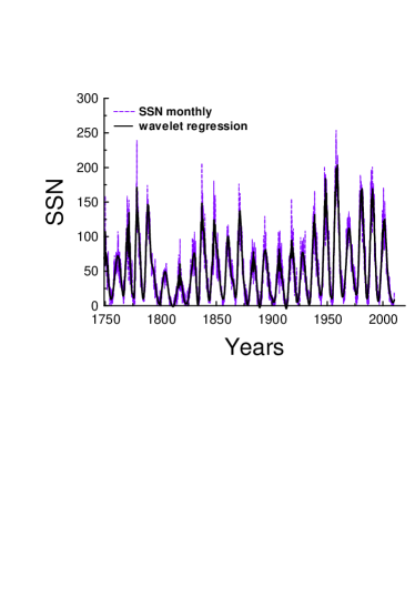
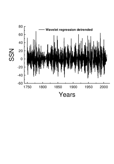
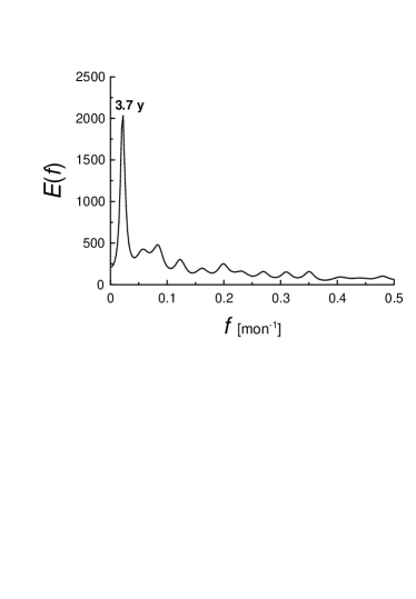
The solar activity is chaotic but has a well-defined mean period of about 11 years. The 11-year cycle is well known for more than a century and a half. Despite this, nature of the 11-year cycle is still unknown. Most of the regression methods are linear in responses and statistical analyses of the experimental sunspot data was dominated by linear stochastic methods, while it was recently rigorously shown in Ref. pn that a nonlinear dynamical mechanism (presumably a driven nonlinear oscillator) determines the sunspot cycle. Figure 1 shows the monthly sunspot number (dashed line) for the period 1749-2009 years (the data were taken from Ref. belg ). The solid curve (trend) corresponds to a wavelet (symmlet) regression of the data (cf. Ref. o ). Figure 2 shows corresponding detrended fluctuations, which produce a statistically stationary set of data. At the nonlinear nonparametric wavelet regression one chooses a relatively small number of wavelet coefficients to represent the underlying regression function. A threshold method is used to keep or kill the wavelet coefficients. In this case, in particular, the Universal (VisuShrink) thresholding rule with a soft thresholding function was used. At the wavelet regression the demands to smoothness of the function being estimated are relaxed considerably in comparison to the traditional methods. Figure 3 shows a spectrum of the wavelet regression detrended data calculated using the maximum entropy method (because it provides an optimal spectral resolution even for small data sets). In Fig. 3 one can see a well defined peak corresponding to period $\sim$ 3.7 years. The wavelet regression method detrends the data from the approximately 11-years period (cf. Fig. 1). Therefore, it is plausible that the one-third subharmonic resonance nm can be considered as a background for the 11-years solar cycle: $11/3.7\simeq 3$. Indeed, it is known nocera that interaction of the Alfven waves (generated in a highly magnetized plasma by a cavity’s moving boundaries) with slow magnetosonic waves can be described using Duffing oscillators (see also Refs. pn ,pl ). Let us imagine a forced excitable system with a large amount of loosely coupled degrees of freedom schematically represented by Duffing oscillators (which has become a classic model for analysis of nonlinear phenomena and can exhibit both deterministic and chaotic behavior nm ,ph depending on the parameters range) with a wide range of the natural frequencies $\omega_{0}$ :

$$\ddot{x}+\omega_{0}^{2}x+\gamma\dot{x}+\beta x^{3}=F\sin\omega t$$

where $\dot{x}$ denotes the temporal derivative of $x$, $\beta$ is the strength of nonlinearity, and $F$ and $\omega$ are characteristic of a driving force. It is known (see for instance Ref. nm ) that when $\omega\approx 3\omega_{0}$ and $\beta\ll 1$ the equation (1) has a resonant solution

$$x(t)\approx a\cos\left(\frac{\omega}{3}t+\varphi\right)+\frac{F}{(\omega^{2}-\omega_{0}^{2})}\cos\omega t$$

where the amplitude $a$ and the phase $\varphi$ are certain constants. This is so-called one-third subharmonic resonance with the driving frequency $\omega$ corresponding approximately to 3.7 years period (the peak in Fig. 3 corresponds to the second term in the right-hand side of the Eq. (2) while the first term has been detrended). For the considered system of the oscillators an effect of synchronization can take place and, as a consequence of this synchronization, the characteristic peaks in the spectra of partial oscillations coincide nl . It can be useful to note, for the solar activity modeling, that the odd-term subharmonic resonance is a consequence of the reflection symmetry of the natural nonlinear oscillators (invariance to the transformation $x\rightarrow-x$).

Figure 2: The wavelet regression detrended fluctuations from the data shown in Fig. 1.

Figure 3: Spectrum of the wavelet regression detrended fluctuations shown in Fig. 2.

Figure 4: The same as in Fig. 3 but in semi-logarithmical scales. The dashed straight line indicates an exponential decay.

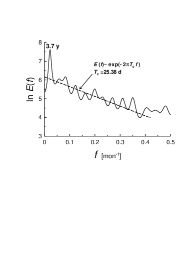
In order to understand appearance of the $3.7$-years period let us represent the spectrum shown in Fig. 3 in semi-logarithmical scales: figure 4. In these scales an exponential behavior corresponds to a straight line. It is known, that both stochastic and deterministic processes can result in the broad-band part of the spectrum, but the decay in the spectral power is different for the two cases. The exponential decay indicates that the broad-band spectrum for these data arises from a deterministic rather than a stochastic process. For a wide class of deterministic systems a broad-band spectrum with exponential decay is a generic feature of their chaotic solutions Refs. oht -fm . A wavy exponential decay (see Fig. 4) is a characteristic of a chaotic behavior generated by time-delay differential equations fa . A classic example of time-delay differential equation with chaotic solutions is the Mackey-Glass equation:

$$\frac{du(t)}{dt}=\frac{0.2\cdot u(t-\tau)}{(1+u(t-\tau)^{10})}-0.1\cdot u(t)$$

Figure 5 shows spectrum of a solution of this equation for the time-delay $\tau=30$. The dashed straight line indicates an exponential decay (cf. Fig. 4).

In the dynamo models that have physically distinct source layers the finite time is required in order to transport magnetic flux from one layer to another ws , it is especially significant for those dynamo models that have spatially segregated source regions for the poloidal and toroidal magnetic field components (such as, for instance, the Babcock- Leighton dynamo mechanism chau ). In the global dynamo models that include meridional circulation the time delay related to the circulation should be comparable to global rotation period (see below).

Nature of the exponential decay of the power spectra of the chaotic systems is still an unsolved mathematical problem. A progress in solution of this problem has been achieved by the use of the analytical continuation of the equations in the complex domain (see, for instance, fm ). In this approach the exponential decay of chaotic spectrum is related to a singularity in the plane of complex time, which lies nearest to the real axis (see the insert in Fig. 5). Distance between this singularity and the real axis determines the rate of the exponential decay. For many interesting cases chaotic solutions are analytic in a finite strip around the real time axis. This takes place, for instance for attractors bounded in the real domain (the Lorentz attractor, for instance). In this case the radius of convergence of the Taylor series is also bounded (uniformly) at any real time.

Let us consider, for simplicity, solution $u(t)$ with simple poles only, and to define the Fourier transform as follows

$$\tilde{u}(f)=(2\pi)^{-1/2}\int_{-T_{e}/2}^{T_{e}/2}dt~{}e^{-i2\pi ft}u(t)$$

Then using the theorem of residues

$$\tilde{u}(f)=i(2\pi)^{1/2}\sum_{j}R_{j}\exp(i2\pi fx_{j}-|2\pi fy_{j}|)$$

where $R_{j}$ are the poles residue and $x_{j}+iy_{j}$ are their location in the relevant half plane, one obtains asymptotic behavior of the spectrum $E(f)=|\tilde{u}(f)|^{2}$ at large $f$

$$E(f)\sim\exp(-4\pi|y_{min}|~{}f)$$

where $y_{min}$ is the imaginary part of the location of the pole which lies nearest to the real axis. In the case of symmetric analytic strip with a width $\Delta=2|y_{min}|$:

$$E(f)\sim\exp(-2\pi\Delta~{}f)$$

(cf. the insert in Fig. 5).

Figure 5: Spectrum of the Mackey-Glass chaotic time-series. The dashed straight line indicates an exponential decay. The insert shows a sketch of corresponding complex-time plane.

Figure 6: The pertaining average maximal Lyapunov exponent at the pertaining time, calculated for the same data as those used for calculation of the spectrum (Figs. 3 and 4). The dashed straight line indicates convergence to a positive value.

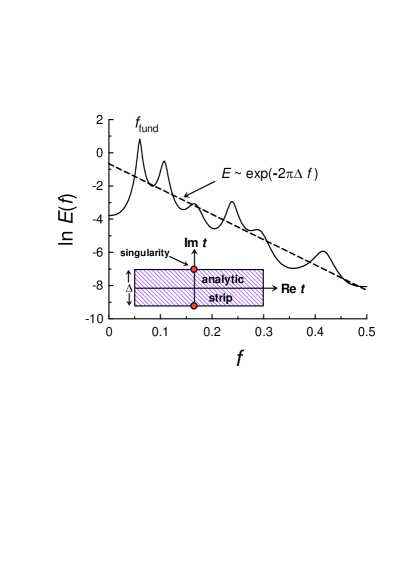
The chaotic spectrum provides two different characteristic time-scales for the chaotic system: a period corresponding to fundamental frequency of the system, $f_{fund}$, and a period corresponding to the exponential decay rate, $2\pi\Delta$ (cf. Eq. (5)). The fundamental period can be estimated using position of the low-frequency peak (cf. Figs. 4 and 5), while the exponential decay rate period $2\pi\Delta$ can be estimated using the slope of the straight line of the broad-band part of the spectrum in the semi-logarithmic representation. In the case of the global solar dynamo the width of the analytic strip $\Delta$ can be theoretically estimated using the Carrington solar rotation period: $\Delta\simeq T_{c}\simeq 25.38$ days. This period roughly corresponds to the solar rotation at a latitude of 26 deg, which is consistent with the typical latitude of sunspots (cf. Fig. 4).

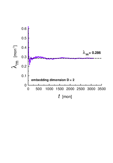
Additionally to the exponential spectrum (Fig. 4), let us check the chaotic character of the wavelet regression detrended fluctuations calculating the largest Lyapunov exponent: $\lambda_{max}$. A strong indicator for the presence of chaos in the examined time series is condition $\lambda_{max}>0$. If this is the case, then we have so-called exponential instability. Namely, two arbitrary close trajectories of the system will diverge apart exponentially, that is the hallmark of chaos. To calculate $\lambda_{max}$ we used a direct algorithm developed by Wolf et al. w . Figure 6 shows the pertaining average maximal Lyapunov exponent at the pertaining time, calculated for the data set shown in Fig. 2. The largest Lyapunov exponent converges very well to a positive value $\lambda_{max}\simeq 0.286~{}mon^{-1}>0$.

It should be noted that the same period $\sim 3.7$ years was recently found for the so-called flip-flop phenomenon of the active longitudes in solar activity bu ,bu2 . Sunspots are tend to pop up preferably in certain latitudinal domains and move toward the equator due to the 11-year cycle. Recently, strong indications of non-uniform longitudinal distribution of sunspots (active longitudes) was reported and analyzed in a dynamic frame related to the mean latitude of sunspot formation, in which the active longitudes persist for the last eleven solar 11-years cycles (see Refs. bu ,bu2 and references therein). At any given time, one of the two active longitudes (approximately $180^{0}$ apart) exhibits a stronger activity - dominance. Observed alternation of the active longitudes dominance in 3.7 years on average was called as flip-flop phenomenon bu . It seems rather plausible that the observed flip-flop period and the period of the wavelet regression detrended fluctuations of solar activity (Fig. 4) have the same origin. In this vein, the observation bu ,mh that the period of the flip-flop phenomenon follows to variations of the real length of the sunspot cycle (which has the 11-years period on average only) supports the idea of the one-third subharmonic resonance as a background of the 11-years cycle of solar activity.

The author is grateful to SIDC-team, World Data Center for the Sunspot Index, Royal Observatory of Belgium for sharing their data. A software provided by K. Yoshioka was used at the computations.

References

- (1) M. Palus, and D. Novotna, Sunspot Cycle: A Driven Nonlinear Oscillator?, Phys. Rev. Lett., 83, 3406-3409 (1999).
- (2) The data are available at http://sidc.oma.be/sunspot-data/
- (3) T. Ogden, Essential Wavelets for Statistical Applications and Data Analysis (Birkhauser, Basel, 1997).
- (4) A.H. Nayfeh and D.T. Mook, ”Nonlinear Oscillations” (John Wiley & Sons, a Wiley-Interscience Publication, 1979).
- (5) L. Nocera, Subharmonic oscillations of a forced hydromagnetic cavity, Geoph. & Astroph. Fluid Dynamics, 76, 239-252 (1994).
- (6) D. Passos and I. Lopes, A Low-Order Solar Dynamo Model: Inferred Meridional Circulation Variations Since 1750, ApJ 686 142
- (7) D. Permann and I. Hamilton, Wavelet analysis of time series for the Duffing oscillator: The detection of order within chaos, Phys. Rev. Lett., 69, 2607 (1992).
- (8) Yu.I. Neimark and P.S. Landa, Stochastic and Chaotic Oscillations, (Dordrecht, Kluwer, 1992).
- (9) N. Ohtomo, et. al., Exponential Characteristics of Power Spectral Densities Caused by Chaotic Phenomena, J. Phys. Soc. Jpn., 64, 1104-1113 (1995).
- (10) J. D. Farmer, Chaotic attractors of an infinite dimensional dynamic system, Physica D, 4, 366-393 (1982).
- (11) D.E. Sigeti, Survival of deterministic dynamics in the presence of noise and the exponential decay of power spectrum at high frequencies. Phys. Rev. E, 52, 2443-2457 (1995).
- (12) U. Frisch and R. Morf, Intermittency in non-linear dynamics and singularities at complex times, Phys. Rev. 23, 2673 (1981).
- (13) A.L. Wilmot-Smith et al., A time delay model for solar and stellar dynamos, ApJ, 652 696-708 (2006).
- (14) P. Charbonneau, C. St-Jean, and P. Zacharias, Fluctuations in Babcock-Leighton dynamos, I. Period doubling and transition to chaos, ApJ, 619 613-622 (2005).
- (15) A. Wolf et al., Determining Lyapunov exponents from a time series, Physica D, 16, 285-317 (1985).
- (16) S.V. Berdyugina and I.G. Usoskin, Active longitudes in sunspot activity: Century scale persistence, A&A 405, 1121-1128 (2003).
- (17) I.G. Usoskin, S.V. Berdyugina, D. Moss, and D.D. Sokoloff, Long-term persistence of solar active longitudes and its implications for the solar dynamo theory, Advances in Space Research, 40, 951-958 (2007).
- (18) K. Mursula, and T. Hiltula, Systematically asymmetric heliospheric magnetic field: evidence for a quadrupole mode and non-axisymmetry with polarity flip flops, Solar Phys. 224, 133 (2004).