Renormalization group running of neutrino parameters
in the inverse seesaw model

Abstract

We perform a detailed study of the renormalization group equations in the inverse seesaw model. Especially, we derive compact analytical formulas for the running of the neutrino parameters in the standard model and the minimal supersymmetric standard model, and illustrate that, due to large Yukawa coupling corrections, significant running effects on the leptonic mixing angles can be naturally obtained in the proximity of the electroweak scale, perhaps even within the reach of the LHC. In general, if the mass spectrum of the light neutrinos is nearly degenerate, the running effects are enhanced to experimentally accessible levels, well suitable for the investigation of the underlying dynamics behind the neutrino mass generation and the lepton flavor structure. In addition, the effects of the seesaw thresholds are discussed, and a brief comparison to other seesaw models is carried out.

I Introduction

Experimental progress on neutrino masses and leptonic mixing has opened up a new window in searching for new physics beyond the standard model (SM) of particle physics during the past decade. Since neutrinos are massless particles in the SM, one usually extends the SM particle content in order to accommodate massive neutrinos. Among various theories of this kind, the seesaw mechanism Minkowski (1977); *Yanagida:1979as; *GellMann:1980vs; *Mohapatra:1979ia; *Magg:1980ut; *Schechter:1980gr; *Wetterich:1981bx; *Lazarides:1980nt; *Mohapatra:1980yp; *Cheng:1980qt; *Foot:1988aq attracts a lot of attention in virtue of its naturalness and simplicity. For instance, in the conventional type-I seesaw model, three right-handed neutrinos with a Majorana mass term far above the electroweak scale are introduced. The masses of the light neutrinos are then strongly suppressed with respect to the masses of the charged leptons by the ratio between the electroweak scale and the mass scale of the heavy right-handed neutrinos. Usually, the neutrino parameters are measured in low-energy scale experiments, while on the other hand, the seesaw-induced neutrino mass operator often emerges at some very high-energy scale. Therefore, neutrino masses and leptonic mixing parameters are subject to radiative corrections, i.e., they are modified by the renormalization group (RG) running. In principle, the RG running effects can even be physically relevant, especially if the seesaw scale turns out to be not extremely high.

The generic features of the RG running of neutrino parameters have been investigated intensively in the literature. Typically, at energy scales lower than the seesaw threshold, i.e., the mass scale of the heavy seesaw particles, the RG running behavior of neutrino masses and leptonic mixing can be described within an effective theory, which is essentially the same for various seesaw models, reflecting the uniqueness of the dimension-five Majorana mass operator in the SM. However, at energy scales higher than the seesaw threshold, a full theory has to be considered, and the interplay between the light and heavy sectors could make the RG running effects particularly different compared to those in the effective theory. The RG running effects above the seesaw scale are especially relevant in the wide class of popular theories based on the idea of grand unification, i.e. grand unification theory (GUT), where the specific flavor structure stipulated at the GUT scale, typically of the order of $10^{16}$ GeV, often experiences a long range running over many intermediate energy-scale thresholds.

Concerning any specific seesaw model, a generic analysis of the RG running of neutrino parameters is clearly inconceivable because of an infinite number of possible underlying models, in particular, above the relevant seesaw threshold. Nevertheless, the universal features, like the presence of extra degrees of freedom underpinning the seesaw, i.e., the heavy fermions in the type-I and -III models or the scalar triplets in the type-II seesaw model, and the nature of their interactions with the SM sector, still admit for a high degree of theoretical scrutiny, providing a basis for any further work within a specific class of unified models.

The full set of renormalization group equations (RGEs) in the type-I, -II, and -III seesaw models have been derived, both in the SM and in the minimal supersymmetric standard model (MSSM) Chankowski and Pluciennik (1993); *Babu:1993qv; *Antusch:2001ck; *Antusch:2001vn; Rossi (2002); *Joaquim:2009vp; Chao and Zhang (2007); *Schmidt:2007nq; Chakrabortty et al. (2009). However, in these models, the seesaw scale is often taken not too far below the GUT scale, which hinders the direct experimental testability of the origin of neutrino masses. Although, in the type-I seesaw model, one can bring down the mass scale of the right-handed neutrinos by means of a severe fine-tuning among the model parameters Pilaftsis (1992); *Kersten:2007vk; *Antusch:2009gn; *Zhang:2009ac, radiative corrections induced by right-handed neutrinos tend to spoil the stability of such settings beyond the tree-level approximation.

Recently, a lot of attention has been focused on low-scale seesaw models, and especially, the possibility of searching for seesaw particles at the Large Hadron Collider (LHC), see, e.g., Ref. Nath et al. (2009) and references therein. In these models, the smallness of the neutrino masses is protected by other means than the GUT-scale suppression, such as a small amount of lepton number breaking. A very attractive example along this direction is the inverse seesaw model Mohapatra and Valle (1986), in which the light neutrino masses are driven by a tiny Majorana mass insertion in the heavy Dirac neutrino mass matrix instead of the mass scale of the heavy neutrinos. Furthermore, due to the pseudo-Dirac feature of the heavy singlets, the model does not suffer from either large radiative corrections or unnatural fine-tuning problems. This admits for bringing the heavy neutrinos down to the LHC energy range while retaining potentially large Yukawa couplings. Subsequently, this makes the model phenomenologically very attractive from the lepton flavor violation point of view Bernabeu et al. (1987) or for the potentially large nonunitarity effects in the leptonic mixing matrix Antusch et al. (2006). Since the RG running, and in particular, the threshold effects, in such a scenario can play an important role even at a relatively low energy scale, there is a need to look in detail at the running effects on neutrino parameters.

In this work, we will investigate in detail the RG evolution of neutrino masses and leptonic mixing parameters in the inverse seesaw model. In particular, in Sec. II, we first review briefly the inverse seesaw model. Next, in Sec. III, we present the full set of RGEs for the neutrino parameters. Then, in Sec. IV, we provide useful approximations of the RGEs found in Sec. III. Section V is devoted to detailed numerical illustrations and interpretation of the RG running behavior of the light neutrino mass and leptonic mixing parameters. In Sec. VI, a discussion and comparisons between RGEs in various seesaw models are performed. Finally, in Sec. VII, a summary is given and our conclusions are presented. In addition, in App. A, the complete one-loop RGEs for some of the neutrino parameters are listed.

II The inverse seesaw model

The inverse seesaw model is constructed by extending the SM particle content with three right-handed neutrinos $\nu_{\rm R}=(\nu_{\rm R1},\nu_{\rm R2},\nu_{\rm R3})$ and three SM gauge singlets $S=(S_{1},S_{2},S_{3})$. The Lagrangian of the lepton masses is then arranged so that it reads in flavor basis

$$-{\cal L}_{\nu}=\overline{\ell_{\rm L}}\phi Y_{e}e_{\rm R}+\overline{\ell_{\rm L}}\tilde{\phi}Y_{\nu}\nu_{\rm R}+\overline{S^{c}}M_{\rm R}\nu_{\rm R}+\frac{1}{2}\overline{S^{c}}M_{S}S+{\rm h.c.}\,,$$ (1)

where $\phi$ is the SM Higgs fields with $\tilde{\phi}={\rm i}\tau_{2}\phi^{*}$, $M_{\rm R}$ is an arbitrary $3\times 3$ matrix, and $M_{S}$ is a $3\times 3$ complex symmetric matrix. Here $Y_{e}$ and $Y_{\nu}$ are the corresponding Yukawa coupling matrices, and in general, they are arbitrary. Without loss of generality, due to the freedom in the right-handed fields, one can always perform basis transformations to keep both $M_{\rm R}$ and $Y_{e}$ diagonal, i.e., $M_{\rm R}={\rm diag}(M_{1},M_{2},M_{3})$ and $Y_{e}={\rm diag}(y_{e},y_{\mu},y_{\tau})$. Since the new extra fermions are SM gauge singlets, their masses are not protected by the Higgs mechanism, and could be related with some new physics beyond the SM. Thus, one expects the scale of heavy seesaw particles to be higher than the electroweak scale, i.e., $M_{\rm R}>{\cal O}(100)~{}{\rm GeV}$. At energy scales lower than $M_{\rm R}$, heavy degrees of freedom in the theory should be integrated out, which leaves a series of higher-dimensional nonrenormalizable operators in the effective theory. At dimension-five level, the only allowed operator is the so-called Weinberg operator, coupling two lepton doublets to the SM Higgs field, on the form

$${\cal L}^{d=5}_{\nu}=-\frac{1}{2}(\overline{\ell_{\rm L}}\phi)\cdot\kappa\cdot(\phi^{T}\ell^{c}_{\rm L})+{\rm h.c.}\,,$$ (2)

where $\kappa$ is the effective coupling matrix. In the inverse seesaw model and at tree-level, it is given by

$$\kappa\simeq Y_{\nu}M^{-1}_{\rm R}M_{S}(M^{T}_{\rm R})^{-1}Y^{T}_{\nu}\,.$$ (3)

After electroweak symmetry breaking, the dimension-five operator defined in Eq. (2) yields an effective Majorana mass term for the light neutrinos

$$m_{\nu}=\kappa v^{2}\,,$$ (4)

with $v\simeq 174~{}{\rm GeV}$ being the vacuum expectation value of the Higgs doublet.

Comparing Eq. (3) with the typical type-I seesaw model, in which the effective coupling matrix $\kappa$ is given by $\kappa\simeq Y_{\nu}M^{-1}_{\rm R}Y^{T}_{\nu}$, one can observe that, in the inverse seesaw, the masses of the light neutrinos are not only suppressed by $M_{\rm R}$, but also by the small Majorana insertion $M_{S}$. In the limit $M_{S}\to 0$, $\kappa=0$ indicates the restoration of lepton number conservation, which in turn ensures the naturalness of a tiny $M_{S}$.

Now, since the energy scale of $M_{\rm R}$ is not necessarily high, we may naturally ask if it is related to some new physics around the TeV scale and could be tested at the current hadron colliders (e.g., LHC). In fact, for the purpose of searching for heavy singlets at colliders, it is very important to have visible mixing effects between the light and heavy neutrinos. Furthermore, the admixture results in nonunitarity effects in neutrino flavor transitions, especially for some of the future long-baseline neutrino oscillation experiments Antusch et al. (2006); Antusch et al. (2009a); Malinský et al. (2009, 2009); Fernández-Martínez et al. (2007); *Abada:2007ux; *Xing:2007zj; *Goswami:2008mi; *Luo:2008vp; *Altarelli:2008yr; *Antusch:2009pm; *Rodejohann:2009cq.

In spite of the underlying physics responsible for large neutrino masses, the particle content of the inverse seesaw model is essentially the same as that of the type-I seesaw model, but with six right-handed neutrinos. In principle, one may treat the heavy singlets $S_{i}$ ($i=1,2,3$) as three extra right-handed neutrinos, possessing vanishing Yukawa couplings with the lepton doublets. In the limit $M_{S}\to 0$, lepton number conservation is restored, and the six heavy singlets can be combined together to form three four-component Dirac particles, while keeping the light neutrinos massless. Therefore, any phenomena in association with lepton number violation should be proportional to the Majorana mass insertion $M_{S}$.

III RGEs for the neutrino mass matrix

As discussed above, the analogy between the type-I seesaw model and the inverse seesaw model allows us to readily write down the RGEs for the Yukawa couplings and the neutrino mass matrix from the existing RGEs of the type-I seesaw model Chankowski and Pluciennik (1993); *Babu:1993qv; *Antusch:2001ck; *Antusch:2001vn. Especially, the relevant beta functions, obtained using the minimal subtraction renormalization scheme, are given by

$$16\pi^{2}\mu\frac{{\rm d}Y_{e}}{{\rm d}\mu} = \left(\alpha_{e}+C^{e}_{e}X_{e}+C^{\nu}_{e}X_{\nu}\right)Y_{e}\,,$$ (5)

$$16\pi^{2}\mu\frac{{\rm d}Y_{\nu}}{{\rm d}\mu} = \left(\alpha_{\nu}+C^{e}_{\nu}X_{e}+C^{\nu}_{\nu}X_{\nu}\right)Y_{\nu}\,,$$ (6)

$$16\pi^{2}\mu\frac{{\rm d}M_{\rm R}}{{\rm d}\mu} = C_{\rm R}M_{\rm R}Y^{\dagger}_{\nu}Y_{\nu}\,,$$ (7)

$$16\pi^{2}\mu\frac{{\rm d}M_{S}}{{\rm d}\mu} = 0\,,$$ (8)

where $\mu$ is the renormalization scale, $Y_{f}$ (for $f=u,d,e,\nu$) denote the Yukawa coupling matrices with $X_{f}=Y_{f}Y^{\dagger}_{f}$. The coefficients $(C^{e}_{e},C^{\nu}_{e},C^{e}_{\nu},C^{\nu}_{\nu},C_{\rm R})$ stand for $(3/2,-3/2,-3/2,3/2,1)$ in the SM and $(3,1,1,3,2)$ in the MSSM, respectively. The coefficient $\alpha_{\nu}$ is flavor blind and reads

$$\alpha_{\nu}={\rm tr}\left(3X_{u}+3X_{d}+X_{e}+X_{\nu}\right)-\frac{9}{20}g^{2}_{1}-\frac{9}{4}g^{2}_{2}$$ (9)

in the SM, and

$$\alpha_{\nu}={\rm tr}\left(3X_{u}+X_{\nu}\right)-\frac{3}{5}g^{2}_{1}-3g^{2}_{2}$$ (10)

in the MSSM with $g_{i}$ being the gauge couplings. Then, if we make use of $m_{\nu}$ at energy scales above the seesaw threshold, we can derive from Eqs. (3) and (5)-(8)

$$\frac{{\rm d}m_{\nu}}{{\rm d}t}\equiv\dot{m}_{\nu}=2\alpha_{\nu}m_{\nu}+\left(C^{e}_{\nu}X_{e}+C_{m}X_{\nu}\right)m_{\nu}$$ (11)

$$+m_{\nu}\left(C^{e}_{\nu}X_{e}+C_{m}X_{\nu}\right)^{T}\,,$$ (12)

with $C_{m}=1/2$ in the SM and $C_{m}=1$ in the MSSM. Here, for simplicity, we have defined $t=1/(16\pi^{2})\ln(\mu/M_{Z})$.

The beta functions in Eqs. (5)-(8) are obtained in the minimal subtraction renormalization scheme, and thus, we use an effective theory below the seesaw thresholds, in which the heavy fields are absent and their physical effects are covered by a series of higher-dimensional operators. To ensure that the full and the effective theories give identical predictions for physical quantities at low-energy scales, the parameters of the full and the effective theories have to be related to each other.

In the case of the neutrino mass matrix, this means relations between the effective coupling matrix $\kappa$ and the parameters $Y_{\nu}$, $M_{\rm R}$, and $M_{S}$ of the full theory. This is technically called matching between the full and the effective theories. In the effective theory, the Weinberg operator (2), responsible for the masses of the light neutrinos, does not depend on the specific seesaw realization and its evolution equation reads

$$\dot{\kappa}=\alpha_{\kappa}\kappa+\left(C^{e}_{\nu}X_{e}\right)\kappa+\kappa\left(C^{e}_{\nu}X_{e}\right)^{T}\,,$$ (13)

where

$$\alpha_{\kappa} = 2\>{\rm tr}\left(3X_{u}+3X_{d}+X_{e}\right)+\lambda-3g^{2}_{2}\,,\qquad\text{(in the SM)}$$ (14)

$$\alpha_{\kappa} = {\rm tr}\left(6X_{u}\right)-\frac{6}{5}g^{2}_{1}-6g^{2}_{2}\,,\qquad\text{(in the MSSM)}$$ (15)

with $\lambda$ denoting the SM Higgs self-coupling constant.

For the simplest case, if the mass spectrum of the heavy singlets is degenerate, namely $M_{1}=M_{2}=M_{3}=M_{0}$, one can simply make use of the tree-level matching condition

$$\kappa|_{\mu}=Y_{\nu}M^{-1}_{\rm R}M_{S}(M^{T}_{\rm R})^{-1}Y^{T}_{\nu}|_{\mu}\,$$ (16)

at the energy scale $\mu=M_{0}$. In the most general case with nondegenerate heavy singlets, i.e., $M_{1}<M_{2}<M_{3}$, the situation becomes more complicated and the heavy singlets have to be sequentially decoupled from the theory Antusch et al. (2002b). For instance, at energy scales between the $n$th and $(n-1)$th thresholds, the heavy singlets are partially integrated out, leaving only a $3\times(n-1)$ submatrix in $Y_{\nu}$, which is nonvanishing in the basis, where the heavy singlet mass matrix is diagonal. The decoupling of the $n$th heavy singlet leads to the appearance of an effective dimension-five operator similar to that in Eq. (2), and the effective neutrino mass matrix below $M_{n}$ is described by two parts

$$m^{(n)}_{\nu}=v^{2}\left[\kappa^{(n)}+Y_{\nu}^{(n)}\left(M_{\rm R}^{(n)}\right)^{-1}M_{S}^{(n)}\left(M_{\rm R}^{(n)T}\right)^{-1}Y_{\nu}^{(n)T}\right]\,,$$ (17)

where $(n)$ labels the quantities relevant for the effective theory between the $n$th and $(n-1)$th threshold. In the SM, the RGEs for the two terms above have different coefficients for the gauge coupling and Higgs self-coupling contributions, which can be traced back to the decoupling of the right-handed neutrinos from the theory. However, such a mismatch is absent in the MSSM due to the supersymmetric structure of the MSSM Higgs and gauge sectors. Therefore, this feature may result in significant RG running effects only in the SM, in particular, when the mass spectrum of the heavy neutrinos is quite hierarchical.

IV Analytical RGEs for neutrino parameters

In order to analytically investigate the RG evolution of leptonic mixing angles, CP-violating phases, and neutrino masses, one can translate the full RGEs for the neutrino mass matrix into a system of differential equations for these parameters. The corresponding formulas have been discussed below the seesaw scale Casas et al. (2000); *Chankowski:1999xc; *Antusch:2003kp, as well as above the seesaw thresholds in the type-I Antusch et al. (2005); *Mei:2005qp, -II Chao and Zhang (2007); *Schmidt:2007nq, and -III Chakrabortty et al. (2009) seesaw models.

In general, there are two different strategies for solving the resulting system. In the top-down approach, the initial condition is specified at a certain high-energy scale, often motivated by the flavor structure of a specific GUT-scale scenario. This is an advantage, since all the necessary ingredients are fixed at the high-energy scale and the running down to the electroweak scale is a mere tedium. On the other hand, only some regions in the parameter space of the full theory would presumably lead to good fits of the low-energy data, which, together with an ab initio model dependency, makes this method potentially quite inefficient.

In this study, we instead adopt the bottom-up approach, in which the initial condition for the observables of our interest is fixed at the low-energy scale, thus exploiting all the available experimental information from the beginning. It is also clear from the mere parameter counting that at the matching scale one can determine the underlying theory parameters only up to an equivalence class defined by the matching condition, and thus, the model-dependency problem is somewhat delayed. Nevertheless, in order to set off from the threshold, a representative should be chosen, which amounts to adding extra assumptions on the flavor structure of the underlying theory at the matching point. For a more detailed discussion on these issues, see e.g. Ref. Davidson and Ibarra (2001) and references therein.

In particular, one can make use of some of the qualitative features of the RGEs of the full theory. For instance, in the type-I seesaw model, the structure of Eqs. (5)-(8) and (11) justifies the typical diagonality assumption made on $Y_{\nu}$. Indeed, if both $Y_{e}$ and $Y_{\nu}$ are diagonal at a common energy scale, then they will retain the one-loop diagonality at any energy scale, since there is no nondiagonal element in the RGEs for $Y_{e}$ and $Y_{\nu}$. Thus, for the sake of simplicity, we assume $Y_{\nu}={\rm diag}(y_{\nu 1},y_{\nu 2},y_{\nu 3})$ in the basis in which $Y_{e}$ is also diagonal, which is reflected by the fact that from now on we work with just three combinations of the leptonic Yukawa couplings, namely

$$(y^{2}_{1},y^{2}_{2},y^{2}_{3})=C^{e}_{\nu}(y^{2}_{e},y^{2}_{\mu},y^{2}_{\tau})+C_{m}(y^{2}_{\nu 1},y^{2}_{\nu 2},y^{2}_{\nu 3}).$$ (18)

We will briefly comment on the general case with a nondiagonal Yukawa coupling matrix $Y_{\nu}$ later in Sec. V.4. The leptonic mixing matrix corresponds then to the unitary matrix $U$ diagonalizing $\kappa$ as

$$\kappa=U{\rm diag}(k_{1},k_{2},k_{3})U^{T}\,,$$ (19)

where $k_{i}$ ($i=1,2,3$) are the eigenvalues of $\kappa$. It is usually given using the standard parametrization

$$U = P_{\phi}\left(\begin{matrix}c_{12}c_{13}&s_{12}c_{13}&s_{13}e^{-{\rm i}\delta}\cr-s_{12}c_{23}-c_{12}s_{23}s_{13}e^{{\rm i}\delta}&c_{12}c_{23}-s_{12}s_{23}s_{13}e^{{\rm i}\delta}&s_{23}c_{13}\cr s_{12}s_{23}-c_{12}c_{23}s_{13}e^{{\rm i}\delta}&-c_{12}s_{23}-s_{12}c_{23}s_{13}e^{{\rm i}\delta}&c_{23}c_{13}\end{matrix}\right)\left(\begin{matrix}e^{{\rm i}\rho}&&\cr&e^{{\rm i}\sigma}&\cr&&1\end{matrix}\right)\ ,$$ (20)

with $c_{ij}\equiv\cos\theta_{ij}$ and $s_{ij}\equiv\sin\theta_{ij}$ ($ij=12$, $13$, $23$). Here $P_{\phi}={\rm diag}(e^{{\rm i}\phi_{1}},e^{{\rm i}\phi_{2}},e^{{\rm i}\phi_{3}})$ denotes three unphysical phases, which are required for the diagonalization of an arbitrary complex symmetric matrix.

For the RG running of leptonic mixing angles and CP-violating phases, in order to simplify the results, we define the quantities

$$\zeta_{ij}=\frac{m_{i}-m_{j}}{m_{i}+m_{j}}\,.$$ (21)

Inserting Eqs. (19) and (21) into Eq. (11) and using Eq. (18), we arrive after some tedious calculations at the RGEs for the leptonic mixing angles and the CP-violating phases in the current scheme. The explicit, but rather cumbersome results, are shown in App. A.

In the case that the mass spectrum of the light neutrinos is nearly degenerate, i.e., $m_{1}\simeq m_{2}\simeq m_{3}$, one can expect large enhancement factors $\zeta^{-1}_{ij}$, which strongly boost the RG running effects. In particular, for the leptonic mixing angle $\theta_{12}$, the main RG running effect comes from the correction proportional to $\zeta^{-1}_{21}$, and we obtain approximately

$$\dot{\theta}_{12} \simeq \frac{1}{\zeta_{21}}c_{\rho-\sigma}\left\{s_{12}c_{12}c_{\rho-\sigma}\left[c_{13}^{2}y_{1}^{2}+\left(s_{23}^{2}s_{13}^{2}-c_{23}^{2}\right)y_{2}^{2}-\left(s_{23}^{2}-c_{23}^{2}s_{13}^{2}\right)y_{3}^{2}\right]\right.$$ (22)

$$\left.+s_{23}c_{23}s_{13}\left(c_{\delta+\rho-\sigma}-2s_{12}^{2}c_{\delta}c_{\rho-\sigma}\right)\left(y_{3}^{2}-y_{2}^{2}\right)\right\}\,.$$

If further neglecting the small leptonic mixing angle $\theta_{13}$, we arrive at

$$\dot{\theta}_{12} \simeq \frac{1}{\zeta_{21}}s_{12}c_{12}c^{2}_{\rho-\sigma}\left(y_{1}^{2}-c_{23}^{2}y_{2}^{2}-s_{23}^{2}y_{3}^{2}\right)\,.$$ (23)

In addition, for the leptonic mixing angles $\theta_{23}$ and $\theta_{13}$, we only keep the terms, which are not suppressed by $s_{13}$, and obtain approximately

$$\dot{\theta}_{23} \simeq \frac{1}{\zeta_{31}}s_{23}c_{23}\left(s_{12}^{2}c_{\rho}^{2}+c_{12}^{2}c_{\sigma}^{2}\right)\left(y_{2}^{2}-y_{3}^{2}\right)\,,$$ (24)

$$\dot{\theta}_{13} \simeq \frac{1}{\zeta_{31}}s_{12}c_{12}s_{23}c_{23}\left(c_{\sigma}c_{\delta+\sigma}-c_{\rho}c_{\delta+\rho}\right)\left(y_{2}^{2}-y_{3}^{2}\right)\,,$$ (25)

where the approximate relation $\zeta^{-1}_{31}\simeq\zeta^{-1}_{32}$ has been used.

Now, we turn to the analytical RGEs for the CP-violating phases. In the limit $\theta_{13}\to 0$, it is worthwhile to mention that the Dirac CP-violating phase $\delta$ loses its meaning. However, it has been pointed out that, with the RG running, both nontrivial $\theta_{13}$ and $\delta$ can be generated radiatively Joshipura (2002); *Joshipura:2002gr; *Mei:2004rn; *Dighe:2008wn. Therefore, we keep terms proportional to either the inverse power of $s_{13}$ or $\zeta^{-1}_{21}$, and obtain

$$\dot{\delta} \simeq \frac{1}{s_{13}\zeta_{31}}s_{12}c_{12}s_{23}c_{23}\left(c_{\rho}s_{\delta+\rho}-c_{\sigma}s_{\delta+\sigma}\right)\left(y_{2}^{2}-y_{3}^{2}\right)$$ (26)

$$+\frac{1}{2\zeta_{21}}s_{2\rho-2\sigma}\left(y_{1}^{2}-c_{23}^{2}y_{2}^{2}-s_{23}^{2}y_{3}^{2}\right)\,,$$

$$\dot{\rho} \simeq \frac{1}{2\zeta_{21}}c_{12}^{2}s_{2\rho-2\sigma}\left(c_{23}^{2}y_{2}^{2}+s_{23}^{2}y_{3}^{2}-y_{1}^{2}\right)\,,$$ (27)

$$\dot{\sigma} \simeq \frac{1}{2\zeta_{21}}s_{12}^{2}s_{2\rho-2\sigma}\left(c_{23}^{2}y_{2}^{2}+s_{23}^{2}y_{3}^{2}-y_{1}^{2}\right)\,.$$ (28)

Finally, we express the analytical RGEs for the masses of the light neutrinos as

$$\dot{m}_{1} \simeq 2m_{1}\left[c_{12}^{2}y_{1}^{2}+\left(c_{23}^{2}y_{2}^{2}+s_{23}^{2}y_{3}^{2}\right)s_{12}^{2}\right]+2m_{1}\alpha_{\nu}\,,$$ (29)

$$\dot{m}_{2} \simeq 2m_{2}\left[s_{12}^{2}y_{1}^{2}+\left(c_{23}^{2}y_{2}^{2}+s_{23}^{2}y_{3}^{2}\right)c_{12}^{2}\right]+2m_{2}\alpha_{\nu}\,,$$ (30)

$$\dot{m}_{3} \simeq 2m_{3}\left(s_{23}^{2}y_{2}^{2}+c_{23}^{2}y_{3}^{2}\right)+2m_{3}\alpha_{\nu}\,.$$ (31)

One can observe that the $y_{i}$’s play the key role in the RG running of $\theta_{12}$. In fact, in the low-energy scale type-I seesaw model, $y_{\nu i}\ll y_{\tau}$ has to be satisfied in order to effectively suppress the masses of the light neutrinos, and therefore, no visible RG running effects can be achieved in the SM. However, in the inverse seesaw model, the $y_{i}$’s can be chosen to be of order unity, since the masses of the light neutrinos are diminished by the Majorana insertion $M_{S}$ instead of $Y_{\nu}$, and therefore, sizable RG running effects can be naturally expected in the inverse seesaw model.

Concerning the bottom-up approach adopted in this study, let us add one more technical remark at this point. Upon crossing the seesaw threshold, the matching between the full and the effective theories can be very easily performed in a basis, where the mass matrix of the heavy singlets is diagonal. However, since $M_{\rm R}\gg M_{S}$ is well satisfied in the current framework, we can effectively work out the matching in a basis, where $M_{\rm R}$ is diagonal. The inaccuracy induced by this approximation is limited to ${\cal O}(M_{S}/M_{\rm R})$, which can be safely ignored in our numerical calculations.

V Numerical analysis, illustrations, and interpretations

We proceed to the numerical evolution of the RGEs in order to show the representative RG running behavior of the neutrino parameters in the inverse seesaw model. In our computations, we solve the one-loop RGEs exactly instead of using the approximate formulas. For this purpose, we adopt the values of the neutrino mass-squared differences $\Delta m^{2}_{ij}=m^{2}_{i}-m^{2}_{j}$ and the leptonic mixing angles from a global fit of current experimental data in Ref. Schwetz et al. (2008) that we assume to be given at the energy scale $\mu=M_{Z}$. Note that, since there is no compelling evidence of a nonzero $\theta_{13}$ so far, we set $\theta_{13}=0$ throughout the numerical illustrations, unless otherwise stated. We also use the values of quark and charged-lepton masses as well as the gauge couplings given in Ref. Xing et al. (2008). In the SM case, we choose the Higgs mass to be $m_{H}=140~{}{\rm GeV}$, and we assume the shape of the Higgs spectrum to be driven by $\tan\beta=10$ and $\tan\beta=50$ as well as $m_{A}=M_{Z}$ in the MSSM, where the latter assumption is motivated by simplicity. Currently, there is no direct experimental information on the absolute values of the masses of the light neutrinos. However, the recent measurement on the cosmic microwave background finds that the sum of the masses of the light neutrinos is less than $0.58~{}{\rm eV}$ at 95 % C.L. Komatsu et al. (2010). One can estimate that this constraint can be satisfied if $m_{i}<0.15~{}{\rm eV}$ ($i=1,2,3$). In addition, the sign of $\Delta m^{2}_{32}\simeq\Delta m^{2}_{31}$ remains undetermined. Therefore, we have four representative choices for the mass spectrum of the light neutrinos: normal and hierarchical neutrino mass spectrum (NH) with $m_{1}\ll m_{2}\ll m_{3}$; normal and nearly degenerate neutrino mass spectrum (ND) with $m_{1}\lesssim m_{2}\lesssim m_{3}$; inverted and hierarchical neutrino mass spectrum (IH) with $m_{3}\ll m_{1}\ll m_{2}$; and inverted and nearly degenerate neutrino mass spectrum (ID) with $m_{3}\lesssim m_{1}\lesssim m_{2}$. As we have shown in both the NH and IH cases, there is no visible enhancement factor, since $\zeta^{-1}_{21}=\zeta^{-1}_{31}=\zeta^{-1}_{32}\simeq 1$ in the NH case and $\zeta^{-1}_{21}=-\zeta^{-1}_{31}=-\zeta^{-1}_{32}\simeq 1$ in the IH case. Thus, we will mainly work in the ND and ID cases in order to gain sizable enhancement factors. For example, in the ND case with $m_{1}=0.1~{}{\rm eV}$, $\zeta^{-1}_{21}\sim 500$ and $\zeta^{-1}_{31}\simeq\zeta^{-1}_{32}\sim 20$ hold to a good precision. As for the masses of the heavy singlets, it has been pointed out that, if the masses are around the TeV scale, one may search for their signatures at the LHC via the trilepton channels, i.e., $pp\to\ell\ell\ell\nu$, in which the SM background is relatively small del Aguila et al. (2007). We thereby choose these masses located around the TeV scale in our numerical studies. In practice, we first consider the simplest situation with all masses of the heavy singlets being identical, and then come to the most general case with a nondegenerate mass spectrum of the heavy neutrinos.

However, for such a low seesaw scale, one has to consider further phenomenological constraints on the parameter space of the model. In particular, significant nonunitarity effects in the leptonic mixing can emerge in the TeV scale inverse seesaw if there are ${\cal O}(1)$ Yukawa couplings in the lepton sector Malinský et al. (2009, 2009). This is traced back to an effective dimension-six operator

$${\cal L}_{\nu}^{d=6}=c\left(\overline{\ell_{\rm L}}\tilde{\phi}\right){\rm i}\hbox to0.0pt{\hbox to5.30904pt{\hfil/\hfil}\hss}\partial\left({\tilde{\phi}}^{\dagger}\ell_{\rm L}\right)\,,$$ (32)

where $c\equiv\left(Y_{\nu}M^{-1}_{\rm R}\right)\left(Y_{\nu}M^{-1}_{\rm R}\right)^{\dagger}$ at leading order. At the electroweak scale, a noncanonical kinetic term for light neutrinos is generated, which, after canonical normalization, results in a nonunitary relation between the flavor and mass eigenstates $N=\left(1-FF^{\dagger}\right/2)U$, where $U$ is a unitary matrix and $F=vY_{\nu}M^{-1}_{\rm R}$. For $|F|\geq{\cal O}(0.1)$, non-negligible non-unitarity effects could be visible in the near detector of a future neutrino factory, in particular in the $\nu_{\mu}\to\nu_{\tau}$ channel, and there are further constraints coming from the universality tests of weak interactions, rare leptonic decays, the invisible $Z$ width, and neutrino oscillation data Antusch et al. (2009a). Thus, in what follows, we restrict ourselves to $|Y_{\nu}|\lesssim 0.3$, ensuring full compatibility with the nonunitarity constraints.

V.1 Single threshold

For the purpose of illustration, we consider the representative example with $M_{1}\simeq M_{2}\simeq M_{3}\simeq M_{0}=1~{}{\rm TeV}$, called the single threshold. In Fig. 1, the RG evolution behavior of the three leptonic mixing angles in the SM are shown, in which the input values of $Y_{\nu}$ at $\mu=M_{0}$ are labeled in each plot. Here, we do not consider the impact stemming from the CP-violating phases, but we will comment on that later.

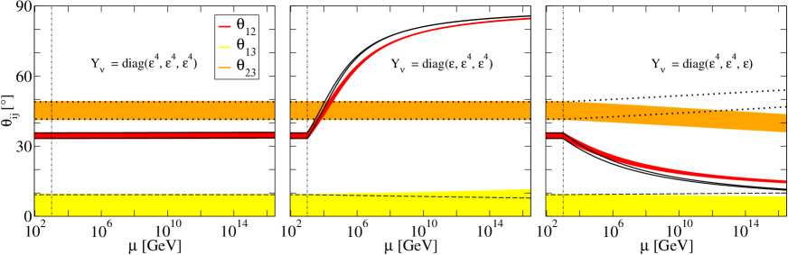
Figure 1: The RG evolution behavior of the three leptonic mixing angles as functions of the energy scale $\mu$ in the SM. We use $M_{0}=1~{}{\rm TeV}$ and $\varepsilon=0.3$ as input parameters at the seesaw scale. The colored regions correspond to values of the leptonic mixing angles within their 1$\sigma$ confidence intervals in the ND case, while the solid, dashed, and dotted curves denote the same confidence intervals in the ID case.

The left plot of Fig. 1 shows that, in the case of small Yukawa couplings, e.g. $|Y_{\nu}|\lesssim 0.01$, there is no visible RG running effects on the leptonic mixing angles both below and above the seesaw threshold. This can be observed from our analytical formulas, since in the limit $y_{i}\to 0$, $\dot{\theta}_{ij}\simeq 0$ hold for all the three leptonic mixing angles. Note that the meaning of $\varepsilon^{4}$ in the legends of Figs. 1-4 is that the corresponding element is basically negligible compared with elements that are indicated by $\varepsilon$. In the middle plot of Fig. 1, one of the Yukawa couplings in $Y_{\nu}$ is turned on, i.e., $y_{1}\simeq 0.3$, which leads to a significant increase of $\theta_{12}$ at the GUT scale. On the other hand, if $y_{1}$ is switched off, while $y_{2}$ or $y_{3}$ is turned on, as is shown in the right plot of Fig. 1, $\theta_{12}$ will decrease with increasing energy scale due to the opposite sign in front of $y_{1}$ and $y_{2}$ or $y_{3}$ in Eq. (23). From Fig. 1, we also find that the RG running of $\theta_{12}$ is qualitatively insensitive to the hierarchy of the masses of the light neutrinos. This is in agreement with our analytical results, since $\theta_{12}$ mainly receives corrections from $\zeta^{-1}_{21}$, which is positive for both possible hierarchies. Furthermore, there exist quasifixed points at $\pi/2$ or 0 in the RG running of $\theta_{12}$. Such a feature can be observed from Eq. (23), where $\dot{\theta}_{12}$ is proportional to both $s_{12}$ and $c_{12}$, which approaches zero when $\theta_{12}\sim 0$ or $\theta_{12}\sim\pi/2$. Finally, due to the lack of a sufficiently large enhancement factor, $\theta_{23}$ and $\theta_{13}$ are relatively stable against radiative corrections. In principle, a shift of a few degrees for $\theta_{23}$ can be achieved, see, for example, the right plot of Fig. 1. In the limit $y_{2}\simeq y_{3}$, their contributions to the RG running of $\theta_{23}$ and $\theta_{13}$ are canceled, which can also be seen from Eqs. (24) and (25).

In Fig. 2, we continue to illustrate the RG running of the leptonic mixing angles in the MSSM for both small and large values of $\tan\beta$.

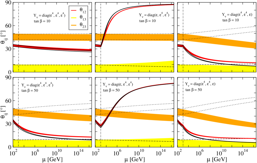
Figure 2: The RG evolution behavior of the three leptonic mixing angles as functions of the energy scale $\mu$ in the MSSM with $\tan\beta=10$ (upper plots) and $\tan\beta=50$ (lower plots), respectively. The input values of the masses of the heavy singlets and the Yukawa couplings are the same as those in Fig. 1.

Compared with the SM, the evolution of $\theta_{12}$ is analogous when the RG running is dominated by $Y_{\nu}$. For instance, in the middle and right columns of Fig. 2, $\theta_{12}$ approaches gradually its quasi-fixed points in both the small and large $\tan\beta$ cases. However, if $Y_{\nu}$ is suppressed, then the leading contributions to the RG running of $\theta_{12}$ originate from the charged-lepton Yukawa coupling $y_{\tau}$, in particular when $\tan\beta$ is sizable (see, for example, the left column of Fig. 2). This is similar to the RG evolution in the effective theory, where the charged-lepton corrections are enhanced by $\tan\beta$. Since $Y_{e}$ and $Y_{\nu}$ enter Eq. (23) with different signs, there is a cancellation between them, namely, the $Y_{\nu}$ contributions to the RG running are canceled somewhat by $Y_{e}$, and vice versa. In addition, the RG running of $\theta_{23}$ and $\theta_{13}$ may be modified by $y_{\tau}$, depending on the specific choice of the Yukawa couplings and the value of $\tan\beta$. From the lower-right plot in Fig. 2, one can observe that $\theta_{23}$ might acquire sizable corrections if $\tan\beta$ is large. In order for $\theta_{13}$ to have some visible RG running effects, arrangements of the CP-violating phases have to be incorporated, otherwise $\dot{\theta}_{13}\simeq 0$ according to Eq. (24). Therefore, the tiny RG running effects in Fig. 2 come from subleading order corrections.

The main difference between the RG running of the leptonic mixing angles in the SM and the MSSM is that the $y_{\tau}$ contributions to the running are negligible in the SM, while in the MSSM, they are amplified by $\tan\beta$. For example, in the case of $\tan\beta=50$, $y_{\tau}\simeq m_{\tau}/(v\cos\beta)\sim 0.3$, indicating a substantial modification of the RG running. In the case of $\tan\beta=10$, one can roughly estimate that $y_{\tau}\simeq m_{\tau}/(v\cos\beta)\sim 0.1$, which leads to a relatively small modification. This also reflects the fact that, in the MSSM, the RG running of the leptonic mixing angles in the case of a small $\tan\beta$ is weaker than that in the case of a large $\tan\beta$. In addition, the discrepancies between the RG running in the ND and ID cases originate from the sign changes in $\zeta^{-1}_{32}$ and $\zeta^{-1}_{31}$ as shown in Eqs. (24) and (25). For this reason, the RG running directions of $\theta_{23}$ and $\theta_{13}$ are changed if the mass hierarchy of the light neutrinos is reversed. Since the beta function of $\theta_{12}$ is primarily dominated by $\zeta^{-1}_{12}$, the running direction of $\theta_{12}$ is independent of the neutrino mass hierarchy, although the subleading order corrections may somewhat affect the RG running behavior.

V.2 Multiple thresholds

In the most general case with a nondegenerate mass spectrum of the heavy singlets, i.e., $M_{1}<M_{2}<M_{3}$, the RG running effects between the thresholds may modify the neutrino parameters remarkably in the SM. This case is called the multiple thresholds. In Fig. 3, we present the typical RG running behavior including three thresholds at 1, 10, and 100 TeV in the SM.

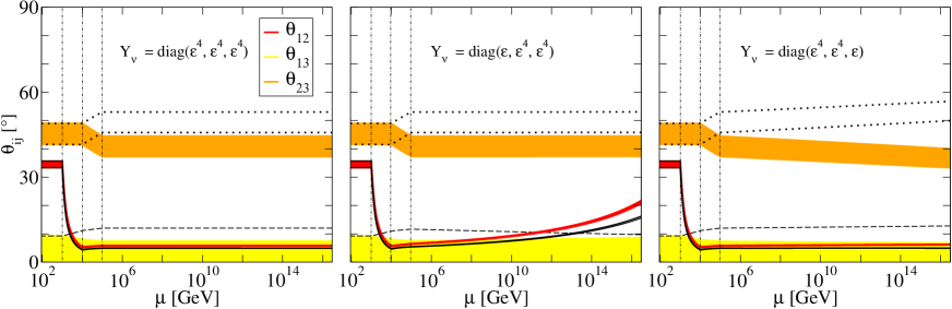
Figure 3: The RG evolution behavior of the three leptonic mixing angles as functions of the energy scale $\mu$ in the SM with the masses of the heavy neutrinos being $1$, $10$, and $100~{}{\rm TeV}$, respectively. The input values of the Yukawa couplings are the same as those in Fig. 1.

Note that the chosen values of the three thresholds serve as an order-of-magnitude example only. In crossing the thresholds from $M_{1}$ to $M_{3}$, $\theta_{12}$ is dramatically suppressed no matter the choice of $Y_{\nu}$. To identify the distinct threshold corrections, we return to Eq. (17), and observe that the neutrino mass matrix between the seesaw thresholds consists of two parts $\kappa$ and $Y_{\nu}M^{-1}_{\rm R}M_{S}(M^{T}_{\rm R})^{-1}Y^{T}_{\nu}$. In the SM, the beta functions of these two parts have different coefficients in the terms proportional to the gauge couplings and the Higgs self-coupling $\lambda$ Antusch et al. (2005). Therefore, keeping only the gauge coupling and $\lambda$ corrections in the corresponding beta functions, after a short-distance running from $M_{i}$ to $M_{i-1}$, the two parts of the neutrino mass matrix are rescaled to $a\kappa$ and $bY_{\nu}M^{-1}_{\rm R}M_{S}(M^{T}_{\rm R})^{-1}Y^{T}_{\nu}$, with $a\neq b$. Explicitly, we obtain the mass matrix of the light neutrinos at $\mu=M_{i-1}$ as

$$m_{\nu}\Big{|}_{M_{i-1}} \simeq bv^{2}\left[\kappa+Y_{\nu}M^{-1}_{\rm R}M_{S}(M^{T}_{\rm R})^{-1}Y^{T}_{\nu}\right]\Big{|}_{M_{i}}+(a-b)v^{2}\kappa\Big{|}_{M_{i}}$$ (33)

$$= bm_{\nu}\Big{|}_{M_{i}}+\Delta v^{2}\kappa\Big{|}_{M_{i}}\,,$$

where

$$\Delta\simeq\frac{1}{16\pi^{2}}\left(\frac{3}{2}g^{2}_{2}+\frac{9}{10}g^{2}_{1}+\lambda\right)\ln\left(\frac{M_{i-1}}{M_{i}}\right)\,.$$ (34)

One may treat the second term in Eq. (33) as a perturbation, arising from the RG running between the different thresholds. In contrast to the single threshold case, in which the RG corrections to the leptonic mixing angles are due to the large Yukawa couplings $Y_{e}$ and $Y_{\nu}$, the threshold corrections in this case are related to the gauge couplings and $\lambda$. Their nontrivial flavor structure is the reason for the observed RG running between the thresholds. Furthermore, if the masses of the light neutrinos are nearly degenerate, a short-distance running will result in sizable corrections to the corresponding leptonic mixing angle due to the enhancement factors $\zeta^{-1}_{ij}$.

The dramatic decrease of $\theta_{12}$ at around the first seesaw threshold observed in Fig. 3 is worth a further comment. First, the discontinuity of the beta function at the seesaw threshold is a direct consequence of the present renormalization scheme, in which the heavy singlets are decoupled abruptly. If one would instead use a mass-dependent scheme, the decoupling, and also the observed RG running, would be smooth. Although the values of the renormalized parameters in the vicinity of the thresholds are scheme dependent, the total amount of running is less so. Second, the negative slope of the curve between $M_{1}$ and $M_{2}$ is arguably an artifact of the diagonality assumption imposed on the neutrino Yukawa coupling matrix. This can clearly be observed from the discussion in Sec. V.4 and seen in the corresponding Fig. 7 where an opposite behavior is observed in the top-down approach with a nondiagonal Yukawa coupling matrix. Note that a similar discussion applies also to the RG running behavior of $\theta_{23}$ observed in Fig. 3.

Apart from the large variation at the seesaw thresholds, one may expect a further increase of $\theta_{12}$ between $M_{3}$ and the GUT scale (cf., the middle plot of Fig. 3), although it is very unlikely for the two large leptonic mixing angles $\theta_{23}$ and $\theta_{12}$ to unify at the GUT scale, unless one increases the values of the Yukawa couplings. On the other hand, a smaller $\theta_{12}$ could be favored at the GUT scale, in particular a Cabibbo-like angle, i.e., $\theta_{C}\sim 13^{\circ}$. In addition, $\theta_{23}$ acquires threshold corrections between the second and third thresholds. Although they are milder compared with that of $\theta_{12}$, the total amount of running between the thresholds can be large if $M_{3}/M_{2}$ is much larger than what it is in our example in Fig. 3.

In the MSSM, as we have shown in Sec. III, there is no mismatch between the RG running in the full and the effective theories. Therefore, the running behavior of all three leptonic mixing angles should be analogous to the ones in the single threshold case. The numerical results are presented in Fig. 4, which are in agreement with our expectations.

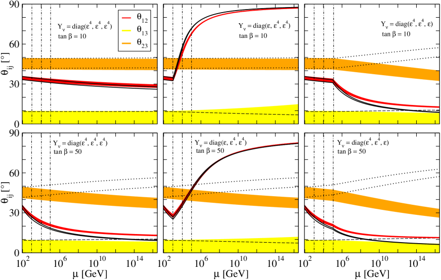
Figure 4: The RG evolution behavior of the three leptonic mixing angles as functions of the energy scale $\mu$ in the MSSM with the masses of the heavy neutrinos being $1$, $10$, and $100~{}{\rm TeV}$, respectively. Similar to Fig. 3, we use $\tan\beta=10$ for the upper plots and $\tan\beta=50$ for the lower plots. The input values of the Yukawa couplings are the same as those in Fig. 1.

In conclusion, the RG evolutions of the leptonic mixing angles between thresholds may lead to sizable corrections to the RG running in the SM, owing to vertex renormalization. In general, one should not simply use the matching condition at a common scale, unless the mass spectrum of the heavy singlets is considerably degenerate or the mass spectrum of the light neutrinos is very hierarchical (i.e., the NH or IH cases). Furthermore, we would like to comment on a phenomenologically meaningful situation, in which two of the masses of the heavy singlets are close to each other, while the other one is not, e.g., $M_{1}\simeq M_{2}<M_{3}$ or $M_{1}<M_{2}\simeq M_{3}$. In such scenarios, the threshold corrections to $\theta_{12}$ and $\theta_{13}$ are similar to those in the general three threshold scenario. However, in the latter case, $\theta_{23}$ is free of threshold effects, since it only receives visible threshold corrections in the RG running between $M_{2}$ and $M_{3}$, which can also be seen from Fig. 3.

V.3 Neutrino masses and CP-violating phases

For completeness, we perform the RG running of the neutrino masses and the CP-violating phases, despite the fact that there is still a lack of information on leptonic CP violation. As shown in Fig. 5 for the ND case, the RG running provides a common rescaling of the masses of the light neutrinos, and there is no sudden change along the running direction.

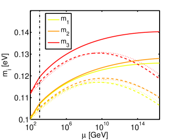
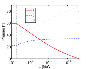
Figure 5: The RG evolution behavior of the masses of the light neutrinos (left plot) and the CP-violating phases (right plot) as functions of the energy scale $\mu$ in the ND case. We use $Y_{\nu}={\rm diag}(0.3,0.1,0.1)$ and $M_{0}=1~{}{\rm TeV}$ as an example. In the left plot, the solid, dashed, and dotted curves correspond to the cases of the SM, the MSSM with $\tan\beta=10$, and $\tan\beta=50$, respectively. In the right plot, we show the case of the SM only.

It can also be seen from Eqs. (29)-(31) that the RG running of the masses of the light neutrinos is mainly governed by the flavor blind part $\alpha_{\nu}$, while the $Y_{\nu}$ contributions are relatively small. There exits a maximal value of the masses of the light neutrinos in the MSSM at the energy scale $\mu\sim 10^{10}~{}{\rm GeV}$ due to the cancellation between gauge couplings and Yukawa couplings in $\alpha_{\nu}$, while such a local maximum does not appear in the SM. Note that similar RG running features of the masses of the light neutrinos also exist in the ID case.

In the single threshold case, the RG running of the CP-violating phases is also dominated by the corresponding Yukawa couplings. According to Eqs. (26)-(28), there are enhancement factors for both the Dirac and Majorana phases. Interestingly, even if one has a vanishing Dirac phase $\delta$ at a certain high-energy scale, a nonvanishing $\delta$ can be generated radiatively via the Majorana phases. This can be observed from the right plot of Fig. 5, where $\delta=0$ is obtained at the GUT scale. As we have pointed out, there is a subtlety at $\theta_{13}=0$, since the definition of $\delta$ loses its meaning. Hence, we choose $s_{13}=0.01$ in our realistic calculations. In addition, the Majorana phases $\rho$ and $\sigma$ run in the same direction, since the coefficients of their beta functions possess identical signs at leading order. A complete analysis of the RG running of the CP-violating phases could be interesting and useful for model building. However, such a study lies beyond the scope of this work.

V.4 Nondiagonal Yukawa couplings

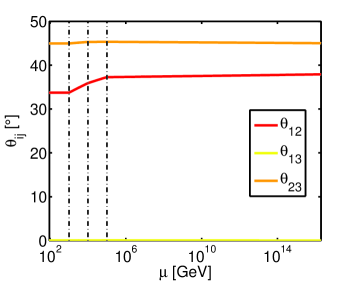
Figure 6: An example of the RG evolution of the leptonic mixing angles with a nondiagonal $Y_{\nu}$ in the SM. We focus on the NH case and use $m_{1}=0.01~{}{\rm eV}$ as a sample value.

Until now, our numerical analysis has been based on the assumption that both $Y_{e}$ and $Y_{\nu}$ are diagonal at the GUT scale. For the general case with arbitrary Yukawa couplings, it is very difficult to obtain analytical RGEs for the neutrino parameters due to the additional nonzero elements in $Y_{\nu}$. Thus, in this case, a top-down approach is highly favorable, despite the technical challenge of accommodating the low-energy data.

Not going into details, we focus on adding further support to the comments made in Sec. V.2 on the qualitative features of the behavior of $\theta_{12}$ and $\theta_{23}$ among the seesaw thresholds in the SM as depicted in Fig. 3. In Fig. 6, we show a numerical example corresponding to the NH case with an off-diagonal neutrino Yukawa coupling matrix of the form

$$Y_{\nu}=\left(\begin{matrix}\varepsilon^{4}&0&\varepsilon\cr 0&\varepsilon^{4}&0\cr\varepsilon&0&\varepsilon^{4}\end{matrix}\right)\,.$$ (35)

Unlike in the diagonal case of Fig. 3, one can find directly that $\theta_{12}$ increases across the seesaw thresholds and it can change significantly even between $M_{2}$ and $M_{3}$. Similarly, in Fig. 6, $\theta_{23}$ runs in the opposite direction compared with that in Fig. 3 and most of the running is experienced between $M_{1}$ and $M_{2}$. Note also that the magnitude of the effects in Fig. 6 is smaller than in Fig. 3, since a smaller value of $m_{1}$ is adopted for the sake of a better convergence of the top-down approach. Therefore, in Fig. 3, the sharp decline of $\theta_{12}$ is a consequence of the assumptions made on $Y_{\nu}$ rather than a generic feature.

V.5 Neutrino mixing patterns and flavor symmetries

While understanding the flavor puzzle is a fundamental task in particle physics, there are various flavor symmetric models constructed at high-energy scales, where the flavor symmetry is restored. In principle, any predictions from certain flavor symmetries encounter radiative corrections, and therefore, it is essential to take into account the RG running effects in determining physical parameters at an observable energy scale. In the effective theory, it is well known that the RG running effects are negligibly small in the SM. In the MSSM with nearly degenerate mass spectrum of the light neutrinos, $\theta_{12}$ decreases with increasing energy scale. In view of these features in the effective theory, there is no way to either unify $\theta_{12}$ and $\theta_{23}$ as suggested in the bimaximal mixing pattern ($s_{12}=s_{23}=1/\sqrt{2}$ and $s_{13}=0$ in the standard parametrization), or arrange them to the tri-bimaximal mixing pattern ($s_{12}=1/\sqrt{3}$, $s_{23}=1/\sqrt{2}$, and $s_{13}=0$ in the standard parametrization) at high-energy scales. Nevertheless, once the RG running effects above the seesaw scale are included, it makes sense to realize certain interesting mixing patterns at a unification scale. In Fig. 7, we illustrate the possibility of realizing the bimaximal and tri-bimaximal leptonic mixing patterns at the GUT scale via fine-tuning of the Yukawa couplings in the RGEs.

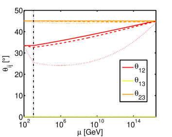
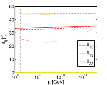
Figure 7: Realizations of the bimaximal (left plot) and the tri-bimaximal (right plot) neutrino mixing patterns at the GUT scale. Here we only consider the ND case. In addition, for simplicity, we use $M_{0}=1~{}{\rm TeV}$ for all the heavy singlets and take all the CP-violating phases to be zero. The solid, dashed, and dotted curves represent the SM, the MSSM with $\tan\beta=10$ and $\tan\beta=50$, respectively.

For simplicity, we only show the single seesaw threshold case. As examples, in the left plot of Fig. 7, we use

$$(y_{\nu 1},y_{\nu 2},y_{\nu 3})=(0.083,0.010,0.010),~{}(0.085,0.040,0.010),~{}(0.266,0.260,0.010)$$

in the SM, in the MSSM with $\tan\beta=10$, and in the MSSM with $\tan\beta=50$, respectively, whereas in the right plot of Fig. 7, we use

$$(y_{\nu 1},y_{\nu 2},y_{\nu 3})=(0.034,0.010,0.010),~{}(0.066,0.040,0.010),~{}(0.261,0.260,0.010)$$

in the SM, in the MSSM with $\tan\beta=10$, and in the MSSM with $\tan\beta=50$, respectively. In all cases, flavor symmetric mixing patterns are obtained according to the RG running. Thus various mixing patterns can be naturally achieved by adjusting the Yukawa couplings in the inverse seesaw model.

VI Comparison with other seesaw models

As discussed in Sec. I, there is no difference between the RG evolutions in low-scale effective theories. If we stick to the conventional type-I, -II, -III, and inverse seesaw models, at energy scales above the seesaw threshold, the RG running of the neutrino mass matrix can be uniformly described by

$$\dot{m}_{\nu}=N_{\nu}m_{\nu}+m_{\nu}N^{T}_{\nu}+\alpha_{\nu}m_{\nu}\,,$$ (36)

where

$$N_{\nu}=C_{e}Y_{e}Y^{\dagger}_{e}+C_{A}Y_{A}Y^{\dagger}_{A}\,,$$ (37)

with $Y_{A}$ being the Yukawa couplings between heavy seesaw particles and lepton doublets. The coefficients $\alpha_{\nu}$, $C_{e}$, and $C_{A}$ depend on the specific model. Apparently, sizable Yukawa couplings in Eq. (37) could give birth to visible RG running effects. In addition, threshold effects may induce significant corrections.

Let us now investigate these two points in detail. In the conventional type-I seesaw model, larger Yukawa couplings mean higher energy scale of the right-handed neutrinos, and thus, prominent RG running effects could emerge at some super-high-energy scale far above the scope of current experiments. If we lower the scale of the right-handed neutrinos by reducing the corresponding Yukawa couplings, threshold corrections may play an important role in the RG running. However, such a theory is still lacking testability, since the interactions between right-handed neutrinos and SM particles are suppressed by the Yukawa couplings, unless we use severe fine-tuning or specific assumptions on the model parameters Pilaftsis (1992); *Kersten:2007vk; *Antusch:2009gn; *Zhang:2009ac. In the type-II seesaw model, one may have sizable Yukawa couplings without facing the problem of lacking observability. However, as shown in Ref. Chao and Zhang (2007), there is no enhancement factor in the type-II seesaw framework, and one can hardly have visible RG running effects. For the simplest type-II seesaw model, there is only one triplet Higgs, which on the other hand prohibits the possibility of threshold corrections. The situation in the type-III seesaw model is similar to that in the type-I seesaw model, apart from the fact that, due to the charged components, there could be visible collider signatures no matter the magnitude of the Yukawa couplings.

The prominent feature of the RGEs in the inverse seesaw model is that significant RG running of the neutrino parameters could occur at lower energy scales without losing the testability at the current experiments. The RG running does not spoil the stability of the masses of the light neutrinos, but may introduce distinctive corrections to the lepton flavor structure. Indeed, this is related to the characteristic of the inverse seesaw model, namely, lepton number violation is well separated from lepton flavor violation.

Note that, in all cases with visible RG running effects, a nearly degenerate mass spectrum of the light neutrinos is required. Otherwise, there is no efficient enhancement factor boosting the running. Since the beta functions in Eqs. (29)-(31) are proportional to the masses of the light neutrinos explicitly, a nonvanishing mass cannot be generated via the RG running if it is zero at a certain energy scale.

VII Summary and conclusions

In this work, we have performed both analytical and numerical analyses of the RG running of the neutrino parameters in the inverse seesaw model. We have shown that, due to the sizable Yukawa couplings between light neutrinos and heavy gauge singlets in the inverse seesaw model, substantial RG running effects can be naturally obtained even at low-energy scales. Such a running distinguishes the inverse seesaw model from other simple seesaw models, and may be experimentally tested in near-future experiments. Concretely, we have derived very compact analytical RGEs for the neutrino parameters above the seesaw scale. Furthermore, a detailed numerical study of the RG running effects on the leptonic mixing angles has been carried out in both the SM and the MSSM. In general, we have found that there may be significant RG running effects on $\theta_{12}$ and $\theta_{23}$, and in particular on $\theta_{12}$, if the mass spectrum of the light neutrinos is nearly degenerate. Furthermore, the running between the seesaw thresholds corresponding to a certain hierarchy in the masses of the heavy neutrinos can be strong. The RG running effects of a nondiagonal Yukawa coupling matrix have also been briefly discussed. We have demonstrated that some phenomenologically and theoretically interesting leptonic mixing patterns, the bimaximal and tri-bimaximal patterns, can be achieved at a high-energy scale once the RG running effects are taken into account. In addition, the RG evolution of neutrino masses and CP-violating phases has been studied qualitatively. We have found that the Majorana phases run in the same direction and that a nonzero Dirac phase at low-energy scales can be generated from a vanishing one at some high-energy scale.

Appendix A Complete RGEs for neutrino parameters

The complete one-loop RG running of the masses of the light neutrinos are given by

$$\dot{m}_{1} = 2m_{1}\left\{c_{12}^{2}\left[s_{13}^{2}\left(s_{23}^{2}y_{2}^{2}+c_{23}^{2}y_{3}^{2}\right)+c_{13}^{2}y_{1}^{2}\right]+2s_{12}c_{12}s_{23}c_{23}s_{13}c_{\delta}\left(y_{2}^{2}-y_{3}^{2}\right)\right.$$ (38)

$$\left.+s_{12}^{2}\left(c_{23}^{2}y_{2}^{2}+s_{23}^{2}y_{3}^{2}\right)+\alpha_{\nu}\right\}\,,$$

$$\dot{m}_{2} = 2m_{2}\left[c_{12}^{2}\left(c_{23}^{2}y_{2}^{2}+s_{23}^{2}y_{3}^{2}\right)+2s_{12}c_{12}s_{23}c_{23}s_{13}c_{\delta}\left(y_{3}^{2}-y_{2}^{2}\right)+s_{12}^{2}c_{13}^{2}y_{1}^{2}\right.$$ (39)

$$\left.+s_{12}^{2}s_{13}^{2}\left(s_{23}^{2}y_{2}^{2}+c_{23}^{2}y_{3}^{2}\right)+\alpha_{\nu}\right]\,,$$

$$\dot{m}_{3} = 2m_{3}\left\{\left[c_{13}^{2}\left(s_{23}^{2}y_{2}^{2}+c_{23}^{2}y_{3}^{2}\right)+s_{13}^{2}y_{1}^{2}\right]+\alpha_{\nu}\right\}\,,$$ (40)

where we have defined $\dot{\theta}_{ij}\equiv 16\pi^{2}\mu\frac{{\rm d}\theta_{ij}}{{\rm d}\mu}$, $c_{\delta}\equiv\cos\delta$, $s_{\delta-\rho}\equiv\sin(\delta-\rho)$, and so on. Similarly, the full analytical results for the leptonic mixing angles and the Dirac CP-violating phase read

$$\dot{\theta}_{12} = \zeta_{21}s_{\rho-\sigma}\left\{s_{23}c_{23}s_{13}\left(2c_{\delta}s_{12}^{2}s_{\rho-\sigma}-s_{\delta+\rho-\sigma}\right)\left(y_{2}^{2}-y_{3}^{2}\right)\right.$$ (41)

$$\left.~{}~{}~{}+s_{12}c_{12}s_{\rho-\sigma}\left[c_{13}^{2}y_{1}^{2}+\left(s_{23}^{2}s_{13}^{2}-c_{23}^{2}\right)y_{2}^{2}-\left(s_{23}^{2}-c_{23}^{2}s_{13}^{2}\right)y_{3}^{2}\right]\right\}$$

$$+ \zeta_{31}s_{12}s_{13}s_{\delta+\rho}\left\{s_{12}s_{23}c_{23}s_{\rho}\left(y_{3}^{2}-y_{2}^{2}\right)+c_{12}s_{13}s_{\delta+\rho}\left[\left(y_{3}^{2}-y_{2}^{2}\right)s_{23}^{2}+y_{1}^{2}-y_{3}^{2}\right]\right\}$$

$$+ \zeta_{32}s_{13}s_{\delta+\sigma}\left\{s_{23}c_{23}s_{\sigma}\left(y_{3}^{2}-y_{2}^{2}\right)c_{12}^{2}-s_{12}c_{12}s_{13}s_{\delta+\sigma}\left[\left(y_{3}^{2}-y_{2}^{2}\right)s_{23}^{2}+y_{1}^{2}-y_{3}^{2}\right]\right\}$$

$$+ \frac{1}{\zeta_{21}}c_{\rho-\sigma}\left\{s_{23}c_{23}s_{13}\left(c_{\delta+\rho-\sigma}-2c_{\delta}c_{\rho-\sigma}s_{12}^{2}\right)\left(y_{3}^{2}-y_{2}^{2}\right)\right.$$

$$\left.~{}~{}~{}+s_{12}c_{12}c_{\rho-\sigma}\left[c_{13}^{2}y_{1}^{2}+\left(s_{23}^{2}s_{13}^{2}-c_{23}^{2}\right)y_{2}^{2}-\left(s_{23}^{2}-c_{23}^{2}s_{13}^{2}\right)y_{3}^{2}\right]\right\}$$

$$+ \frac{1}{\zeta_{31}}c_{\delta+\rho}s_{12}s_{13}\left\{s_{12}s_{23}c_{23}c_{\rho}\left(y_{3}^{2}-y_{2}^{2}\right)+c_{12}s_{13}c_{\delta+\rho}\left[\left(y_{3}^{2}-y_{2}^{2}\right)s_{23}^{2}+y_{1}^{2}-y_{3}^{2}\right]\right\}$$

$$+ \frac{1}{\zeta_{32}}c_{\delta+\sigma}s_{13}\left\{c_{12}^{2}s_{23}c_{23}c_{\sigma}\left(y_{3}^{2}-y_{2}^{2}\right)-s_{12}c_{12}s_{13}c_{\delta+\sigma}\left[\left(y_{3}^{2}-y_{2}^{2}\right)s_{23}^{2}+y_{1}^{2}-y_{3}^{2}\right]\right\}\,,$$

$$\dot{\theta}_{23} = \zeta_{31}s_{12}s_{\rho}\left\{c_{23}s_{12}s_{23}s_{\rho}\left(y_{2}^{2}-y_{3}^{2}\right)-c_{12}s_{13}s_{\delta+\rho}\left[\left(y_{3}^{2}-y_{2}^{2}\right)s_{23}^{2}+y_{1}^{2}-y_{3}^{2}\right]\right\}$$ (42)

$$+ \zeta_{32}s_{\sigma}\left\{c_{12}^{2}s_{23}c_{23}{}s_{\sigma}\left(y_{2}^{2}-y_{3}^{2}\right)+s_{12}c_{12}s_{13}s_{\delta+\sigma}\left[\left(y_{3}^{2}-y_{2}^{2}\right)s_{23}^{2}+y_{1}^{2}-y_{3}^{2}\right]\right\}$$

$$+ \frac{1}{\zeta_{31}}c_{\rho}s_{12}\left\{s_{12}s_{23}c_{23}c_{\rho}\left(y_{2}^{2}-y_{3}^{2}\right)-c_{12}s_{13}c_{\delta+\rho}\left[\left(y_{3}^{2}-y_{2}^{2}\right)s_{23}^{2}+y_{1}^{2}-y_{3}^{2}\right]\right\}$$

$$+ \frac{1}{\zeta_{32}}c_{\sigma}\left\{c_{12}^{2}s_{23}c_{23}c_{\sigma}\left(y_{2}^{2}-y_{3}^{2}\right)+s_{12}c_{12}s_{13}c_{\delta+\sigma}\left[\left(y_{3}^{2}-y_{2}^{2}\right)s_{23}^{2}+y_{1}^{2}-y_{3}^{2}\right]\right\}\,,$$

$$\dot{\theta}_{13} = \zeta_{31}c_{13}s_{\delta+\rho}\left\{c_{12}^{2}s_{13}s_{\delta+\rho}\left[\left(y_{3}^{2}-y_{2}^{2}\right)s_{23}^{2}+y_{1}^{2}-y_{3}^{2}\right]+s_{12}c_{12}s_{23}c_{23}s_{\rho}\left(y_{3}^{2}-y_{2}^{2}\right)\right\}$$ (43)

$$+ \zeta_{32}s_{12}c_{13}\text{ }s_{\delta+\sigma}\left\{c_{12}s_{23}c_{23}s_{\sigma}\left(y_{2}^{2}-y_{3}^{2}\right)+s_{12}s_{13}s_{\delta+\sigma}\left[\left(y_{3}^{2}-y_{2}^{2}\right)s_{23}^{2}+y_{1}^{2}-y_{3}^{2}\right]\right\}$$

$$+ \frac{1}{\zeta_{31}}c_{13}c_{\delta+\rho}\left\{c_{12}^{2}s_{13}c_{\delta+\rho}\left[\left(y_{3}^{2}-y_{2}^{2}\right)s_{23}^{2}+y_{1}^{2}-y_{3}^{2}\right]+s_{12}c_{12}s_{23}c_{23}c_{\rho}\left(y_{3}^{2}-y_{2}^{2}\right)\right\}$$

$$+ \frac{1}{\zeta_{32}}s_{12}c_{13}c_{\delta+\sigma}\left\{c_{12}s_{23}c_{23}c_{\sigma}\left(y_{2}^{2}-y_{3}^{2}\right)+s_{12}s_{13}c_{\delta+\sigma}\left[\left(y_{3}^{2}-y_{2}^{2}\right)s_{23}^{2}+y_{1}^{2}-y_{3}^{2}\right]\right\}\,,$$

$$\dot{\delta} = \frac{\zeta_{21}}{2c_{12}c_{23}s_{12}}\left\{2c_{\rho-\sigma}s_{13}s_{23}\left(s_{\delta+\rho-\sigma}-2c_{\delta}s_{12}^{2}s_{\rho-\sigma}\right)\left(y_{2}^{2}-y_{3}^{2}\right)c_{23}^{2}\right.$$ (44)

$$+\left.c_{12}s_{12}s_{2\rho-2\sigma}\left[-c_{13}^{2}y_{1}^{2}-\left(s_{13}^{2}s_{23}^{2}-c_{23}^{2}\right)y_{2}^{2}+\left(s_{23}^{2}-c_{12}^{2}s_{23}^{2}\right)y_{3}^{2}\right]c_{23}\right\}$$

$$+ \frac{\zeta_{31}}{2c_{12}c_{23}s_{13}s_{23}}\left\{c_{12}c_{23}s_{13}s_{23}\left[\left(\left(s_{23}^{2}\left(s_{2\delta+2\rho}s_{13}^{2}+2s_{2\rho}+s_{2\delta+2\rho}\right)-s_{2\rho}\right)y_{2}^{2}\right.\right.\right.$$

$$\left.+\left(s_{2\delta+2\rho}s_{13}^{2}+2c_{\delta}s_{\delta+2\rho}-s_{23}^{2}\left(s_{2\delta+2\rho}s_{13}^{2}+2s_{2\rho}+s_{2\delta+2\rho}\right)\right)y_{3}^{2}\right)s_{12}^{2}$$

$$-\left.\left(s_{12}^{2}\left(s_{13}^{2}+1\right)-1\right)s_{2\delta+2\rho}y_{1}^{2}-s_{2\delta+2\rho}\left(\left(y_{2}^{2}-y_{3}^{2}\right)s_{23}^{2}+y_{3}^{2}\right)\right]$$

$$+s_{12}\left[s_{13}^{2}\left(\left(4c_{\rho}s_{\delta+\rho}-s_{12}^{2}\left(s_{\delta}+3s_{\delta+2\rho}\right)\right)\left(y_{2}^{2}-y_{3}^{2}\right)s_{23}^{4}\right.\right.$$

$$+\left(\left(2s_{12}^{2}s_{\delta+2\rho}-2c_{\rho}s_{\delta+\rho}\right)y_{2}^{2}+2\left(3c_{\rho}s_{\delta+\rho}-s_{12}^{2}\left(s_{\delta}+2s_{\delta+2\rho}\right)\right)y_{3}^{2}\right)$$

$$\left.s_{23}^{2}-2c_{12}^{2}c_{\rho}\left(2s_{23}^{2}-1\right)s_{\delta+\rho}y_{1}^{2}-2c_{12}^{2}c_{\rho}s_{\delta+\rho}y_{3}^{2}\right)-\left.\left.2c_{12}^{2}c_{23}^{2}c_{\delta+\rho}s_{23}^{2}s_{\rho}\left(y_{2}^{2}-y_{3}^{2}\right)\right]\right\}$$

$$+ \frac{\zeta_{32}}{2c_{12}c_{23}s_{12}s_{13}s_{23}}\left\{c_{12}c_{23}s_{12}s_{13}s_{23}\left[\left(\left(2s_{2\sigma}+s_{2\delta+2\sigma}\right)\left(y_{3}^{2}-y_{2}^{2}\right)s_{23}^{2}+s_{2\sigma}\left(y_{2}^{2}-y_{3}^{2}\right)\right.\right.\right.$$

$$\left.+\left(s_{13}^{2}+1\right)s_{2\delta+2\sigma}y_{1}^{2}+s_{13}^{2}s_{2\delta+2\sigma}\left(y_{3}^{2}-y_{2}^{2}\right)s_{23}^{2}-s_{13}^{2}s_{2\delta+2\sigma}y_{3}^{2}-s_{2\delta+2\sigma}y_{3}^{2}\right)$$

$$\left.s_{12}^{2}+\left(2s_{23}^{2}-1\right)s_{2\sigma}\left(y_{2}^{2}-y_{3}^{2}\right)-s_{13}^{2}s_{2\delta+2\sigma}\left(\left(y_{3}^{2}-y_{2}^{2}\right)s_{23}^{2}+y_{1}^{2}-y_{3}^{2}\right)\right]$$

$$-c_{12}^{2}\left[\left(s_{13}^{2}\left(\left(s_{\delta}+3s_{\delta+2\sigma}\right)\left(y_{2}^{2}-y_{3}^{2}\right)s_{23}^{4}+\left(2\left(s_{\delta}+2s_{\delta+2\sigma}\right)y_{3}^{2}-2s_{\delta+2\sigma}y_{2}^{2}\right)s_{23}^{2}\right.\right.\right.$$

$$-\left.2c_{\sigma}\left(2s_{23}^{2}-1\right)s_{\delta+\sigma}y_{1}^{2}-2c_{\sigma}s_{\delta+\sigma}y_{3}^{2}\right)$$

$$\left.\left.\left.-2c_{23}^{2}c_{\delta+\sigma}s_{23}^{2}s_{\sigma}\left(y_{2}^{2}-y_{3}^{2}\right)\right)s_{12}^{2}+2c_{23}^{2}c_{\delta+\sigma}s_{13}^{2}s_{23}^{2}s_{\sigma}\left(y_{2}^{2}-y_{3}^{2}\right)\right]\right\}$$

$$+ \frac{1}{2c_{12}c_{23}s_{12}\zeta_{21}}\left\{-2\left(c_{\delta+\rho-\sigma}-2c_{\delta}c_{\rho-\sigma}s_{12}^{2}\right)s_{13}s_{23}s_{\rho-\sigma}\left(y_{2}^{2}-y_{3}^{2}\right)c_{23}^{2}\right.$$

$$-\left.c_{12}s_{12}s_{2\rho-2\sigma}\left[-c_{13}^{2}y_{1}^{2}-\left(s_{13}^{2}s_{23}^{2}-c_{23}^{2}\right)y_{2}^{2}+\left(s_{23}^{2}-c_{12}^{2}s_{23}^{2}\right)y_{3}^{2}\right]c_{23}\right\}$$

$$+ \frac{1}{2c_{12}c_{23}s_{13}s_{23}\zeta_{31}}\left\{c_{12}c_{23}s_{13}s_{23}\left[\left(-\left(2s_{2\rho}+s_{2\delta+2\rho}\right)\left(y_{2}^{2}-y_{3}^{2}\right)s_{23}^{2}\right.\right.\right.$$

$$\left.+s_{13}^{2}s_{2\delta+2\rho}\left(y_{3}^{2}-y_{2}^{2}\right)s_{23}^{2}+s_{2\rho}y_{2}^{2}-2c_{\delta}s_{\delta+2\rho}y_{3}^{2}-s_{13}^{2}s_{2\delta+2\rho}y_{3}^{2}\right)s_{12}^{2}$$

$$+\left.\left(s_{12}^{2}\left(s_{13}^{2}+1\right)-1\right)s_{2\delta+2\rho}y_{1}^{2}+s_{2\delta+2\rho}\left(\left(y_{2}^{2}-y_{3}^{2}\right)s_{23}^{2}+y_{3}^{2}\right)\right]$$

$$+s_{12}\left[\left(-\left(\left(s_{\delta}-3s_{\delta+2\rho}\right)s_{12}^{2}+4c_{\delta+\rho}s_{\rho}\right)\left(y_{2}^{2}-y_{3}^{2}\right)s_{23}^{4}\right.\right.$$

$$+\left(2\left(c_{\delta+\rho}s_{\rho}-s_{12}^{2}s_{\delta+2\rho}\right)y_{2}^{2}-2\left(\left(s_{\delta}-2s_{\delta+2\rho}\right)s_{12}^{2}+3c_{\delta+\rho}s_{\rho}\right)y_{3}^{2}\right)s_{23}^{2}$$

$$+\left.2c_{12}^{2}c_{\delta+\rho}\left(2s_{23}^{2}-1\right)s_{\rho}y_{1}^{2}+2c_{12}^{2}c_{\delta+\rho}s_{\rho}y_{3}^{2}\right)\left.\left.s_{13}^{2}+2c_{12}^{2}c_{23}^{2}c_{\rho}s_{23}^{2}s_{\delta+\rho}\left(y_{2}^{2}-y_{3}^{2}\right)\right]\right\}$$

$$+ \frac{1}{2c_{12}c_{23}s_{12}s_{13}s_{23}\zeta_{32}}\left\{\left[\left(s_{13}^{2}\left(-\left(s_{\delta}-3s_{\delta+2\sigma}\right)\left(y_{2}^{2}-y_{3}^{2}\right)s_{23}^{4}\right.\right.\right.\right.$$

$$-2\left(s_{\delta+2\sigma}y_{2}^{2}+\left(s_{\delta}-2s_{\delta+2\sigma}\right)y_{3}^{2}\right)s_{23}^{2}-\left.2c_{\delta+\sigma}\left(2s_{23}^{2}-1\right)s_{\sigma}y_{1}^{2}-2c_{\delta+\sigma}s_{\sigma}y_{3}^{2}\right)$$

$$-\left.\left.\left.2c_{23}^{2}c_{\sigma}s_{23}^{2}s_{\delta+\sigma}\left(y_{2}^{2}-y_{3}^{2}\right)\right)s_{12}^{2}+2c_{23}^{2}c_{\sigma}s_{13}^{2}s_{23}^{2}s_{\delta+\sigma}\left(y_{2}^{2}-y_{3}^{2}\right)\right)\right]c_{12}^{2}$$

$$+c_{23}s_{12}s_{13}s_{23}\left[\left(s_{13}^{2}s_{2\delta+2\sigma}\left(y_{2}^{2}-y_{3}^{2}\right)s_{23}^{2}+\left(2s_{2\sigma}+s_{2\delta+2\sigma}\right)\left(y_{2}^{2}-y_{3}^{2}\right)s_{23}^{2}\right.\right.$$

$$-\left.\left(s_{13}^{2}+1\right)s_{2\delta+2\sigma}y_{1}^{2}-s_{2\sigma}y_{2}^{2}+s_{2\sigma}y_{3}^{2}+s_{13}^{2}s_{2\delta+2\sigma}y_{3}^{2}+s_{2\delta+2\sigma}y_{3}^{2}\right)$$

$$\left.\left.s_{12}^{2}-\left(2s_{23}^{2}-1\right)s_{2\sigma}\left(y_{2}^{2}-y_{3}^{2}\right)+s_{13}^{2}s_{2\delta+2\sigma}\left(\left(y_{3}^{2}-y_{2}^{2}\right)s_{23}^{2}+y_{1}^{2}-y_{3}^{2}\right)\right]c_{12}\right\}\,.$$

In addition, the analytical RGEs for $\rho$ and $\sigma$ can be obtained by combining Eqs. (11), (19), and (20). However, the corresponding formulas are rather lengthy, and therefore, we do not list these tedious results here, since the evolution behavior is well described by Eqs. (26)-(28).

References

- Minkowski (1977) P. Minkowski, Phys. Lett. B67, 421 (1977)
- Yanagida (1979) T. Yanagida, in Proc. Workshop on the Baryon Number of the Universe and Unified Theories, edited by O. Sawada and A. Sugamoto (KEK, Tskuba, 1979), p. 95
- Gell-Mann et al. (1979) M. Gell-Mann, P. Ramond, and R. Slansky, in Supergravity, edited by P. van Nieuwenhuizen and D. Freedman (North Holland, Amsterdam, 1979), p. 315
- Mohapatra and Senjanović (1980) R. N. Mohapatra and G. Senjanović, Phys. Rev. Lett. 44, 912 (1980)
- Magg and Wetterich (1980) M. Magg and C. Wetterich, Phys. Lett. B94, 61 (1980)
- Schechter and Valle (1980) J. Schechter and J. W. F. Valle, Phys. Rev. D22, 2227 (1980)
- Wetterich (1981) C. Wetterich, Nucl. Phys. B187, 343 (1981)
- Lazarides et al. (1981) G. Lazarides, Q. Shafi, and C. Wetterich, Nucl. Phys. B181, 287 (1981)
- Mohapatra and Senjanović (1981) R. N. Mohapatra and G. Senjanović, Phys. Rev. D23, 165 (1981)
- Cheng and Li (1980) T. P. Cheng and L.-F. Li, Phys. Rev. D22, 2860 (1980)
- Foot et al. (1989) R. Foot, H. Lew, X. G. He, and G. C. Joshi, Z. Phys. C44, 441 (1989)
- Chankowski and Pluciennik (1993) P. H. Chankowski and Z. Pluciennik, Phys. Lett. B316, 312 (1993), eprint hep-ph/9306333
- Babu et al. (1993) K. S. Babu, C. N. Leung, and J. T. Pantaleone, Phys. Lett. B319, 191 (1993), eprint hep-ph/9309223
- Antusch et al. (2001) S. Antusch, M. Drees, J. Kersten, M. Lindner, and M. Ratz, Phys. Lett. B519, 238 (2001), eprint hep-ph/0108005
- Antusch et al. (2002a) S. Antusch, M. Drees, J. Kersten, M. Lindner, and M. Ratz, Phys. Lett. B525, 130 (2002a), eprint hep-ph/0110366
- Rossi (2002) A. Rossi, Phys. Rev. D66, 075003 (2002), eprint hep-ph/0207006
- Joaquim (2009) F. R. Joaquim (2009), eprint arXiv:0912.3427
- Chao and Zhang (2007) W. Chao and H. Zhang, Phys. Rev. D75, 033003 (2007), eprint hep-ph/0611323
- Schmidt (2007) M. A. Schmidt, Phys. Rev. D76, 073010 (2007), eprint arXiv:0705.3841
- Chakrabortty et al. (2009) J. Chakrabortty, A. Dighe, S. Goswami, and S. Ray, Nucl. Phys. B820, 116 (2009), eprint arXiv:0812.2776
- Pilaftsis (1992) A. Pilaftsis, Z. Phys. C55, 275 (1992), eprint hep-ph/9901206
- Kersten and Smirnov (2007) J. Kersten and A. Y. Smirnov, Phys. Rev. D76, 073005 (2007), eprint arXiv:0705.3221
- Antusch et al. (2010) S. Antusch, S. Blanchet, M. Blennow, and E. Fernández-Martínez, JHEP 01, 017 (2010), eprint arXiv:0910.5957
- Zhang and Zhou (2010) H. Zhang and S. Zhou, Phys. Lett. B685, 297 (2010), eprint arXiv:0912.2661
- Nath et al. (2009) P. Nath et al., Nucl. Phys. B, Proc. Suppl. 200-202, 180 (2010), eprint arXiv:1001.2693
- Mohapatra and Valle (1986) R. N. Mohapatra and J. W. F. Valle, Phys. Rev. D34, 1642 (1986)
- Bernabeu et al. (1987) J. Bernabeu, A. Santamaria, J. Vidal, A. Mendez, and J. W. F. Valle, Phys. Lett. B187, 303 (1987)
- Antusch et al. (2006) S. Antusch, C. Biggio, E. Fernández-Martínez, M. B. Gavela, and J. López-Pavón, JHEP 10, 084 (2006), eprint hep-ph/0607020
- Malinský et al. (2009) M. Malinský, T. Ohlsson, Z.-z. Xing, and H. Zhang, Phys. Lett. B679, 242 (2009), eprint arXiv:0905.2889
- Antusch et al. (2009a) S. Antusch, J. P. Baumann, and E. Fernández-Martínez, Nucl. Phys. B810, 369 (2009a), eprint arXiv:0807.1003
- Malinský et al. (2009) M. Malinský, T. Ohlsson, and H. Zhang, Phys. Rev. D79, 073009 (2009), eprint arXiv:0903.1961
- Fernández-Martínez et al. (2007) E. Fernández-Martínez, M. B. Gavela, J. López-Pavón, and O. Yasuda, Phys. Lett. B649, 427 (2007), eprint hep-ph/0703098
- Abada et al. (2007) A. Abada, C. Biggio, F. Bonnet, M. B. Gavela, and T. Hambye, JHEP 12, 061 (2007), eprint arXiv:0707.4058
- Xing (2008) Z.-z. Xing, Phys. Lett. B660, 515 (2008), eprint arXiv:0709.2220
- Goswami and Ota (2008) S. Goswami and T. Ota, Phys. Rev. D78, 033012 (2008), eprint arXiv:0802.1434
- Luo (2008) S. Luo, Phys. Rev. D78, 016006 (2008), eprint arXiv:0804.4897
- Altarelli and Meloni (2009) G. Altarelli and D. Meloni, Nucl. Phys. B809, 158 (2009), eprint arXiv:0809.1041
- Antusch et al. (2009b) S. Antusch, M. Blennow, E. Fernández-Martínez, and J. López-Pavón, Phys. Rev. D80, 033002 (2009b), eprint arXiv:0903.3986
- Rodejohann (2009) W. Rodejohann, Europhys. Lett. 88, 51001 (2009), eprint arXiv:0903.4590
- Antusch et al. (2005) S. Antusch, J. Kersten, M. Lindner, M. Ratz, and M. A. Schmidt, JHEP 03, 024 (2005), eprint hep-ph/0501272
- Mei (2005) J.-w. Mei, Phys. Rev. D71, 073012 (2005), eprint hep-ph/0502015
- Antusch et al. (2002b) S. Antusch, J. Kersten, M. Lindner, and M. Ratz, Phys. Lett. B538, 87 (2002b), eprint hep-ph/0203233
- Casas et al. (2000) J. A. Casas, J. R. Espinosa, A. Ibarra, and I. Navarro, Nucl. Phys. B573, 652 (2000), eprint hep-ph/9910420
- Chankowski et al. (2000) P. H. Chankowski, W. Krolikowski, and S. Pokorski, Phys. Lett. B473, 109 (2000), eprint hep-ph/9910231
- Antusch et al. (2003) S. Antusch, J. Kersten, M. Lindner, and M. Ratz, Nucl. Phys. B674, 401 (2003), eprint hep-ph/0305273
- Davidson and Ibarra (2001) S. Davidson and A. Ibarra, JHEP 09, 013 (2001), eprint hep-ph/0104076
- Joshipura (2002) A. S. Joshipura, Phys. Lett. B543, 276 (2002), eprint hep-ph/0205038
- Joshipura and Rindani (2003) A. S. Joshipura and S. D. Rindani, Phys. Rev. D67, 073009 (2003), eprint hep-ph/0211404
- Mei and Xing (2004) J.-w. Mei and Z.-z. Xing, Phys. Rev. D70, 053002 (2004), eprint hep-ph/0404081
- Dighe et al. (2009) A. Dighe, S. Goswami, and S. Ray, Phys. Rev. D79, 076006 (2009), eprint arXiv:0810.5680
- Schwetz et al. (2008) T. Schwetz, M. Tórtola, and J. W. F. Valle, New J. Phys. 10, 113011 (2008), eprint arXiv:0808.2016
- Xing et al. (2008) Z.-z. Xing, H. Zhang, and S. Zhou, Phys. Rev. D77, 113016 (2008), eprint arXiv:0712.1419
- Komatsu et al. (2010) E. Komatsu et al. (2010), eprint arXiv:1001.4538
- del Aguila et al. (2007) F. del Aguila, J. A. Aguilar-Saavedra, and R. Pittau, JHEP 10, 047 (2007), eprint hep-ph/0703261