Multiscale Analysis of Heterogeneous Media in the Peridynamic Formulation

Abstract

A methodology is presented for investigating the dynamics of heterogeneous media using the nonlocal continuum model given by the peridynamic formulation. The approach presented here provides the ability to model the macroscopic dynamics while at the same time resolving the dynamics at the length scales of the microstructure. Central to the methodology is a novel two-scale evolution equation. The rescaled solution of this equation is shown to provide a strong approximation to the actual deformation inside the peridynamic material. The two scale evolution can be split into a microscopic component tracking the dynamics at the length scale of the heterogeneities and a macroscopic component tracking the volume averaged (homogenized) dynamics. The interplay between the microscopic and macroscopic dynamics is given by a coupled system of evolution equations. The equations show that the forces generated by the homogenized deformation inside the medium are related to the homogenized deformation through a history dependent constitutive relation.

1 Introduction

The peridynamic formulation introduced in Silling [24] is a non-local continuum theory for deformable bodies. Material particles interact through a pairwise force field that acts within a prescribed horizon. Interactions depend only on the difference in the displacement of material points and spatial derivatives in the displacement are avoided. This feature makes it an attractive model for the autonomous evolution of discontinuities in the displacement for problems that involve cracks, interfaces, and other defects, see [2, 3, 15, 25, 26, 27]. Recent investigations aimed toward developing the numerical implementation, and application areas of the peridynamic model include [7], [30], [31], [32], [33]. More mathematically related investigations address issues related to the function space setting of peridynamics [12], [8] and the link between the linearized peridynamic formulation and the operators appearing in the Navier system of linear elasticity in the limit of vanishing non-locality [12], [29]. In this context the convergence of the solutions of the peridynamic equations to the solutions of the Navier system is demonstrated in [8]. In other related work the development of a non-local vector calculus with applications to non-local boundary value problems has been carried out in [16]. Recent work on the multi-scale applications of peridynamics have shown how the peridynamic equations formulated at mezo-scales can be recovered by a suitable upscaling of atomistic formulations, see [23].

In this paper new tools are developed for the analysis of heterogeneous peridynamic media involving two distinct length scales over which different types of peridynamic forces interact. The setting treated here involves a long range peridynamic force law perturbed in space by an oscillating short range peridynamic force. The oscillating short range force represents the presence of heterogeneities. It is also assumed that there is a sharp density variation associated with the heterogeneities. In this treatment we carry out the analysis in the small deformation setting. For this case the reference and deformed configurations are taken to be the same and both long and short range forces are given by linearizations of the peridynamic bond stretch model introduced in [24].

The relative length scale over which the short range forces interact is denoted by ${\varepsilon}$ and points inside the domain containing the heterogeneous material are specified by $x$. Here we will suppose the heterogeneities are periodically dispersed on the length scale ${\varepsilon}=\frac{1}{n}$ for some choice of $n=1,2,\ldots$ The deformation inside the medium is both a function of space and time $t$ and is written $u^{\varepsilon}(x,t)$. The multi-scale analysis of the peridynamic formulation proceeds using the concept of two-scale convergence, introduced and developed by Nguetseng [20] and subsequently in Allaire [1], see also E [9]. The two-scale convergence originally introduced in the context of partial differential equations turns out to provide a natural setting for identifying both the coarse scale and fine scale dynamics inside peridynamic composites. The theory and application of the two-scale convergence is taken up in section three of this paper where a novel two-scale peridynamic equation is derived. The two-scale formulation is described by introducing a rescaled or microscopic variable $y=x/{\varepsilon}$. The solution of the two-scale dynamics is a deformation $u(x,y,t)$ that depends on both variables $x$ and $y$.

The rescaled solution $u(x,x/{\varepsilon},t)$ is shown to provide a strong approximation to the actual deformation $u^{\varepsilon}(x,t)$ inside the peridynamic material. This is is shown in section 3.3 where an evolution law for the error $e^{\varepsilon}(x,t)=u^{\varepsilon}(x,t)-u(x,x/{\varepsilon},t)$ is developed. It is shown that $e^{\varepsilon}(x,t)$ vanishes in the $L^{p}$ norm, with respect to the spatial variables, when the length scale of the oscillation tends to zero for all $p$ in the interval $1\leq p\leq\infty$. The advantage of using the two-scale dynamics as a computational model is that it has the potential to lower computational costs associated with the explicit peridynamic modeling of millions of heterogeneities. This issue is discussed in section 3.3.

It is important for the modeling to recover the dynamics that can be measured by strain gages or other macroscopic measuring devices. Typical measured quantities involve averages of the deformation $u^{\varepsilon}(x,t)$ taken over a prescribed region $V$ with volume denoted by $|V|$. To this end we denote the unit period cell for the heterogeneities by $Y$ and project out the fluctuations by averaging over $y$ and write

$$u^{H}(x,t)=\int_{Y}u(x,y,t)dy.$$ (1.1)

In section four it is shown that

$$\lim_{{\varepsilon}\rightarrow 0}\frac{1}{|V|}\int_{V}u^{\varepsilon}(x,t)\,dx=\frac{1}{|V|}\int_{V}u^{H}(x,t)\,dx.$$ (1.2)

In this way we see that the average deformation is characterized by $u^{H}(x,t)$ when the scale ${\varepsilon}$ of the microstructure is small. We split the deformation into microscopic and macroscopic parts and write $u(x,y,t)=u^{H}(x,t)+r(x,y,t)$. The interplay between the microscopic and macroscopic dynamics is given by a coupled system of evolution equations for $u^{H}$ and $r$. The equations show that forces generated by the homogenized deformation inside the medium are related to the homogenized deformation through a history dependent constitutive relation. The explicit form of the constitutive relation is presented in section four where we present a homogenized evolution equation for the coarse scale dynamics written exclusively in terms of $u^{H}$, see (4.17).

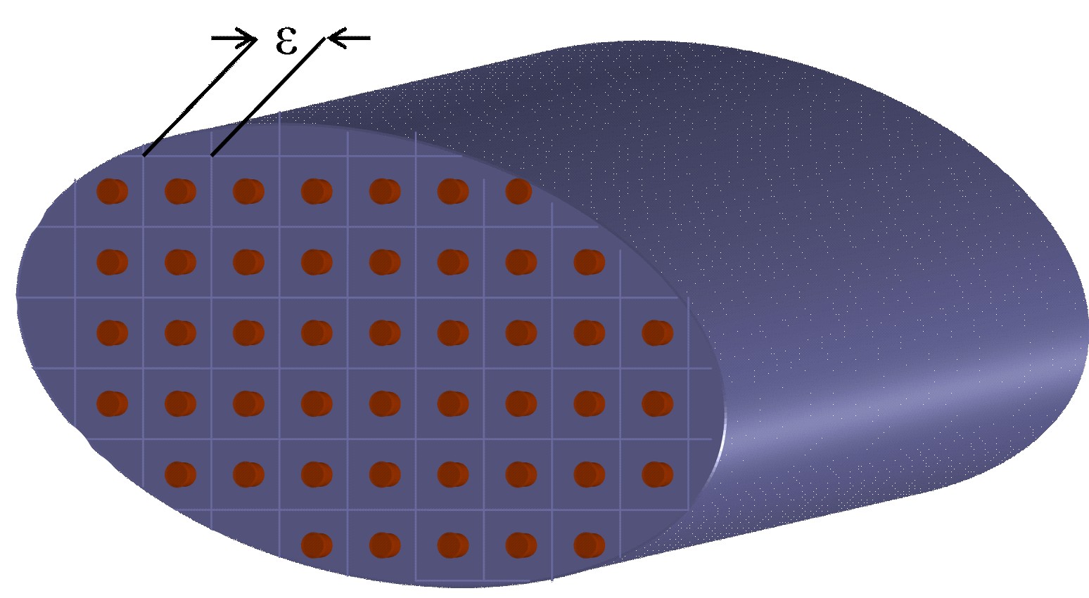
Figure 1: Fiber-reinforced composite.

1.1 Peridynamic Formulation of Continuum Mechanics in Heterogeneous Media

We consider elastic deformations inside a body described by the bounded domain $\Omega$. In the peridynamic theory, the time evolution of the displacement vector field $u$, in a homogeneous body of constant density $\hat{\rho}$ is given by the partial integro-differential equation

$$\hat{\rho}\;\partial_{t}^{2}u(x,t)=\int_{H_{\gamma}(x)\cap\Omega}f(u(\hat{x},t)-u(x,t),\hat{x}-x,x)\,d\hat{x}+b(u,x,t),\,\,\,\,\,\,(x,t)\in\Omega\times(0,T)$$ (1.3)

where $H_{\gamma}(x)$ is a neighborhood of $x$ of diameter $2\gamma$, $b$ is a prescribed loading force density field, and $\Omega$ is a bounded set in $\mathbb{R}^{3}$. Here $f$ denotes the pairwise force field whose value is the force vector (per unit volume squared) that the particle at $\hat{x}$ exerts on the particle at $x$. For a homogeneous medium $f$ is of the form $f(u(\hat{x},t)-u(x,t),\hat{x}-x)$, i.e., it depends only on the relative position of the two particles. We will often refer to $f$ as a bond force. Only points $\hat{x}$ inside $H_{\gamma}(x)$ interact with $x$. Equation (1.3) is supplemented with initial conditions for $u(x,0)$ and $\partial_{t}u(x,0)$. For the purposes of discussion it will be convenient to set

$$\xi=\hat{x}-x,$$

which represents the relative position of these two particles in the reference configuration, and

$$\eta=u(\hat{x},t)-u(x,t),$$

which represents their relative displacement (see Figure 2).

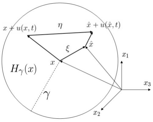
Figure 2: Deformation of a bond within the peridynamic horizon.

In this treatment, all elastic deformations are assumed small and the reference and deformed configurations are taken to be the same.

We now introduce the heterogeneous peridynamic material. One can think of it as a material with long range peridynamic forces acting over a neighborhood of diameter $2\gamma$ perturbed by an oscillating density fluctuation and oscillatory short range bond force acting over a much smaller neighborhood of diameter $2{\varepsilon}\delta$. Both the long and short range pairwise elastic forces will be given by the linearized version of the bond-stretch model proposed in [27]. The long range force is given by

$$f_{\mbox{{\scriptsize long}}}(\eta,\xi)=\left\{\begin{array}[]{c l}\displaystyle\lambda\frac{\xi\otimes\xi}{|\xi|^{3}}\eta,&|\xi|\leq\gamma\\ 0,&\mbox{otherwise}.\end{array}\right.$$

Here $\xi\otimes\xi$ is a rank one matrix with elements $(\xi\otimes\xi)_{ij}=\xi_{i}\xi_{j}$ and $\gamma$ is the prescribed peridynamic horizon and $\lambda$ is a positive constant.

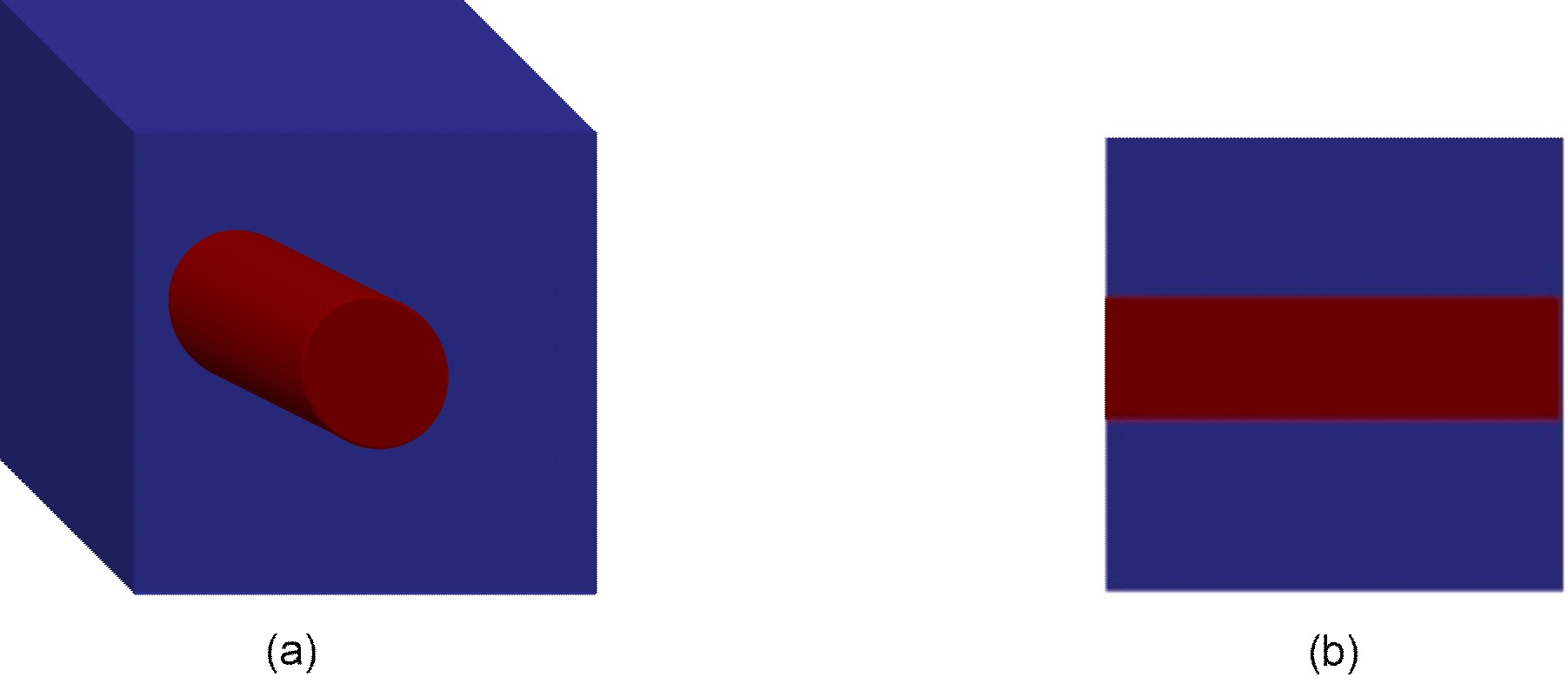
Figure 4: (a) Composite cube $Y$. (b) Cross-section of $Y$ along the fiber direction.

In this paper we assume that oscillations in the density and short range bond force are periodic. Here the oscillations are characterized by rescalings of a unit periodic peridynamic bond force and density. To describe these we introduce the unit period cube $Y\subset\mathbb{R}^{3}$ for the microstructure. The local coordinates inside $Y$ are denoted by $y$ with the origin at the center of the unit cube. The unit cube is composed of two or more peridynamic materials with different densities. To fix ideas one can consider reinforced composites made up of an inclusion phase such as a particle or fiber and a second host phase that surrounds the particle or fiber. A fiber reinforced material is portrayed in Figure 4. The presence of material heterogeneity is reflected by the appearance of peridynamic forces acting within the length scale of the period. Let $\chi_{\mbox{\scriptsize f}}$ denote the indicator function of the set occupied by the inclusion material and $\chi_{\mbox{\scriptsize m}}$ denote the the indicator function of the set occupied by the host or matrix material. Here $\chi_{\mbox{\scriptsize f}}$ is given by

$$\chi_{{\scriptsize\mbox{f}}}(y)=\left\{\begin{array}[]{c l}1,&$y$\mbox{ is in the inclusion phase},\\ 0,&\mbox{otherwise,}\end{array}\right.$$

and $\chi_{\mbox{\scriptsize m}}$ is given by

$$\chi_{\mbox{\scriptsize m}}(y)=1-\chi_{\mbox{\scriptsize f}}(y).$$

We extend the functions $\chi_{\mbox{\scriptsize f}}$ and $\chi_{\mbox{\scriptsize m}}$ to $\mathbb{R}^{3}$ by periodicity. For future reference, we denote by $\theta_{\mbox{\scriptsize f}}$ and $\theta_{\mbox{\scriptsize m}}$ the volume fractions of the included material and the matrix material, respectively. Here $\theta_{\mbox{\scriptsize f}}=\int_{Y}\chi_{\mbox{\scriptsize f}}(y)dy$ and $\theta_{\mbox{\scriptsize m}}=1-\theta_{\mbox{\scriptsize f}}$. The density of the matrix material inside the unit period cell is given by the unperturbed density $\rho_{\mbox{\scriptsize m}}=\hat{\rho}$ and that of the inclusion is given by $0<\rho_{\mbox{\scriptsize f}}=\hat{\rho}+\Delta\rho$ where $\Delta\rho$ can be a positive or negative constant. The density characterizing the heterogeneous medium is

$$\rho(y)=\chi_{\mbox{\scriptsize f}}(y)\rho_{\mbox{\scriptsize f}}+\chi_{\mbox{\scriptsize m}}(y)\rho_{\mbox{\scriptsize m}}.$$ (1.4)

The short-range pairwise force is characterized by a bond strength $\alpha_{\delta}$ associated with a horizon $\delta>0$. The peridynamic horizon $\delta$ is chosen to be smaller than the spacing separating the inclusions. In addition the inclusions are assumed to be sufficiently smooth so that the points $y$ and $\hat{y}$ are separated by at most one interface when $|y-\hat{y}|<\delta$. For any two points $y$ and $\hat{y}$ in $\mathbb{R}^{3}$ $\alpha_{\delta}$ is given by

$$\alpha_{\delta}(y,\hat{y})=\left\{\begin{array}[]{c l}C_{\mbox{{\scriptsize f}}},&\mbox{if $y$ and $\hat{y}$ are in the same inclusion and $|y-\hat{y}|<\delta$}\\ C_{\mbox{{\scriptsize m}}},&\mbox{if $y$ and $\hat{y}$ are in the matrix phase and $|y-\hat{y}|<\delta$}\\ C_{\mbox{{\scriptsize i}}},&\mbox{if $y$ and $\hat{y}$ are separated by an interface and $|y-\hat{y}|<\delta$}\\ 0,&\mbox{if $|y-\hat{y}|\geq\delta$}.\end{array}\right.$$

The material parameters $C_{\mbox{\scriptsize f}}$ and $C_{\mbox{\scriptsize m}}$ are intrinsic to each phase and can be determined through experiments. Bonds connecting particles in the different materials are characterized by $C_{\mbox{\scriptsize i}}$, which can be chosen such that $C_{\mbox{\scriptsize f}}>C_{\mbox{\scriptsize i}}>C_{\mbox{\scriptsize m}}>0$, see [27]. Mathematically we express the bond strength as

$$\alpha_{\delta}(y,\hat{y})=\chi_{\delta}(y-\hat{y})\alpha(y,\hat{y}),$$ (1.5)

where $\chi_{\delta}(z)=1$ for $|z|<\delta$ and $\chi_{\delta}(z)=0$ for $|z|\geq\delta$ and $\alpha$ is given by

$$\alpha(y,\hat{y})=C_{\mbox{\scriptsize f}}\;\chi_{\mbox{\scriptsize f}}(y)\chi_{\mbox{\scriptsize f}}(\hat{y})+C_{\mbox{\scriptsize m}}\;\chi_{\mbox{\scriptsize m}}(y)\chi_{\mbox{\scriptsize m}}(\hat{y})+C_{\mbox{\scriptsize i}}\left(\chi_{\mbox{\scriptsize f}}(y)\chi_{\mbox{\scriptsize m}}(\hat{y})+\chi_{\mbox{\scriptsize m}}(y)\chi_{\mbox{\scriptsize f}}(\hat{y})\right).$$ (1.6)

The short-range peridynamic force defined on $\Omega$ is given by

$$f_{\mbox{\scriptsize short}}^{{\varepsilon}}(\eta,\xi,x)=\frac{1}{{\varepsilon}^{2}}\,\alpha_{{\varepsilon}\delta}\left(\frac{x}{{\varepsilon}},\frac{x+\xi}{{\varepsilon}}\right)\;\frac{\xi\otimes\xi}{|\xi|^{3}}\eta.$$ (1.7)

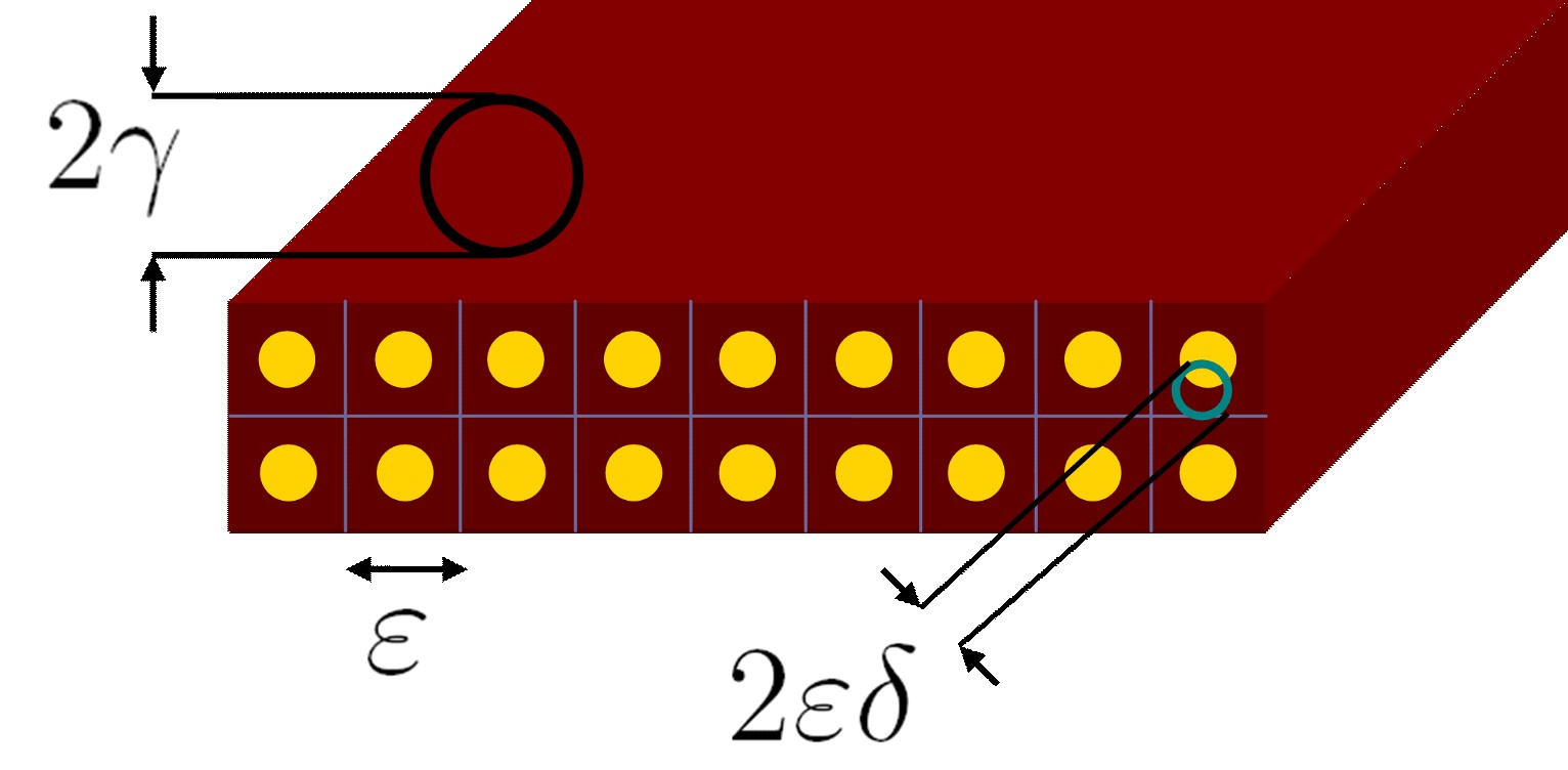
Figure 3: Long-range bonds (horizon $\gamma$) and short-range bonds (horizon ${\varepsilon}\delta$).

For future reference we see from (1.5) and (1.6) that $\alpha_{{\varepsilon}\delta}(\frac{x}{{\varepsilon}},\frac{\hat{x}}{{\varepsilon}})$ is given by

$$\alpha_{{\varepsilon}\delta}\left(\frac{x}{{\varepsilon}},\frac{\hat{x}}{{\varepsilon}}\right)=\chi_{{\varepsilon}\delta}(x-\hat{x})\left(C_{\mbox{\scriptsize f}}\;\chi^{{\varepsilon}}_{\mbox{\scriptsize f}}(x)\chi^{{\varepsilon}}_{\mbox{\scriptsize f}}(\hat{x})+C_{\mbox{\scriptsize m}}\;\chi^{{\varepsilon}}_{\mbox{\scriptsize m}}(x)\chi^{{\varepsilon}}_{\mbox{\scriptsize m}}(\hat{x})+C_{\mbox{\scriptsize i}}\left(\chi^{{\varepsilon}}_{\mbox{\scriptsize f}}(x)\chi^{{\varepsilon}}_{\mbox{\scriptsize m}}(\hat{x})+\chi^{{\varepsilon}}_{\mbox{\scriptsize m}}(x)\chi^{{\varepsilon}}_{\mbox{\scriptsize f}}(\hat{x})\right)\right),$$ (1.8)

where $\chi^{{\varepsilon}}_{\mbox{\scriptsize f}}(x):=\chi_{\mbox{\scriptsize f}}(\frac{x}{{\varepsilon}})$ and $\chi^{{\varepsilon}}_{\mbox{\scriptsize m}}(x):=\chi_{\mbox{\scriptsize m}}(\frac{x}{{\varepsilon}})$. The oscillating density $\rho_{\varepsilon}$ for the heterogeneous medium is given by $\rho_{\varepsilon}(x)=\rho(\frac{x}{{\varepsilon}})$.

The elastic displacement inside the heterogeneous body $\Omega$ is denoted by $u^{\varepsilon}(x,t)$ and the peridynamic equation of motion for the heterogeneous medium is given by

$$\begin{array}[]{lcl}\rho_{\varepsilon}(x)\partial_{t}^{2}u^{{\varepsilon}}(x,t)&=&\displaystyle\int_{H_{\gamma}(x)\cap\Omega}f_{\mbox{\scriptsize long}}(u^{{\varepsilon}}(\hat{x},t)-u^{{\varepsilon}}(x,t),\xi)\,d\hat{x}\\ &&\\ &&+\displaystyle\int_{H_{{\varepsilon}\delta}(x)\cap\Omega}f^{\varepsilon}_{\mbox{\scriptsize short}}((u^{{\varepsilon}}(\hat{x},t)-u^{{\varepsilon}}(x,t)),\xi,x)\,d\hat{x}\\ &&\\ &&+\displaystyle\,b^{\varepsilon}\left(x,t\right),\hbox{ for $x$ in $\Omega$.}\end{array}$$ (1.9)

The peridynamic equation is supplemented with initial conditions

$$u^{{\varepsilon}}(x,0) = u_{0}^{\varepsilon}(x)$$ (1.10)

$$\partial_{t}u^{{\varepsilon}}(x,0) = v_{0}^{\varepsilon}(x).$$ (1.11)

Here the body force $b^{\varepsilon}(x,t)$ and initial conditions $u_{0}^{\varepsilon}(x)$, $v_{0}^{\varepsilon}(x)$ can depend upon ${\varepsilon}$. When these functions are bounded in $L^{p}(\Omega)^{3}$ for $p\geq 1$ it follows from the theory of semigroups that there is a classic solution $u^{\varepsilon}(x,t)$ belonging to $C^{2}([0,T];\,L^{p}(\Omega)^{3})$. This is discussed in the following section, see Remark 2.2.

In what follows we will develop strong approximations for solutions $u^{\varepsilon}$ when the prescribed body forces and initial conditions are continuous at the coarse length scale but possess discontinuous oscillations over fine length scales. For this choice we look for a solution $u^{\varepsilon}(x,t)$ continuous in time but possibly discontinuous in the spacial variables and belonging to the Lebesgue space $L^{p}(\Omega)^{3}$ for $1\leq p<\infty$. In this paper we show that we can find solutions $u^{\varepsilon}(x,t)$ and strong approximations of the form $u(x,x/{\varepsilon},t)$ that both belong to $C^{2}([0,T];L^{p}(\Omega)^{3})$, for a wide class of initial conditions and body forces. In order to describe this class of initial conditions and body forces we consider the space $L^{p}_{\mbox{\scriptsize per}}(Y;C(\overline{\Omega})^{3})$ of functions $\psi(x,y)$ measurable with respect to $y$, $L^{p}$-integrable on $Y$ and $Y$-periodic in $y$, with values in the Banach space $C(\overline{\Omega})^{3}$ of continuous vector fields on $\overline{\Omega}$. Every element $\psi(x,y)$ of this space is a Caratheodory function and hence $\psi(x,\frac{x}{{\varepsilon}})$ is measurable on $\Omega$ and belongs to $L^{p}(\Omega)$. This kind of function space is well known in the context of two-scale convergence see, [1], and [21]. In what follows we will suppose $b(x,y,t)$ belongs to $C([0,T];\,L^{p}_{\mbox{\scriptsize per}}(Y;C(\overline{\Omega})^{3})$ and both $u_{0}(x,y)$ and $v_{0}(x,y)$ belong to $L^{p}_{\mbox{\scriptsize per}}(Y;C(\overline{\Omega})^{3})$. For this choice the initial conditions and body forces are given by $u^{\varepsilon}(x,0)=u_{0}(x,\frac{x}{{\varepsilon}})$, $\partial_{t}u^{{\varepsilon}}(x,0)=v_{0}(x,\frac{x}{{\varepsilon}})$, and $b^{\varepsilon}(x,t)=b(x,\frac{x}{{\varepsilon}},t)$. The construction of a strong approximation for this class of data is given in Theorem 3.12 of section 3.3.

It is important at this stage to point out that it is precisely the ${\varepsilon}^{-2}$ scaling of the bond force together with the scaling ${\varepsilon}\delta$ of the horizon that ultimately delivers the macroscopic equations for $u^{H}$ given by (4.17). In this context we expect other types of macroscopic equations to arise for different scalings of the bond force strength. Recent work for homogeneous media show that the classical equations of linear elasticity arise for bond force scaling on the order of ${\varepsilon}^{-4}$ and horizons with scaling ${\varepsilon}$, see [12], [29], and [8].

When the initial conditions and body force are continuous functions and the density $\rho^{\varepsilon}$ and bond forces characterized by $\alpha(\frac{x}{{\varepsilon}},\frac{\hat{x}}{{\varepsilon}})$ are also continuous then the solution $u^{\varepsilon}$ is continuous in space and belongs to $C^{2}([0,T];\,C(\overline{\Omega})^{3})$; this is discussed in the next section.

In forthcoming work we will focus on the development of strong approximations for initial conditions that are discontinuous with respect to coarse length scales. This will be carried out for heterogeneous peridynamic media characterized by oscillatory but continuous densities and bond forces. More generally one could contemplate strong approximations for more general combinations of bond forces and initial data.

2 Peridynamic Formulation for Heterogeneous Media: A Well Posed Problem

In this section, we make use of the semigroup theory of operators to show the existence and uniqueness of solutions to (1.9)-(1.11). For $v\in L^{p}(\Omega)^{3}$, with $1\leq p<\infty$, let

$$A^{\varepsilon}_{L,1}v(x) = \rho_{\varepsilon}^{-1}(x)\int_{H_{\gamma}(x)\cap\Omega}\lambda\frac{(\hat{x}-x)\otimes(\hat{x}-x)}{|\hat{x}-x|^{3}}\;v(\hat{x})\,d\hat{x},$$ (2.1)

$$A^{\varepsilon}_{L,2}v(x) = \rho_{\varepsilon}^{-1}(x)\int_{H_{\gamma}(x)\cap\Omega}\lambda\frac{(\hat{x}-x)\otimes(\hat{x}-x)}{|\hat{x}-x|^{3}}\,d\hat{x}\;v(x),$$ (2.2)

$$A^{{\varepsilon}}_{S,1}v(x) = \rho_{\varepsilon}^{-1}(x)\int_{H_{{\varepsilon}\delta}(x)\cap\Omega}\frac{1}{{\varepsilon}^{2}}\,\alpha\left(\frac{x}{{\varepsilon}},\frac{\hat{x}}{{\varepsilon}}\right)\frac{(\hat{x}-x)\otimes(\hat{x}-x)}{|\hat{x}-x|^{3}}\;v(\hat{x})\,d\hat{x},$$ (2.3)

$$A^{{\varepsilon}}_{S,2}v(x) = \rho_{\varepsilon}^{-1}(x)\int_{H_{{\varepsilon}\delta}(x)\cap\Omega}\frac{1}{{\varepsilon}^{2}}\,\alpha\left(\frac{x}{{\varepsilon}},\frac{\hat{x}}{{\varepsilon}}\right)\frac{(\hat{x}-x)\otimes(\hat{x}-x)}{|\hat{x}-x|^{3}}\,d\hat{x}\;v(x).$$ (2.4)

Also we set

$$A^{\varepsilon}_{L} = A^{\varepsilon}_{L,1}-A^{\varepsilon}_{L,2},$$ (2.5)

$$A^{{\varepsilon}}_{S} = A^{{\varepsilon}}_{S,1}-A^{{\varepsilon}}_{S,2},$$ (2.6)

$$A^{{\varepsilon}} = A^{\varepsilon}_{L}+A^{{\varepsilon}}_{S}.$$ (2.7)

Then by making the identifications $u^{{\varepsilon}}(t)=u^{{\varepsilon}}(\cdot,t)$ and $b^{{\varepsilon}}(t)=b(\cdot,t)$, we can write (1.9)-(1.11) as an operator equation in $L^{p}(\Omega)^{3}$

$$\left\{\begin{array}[]{ccl}\ddot{u}^{{\varepsilon}}(t)&=&A^{{\varepsilon}}u^{{\varepsilon}}(t)+\rho_{\varepsilon}^{-1}b^{{\varepsilon}}(t),\;\;\;\;\;t\in[0,T]\\ u^{{\varepsilon}}(0)&=&u^{{\varepsilon}}_{0},\\ \dot{u}^{{\varepsilon}}(0)&=&v^{{\varepsilon}}_{0}.\end{array}\right.$$ (2.8)

or equivalently, as an inhomogeneous Abstract Cauchy Problem in
$L^{p}(\Omega)^{3}\times L^{p}(\Omega)^{3}$

$$\left\{\begin{array}[]{ccl}\dot{U}^{{\varepsilon}}(t)&=&\mathbb{A}^{{\varepsilon}}U^{{\varepsilon}}(t)+B^{{\varepsilon}}(t),\;\;\;\;\;t\in[0,T]\\ U^{{\varepsilon}}(0)&=&U^{{\varepsilon}}_{0}.\\ \end{array}\right.$$ (2.9)

where

$$U^{{\varepsilon}}(t)=\left(\begin{array}[]{c}u^{{\varepsilon}}(t)\\ \dot{u}^{{\varepsilon}}(t)\\ \end{array}\right),\,\,U^{{\varepsilon}}_{0}=\left(\begin{array}[]{c}u^{{\varepsilon}}_{0}\\ v^{{\varepsilon}}_{0}\\ \end{array}\right),\,\,B^{{\varepsilon}}(t)=\left(\begin{array}[]{c}0\\ \rho_{\varepsilon}^{-1}b^{{\varepsilon}}(t)\\ \end{array}\right),\mbox{ and }\mathbb{A}^{{\varepsilon}}=\left(\begin{array}[]{cc}0&I\\ A^{{\varepsilon}}&0\\ \end{array}\right).$$

Here $I$ denotes the identity map in $L^{p}(\Omega)^{3}$.

Proposition 2.1.

Let $1\leq p<\infty$ and assume that $b\in C([0,T];\,L^{p}_{\mbox{\scriptsize per}}(Y;C(\overline{\Omega})^{3}))$ and $U_{0}\in L^{p}_{\mbox{\scriptsize per}}(Y;C(\overline{\Omega})^{3})\times L^{p}_{\mbox{\scriptsize per}}(Y;C(\overline{\Omega})^{3})$. Then

1. The operators $A^{{\varepsilon}}$ and $\mathbb{A}^{{\varepsilon}}$ are linear and bounded on $L^{p}(\Omega)^{3}$ and $L^{p}(\Omega)^{3}\times L^{p}(\Omega)^{3}$, respectively. Moreover, the bounds are uniform in ${\varepsilon}$.

2. Equation (2.9) has a unique classical solution $U^{{\varepsilon}}$ in $C^{1}([0,T];\,L^{p}(\Omega)^{3}\times L^{p}(\Omega)^{3})$ which is given by

   $$U^{{\varepsilon}}(t)=e^{t\mathbb{A}^{{\varepsilon}}}U^{{\varepsilon}}_{0}+\int_{0}^{t}e^{(t-\tau)\mathbb{A}^{{\varepsilon}}}B^{{\varepsilon}}(\tau)\,d\tau,\,\,\,t\in[0,T],$$ (2.11)

   where

   $$e^{t\mathbb{A}^{{\varepsilon}}}=\sum_{n=0}^{\infty}\frac{t^{n}}{n!}\;(\mathbb{A}^{{\varepsilon}})^{n}.$$ (2.12)

   Moreover, equation (2.8) has a unique classical solution $u^{{\varepsilon}}\in C^{2}([0,T];\,L^{p}(\Omega)^{3})$ which is given by

   $$u^{{\varepsilon}}(t) = \cosh{\left(t\sqrt{A^{{\varepsilon}}}\right)}u^{{\varepsilon}}_{0}+\sqrt{A^{{\varepsilon}}}^{\;-1}\sinh{\left(t\sqrt{A^{{\varepsilon}}}\right)}v^{{\varepsilon}}_{0}$$ (2.13a)

   $$+\sqrt{A^{{\varepsilon}}}^{\;-1}\!\int_{0}^{t}\sinh{\left((t-\tau)\sqrt{A^{{\varepsilon}}}\right)}b^{{\varepsilon}}(\tau)\,d\tau$$

   with the notation

   $$\cosh{\left(t\sqrt{A^{{\varepsilon}}}\right)}:=\sum_{n=0}^{\infty}\frac{t^{2n}}{(2n)!}\;(A^{{\varepsilon}})^{n}$$ (2.13b)

   $$\sqrt{A^{{\varepsilon}}}^{\;-1}\sinh{\left(t\sqrt{A^{{\varepsilon}}}\right)}:=\sum_{n=0}^{\infty}\frac{t^{2n+1}}{(2n+1)!}\;(A^{{\varepsilon}})^{n}$$ (2.13c)

3. The sequences $(u^{{\varepsilon}})_{{\varepsilon}>0}$, $(\dot{u}^{{\varepsilon}})_{{\varepsilon}>0}$, and $(\ddot{u}^{{\varepsilon}})_{{\varepsilon}>0}$ are bounded in $L^{\infty}([0,T];\,L^{p}(\Omega)^{3})$.

Remark 2.2.

The hypothesis of Proposition 2.1 can be relaxed by assuming that the sequences of initial conditions $\left(u_{0}^{{\varepsilon}}\right),\left(v_{0}^{{\varepsilon}}\right)$, are bounded in $L^{p}(\Omega)^{3}$ and $\left(b^{{\varepsilon}}(\cdot,t)\right)$ is uniformly bounded in $L^{p}(\Omega)^{3}$ for $t\in[0,T]$. This is proved following the same steps given in the proof of Proposition 2.1 presented below.

Proof.

Part (a). It is clear that the operators $A^{{\varepsilon}}_{S,1}$, $A^{{\varepsilon}}_{S,2}$, $A^{{\varepsilon}}_{L,1}$, and $A^{{\varepsilon}}_{L,2}$ are linear. So we begin the proof by showing that $A^{{\varepsilon}}_{S,1}$ and $A^{{\varepsilon}}_{S,2}$ are uniformly bounded sequences of operators on $L^{p}(\Omega)^{3}$ for $1\leq p<\infty$. We introduce the indicator function $\chi_{\scriptscriptstyle{\Omega}}(x)$ taking the value one for $x$ inside $\Omega$ and zero for $x$ outside $\Omega$ and let $v$ denote a generic vector field belonging to $L^{p}(\Omega)^{3}$. Then by the change of variables $\hat{x}=x+{\varepsilon}z$ in (2.3) we obtain

$$A^{{\varepsilon}}_{S,1}v(x) = \rho_{\varepsilon}^{-1}\int_{H_{\delta}(0)}\chi_{\scriptscriptstyle{\Omega}}(x+{\varepsilon}z)\alpha\left(\frac{x}{{\varepsilon}},\frac{x}{{\varepsilon}}+z\right)\frac{z\otimes z}{|z|^{3}}\;v(x+{\varepsilon}z)\,dz.$$ (2.14)

Applying Minkowski’s inequality gives

$$\|A^{{\varepsilon}}_{S,1}v(x)\|_{L^{p}(\Omega)^{3}}\leq\int_{H_{\delta}(0)}\left(\int_{\Omega}\chi_{\scriptscriptstyle{\Omega}}(x+{\varepsilon}z)\rho^{-1}(\frac{x}{{\varepsilon}})|\alpha\left(\frac{x}{{\varepsilon}},\frac{x}{{\varepsilon}}+z\right)\frac{z\otimes z}{|z|^{3}}\;v(x+{\varepsilon}z)|^{p}\,dx\right)^{1/p}\,dz.$$ (2.15)

Let $\displaystyle\overline{\alpha}=\max_{y,y^{\prime}\in Y}\rho^{-1}(y)\alpha(y,y^{\prime})$ and we see that

$$\|A^{{\varepsilon}}_{S,1}v(x)\|_{L^{p}(\Omega)^{3}} \leq \overline{\alpha}\int_{H_{\delta}(0)}\frac{1}{|z|}\;\left(\int_{\Omega}\chi_{\scriptscriptstyle{\Omega}}(x+{\varepsilon}z)|v(x+{\varepsilon}z)|^{p}\,dx\right)^{1/p}\,dz$$ (2.16)

$$\leq M_{S}\|v\|_{L^{p}(\Omega)^{3}},$$

where $M_{S}$ is independent of ${\varepsilon}$ and given by

$$M_{S}=\overline{\alpha}\;\left(\int_{H_{\delta}(0)}\frac{1}{|z|}\,dz\right)=\overline{\alpha}\frac{2\pi\delta^{2}}{3},$$ (2.17)

which shows that the operators are $A^{{\varepsilon}}_{S,1}$ is uniformly bounded with respect to ${\varepsilon}$. Similarly, $A^{{\varepsilon}}_{S,2}$ can be written as

$$A^{{\varepsilon}}_{S,2}v(x) = \int_{H_{\delta}(0)}\chi_{\scriptscriptstyle{\Omega}}(x+{\varepsilon}z)\rho^{-1}(\frac{x}{{\varepsilon}})\alpha\left(\frac{x}{{\varepsilon}},\frac{x}{{\varepsilon}}+z\right)\frac{z\otimes z}{|z|^{3}}\,dz\,\;v(x).$$ (2.18)

Thus

$$|A^{{\varepsilon}}_{S,2}v(x)| \leq M_{S}\;|v(x)|,$$

from which the boundedness of $A^{{\varepsilon}}_{S,2}$ immediately follows. Combining these results shows that $A_{S}^{{\varepsilon}}$, which is given by $A^{{\varepsilon}}_{S,1}-A^{{\varepsilon}}_{S,2}$, is a sequence of uniformly bounded operators on $L^{p}(\Omega)^{3}$.

Next we show that the linear operators $A_{L}^{\varepsilon}=A^{{\varepsilon}}_{L,1}-A^{{\varepsilon}}_{L,2}$ are a sequence of uniformly bounded operators on $L^{p}(\Omega)^{3}$. Changing variables $\hat{x}=x+\xi$ and applying Minkowski’s inequality gives

$$\|\,A^{{\varepsilon}}_{L,1}v\,\|_{L^{p}(\Omega)^{3}} \leq \int_{H_{\gamma}(0)}\left(\int_{\Omega}\chi_{\scriptscriptstyle{\Omega}}(x+\xi)\rho^{-1}(\frac{x}{{\varepsilon}})|\lambda\frac{\xi\otimes\xi}{|\xi|^{3}}\;v(x+\xi)|^{p}\,dx\right)^{1/p}\,d\xi$$ (2.19)

$$\leq M_{L}\|\,v\,\|_{L^{p}(\Omega)^{3}}$$

where $M_{L}$ is given by

$$M_{L}=\max_{y\in Y}\{\rho^{-1}(y)\}\times\lambda\frac{2\pi\gamma^{2}}{3},$$ (2.20)

and it follows that the operator $A^{{\varepsilon}}_{L,1}$ is bounded in $L^{p}(\Omega)^{3}$. The boundedness of $A^{{\varepsilon}}_{L,2}$, which is given by (2.2), follows immediately from its definition. Therefore $A^{{\varepsilon}}_{L}$ is uniformly bounded on $L^{p}(\Omega)^{3}$ with respect to ${\varepsilon}$.

Since $A^{{\varepsilon}}=A^{{\varepsilon}}_{L}+A^{{\varepsilon}}_{S}$, we conclude that

$$\|A^{{\varepsilon}}v\|_{L^{p}(\Omega)^{3}}\leq M\,\|v\|_{L^{p}(\Omega)^{3}},$$ (2.21)

for a positive constant $M$ which is independent of ${\varepsilon}$. The operator $\mathbb{A}^{{\varepsilon}}$ is clearly linear, thus it remains to show that this operator is uniformly bounded on $L^{p}(\Omega)^{3}\times L^{p}(\Omega)^{3}$. To see this, we let $(v,w)\in L^{p}(\Omega)^{3}\times L^{p}(\Omega)^{3}$. The norm in this Banach space is given by

$$\|(v,w)\|_{L^{p}(\Omega)^{3}\times L^{p}(\Omega)^{3}}=\|v\|_{L^{p}(\Omega)^{3}}+\|w\|_{L^{p}(\Omega)^{3}}.$$

We note that

$$\mathbb{A}^{{\varepsilon}}{\small\left(\begin{array}[]{c}v\\ w\\ \end{array}\right)=\left(\begin{array}[]{cc}0&I\\ A^{{\varepsilon}}&0\\ \end{array}\right)\left(\begin{array}[]{c}v\\ w\\ \end{array}\right)=\left(\begin{array}[]{c}w\\ A^{{\varepsilon}}v\\ \end{array}\right).}$$

Thus we obtain

$$\|\mathbb{A}^{{\varepsilon}}(v,w)\|_{L^{p}(\Omega)^{3}\times L^{p}(\Omega)^{3}} = \|w\|_{L^{p}(\Omega)^{3}}+\|A^{{\varepsilon}}v\|_{L^{p}(\Omega)^{3}}$$ (2.23)

$$\leq \|w\|_{L^{p}(\Omega)^{3}}+\|A^{{\varepsilon}}\|\,\|v\|_{L^{p}(\Omega)^{3}}.$$

From (2.23) it follows that

$$\|\mathbb{A}^{{\varepsilon}}(v,w)\|_{L^{p}(\Omega)^{3}\times L^{p}(\Omega)^{3}}\leq M\|(v,w)\|_{L^{p}(\Omega)^{3}\times L^{p}(\Omega)^{3}},$$ (2.24)

for some positive constant $M$ completing the argument.

Part (b). We have seen from Part (a) that $\mathbb{A}^{{\varepsilon}}$ is a bounded linear operator on the Banach space $L^{p}(\Omega)^{3}\times L^{p}(\Omega)^{3}$. Also, since $b^{{\varepsilon}}$ is in $C([0,T];\,L^{p}(\Omega)^{3})$, it follows that $B^{{\varepsilon}}=(0,b^{{\varepsilon}})$ is in $C([0,T];\,L^{p}(\Omega)^{3}\times L^{p}(\Omega)^{3})$. From these facts, it follows from the theory of semigroups, see for example, [22, 13].

1. The operator $\mathbb{A}^{{\varepsilon}}$ generates a uniformly continuous semigroup $\{e^{t\mathbb{A}^{{\varepsilon}}}\}_{t\geq 0}$ on $L^{p}(\Omega)^{3}\times L^{p}(\Omega)^{3}$, where $e^{t\mathbb{A}^{{\varepsilon}}}$ is given by (2.12).

2. The inhomogeneous Abstract Cauchy Problem (2.9) has a unique classical solution $U^{{\varepsilon}}\in C^{1}([0,T];\,L^{p}(\Omega)^{3}\times L^{p}(\Omega)^{3})$ which is given by (2.11).

It immediately follows from (2) that the second order inhomogeneous Abstract Cauchy Problem (2.8) has a unique classical solution $u^{{\varepsilon}}\in C^{2}([0,T];\,L^{p}(\Omega)^{3})$ and formula (2.13) follows immediately from (2.12).

Part (c). We recall that

$$u^{{\varepsilon}}_{0}(x) := u_{0}(x,\frac{x}{{\varepsilon}})$$

$$v^{{\varepsilon}}_{0}(x) := v_{0}(x,\frac{x}{{\varepsilon}})$$

where $u_{0}(x,y)$, $v_{0}(x,y)$ are in $L^{p}_{\mbox{\scriptsize per}}(Y;C(\overline{\Omega})^{3})$. We surround $\Omega$ by a cube of integer side length $L$ and extend $u_{0}(x,y)$ to the cube by setting $u_{0}(x,y)=0$ for $x$ outside $\Omega$ and for every $y$ in $Y$. We note that the extended $u_{0}(x,\frac{x}{{\varepsilon}})$ is ${\varepsilon}=\frac{1}{n}$ periodic in the second variable and shift the cube so that it is commensurate with the periods. The period cells of side length ${\varepsilon}$ are denoted by ${\varepsilon}Y_{i}$ and the cube is given by their union $\cup_{i}{\varepsilon}Y_{i}$ where the index $i$ ranges from $1$ to $L^{3}n^{3}$. Since we have extended $u_{0}(x,y)$ so that it vanishes when $x$ lies outside $\Omega$ one can write

$$\|u^{{\varepsilon}}_{0}\|_{L^{p}(\Omega)^{3}} = \left(\int_{\cup_{i}{\varepsilon}Y_{i}}|u_{0}(x,\frac{x}{{\varepsilon}})|^{p}\,dx\right)^{1/p}.$$ (2.25)

Hence

$$\|u^{{\varepsilon}}_{0}\|_{L^{p}(\Omega)^{3}} \leq \left(\int_{\cup_{i}{\varepsilon}Y_{i}}\sup_{x^{\prime}\in\Omega}|u_{0}(x^{\prime},\frac{x}{{\varepsilon}})|^{p}\,dx\right)^{1/p}$$ (2.26)

$$= \left(\sum_{i=1}^{L^{3}n^{3}}\int_{{\varepsilon}Y_{i}}\sup_{x^{\prime}\in\Omega}|u_{0}(x^{\prime},\frac{x}{{\varepsilon}})|^{p}\,dx\right)^{1/p}$$

$$= L^{3/p}\|u_{0}\|_{L^{p}_{\mbox{\scriptsize per}}(Y;C(\overline{\Omega})^{3})}.$$

Here the last inequality follows from the change of variables $y=\frac{x}{{\varepsilon}}$. Thus $u_{0}^{{\varepsilon}}$ is uniformly bounded in $L^{p}(\Omega)^{3}$. Similarly $v_{0}^{\varepsilon}$ is uniformly bounded which implies that $U^{{\varepsilon}}_{0}$ is uniformly bounded in $L^{p}(\Omega)^{3}\times L^{p}(\Omega)^{3}$. The same considerations show that for $t\in[0,T]$, that $b^{{\varepsilon}}(t)$ is uniformly bounded in $L^{p}(\Omega)^{3}$. Since $b^{{\varepsilon}}(t)$ is continuous in $t$, it follows that $b^{{\varepsilon}}$ is uniformly bounded in $C([0,T];\,L^{p}(\Omega)^{3})$, which implies that $B^{{\varepsilon}}$ is uniformly bounded in $C([0,T];\,L^{p}(\Omega)^{3}\times L^{p}(\Omega)^{3})$.

Next we note that

$$\|e^{t\mathbb{A}^{{\varepsilon}}}\| \leq e^{t\|\mathbb{A}^{{\varepsilon}}\|}$$ (2.27)

$$\leq e^{tM},$$

where in the last inequality we have used the fact that $\mathbb{A}^{{\varepsilon}}$ is uniformly bounded. Taking the norm in both sides of (2.11) and by using (2.27), we obtain

$$\|U^{{\varepsilon}}(t)\|_{L^{p}(\Omega)^{3}\times L^{p}(\Omega)^{3}} \leq M_{1}e^{tM}+\int_{0}^{t}e^{(t-\tau)M}M_{2}\,d\tau,$$ (2.28)

for some positive numbers $M_{1}$, $M_{2}$, and $M$. This implies that $U^{{\varepsilon}}$ is uniformly bounded in $L^{\infty}([0,T];\,L^{p}(\Omega)^{3}\times L^{p}(\Omega)^{3})$. Therefore the sequences $(u^{{\varepsilon}})_{{\varepsilon}>0}$ and $(\dot{u}^{{\varepsilon}})_{{\varepsilon}>0}$ are bounded in $L^{\infty}([0,T];\,L^{p}(\Omega)^{3})$. Finally, it follows from equation (2.8) that the sequence $(\ddot{u}^{{\varepsilon}})_{{\varepsilon}>0}$ is bounded in $L^{\infty}([0,T];\,L^{p}(\Omega)^{3})$, completing the proof. ∎

It is easily seen that for continuous initial conditions and body forces that the peridynamic solution $u^{\varepsilon}$ is also continuous in space provided that the bond forces and densities are continuous. To fix ideas we “smooth out” the characteristic functions $\chi_{\mbox{\scriptsize f}}$ and $\chi_{\mbox{\scriptsize m}}$ by mollification. Indeed given any infinitely differential function $\zeta$ with compact support on $\Omega$ we fix $\beta$ such that $0<\beta<\delta$ and form $\zeta^{\beta}(x)=\beta^{-3}\zeta(\frac{x}{\beta})$. The mollified characteristic functions are given by $\chi^{\beta}_{\mbox{\scriptsize f}}(x)=(\zeta^{\beta}*\chi_{\mbox{\scriptsize f}})(x)$ and $\chi^{\beta}_{\mbox{\scriptsize m}}(x)=(\zeta^{\beta}*\chi_{\mbox{\scriptsize m}})(x)$. The replacement of $\chi_{\mbox{\scriptsize f}}$ and $\chi_{\mbox{\scriptsize m}}$ by their mollified counter parts in (1.4) and (1.6) delivers a short range bond force $f_{\mbox{\scriptsize short}}^{\varepsilon}(\eta,\xi,x)$ and density $\rho^{\varepsilon}(x)$ that are continuous in $x$. For this case it is easy to see that $A^{\varepsilon}_{S,1}$, $A^{\varepsilon}_{S,2}$, $A_{L,1}$, and $A_{L,2}$ are linear operators mapping $C(\overline{\Omega})^{3}$ into itself. A straight forward application of Hölder’s inequality shows that $A^{\varepsilon}_{S,1}$, $A^{\varepsilon}_{S,2}$, $A_{L,1}$, and $A_{L,2}$ are bounded and that the operator norms of $A^{\varepsilon}_{S,1}$, $A^{\varepsilon}_{S,2}$ are uniformly bounded with respect to ${\varepsilon}$. To fix ideas we choose $u_{0}$ and $v_{0}$ in $C(\overline{\Omega})$ and for $b$ in $C^{1}([0,T];C(\Omega))$ and proceeding as before we find that the solution $u^{\epsilon}$ of the peridynamic initial value problem exists is unique and belongs to $C^{2}([0,T];C(\overline{\Omega})^{3})$.

3 Strong Approximation by Two-Scale Functions

The aim of this section is to build an approximation of $u^{\varepsilon}(x,t)$ when the period ${\varepsilon}$ of the microstructure is small. In what follows we show how to systematically identify a function $u(x,y,t)$ that is oscillatory with respect to a new “fast” spatial variable $y$ that when rescaled $y=\frac{x}{{\varepsilon}}$ delivers a strong approximation to $u^{\varepsilon}(x,t)$, i.e.,

$$\lim_{{\varepsilon}\rightarrow 0}\|u^{\varepsilon}(x,t)-u(x,\frac{x}{{\varepsilon}},t)\|_{L^{p}(\Omega)}=0.$$ (3.1)

It is shown that the desired function $u(x,y,t)$ is the “two-scale” limit of the sequence $\{u^{\varepsilon}(x,t)\}$ for ${\varepsilon}\rightarrow 0$. After periodically extending $u(x,y,t)$ in the $y$ variable we find that it satisfies the two-scale peridynamic initial-value problem given in theorem 3.10. In the subsequent sections we apply this fact to show that $u(x,\frac{x}{{\varepsilon}},t)$ provides a strong approximation to $u^{\varepsilon}(x,t)$ when ${\varepsilon}$ is sufficiently small.

3.1 Two-Scale Convergence

To expedite the presentation we list the following useful function spaces

$$\mathcal{K} = \{\psi\in C^{\infty}_{c}(\mathbb{R}^{3}\times Y),\,\,\psi(x,y)\mbox{ is $Y$-periodic in }y\},$$

$$\mathcal{J} = \{\psi\in C^{\infty}_{c}(\mathbb{R}^{3}\times Y\times\mathbb{R}^{+}),\,\,\psi(x,y,t)\mbox{ is $Y$-periodic in }y\},$$

$$\mathcal{L}_{p} = \{w\in C([0,T];\,L^{p}_{\mbox{\scriptsize per}}(Y;C(\overline{\Omega})^{3})\},$$

$$\mathcal{Q}_{p} = \{w\in C^{2}([0,T];\,L^{p}_{\mbox{\scriptsize per}}(Y;C(\overline{\Omega})^{3})\}.$$

and introduce the definition of two-scale convergence. Let $p$ and $p^{\prime}$ be two real numbers such that $1\leq p<\infty$ and $1/p+1/p^{\prime}=1$.

Definition 3.1 (Two-scale convergence [20, 1]).

A sequence $(v^{{\varepsilon}})$ of functions in $L^{p}(\Omega)$, is said to two-scale converge to a limit $v\in L^{p}(\Omega\times Y)$ if, as ${\varepsilon}\rightarrow 0$

$$\int_{\Omega}v^{{\varepsilon}}(x)\psi\left(x,\frac{x}{{\varepsilon}}\right)\,dx\rightarrow\int_{\Omega\times Y}v(x,y)\psi(x,y)\,dxdy$$ (3.2)

for all $\psi\in L^{p^{\prime}}(\Omega;\,C_{per}(Y))$. We will often use $v^{{\varepsilon}}\stackrel{{\scriptstyle 2}}{{\rightharpoonup}}v$ to denote that $(v^{{\varepsilon}})$ two-scale converges to $v$.

If the sequence $(v^{{\varepsilon}})$ is bounded in $L^{p}(\Omega)$ then $L^{p^{\prime}}(\Omega;\,C_{per}(Y))$ can be replaced by $\mathcal{K}$ in Definition (3.1) (see [21]). For time-dependent problems one slightly modifies the above two-scale convergence to allow for homogenization with a parameter, see [5, 9]. Here the parameter is denoted by $t$.

Definition 3.2.

A bounded sequence $(v^{{\varepsilon}})$ of functions in $L^{p}(\Omega\times(0,T))$, is said to two-scale converge to a limit $v\in L^{p}(\Omega\times Y\times(0,T))$ if, as ${\varepsilon}\rightarrow 0$

$$\int_{\Omega\times(0,T)}v^{{\varepsilon}}(x,t)\psi\left(x,\frac{x}{{\varepsilon}},t\right)\,dxdt\rightarrow\int_{\Omega\times Y\times(0,T)}v(x,y,t)\psi(x,y,t)\,dxdydt$$ (3.3)

for all $\psi\in\mathcal{J}$.

Definition 3.1 is motivated by the following compactness result of Nguetseng, see [20] and Allaire [1].

Theorem 3.3.

Let $(v^{{\varepsilon}})$ be a bounded sequence in $L^{p}(\Omega)$. Then there exists a subsequence and a function $v\in L^{p}(\Omega\times Y)$ such that the subsequence two-scale converges to $v$.

A similar two-scale compactness holds for time dependent problems and is stated in the following theorem.

Theorem 3.4.

Let $(v^{{\varepsilon}})$ be a bounded sequence in $L^{p}(\Omega\times(0,T))^{3}$. Then there exists a subsequence and a function $v\in L^{p}(\Omega\times Y\times(0,T))^{3}$ such that the subsequence two-scale converges to $v$.

The proof of compactness for the time dependent case is essentially the same as the proof of Theorem 3.3. A slight variation of Theorem 3.4 can be found in [9] and [5]. For future reference we recall the following well known results on two-scale convergence that can be found in [21].

Proposition 3.5.

Let $(v^{{\varepsilon}})$ be a bounded sequence in $L^{p}(\Omega\times(0,T))^{3}$ that two-scale converges to $v\in L^{p}(\Omega\times Y\times(0,T))^{3}$. Then as ${\varepsilon}\rightarrow 0$

$$v^{{\varepsilon}}\rightarrow\int_{Y}v(x,y,t)\,dy\;\;\mbox{ weakly in }L^{p}(\Omega\times(0,T))^{3}.$$

Proposition 3.6.

If $v^{\varepsilon}(x)$ converges to $v(x)$ in $L^{p}(\Omega)^{3}$ then its two-scale limit is $v$.

Last we state two-scale convergence theorems for test functions.

Proposition 3.7.

If $\psi(x,y)$ belongs to $\mathcal{K}$ or $L_{\mbox{\scriptsize per}}^{p}(Y;C(\overline{\Omega})^{3})$ then $\psi(x,\frac{x}{{\varepsilon}})$ two-scale converges to $\psi(x,y)$ and

$$\lim_{{\varepsilon}\rightarrow 0}\|\psi(x,\frac{x}{{\varepsilon}})\|_{L^{p}(\Omega)}^{p}=\int_{\Omega\times Y}|\psi(x,y)|^{p}\,dx\,dy.$$ (3.4)

Moreover given any bounded sequence $v^{\varepsilon}$ in $L^{p}(\Omega)^{3}$ two-scale converging to $v$ then

$$\lim_{{\varepsilon}\rightarrow 0}\int_{\Omega}v^{\varepsilon}(x)\psi(x,\frac{x}{{\varepsilon}})\,dx=\int_{\Omega\times Y}v(x,y)\psi(x,y)\,dxdy$$ (3.5)

for every test function $\psi$ belonging to $L_{\mbox{\scriptsize per}}^{p}(Y;C(\overline{\Omega})^{3})$.

Similarly if $\psi(x,y,t)$ belongs to $\mathcal{J}$ or $\mathcal{L}_{p}$ then $\psi(x,\frac{x}{{\varepsilon}},t)$ two-scale converges to $\psi(x,y,t)$ and

$$\lim_{{\varepsilon}\rightarrow 0}\|\psi(x,\frac{x}{{\varepsilon}},t)\|_{L^{p}(\Omega\times(0,T))^{3}}^{p}=\int_{\Omega\times Y\times(0,T)}|\psi(x,y,t)|^{p}\,dx\,dy\,dt.$$ (3.6)

Moreover given any bounded sequence $v^{\varepsilon}$ in $L^{p}(\Omega\times(0,T))^{3}$ two-scale converging to $v$ then

$$\lim_{{\varepsilon}\rightarrow 0}\int_{\Omega\times(0,T)}v^{\varepsilon}(x,t)\psi(x,\frac{x}{{\varepsilon}},t)\,dxdt=\int_{\Omega\times Y\times(0,T)}v(x,y,t)\psi(x,y,t)\,dxdydt$$ (3.7)

for every test function $\psi$ belonging to $\mathcal{L}_{p}$.

3.2 The Two-Scale Limit Equation

In this section, we use two-scale convergence to identify the limit of the solution $u^{\varepsilon}(x,t)$ of (1.9)-(1.11) for initial data $u_{0}^{\varepsilon}=u_{0}(x,\frac{x}{{\varepsilon}})$, $v_{0}=v_{0}(x,\frac{x}{{\varepsilon}})$ and body force $b^{\varepsilon}(x,\frac{x}{{\varepsilon}},t)$ with $u_{0}$ and $v_{0}$ in $L^{p}_{per}(Y;C(\overline{\Omega})^{3})$ and $b\in\mathcal{L}_{p}$. For $v\in L^{p}(\Omega)^{3}$, with $\frac{3}{2}<p<\infty$, let

$$K_{L,1}v(x) = \int_{H_{\gamma}(x)\cap\Omega}\lambda\frac{(\hat{x}-x)\otimes(\hat{x}-x)}{|\hat{x}-x|^{3}}\;v(\hat{x})\,d\hat{x},$$ (3.8)

$$K_{L,2}v(x) = \int_{H_{\gamma}(x)\cap\Omega}\lambda\frac{(\hat{x}-x)\otimes(\hat{x}-x)}{|\hat{x}-x|^{3}}\,d\hat{x}\;v(x),$$ (3.9)

$$K^{{\varepsilon}}_{S,1}v(x) = \int_{H_{{\varepsilon}\delta}(x)\cap\Omega}\frac{1}{{\varepsilon}^{2}}\,\alpha\left(\frac{x}{{\varepsilon}},\frac{\hat{x}}{{\varepsilon}}\right)\frac{(\hat{x}-x)\otimes(\hat{x}-x)}{|\hat{x}-x|^{3}}\;v(\hat{x})\,d\hat{x},$$ (3.10)

$$K^{{\varepsilon}}_{S,2}v(x) = \int_{H_{{\varepsilon}\delta}(x)\cap\Omega}\frac{1}{{\varepsilon}^{2}}\,\alpha\left(\frac{x}{{\varepsilon}},\frac{\hat{x}}{{\varepsilon}}\right)\frac{(\hat{x}-x)\otimes(\hat{x}-x)}{|\hat{x}-x|^{3}}\,d\hat{x}\;v(x).$$ (3.11)

Set $K_{L}=K_{L,1}-K_{L,2}$ and $K^{{\varepsilon}}_{S}=K^{{\varepsilon}}_{S,1}-K^{{\varepsilon}}_{S,2}$ and the peridynamic equation (1.9) is written

$$\rho(\frac{x}{{\varepsilon}})\partial^{2}_{t}u^{\varepsilon}(x,t)=\left(K_{L}+K^{\varepsilon}_{S}\right)u^{{\varepsilon}}(x,t)+b\left(x,\frac{x}{{\varepsilon}},t\right)$$ (3.12)

We start by noting that the loading force and initial data are in $\mathcal{L}_{p}$ and $L_{\mbox{\scriptsize per}}^{p}(Y;C(\overline{\Omega})^{3})$ respectively and from Proposition 3.7 satisfy the following

$$b\left(x,\frac{x}{{\varepsilon}},t\right) \stackrel{{\scriptstyle 2}}{{\rightharpoonup}} b(x,y,t),$$ (3.13a)

$$u_{0}\left(x,\frac{x}{{\varepsilon}}\right) \stackrel{{\scriptstyle 2}}{{\rightharpoonup}} u_{0}(x,y),$$ (3.13b)

$$v_{0}\left(x,\frac{x}{{\varepsilon}}\right) \stackrel{{\scriptstyle 2}}{{\rightharpoonup}} v_{0}(x,y).$$ (3.13c)

We note that from Proposition 2.1(c) and Theorem 3.4 it follows that, up to some subsequences, $u^{{\varepsilon}}\stackrel{{\scriptstyle 2}}{{\rightharpoonup}}u$, $\dot{u}^{{\varepsilon}}\stackrel{{\scriptstyle 2}}{{\rightharpoonup}}u^{*}$, and $\ddot{u}^{{\varepsilon}}\stackrel{{\scriptstyle 2}}{{\rightharpoonup}}u^{**}$, where $u$, $u^{*}$, and $u^{**}$ are in $L^{p}(\Omega\times Y\times[0,T])^{3}$. We shall see later that $u(x,y,t)$ is uniquely determined by an initial value problem. Therefore $u$ is independent of the subsequence, and the whole sequence $(u^{{\varepsilon}})$ two-scale converges to $u$.

We start by extending the function $u(x,y,t)$ in the $y$ variable from $Y$ to $\mathbb{R}^{3}$ as a $Y$-periodic function. The next task is to identify the dynamics of the periodically extended $u(x,y,t)$. We multiply both sides of (3.12) by a test function $\psi(x,\frac{x}{{\varepsilon}},t)$, where $\psi(x,y,t)$ is $Y$-periodic in $y$ and is such that $\psi\in C^{\infty}_{c}(\mathbb{R}^{3}\times Y\times\mathbb{R})^{3}$, and integrate over $\Omega\times\mathbb{R}^{+}$

$$\int_{\Omega\times\mathbb{R}^{+}} \partial^{2}_{t}u^{{\varepsilon}}(x,t)\cdot\psi\left(x,\frac{x}{{\varepsilon}},t\right)\rho(\frac{x}{{\varepsilon}})\,dxdt$$

$$=\int_{\Omega\times\mathbb{R}^{+}} \left((K_{L}+K^{{\varepsilon}}_{S})u^{{\varepsilon}}(x,t)+b\left(x,\frac{x}{{\varepsilon}},t\right)\right)\cdot\psi\left(x,\frac{x}{{\varepsilon}},t\right)\,dxdt$$

After integrating by parts twice, we obtain

$$\begin{array}[]{ll}\displaystyle\int_{\Omega\times\mathbb{R}^{+}}u^{{\varepsilon}}(x,t)\cdot\partial^{2}_{t}\psi\left(x,\frac{x}{{\varepsilon}},t\right)\rho(\frac{x}{{\varepsilon}})\,dxdt-\int_{\Omega}\partial_{t}u^{{\varepsilon}}(x,0)\cdot\psi\left(x,\frac{x}{{\varepsilon}},0\right)\rho(\frac{x}{{\varepsilon}})\,dx&\\ \displaystyle+\int_{\Omega}u^{{\varepsilon}}(x,0)\cdot\partial_{t}\psi\left(x,\frac{x}{{\varepsilon}},0\right)\rho(\frac{x}{{\varepsilon}})\,dx&\\ \displaystyle=\int_{\Omega\times\mathbb{R}^{+}}\left((K_{L}+K^{{\varepsilon}}_{S})u^{{\varepsilon}}(x,t)+b\left(x,\frac{x}{{\varepsilon}},t\right)\right)\cdot\psi\left(x,\frac{x}{{\varepsilon}},t\right)\,dxdt&\end{array}$$

Passing to the ${\varepsilon}\rightarrow 0$ limit we obtain

$$\int_{\Omega\times Y\times\mathbb{R}^{+}}u(x,y,t)\cdot\partial^{2}_{t}\psi(x,y,t)\rho(y)\,dxdydt-\int_{\Omega\times Y}v_{0}(x,y)\cdot\psi(x,y,0)\rho(y)\,dxdy$$

$$+\int_{\Omega\times Y}u_{0}(x,y)\cdot\partial_{t}\psi(x,y,0)\rho(y)\,dxdy$$

$$=\lim_{{\varepsilon}\rightarrow 0}\int_{\Omega\times\mathbb{R}^{+}}(K_{L}+K^{{\varepsilon}}_{S})u^{{\varepsilon}}(x,t)\cdot\psi\left(x,\frac{x}{{\varepsilon}},t\right)\,dxdt$$

$$+\int_{\Omega\times Y\times\mathbb{R}^{+}}b(x,y,t)\cdot\psi(x,y,t)\,dxdydt$$ (3.14)

We will use the following lemma to compute the limit on the right hand side of (3.2).

Lemma 3.8.

Let $w$ be in $L^{p}_{\mbox{\scriptsize per}}(Y;\,C(\overline{\Omega})^{3})$ with $\frac{3}{2}<p<\infty$, and define

$$B_{L}w(x,y) = \int_{H_{\gamma}(x)\cap\Omega}\lambda\frac{(\hat{x}-x)\otimes(\hat{x}-x)}{|\hat{x}-x|^{3}}\left(\int_{Y}w(\hat{x},y^{\prime})\,dy^{\prime}-w(x,y)\right)\,d\hat{x},$$

$$B_{S}w(x,y) = \int_{H_{\delta}(y)}\alpha(y,\hat{y})\frac{(\hat{y}-y)\otimes(\hat{y}-y)}{|\hat{y}-y|^{3}}\left(w(x,\hat{y})-w(x,y)\right)\,d\hat{y}.$$

Then as ${\varepsilon}\rightarrow 0$,

1. $\displaystyle K_{L}u^{{\varepsilon}}(x,t)\stackrel{{\scriptstyle 2}}{{\rightharpoonup}}B_{L}u(x,y,t)$.
   Moreover, the operator $\rho^{-1}B_{L}$ is linear and bounded on $L^{p}_{\mbox{\scriptsize per}}(Y;\,C(\overline{\Omega})^{3})$.

2. $\displaystyle K^{{\varepsilon}}_{S}u^{{\varepsilon}}(x,t)\stackrel{{\scriptstyle 2}}{{\rightharpoonup}}B_{S}u(x,y,t)$.
   Moreover, the operator $\rho^{-1}B_{S}$ is linear and bounded on $L^{p}_{\mbox{\scriptsize per}}(Y;\,C(\overline{\Omega})^{3})$.

The proof of this lemma is provided at the end of this subsection.

Remark 3.9.

Results similar to Lemma 3.8 can be proven for other function spaces as well. The space $L^{p}_{\mbox{\scriptsize per}}(Y;\,C(\overline{\Omega})^{3})$ in the statement of this lemma can, for example, be replaced with the function space $L^{p}_{\mbox{\scriptsize per}}(Y;\,L^{p}(\Omega)^{3})$ or by the function space $L^{p}(\Omega;\,C_{\mbox{\scriptsize per}}(Y)^{3})$, where $\frac{3}{2}<p<\infty$ in each of these spaces.

Application of Lemma (3.8) gives

$$\lim_{{\varepsilon}\rightarrow 0}\int_{\Omega\times\mathbb{R}^{+}}(K_{L}+K^{{\varepsilon}}_{S})u^{{\varepsilon}}(x,t)\cdot\psi\left(x,\frac{x}{{\varepsilon}},t\right)\,dxdt$$

$$=\int_{\Omega\times Y\times\mathbb{R}^{+}}(B_{L}+B_{S})u(x,y,t)\cdot\psi(x,y,t)\,dxdydt.$$

Thus (3.2) becomes

$$\int_{\Omega\times Y\times\mathbb{R}^{+}}u(x,y,t)\cdot\partial^{2}_{t}\psi(x,y,t)\rho(y)\,dxdydt-\int_{\Omega\times Y}v_{0}(x,y)\cdot\psi(x,y,0)\rho(y)\,dxdy$$

$$+\int_{\Omega\times Y}u_{0}(x,y)\cdot\partial_{t}\psi(x,y,0)\rho(y)\,dxdy$$

$$=\int_{\Omega\times Y\times\mathbb{R}^{+}}\left((B_{L}+B_{S})u(x,y,t)+b(x,y,t)\right)\cdot\psi(x,y,t)\,dxdydt$$ (3.15)

We shall see from Lemma 3.11, provided before the end of this subsection, that $u$ has two classical partial derivatives with respect to $t$, for almost every $t$, and the initial conditions supplementing (LABEL:two_scale_limit_integral_form) are given by

$$u(x,y,0)=u_{0}(x,y),\;\;\partial_{t}u(x,y,0)=v_{0}(x,y).$$ (3.16)

Thus by integrating by parts twice, equation (LABEL:two_scale_limit_integral_form) becomes

$$\int_{\Omega\times Y\times\mathbb{R}^{+}}\rho(y)\partial^{2}_{t}u(x,y,t)\cdot\psi(x,y,t)\,dxdydt$$

$$=\int_{\Omega\times Y\times\mathbb{R}^{+}}\left((B_{L}+B_{S})u(x,y,t)+b(x,y,t)\right)\cdot\psi(x,y,t)\,dxdydt$$ (3.17)

Since this is true for any function $\psi\in C^{\infty}_{c}(\mathbb{R}^{3}\times Y\times\mathbb{R})^{3}$ for which $\psi(x,y,t)$ is $Y$-periodic in $y$, we obtain that for almost every $x,y,$ and $t$

$$\partial^{2}_{t}u(x,y,t)=\rho^{-1}(y)Bu(x,y,t)+\rho^{-1}b(x,y,t),$$ (3.18)

where $B=B_{L}+B_{S}$. It follows from Lemma 3.8 that $\rho^{-1}B$ is a bounded linear operator on $L^{p}_{\mbox{\scriptsize per}}(Y;\,C(\overline{\Omega})^{3})$, with $\frac{3}{2}<p<\infty$. Therefore the initial value problem given by (3.18) and (3.16), interpreted as a second-order inhomogeneous abstract Cauchy problem defined on $L^{p}_{\mbox{\scriptsize per}}(Y;\,C(\overline{\Omega})^{3})$, with body force in $\mathcal{L}_{p},\,\frac{3}{2}<p<\infty$. From the theory of semigroups [22, 13] it follows that this problem has a unique solution $u(x,y,t)\in\mathcal{Q}_{p},\,\frac{3}{2}<p<\infty$.

The following summarizes the results of this subsection.

Theorem 3.10.

Let $(u^{{\varepsilon}})$ be the sequence of solutions of (1.9)-(1.11) with initial data $u_{0}^{\varepsilon}=u_{0}(x,\frac{x}{{\varepsilon}})$, $v_{0}=v_{0}(x,\frac{x}{{\varepsilon}})$ and body force $b^{\varepsilon}(x,\frac{x}{{\varepsilon}},t)$ with $u_{0}$ and $v_{0}$ in $L^{p}_{per}(Y;C(\overline{\Omega})^{3})$ and $b\in\mathcal{L}_{p}$. Then
$u^{{\varepsilon}}\stackrel{{\scriptstyle 2}}{{\rightharpoonup}}u$ and the periodic extension of $u(x,y,t)$ in the $y$ variable from $Y$ to $\mathbb{R}^{3}$ also denoted by $u$ belongs to $\mathcal{Q}_{p}$, with $\frac{3}{2}<p<\infty$, and is the unique solution of

$$\begin{array}[]{lcl}\rho(y)\partial_{t}^{2}u(x,y,t)&=&\displaystyle\int_{H_{\gamma}(x)\cap\Omega}\!\!\!\!\!\lambda\frac{(\hat{x}-x)\otimes(\hat{x}-x)}{|\hat{x}-x|^{3}}\left(\int_{Y}u(\hat{x},y^{\prime},t)\,dy^{\prime}-u(x,y,t)\right)\,d\hat{x}\\ &&\\ &&+\displaystyle\int_{H_{\delta}(y)}\alpha(y,\hat{y})\frac{(\hat{y}-y)\otimes(\hat{y}-y)}{|\hat{y}-y|^{3}}\left(u(x,\hat{y},t)-u(x,y,t)\right)\,d\hat{y}\\ &&\\ &&+\,b(x,y,t),\end{array}$$ (3.19)

supplemented with initial conditions

$$u(x,y,0) = u_{0}(x,y),$$ (3.20)

$$\partial_{t}u(x,y,0) = v_{0}(x,y).$$ (3.21)

We conclude this section by showing that $u$ is twice differentiable with respect to time and proving Lemma 3.8.

Lemma 3.11.

Let $t\in[0,T]$ and define

$$g(x,y,t)=\int_{0}^{t}\int_{0}^{\tau}u^{**}(x,y,l)\,dld\tau+tu^{*}(x,y,0)+u(x,y,0).$$ (3.22)

Then $g$ is in $L^{p}(\Omega\times Y\times(0,T))^{3}$, twice differentiable with respect to $t$ almost everywhere, and satisfies

1. For almost every $x,y$, and $t$, $g(x,y,t)=u(x,y,t)$, $\partial_{t}g(x,y,t)=u^{*}(x,y,t)$,
   and $\partial^{2}_{t}g(x,y,t)=u^{**}(x,y,t)$.

2. For almost every $x$ and $y$

   $$g(x,y,0)=u(x,y,0)=u_{0}(x,y),$$

   $$\partial_{t}g(x,y,0)=u^{*}(x,y,0)=v_{0}(x,y).$$

Proof.

Part (a). Let $\psi_{1}(x,y)$ be in $C^{\infty}_{c}(\Omega\times Y)^{3}$ and $Y$-periodic in $y$, and let $\phi$ be in $C^{\infty}_{c}(\mathbb{R}^{+})$. Then by using integration by parts, we see that

$$\int_{\Omega\times\mathbb{R}^{+}}\partial_{t}u^{{\varepsilon}}(x,t)\cdot\psi_{1}\left(x,\frac{x}{{\varepsilon}}\right)\phi(t)\,dxdt=-\int_{\Omega\times\mathbb{R}^{+}}u^{{\varepsilon}}(x,t)\cdot\psi_{1}\left(x,\frac{x}{{\varepsilon}}\right)\dot{\phi}(t)\,dxdt.$$

Sending ${\varepsilon}$ to $0$ and using the fact that, up to a subsequence, $\partial_{t}u^{{\varepsilon}}\stackrel{{\scriptstyle 2}}{{\rightharpoonup}}u^{*}$, we obtain

$$\int_{\Omega\times Y\times\mathbb{R}^{+}}u^{*}(x,y,t)\cdot\psi_{1}\left(x,y\right)\phi(t)\,dxdydt$$

$$=-\int_{\Omega\times Y\times\mathbb{R}^{+}}u(x,y,t)\cdot\psi_{1}\left(x,y\right)\dot{\phi}(t)\,dxdydt.$$

Since this holds for every $\psi_{1}$ we conclude that

$$\int_{\mathbb{R}^{+}}u^{*}(x,y,t)\phi(t)\,dt=-\int_{\mathbb{R}^{+}}u(x,y,t)\dot{\phi}(t)\,dt,$$ (3.23)

for almost every $x$ and $y$ and for every $\phi\in C^{\infty}_{c}(\mathbb{R}^{+})$. Similarly, by using the fact that, up to a subsequence, $\partial^{2}_{t}u^{{\varepsilon}}\stackrel{{\scriptstyle 2}}{{\rightharpoonup}}u^{**}$, we see that

$$\int_{\mathbb{R}^{+}}u^{**}(x,y,t)\phi(t)\,dt=\int_{\mathbb{R}^{+}}u(x,y,t)\ddot{\phi}(t)\,dt,$$ (3.24)

for almost every $x$ and $y$ and for every $\phi\in C^{\infty}_{c}(\mathbb{R}^{+})$. We note that from (3.80) it is easy to see that $g$ is twice differentiable in $t$ almost everywhere and satisfies

$$\partial_{t}g(x,y,t) = \int_{0}^{t}u^{**}(x,y,\tau)\,d\tau+u^{*}(x,y,0),$$ (3.25)

$$\partial^{2}_{t}g(x,y,t) = u^{**}(x,y,t).$$ (3.26)

We will use these facts together with (3.23) and (3.24) to show that $\partial_{t}g=u^{*}$ almost everywhere and $g=u$ almost everywhere.

For $\phi\in C^{\infty}_{c}(\mathbb{R}^{+})$, we integrate by parts using (3.26) and (3.24) to find that

$$\int_{\mathbb{R}^{+}}\partial_{t}g(x,y,t)\dot{\phi}(t)\,dt = \int_{\mathbb{R}^{+}}u^{*}(x,y,t)\dot{\phi}(t)\,dt.$$

Thus we obtain

$$\int_{\mathbb{R}^{+}}\left(\partial_{t}g(x,y,t)-u^{*}(x,y,t)\right)\dot{\phi}(t)\,dt=0,$$ (3.27)

for every $\phi\in C^{\infty}_{c}(\mathbb{R}^{+})$. Since $\partial_{t}g(x,y,0)=u^{*}(x,y,0)$, we conclude from (3.27) that $\partial_{t}g(x,y,t)=u^{*}(x,y,t)$ almost everywhere. Finally it easily follows from (3.23)) that

$$\int_{\mathbb{R}^{+}}\left(g(x,y,t)-u(x,y,t)\right)\dot{\phi}(t)\,dt=0,$$ (3.28)

for every $\phi\in C^{\infty}_{c}(\mathbb{R}^{+})$. Since $g(x,y,0)=u(x,y,0)$, we conclude from (3.28) that $g(x,y,t)=u(x,y,t)$ almost everywhere, completing the proof of Part (a).

Part (b). Let $\psi(x,y,t)$ be in $C^{\infty}_{c}(\Omega\times Y\times\mathbb{R})^{3}$ and $Y$-periodic in $y$. Then on integrating by parts, we see that

$$\int_{\Omega\times\mathbb{R}^{+}}\partial_{t}u^{{\varepsilon}}(x,t)\cdot\psi\left(x,\frac{x}{{\varepsilon}},t\right)\,dxdt = -\int_{\Omega\times\mathbb{R}^{+}}u^{{\varepsilon}}(x,t)\cdot\partial_{t}\psi\left(x,\frac{x}{{\varepsilon}},t\right)\,dxdt$$

$$-\int_{\Omega}u^{{\varepsilon}}(x,0)\cdot\psi\left(x,\frac{x}{{\varepsilon}},0\right)\,dx.$$

Sending ${\varepsilon}$ to $0$, we obtain

$$\int_{\Omega\times Y\times\mathbb{R}^{+}}\!\!u^{*}(x,y,t)\cdot\psi\left(x,y,t\right)\,dxdydt = -\int_{\Omega\times Y\times\mathbb{R}^{+}}\!\!u(x,y,t)\cdot\partial_{t}\psi\left(x,y,t\right)\,dxdydt$$

$$-\int_{\Omega\times Y}u_{0}(x,y)\cdot\psi\left(x,y,0\right)\,dxdy.$$

On the other hand, from Part (a), we see that

$$\int_{\Omega\times Y\times\mathbb{R}^{+}}\!\!u^{*}(x,y,t)\cdot\psi\left(x,y,t\right)\,dxdydt = -\int_{\Omega\times Y\times\mathbb{R}^{+}}\!\!u(x,y,t)\cdot\partial_{t}\psi\left(x,y,t\right)\,dxdydt$$

$$-\int_{\Omega\times Y}\!\!u(x,y,0)\cdot\psi\left(x,y,0\right)\,dxdy.$$

From (3.2) and (3.2) we obtain that

$$\int_{\Omega\times Y}\left(u_{0}(x,y)-u(x,y,0)\right)\cdot\psi\left(x,y,0\right)\,dxdy=0,$$

for every $\psi$. Therefore

$$u(x,y,0)=u_{0}(x,y),$$

almost everywhere. Similarly we can show that

$$\partial_{t}u(x,y,0)=v_{0}(x,y),$$

almost everywhere, completing the proof of Part (b). ∎

Proof of Lemma 3.8.

Part (a). We compute the two-scale limits of $K_{L,1}u^{{\varepsilon}}$ and $K_{L,2}u^{{\varepsilon}}$ to show that as ${\varepsilon}\rightarrow 0$,

$$K_{L}u^{{\varepsilon}}(x,t)\stackrel{{\scriptstyle 2}}{{\rightharpoonup}}B_{L}u(x,y,t).$$ (3.31)

Let $\psi\in C^{\infty}_{c}(\mathbb{R}^{3}\times Y)^{3}$ such that $\psi(x,y)$ is $Y$-periodic in $y$, and $\phi\in C^{\infty}_{c}(\mathbb{R}^{+})$. Then from the definition of $K_{L,1}$, equation (3.8), we see that

$$\int_{\Omega\times\mathbb{R}^{+}}K_{L,1}u^{{\varepsilon}}(x,t)\cdot\psi\left(x,\frac{x}{{\varepsilon}}\right)\phi(t)\,dxdt$$

$$=\int_{\Omega\times\mathbb{R}^{+}}\int_{H_{\gamma}(x)\cap\Omega}\lambda\frac{(\hat{x}-x)\otimes(\hat{x}-x)}{|\hat{x}-x|^{3}}\;u^{{\varepsilon}}(\hat{x},t)\,d\hat{x}\cdot\psi\left(x,\frac{x}{{\varepsilon}}\right)\phi(t)\,dxdt,$$

Since $u^{{\varepsilon}}(x,t)\stackrel{{\scriptstyle 2}}{{\rightharpoonup}}u(x,y,t)$, we obtain using Proposition 3.5 that, as ${\varepsilon}\rightarrow 0$,

$$u^{{\varepsilon}}\rightarrow\int_{Y}u(x,y,t)\,dy\,\,\,\mbox{weakly in }L^{p}(\Omega\times(0,T))^{3}.$$ (3.33)

It follows from (3.33) that, for fixed $x$,

$$\lim_{{\varepsilon}\rightarrow 0}\int_{\mathbb{R}^{+}}\int_{H_{\gamma}(x)}\chi_{\Omega}(\hat{x})\lambda\frac{(\hat{x}-x)\otimes(\hat{x}-x)}{|\hat{x}-x|^{3}}\;u^{{\varepsilon}}(\hat{x},t)\phi(t)\,d\hat{x}dt$$ (3.34)

$$=\int_{\mathbb{R}^{+}}\int_{H_{\gamma}(x)}\chi_{\Omega}(\hat{x})\lambda\frac{(\hat{x}-x)\otimes(\hat{x}-x)}{|\hat{x}-x|^{3}}\left(\int_{Y}u(\hat{x},y^{\prime},t)\,dy^{\prime}\right)\phi(t)\,d\hat{x}dt.$$

Here $\chi_{\Omega}$ is the characteristic function of $\Omega$, taking value $1$ for $\hat{x}$ in $\Omega$ and zero outside. Applying Hölder’s inequality for $\frac{1}{p}+\frac{1}{p^{\prime}}=1$ gives

$$\left|\int_{H_{\gamma}(x)}\!\!\!\!\chi_{\Omega}(\hat{x})\lambda\frac{(\hat{x}-x)\otimes(\hat{x}-x)}{|\hat{x}-x|^{3}}\;u^{{\varepsilon}}(\hat{x},t)\,d\hat{x}\right|$$

$$\leq\lambda\;\left(\int_{H_{\delta}(x)}\chi_{\Omega}(\hat{x})\frac{1}{|\hat{x}-x|^{p^{\prime}}}\,d\hat{x}\right)^{1/p^{\prime}}\left(\int_{H_{\delta}(x)}|u^{{\varepsilon}}(\hat{x},t)|^{p}\,d\hat{x}\right)^{1/p}$$

$$\leq\lambda\;\left(\int_{H_{\delta}(x)}\frac{1}{|\hat{x}-x|^{p^{\prime}}}\,d\hat{x}\right)^{1/p^{\prime}}\|u^{{\varepsilon}}\|_{L^{\infty}([0,T];\,L^{p}(\Omega)^{3})},\hbox{ for almost every $t\in[0,T]$}.$$ (3.35)

We note that the integral on the right hand side of the last inequality is finite for $p^{\prime}<3$. From Proposition 2.1, $\|u^{{\varepsilon}}\|_{L^{\infty}([0,T];\,L^{p}(\Omega)^{3})}$ is bounded. Thus from (3.34), and (3.2) and by using Lebesgue’s dominated convergence theorem, we conclude that the convergence of the sequence of functions in (3.34) is not only point-wise in $x$ convergence but also strong in $L^{p}(\Omega)^{3}$, with $\frac{3}{2}<p<\infty$. Therefore from Proposition 3.6 and (3.34) it follows that the limit of (3.2) as ${\varepsilon}\rightarrow 0$ is given by

$$\!\!\!\!\!\!\!\!\!\lim_{{\varepsilon}\rightarrow 0}\int_{\Omega\times\mathbb{R}^{+}}K_{L,1}u^{{\varepsilon}}(x,t)\cdot\psi\left(x,\frac{x}{{\varepsilon}}\right)\phi(t)\,dxdt$$

$$\!\!\!\!\!\!\!\!\!=\int_{\Omega\times\mathbb{R}^{+}\times Y}\,B_{L,1}u(x,y,t)\cdot\psi\left(x,y\right)\phi(t)\,dxdtdy,$$

where

$$B_{L,1}u(x,y,t)=\int_{H_{\gamma}(x)\cap\Omega}\!\!\!\lambda\frac{(\hat{x}-x)\otimes(\hat{x}-x)}{|\hat{x}-x|^{3}}\left(\int_{Y}u(\hat{x},y^{\prime},t)\,dy^{\prime}\right)\,d\hat{x}$$ (3.37)

depends only on $(x,t)$ and is constant in $y$. Next we evaluate the two-scale limit of $K_{L,2}u^{{\varepsilon}}$. We recall from (2.2) that

$$K_{L,2}u^{{\varepsilon}}(x,t)=\int_{H_{\gamma}(x)\cap\Omega}\lambda\frac{(\hat{x}-x)\otimes(\hat{x}-x)}{|\hat{x}-x|^{3}}\,d\hat{x}\;u^{{\varepsilon}}(x,t),$$ (3.38)

from which immediately follows that as ${\varepsilon}\rightarrow 0$,

$$K_{L,2}u^{{\varepsilon}}\stackrel{{\scriptstyle 2}}{{\rightharpoonup}}\int_{H_{\gamma}(x)\cap\Omega}\lambda\frac{(\hat{x}-x)\otimes(\hat{x}-x)}{|\hat{x}-x|^{3}}\,d\hat{x}\;u(x,y,t)\equiv B_{L,2}u(x,y,t).$$ (3.39)

The result (3.31) follows on combining equations (3.2) and (3.39) and writing $B_{L}=B_{L,1}-B_{L,2}$. It is evident that $\rho^{-1}B_{L}$ is a linear operator on the Banach space $L^{p}_{\mbox{\scriptsize per}}(Y;\,C(\overline{\Omega})^{3})$. To show boundedness we show that $\rho^{-1}B_{L,1}$ and $\rho^{-1}B_{L,2}$ are bounded operators on $L^{p}_{\mbox{\scriptsize per}}(Y;\,C(\overline{\Omega})^{3})$. For $w$ in $L^{p}_{\mbox{\scriptsize per}}(Y;\,C(\overline{\Omega})^{3})$ we write $\hat{x}=x+\xi$ and

$$\|\rho^{-1}B_{L,1}w\|_{L^{p}_{\mbox{\scriptsize per}}(Y;\,C(\overline{\Omega})^{3}))}$$ (3.40)

$$=\left(\int_{Y}\left(\rho^{-1}(y)\sup_{x\in\Omega}\left|\int_{H_{\gamma}(0)}\chi_{\Omega}(x+\xi)\lambda\frac{\xi\otimes\xi}{|\xi|}\int_{Y}\,w(x+\xi,y^{\prime})dy^{\prime}d\xi\right|\right)^{p}dy\right)^{1/p}$$

$$\leq\left(\int_{Y}\left(\rho^{-1}(y)\int_{H_{\gamma}(0)}\frac{\lambda}{|\xi|}\int_{Y}\,\sup_{x\in\Omega}|\chi_{\Omega}(x+\xi)w(x+\xi,y^{\prime})|dy^{\prime}d\xi\right)^{p}dy\right)^{1/p}$$

$$\leq\lambda\int_{H_{\gamma}(0)}|\xi|^{-1}d\xi\left(\int_{Y}\,\int_{Y}\left(\rho^{-1}(y)\sup_{\hat{x}\in\Omega}|w(\hat{x},y^{\prime})|dy\right)^{p}dy^{\prime}\right)^{1/p}$$

$$\leq\lambda\int_{H_{\gamma}(0)}|\xi|^{-1}d\xi\|\rho^{-1}\|_{L^{p}(Y)}\|w\|_{L^{p}_{\mbox{\scriptsize per}}(Y;\,C(\overline{\Omega})^{3})},$$

where the second inequality follows from Minkowski’s inequality and it follows that $\rho^{-1}B_{L,1}$ is bounded. It is evident from the definition of $B_{L,2}$ that $\rho^{-1}B_{L,2}$ is a bounded operator on $L^{p}_{\mbox{\scriptsize per}}(Y;\,C(\overline{\Omega})^{3})$.

Part (b). Since $K^{{\varepsilon}}_{S}=K^{{\varepsilon}}_{S,1}-K^{{\varepsilon}}_{S,2}$, we will compute the two-scale limits of $K^{{\varepsilon}}_{S,1}u^{{\varepsilon}}$ and $K^{{\varepsilon}}_{S,2}u^{{\varepsilon}}$, to show that as ${\varepsilon}\rightarrow 0$,

$$K^{{\varepsilon}}_{S}u^{{\varepsilon}}(x,t)\stackrel{{\scriptstyle 2}}{{\rightharpoonup}}B_{S}u(x,y,t).$$ (3.41)

Let $\psi(x,y,t)=\psi_{2}(x)\psi_{1}(y)\phi(t)$, where $\psi_{2}\in C^{\infty}_{c}(\mathbb{R}^{3})$, $\psi_{1}\in C^{\infty}_{per}(Y)^{3}$, and $\phi\in C^{\infty}_{c}(\mathbb{R}^{+})$. Then by using (2.14), replacing $v(x)$ with $u^{{\varepsilon}}(x,t)$, we have

$$\int_{\Omega\times\mathbb{R}^{+}}K^{{\varepsilon}}_{S,1}u^{{\varepsilon}}(x,t)\cdot\psi\left(x,\frac{x}{{\varepsilon}},t\right)\,dxdt$$

$$=\int_{\Omega\times\mathbb{R}^{+}}\int_{H_{\delta}(0)}\chi_{\Omega}(x+{\varepsilon}z)\alpha\left(\frac{x}{{\varepsilon}},\frac{x}{{\varepsilon}}+z\right)\frac{z\otimes z}{|z|^{3}}\;u^{{\varepsilon}}(x+{\varepsilon}z,t)\,dz\cdot\psi\left(x,\frac{x}{{\varepsilon}},t\right)\,dxdt,$$

where $\chi_{\Omega}$ denotes the indicator function of $\Omega$. Thus after a change in the order of integration in the right hand side of equation (3.2), we see that

$$\!\!\!\!\!\int_{\Omega\times\mathbb{R}^{+}}K^{{\varepsilon}}_{S,1}u^{{\varepsilon}}(x,t)\cdot\psi\left(x,\frac{x}{{\varepsilon}},t\right)\,dxdt$$

$$\!\!\!\!\!=\int_{H_{\delta}(0)}\frac{1}{|z|^{3}}\int_{\Omega\times\mathbb{R}^{+}}\chi_{\Omega}(x+{\varepsilon}z)\alpha\left(\frac{x}{{\varepsilon}},\frac{x}{{\varepsilon}}+z\right)u^{{\varepsilon}}(x+{\varepsilon}z,t)\!\cdot\!z\;\psi_{1}\left(\frac{x}{{\varepsilon}}\right)\!\cdot\!z\;\psi_{2}(x)\phi(t)\,dxdtdz.$$

Now we focus on evaluating the limit as ${\varepsilon}\rightarrow 0$ of the inner integral in (3.2). By the change of variables $r=x+{\varepsilon}z$ we obtain

$$\!\!\!\!\!\!\!\!\!\int_{\Omega\times\mathbb{R}^{+}}\chi_{\Omega}(x+{\varepsilon}z)\alpha\left(\frac{x}{{\varepsilon}},\frac{x}{{\varepsilon}}+z\right)u^{{\varepsilon}}(x+{\varepsilon}z,t)\!\cdot\!z\;\psi_{1}\left(\frac{x}{{\varepsilon}}\right)\!\cdot\!z\;\psi_{2}(x)\phi(t)\,dxdt$$

$$\!\!\!\!\!\!\!\!\!=\int_{\mathbb{R}^{3}\times\mathbb{R}^{+}}\chi_{\Omega}(r)\chi_{\Omega}(r-{\varepsilon}z)\,\alpha\left(\frac{r}{{\varepsilon}}-z,\frac{r}{{\varepsilon}}\right)u^{{\varepsilon}}(r,t)\!\cdot\!z\;\psi_{1}\left(\frac{r}{{\varepsilon}}-z\right)\!\cdot\!z\;\psi_{2}(r-{\varepsilon}z)\phi(t)\,drdt$$

(3.44)

$$\!\!\!\!\!\!\!\!\!:=a^{{\varepsilon}}(z),$$

We will show that for $z\in H_{\delta}(0)$,

$$\lim_{{\varepsilon}\rightarrow 0}a^{{\varepsilon}}(z)=\int_{\Omega\times Y\times\mathbb{R}^{+}}\alpha\left(y-z,y\right)u(r,y,t)\!\cdot\!z\;\psi_{1}\left(y-z\right)\!\cdot\!z\;\psi_{2}(r)\phi(t)\,drdydt.$$

To see this, we approximate $\chi_{\Omega}$ by smooth functions $\zeta_{n}$ such that as $n\rightarrow\infty$, $\zeta_{n}\rightarrow\chi_{\Omega}$ in $L_{loc}^{p^{\prime}}(\mathbb{R}^{3})$, with $1/p+1/p^{\prime}=1$. Then by adding and subtracting $\zeta_{n}(r-{\varepsilon}z)$ $\chi_{\Omega}(r-{\varepsilon}z)$ in (3.2), we see that

$$\!\!\!\!\!\!\!\!\!\!\!\!\!\!\!\!\!\!a^{{\varepsilon}}(z) = a^{n,{\varepsilon}}_{1}(z)+a^{n,{\varepsilon}}_{2}(z),$$ (3.46)

where,

$$\!\!\!\!\!\!\!\!\!\!\!\!\!\!\!\!\!\!a^{n,{\varepsilon}}_{1}(z) := \int_{\mathbb{R}^{3}\times\mathbb{R}^{+}}\!\!\!\chi_{\Omega}(r)\left(\chi_{\Omega}(r-{\varepsilon}z)-\zeta_{n}(r-{\varepsilon}z)\right)\times$$ (3.47)

$$\alpha\left(\frac{r}{{\varepsilon}}-z,\frac{r}{{\varepsilon}}\right)u^{{\varepsilon}}(r,t)\!\cdot\!z\;\psi_{1}\left(\frac{r}{{\varepsilon}}-z\right)\!\cdot\!z\;\psi_{2}(r-{\varepsilon}z)\phi(t)\,drdt,$$

$$\!\!\!\!\!\!\!\!\!\!\!\!\!\!\!\!\!\!a^{n,{\varepsilon}}_{2}(z) := \int_{\mathbb{R}^{3}\times\mathbb{R}^{+}}\chi_{\Omega}(r)\zeta_{n}(r-{\varepsilon}z)\times$$ (3.48)

$$\alpha\left(\frac{r}{{\varepsilon}}-z,\frac{r}{{\varepsilon}}\right)u^{{\varepsilon}}(r,t)\!\cdot\!z\;\psi_{1}\left(\frac{r}{{\varepsilon}}-z\right)\!\cdot\!z\;\psi_{2}(r-{\varepsilon}z)\phi(t)\,drdt.$$

From Proposition 2.1,

$$\sup_{{\varepsilon}>0}\|u^{{\varepsilon}}\|_{L^{\infty}([0,T];\,L^{p}(\Omega)^{3})}\leq\infty$$ (3.49)

So from (3.47) and on application of Hölder’s inequality, we see for some constants $C_{1}$ and $C_{2}$ that

$$\!\!\!\!\!\!\!\!\!\!\!\!\!\!\!|a^{n,{\varepsilon}}_{1}(z)|\leq C_{1}\left(\int_{\mathbb{R}^{3}}\left|\chi_{\Omega}(r-{\varepsilon}z)-\zeta_{n}(r-{\varepsilon}z)\right|^{p^{\prime}}\,dr\right)^{1/p^{\prime}}\times\|u^{\varepsilon}\|_{L^{\infty}_{\mbox{\scriptsize loc}}(\mathbb{R}_{+};L^{p}(\Omega)^{3})}$$ (3.50)

$$\!\!\!\!\!\!\!\!\!\!\!\!\!\!\!|a^{n,{\varepsilon}}_{2}(z)|\leq C_{2}\|u^{\varepsilon}\|_{L^{\infty}_{\mbox{\scriptsize loc}}(\mathbb{R}_{+};L^{p}(\Omega)^{3})}$$ (3.51)

so there is a constant $C$ such that $|a^{\varepsilon}(z)|<C$ for ${\varepsilon}>0$. On the other hand, the second factor on the right hand side of (3.50) goes to zero uniformly in ${\varepsilon}$ as $n\rightarrow\infty$ and we conclude that for all ${\varepsilon}>0$ and $z\in H_{\delta}(0)$,

$$\lim_{n\rightarrow\infty}a^{n,{\varepsilon}}_{1}(z)=0.$$ (3.52)

Now for $n$ fixed we see that as ${\varepsilon}\rightarrow 0$, $\zeta_{n}(r-{\varepsilon}z)\psi_{2}(r-{\varepsilon}z)\rightarrow\zeta_{n}(r)\psi_{2}(r)$ uniformly. Therefore, we see from (3.48) that

$$\lim_{{\varepsilon}\rightarrow 0}a^{n,{\varepsilon}}_{2}(z)$$

$$=\lim_{{\varepsilon}\rightarrow 0}\int_{\mathbb{R}^{3}\times\mathbb{R}^{+}}\chi_{\Omega}(r)\zeta_{n}(r)\;\alpha\left(\frac{r}{{\varepsilon}}-z,\frac{r}{{\varepsilon}}\right)u^{{\varepsilon}}(r,t)\!\cdot\!z\;\psi_{1}\left(\frac{r}{{\varepsilon}}-z\right)\!\cdot\!z\;\psi_{2}(r)\phi(t)\,drdt$$

$$=\int_{\Omega\times Y\times\mathbb{R}^{+}}\zeta_{n}(r)\alpha\left(y-z,y\right)u(r,y,t)\!\cdot\!z\;\psi_{1}\left(y-z\right)\!\cdot\!z\;\psi_{2}(r)\phi(t)\,drdydt,$$

where in the last step the fact that $(u^{{\varepsilon}})_{{\varepsilon}>0}$ two-scale converges to $u(r,y,t)$ was used. By taking the limit as $n\rightarrow\infty$ in (3.2), we obtain

$$\!\!\!\!\!\!\!\!\!\!\!\!\!\lim_{n\rightarrow\infty}\lim_{{\varepsilon}\rightarrow 0}a^{n,{\varepsilon}}_{2}(z)$$

$$\!\!\!\!\!\!\!\!\!\!\!\!\!=\int_{\Omega\times Y\times\mathbb{R}^{+}}\!\!\!\!\alpha\left(y-z,y\right)u(r,y,t)\!\cdot\!z\;\psi_{1}\left(y-z\right)\!\cdot\!z\;\psi_{2}(r)\phi(t)\,drdydt.$$ (3.54)

Equation (3.2) now follows from (3.52) and (3.2) since

$$\lim_{{\varepsilon}\rightarrow 0}a^{{\varepsilon}}(z)=\lim_{n\rightarrow\infty}\lim_{{\varepsilon}\rightarrow 0}\,(a^{n,{\varepsilon}}_{1}(z)+a^{n,{\varepsilon}}_{2}(z)).$$

From (3.2) and (3.2), and by using Lebesgue’s dominated convergence theorem applied to the sequence $(a^{\varepsilon}(z))_{{\varepsilon}>0}$, we obtain

$$\!\!\!\!\!\lim_{{\varepsilon}\rightarrow 0}\int_{\Omega\times\mathbb{R}^{+}}K^{{\varepsilon}}_{S,1}u^{{\varepsilon}}(x,t)\cdot\psi\left(x,\frac{x}{{\varepsilon}},t\right)\,dxdt$$

$$\!\!\!\!\!=\int_{H_{\delta}(0)}\frac{1}{|z|^{3}}\int_{\Omega\times Y\times\mathbb{R}^{+}}\!\!\!\!\alpha\left(y-z,y\right)u(r,y,t)\!\cdot\!z\;\psi_{1}\left(y-z\right)\!\cdot\!z\;\psi_{2}(r)\phi(t)\,drdydtdz$$

$$\!\!\!\!\!=\int_{\Omega\times\mathbb{R}^{+}}\int_{H_{\delta}(0)}\frac{1}{|z|^{3}}\int_{Y}\alpha\left(y-z,y\right)u(r,y,t)\!\cdot\!z\;\psi_{1}\left(y-z\right)\!\cdot\!z\,dydz\;\psi_{2}(r)\phi(t)drdt,$$

where we have changed the order of integration in the last step. After shifting the domain of integration in the inner integral of the right hand side of equation (3.2), we obtain

$$\int_{Y}\alpha\left(y-z,y\right)u(r,y,t)\!\cdot\!z\;\psi_{1}\left(y-z\right)\!\cdot\!z\,dy$$

$$=\int_{Y-z}\alpha\left(y,y+z\right)u(r,y+z,t)\!\cdot\!z\;\psi_{1}\left(y\right)\!\cdot\!z\,dy$$

$$=\int_{Y}\alpha\left(y,y+z\right)u(r,y+z,t)\!\cdot\!z\;\psi_{1}\left(y\right)\!\cdot\!z\,dy,$$ (3.56)

where in the last step the fact that the integrand is $Y$-periodic in $y$ was used. Substituting (3.2) in equation (3.2), then by changing the order of integration we obtain

$$\!\!\!\!\!\lim_{{\varepsilon}\rightarrow 0}\int_{\Omega\times\mathbb{R}^{+}}K^{{\varepsilon}}_{S,1}u^{{\varepsilon}}(x,t)\cdot\psi\left(x,\frac{x}{{\varepsilon}},t\right)\,dxdt$$

$$\!\!\!\!\!=\int_{\Omega\times\mathbb{R}^{+}}\int_{Y}\int_{H_{\delta}(0)}\alpha\left(y,y+z\right)\frac{z\otimes z}{|z|^{3}}u(r,y+z,t)dz\cdot\psi_{1}(y)dy\;\psi_{2}(r)\phi(t)drdt$$

$$\!\!\!\!\!=\int_{\Omega\times Y\times\mathbb{R}^{+}}B_{S,1}u(r,y,t)\cdot\psi(r,y,t)\,drdydt,$$

where

$$B_{S,1}u(x,y,t)=\int_{H_{\delta}(y)}\alpha\left(y,\hat{y}\right)\frac{(\hat{y}-y)\otimes(\hat{y}-y)}{|\hat{y}-y|^{3}}\;u(x,\hat{y},t)d\hat{y}$$ (3.58)

and $K^{\varepsilon}_{S,1}u^{\varepsilon}\stackrel{{\scriptstyle 2}}{{\rightharpoonup}}B_{S,1}u(x,y,t)$.

Next we evaluate the two-scale limit of $K^{{\varepsilon}}_{S,2}u^{{\varepsilon}}$. Let $\psi$ be a test function in $\mathcal{J}$. Then by using (2.18), replacing $v(x)$ with $u^{{\varepsilon}}(x,t)$, we obtain

$$\int_{\Omega\times\mathbb{R}^{+}}K^{{\varepsilon}}_{S,2}u^{{\varepsilon}}(x,t)\cdot\psi\left(x,\frac{x}{{\varepsilon}},t\right)\,dxdt$$

$$=\int_{\Omega\times\mathbb{R}^{+}}\int_{H_{\delta}(0)}\chi_{\Omega}(x+{\varepsilon}z)\alpha\left(\frac{x}{{\varepsilon}},\frac{x}{{\varepsilon}}+z\right)\frac{z\otimes z}{|z|^{3}}\,dz\;u^{{\varepsilon}}(x,t)\cdot\psi\left(x,\frac{x}{{\varepsilon}},t\right)\,dxdt.$$

The right hand side of (3.2), after changing the order of integration, is equal to

$$\int_{H_{\delta}(0)}b^{\varepsilon}(z)dz.$$ (3.60)

where $b^{\varepsilon}(z)$ is given by

$$b^{\varepsilon}(z)=\frac{1}{|z|^{3}}\int_{\Omega\times\mathbb{R}^{+}}\chi_{\Omega}(x+{\varepsilon}z)\alpha\left(\frac{x}{{\varepsilon}},\frac{x}{{\varepsilon}}+z\right)u^{{\varepsilon}}(x,t)\!\cdot\!z\;\psi\left(x,\frac{x}{{\varepsilon}},t\right)\!\cdot\!z\,dxdt.$$ (3.61)

For future reference note that from Proposition 2.1, $\sup_{{\varepsilon}>0}\|u^{{\varepsilon}}\|_{L^{\infty}([0,T];\,L^{p}(\Omega)^{3})}<\infty$ hence there is a constant $C$ such that the sequence $b^{\varepsilon}(z)$ is bounded above by

$$|b^{\varepsilon}(z)|<C|z|^{-1},\hbox{ for }{\varepsilon}>0.$$ (3.62)

As before we approximate $\chi_{\Omega}$ by a sequence of smooth functions $\zeta_{n}$ such that $\zeta_{n}\rightarrow\chi_{\Omega}$ in $L^{p^{\prime}}_{\mbox{\scriptsize loc}}(\mathbb{R}^{3})$ and write

$$b_{n}^{\varepsilon}(z)=\frac{1}{|z|^{3}}\int_{\Omega\times\mathbb{R}^{+}}\zeta_{n}(x+{\varepsilon}z)\alpha\left(\frac{x}{{\varepsilon}},\frac{x}{{\varepsilon}}+z\right)u^{{\varepsilon}}(x,t)\!\cdot\!z\;\psi\left(x,\frac{x}{{\varepsilon}},t\right)\!\cdot\!z\,dxdt.$$ (3.63)

Next using the fact that $(u^{{\varepsilon}})_{{\varepsilon}>0}$ two-scale converges to $u(x,y,t)$, we see that for $z\in H_{\delta}(0)$,

$$\lim_{{\varepsilon}\rightarrow 0}b^{\varepsilon}(z)=\lim_{n\rightarrow\infty}\lim_{{\varepsilon}\rightarrow 0}b_{n}^{\varepsilon}(z)=\frac{1}{|z|^{3}}\int_{\Omega\times Y\times\mathbb{R}^{+}}\alpha\left(y,y+z\right)u(x,y,t)\!\cdot\!z\;\psi\left(x,y,t\right)\!\cdot\!z\,dxdydt.$$

From (3.2), (3.60) and (3.2), and by using Lebesgue’s dominated convergence theorem, we obtain

$$\lim_{{\varepsilon}\rightarrow 0}\int_{\Omega\times\mathbb{R}^{+}}K^{{\varepsilon}}_{S,2}u^{{\varepsilon}}(x,t)\cdot\psi\left(x,\frac{x}{{\varepsilon}},t\right)\,dxdt$$

$$=\int_{H_{\delta}(0)}\frac{1}{|z|^{3}}\int_{\Omega\times Y\times\mathbb{R}^{+}}\alpha\left(y,y+z\right)u(x,y,t)\!\cdot\!z\;\psi\left(x,y,t\right)\!\cdot\!z\,dxdydtdz$$ (3.64)

By changing the order of integration and then using the change of variables $\hat{y}=y+z$, we conclude that

$$\lim_{{\varepsilon}\rightarrow 0}\int_{\Omega\times\mathbb{R}^{+}}K^{{\varepsilon}}_{S,2}u^{{\varepsilon}}(x,t)\cdot\psi\left(x,\frac{x}{{\varepsilon}},t\right)\,dxdt=\int_{\Omega\times Y\times\mathbb{R}^{+}}B_{S,2}u(x,y,t)\cdot\psi\left(x,y,t\right)\,dxdydt,$$ (3.65)

where

$$B_{S,2}u(x,y,t)=\int_{H_{\delta}(y)}\alpha\left(y,\hat{y}\right)\frac{(\hat{y}-y)\otimes(\hat{y}-y)}{|\hat{y}-y|^{3}}\,d\hat{y}\;u(x,y,t),$$ (3.66)

and we conclude that $K^{\varepsilon}_{S,2}u^{\varepsilon}(x,t)\stackrel{{\scriptstyle 2}}{{\rightharpoonup}}B_{S,2}u(x,y,t)$. Equation (3.41) follows on writing $B_{S}=B_{S,1}-B_{S,2}$.

The operator $\rho^{-1}B_{S}$ is a bounded operator on $L^{p}_{\mbox{\scriptsize per}}(Y;C(\overline{\Omega})^{3})$. This follows from bounds on $\rho^{-1}B_{S,1}$ and $\rho^{-1}B_{S,2}$. Given any $w$ in $L^{p}_{\mbox{\scriptsize per}}(Y;C(\overline{\Omega})^{3})$ an application of Minkowski’s inequality to
$\|\rho^{-1}B_{S,1}w(x,y)\|_{L^{p}_{\mbox{\scriptsize per}}(Y;C(\overline{\Omega})^{3})}$ shows that $\rho^{-1}B_{S,1}$ is bounded. The boundedness of $\rho^{-1}B_{S,2}$ easily follows from its definition.

∎

3.3 Strong Approximation of Local Fields in Heterogeneous Peridynamic Media

In this section it is shown that a rescaling in the $y$ variable of solution of the two-scale problem delivers a strong approximation to the solution $u^{\varepsilon}(x,t)$ of the form $u(x,y,t)$. This is stated in the following theorem.

Theorem 3.12.

Let $u(x,y,t)$ be the solution of the two-scale problem given in Theorem 3.10 then

$$\lim_{{\varepsilon}\rightarrow 0}\|u^{\varepsilon}(x,t)-u(x,\frac{x}{{\varepsilon}},t)\|_{L^{p}(\Omega)^{3}}=0,$$ (3.67)

for every $t$ in $[0,T]$ and $\frac{3}{2}<p<\infty$.

From the perspective of computational mechanics the numerical effort necessary to discretize and solve for $u(x,y,t)$ becomes much less expensive than direct numerical simulation for $u^{\varepsilon}(x,t)$ when the length scale of the microstructure ${\varepsilon}$ is sufficiently small relative to the computational domain. In view of Theorem 3.12 the numerical computation of $u(x,y,t)$ and the subsequent rescaling $y=\frac{x}{{\varepsilon}}$ provides a viable multiscale numerical methodology. This topic is pursued in a forthcoming paper.

Proof.

We start by writing the dynamics for the rescaled function $u(x,\frac{x}{{\varepsilon}},t)$. Making the substitution $y=\frac{x}{{\varepsilon}}$ in (3.19) delivers the following initial value problem for $u(x,\frac{x}{{\varepsilon}},t)$:

$$\begin{array}[]{lcl}\partial_{t}^{2}u(x,\frac{x}{{\varepsilon}},t)&=&\displaystyle\rho^{-1}(\frac{x}{{\varepsilon}})\int_{H_{\gamma}(0)}\chi_{\Omega}(x+\xi)\lambda\frac{\xi\otimes\xi}{|\xi|^{3}}\left(\int_{Y}u(x+\xi,y^{\prime},t)\,dy^{\prime}-u(x,\frac{x}{{\varepsilon}},t)\right)\,d\xi\\ &&\\ &&+\rho^{-1}(\frac{x}{{\varepsilon}})\displaystyle\int_{H_{\delta}(0)}\chi_{\Omega}(x+{\varepsilon}z)\alpha(\frac{x}{{\varepsilon}},\frac{x}{{\varepsilon}}+z)\frac{z\otimes z}{|z|^{3}}\left(u(x,\frac{x}{{\varepsilon}}+z,t)-u(x,\frac{x}{{\varepsilon}},t)\right)\,dz\\ &&\\ &&+\,\rho^{-1}(\frac{x}{{\varepsilon}})b(x,\frac{x}{{\varepsilon}},t),\end{array}$$ (3.68)

with $u(x,\frac{x}{{\varepsilon}},0)=u_{0}(x,\frac{x}{{\varepsilon}})$ and $\partial_{t}u(x,\frac{x}{{\varepsilon}},0)=v_{0}(x,\frac{x}{{\varepsilon}})$.

We subtract (3.68) from (2.8) to arrive at the differential equation for the difference $e^{\varepsilon}(x,t)=u^{\varepsilon}(x,t)-u(x,\frac{x}{{\varepsilon}},t)$ given by

$$\partial^{2}_{t}e^{{\varepsilon}}(x,t)=A_{S}^{\varepsilon}e^{\varepsilon}(x,t)+A_{L}^{\varepsilon}e^{\varepsilon}(x,t)+d^{\varepsilon}(x,t)$$ (3.69)

with the homogeneous initial conditions $e^{\varepsilon}(x,0)=0$ and $\partial_{t}e^{\varepsilon}(x,t)=0$. Here the forcing term $d^{\varepsilon}(x,t)$ is of the form $d^{\varepsilon}(x,t)=\rho^{-1}(\frac{x}{{\varepsilon}})\left(d_{S,1}^{\varepsilon}+d_{S,2}^{\varepsilon}+d_{L}^{\varepsilon}\right)$ where

$$d_{S,1}^{\varepsilon}=\int_{H_{\delta}(0)}\chi_{\Omega}(x+{\varepsilon}z)\alpha\left(\frac{x}{{\varepsilon}},\frac{x}{{\varepsilon}}+z\right)\frac{z\otimes z}{|z|^{3}}\left(u(x+{\varepsilon}z,\frac{x}{{\varepsilon}}+z,t)-u(x,\frac{x}{{\varepsilon}}+z,t)\right)\,dz,$$ (3.70)

$$d_{S,2}^{\varepsilon}=-\int_{H_{\delta}(0)}(1-\chi_{\Omega}(x+{\varepsilon}z))\alpha\left(\frac{x}{{\varepsilon}},\frac{x}{{\varepsilon}}+z\right)\frac{z\otimes z}{|z|^{3}}\left(u(x,\frac{x}{{\varepsilon}}+z,t)-u(x,\frac{x}{{\varepsilon}}+z,t)\right)\,dz,$$ (3.71)

$$d_{L}^{\varepsilon}=\int_{H_{\gamma}(0)}\chi_{\Omega}(x+\xi)\lambda\frac{\xi\otimes\xi}{|\xi|^{3}}\left(u(x+\xi,\frac{x+\xi}{{\varepsilon}},t)-\int_{Y}u(x+\xi,y^{\prime},t)\,dy^{\prime}\right)\,d\xi$$ (3.72)

The forcing term $d^{\varepsilon}(x,t)$ is regular and vanishes as $\epsilon\rightarrow 0$, this is stated in the following theorem.

Theorem 3.13.

The forcing term $d^{\varepsilon}(x,t)$ belongs to $C([0,T];L^{p}(\Omega)^{3})$ and the sequence $(d^{\varepsilon})_{{\varepsilon}}$ is uniformly bounded for $0\leq t\leq T$ where

$$\sup_{{\varepsilon}>0}\sup_{t\in[0,T]}\|d^{\varepsilon}(x,t)\|_{L^{p}(\Omega)^{3}}<\infty,\hbox{ for }\frac{3}{2}<p<\infty,$$ (3.73)

$$\lim_{{\varepsilon}\rightarrow 0}\|d^{\varepsilon}(x,t)\|_{L^{p}(\Omega)^{3}}=0,\hbox{ for all }t\in[0,T]\hbox{ and }\frac{3}{2}<p<\infty.$$ (3.74)

We provide the proof of Theorem 3.13 at the end of this section. Since $A^{\varepsilon}$ is a bounded linear operator on $L^{p}(\Omega)^{3}$ it follows from Theorem 3.13 and Proposition 2.1 that the solution $e^{\varepsilon}(x,t)$ is explicitly given by

$$e^{{\varepsilon}}(x,t)=\int_{0}^{t}\sum_{n=0}^{\infty}\frac{(t-\tau)^{2n+1}}{(2n+1)!}\;(A^{{\varepsilon}})^{n}d^{{\varepsilon}}(x,\tau)\,d\tau.$$ (3.75)

Thus

$$\|e^{{\varepsilon}}(\cdot,t)\|_{L^{p}(\Omega)^{3}} \leq \int_{0}^{t}\sum_{n=0}^{\infty}\frac{(t-\tau)^{2n+1}}{(2n+1)!}\;\|(A^{{\varepsilon}})^{n}\|\;\|d^{{\varepsilon}}(\cdot,\tau)\|_{L^{p}(\Omega)^{3}}\,d\tau$$ (3.76)

$$\leq \int_{0}^{t}\frac{1}{\sqrt{M}}\sinh{\left(\sqrt{M}(t-\tau)\right)}\;\|d^{{\varepsilon}}(\cdot,\tau)\|_{L^{s}(\Omega)^{3}}\,d\tau$$

where in the second inequality we have used the fact that $A^{\varepsilon}$ is bounded above by a positive constant $M>0$ independent of ${\varepsilon}$. In view of Theorem 3.13 we can apply the Lebesgue dominated convergence theorem to the right most inequality of (3.76) to conclude that $\lim_{{\varepsilon}\rightarrow 0}\|e^{{\varepsilon}}(\cdot,t)\|_{L^{p}(\Omega)^{3}}=0$ and Theorem 3.12 is proved. ∎

We conclude this section by proving Theorem 3.13. The theorem is proved by showing that each component of $d^{\varepsilon}$ given by $\rho^{-1}_{\varepsilon}d_{S,1}^{\varepsilon}$, $\rho^{-1}_{\varepsilon}d_{S,2}^{\varepsilon}$, $\rho^{-1}_{\varepsilon}d_{S,3}^{\varepsilon}$ belong to $C([0,T];L^{p}(\Omega)^{3})$ and satisfy (3.73) and (3.74). We begin by showing that $\rho^{-1}_{\varepsilon}d_{S,1}^{\varepsilon}$ satisfies (3.73) and (3.74) and that $\rho^{-1}_{\varepsilon}d_{S,1}^{\varepsilon}$ belongs to $C([0,T];L^{p}(\Omega)^{3})$. In what follows we use the basic estimate stated in the following lemma.

Lemma 3.14.

For any subset $S$ of $\Omega$ and $v(x,y,t)$ in $C([0,T];L_{\mbox{\scriptsize per}}^{p}(Y;C(\overline{\Omega})^{3}))$ there exists a fixed integer independent of ${\varepsilon}$ denoted by $L>0$ for which

$$\left(\int_{S}|v(x,\frac{x}{{\varepsilon}},t)|^{p}\,dx\right)^{1/p}\leq\left(\int_{S}\sup_{x^{\prime}\in\Omega}|v(x^{\prime},\frac{x}{{\varepsilon}},t)|^{p}\,dx\right)^{1/p}$$

$$\leq L^{3/p}\|v\|_{L^{p}_{\mbox{\scriptsize per}}(Y;C(\overline{\Omega})^{3})}\leq L^{3/p}\|v\|_{C([0,T];L^{p}_{\mbox{\scriptsize per}}(Y;C(\overline{\Omega})^{3}))}.$$ (3.77)

Proof.

The proof is identical to the arguments used in the estimate (2.26). ∎

We begin by showing that $\rho^{-1}_{\varepsilon}d_{S,1}^{\varepsilon}$ satisfies (3.73) and (3.74) and that $\rho^{-1}_{\varepsilon}d_{S,1}^{\varepsilon}$ belongs to $C([0,T];L^{p}(\Omega)^{3})$. Let $\overline{\alpha}=\max_{y,y^{\prime}\in Y}\rho^{-1}(y)\alpha(y,y^{\prime})$ and estimate

$$\|\rho^{-1}_{\varepsilon}d_{S,1}^{\varepsilon}\|_{L^{p}(\Omega)} \leq \left(\int_{\Omega}\left(\int_{H_{\delta}(0)}\chi_{\Omega}(x+{\varepsilon}z)\frac{\overline{\alpha}}{|z|}|u(x+{\varepsilon}z,\frac{x}{{\varepsilon}},t)-u(x,\frac{x}{{\varepsilon}},t)|\,dz\right)^{p}\,dx\right)^{1/p}$$ (3.78)

$$\leq \int_{H_{\delta}(0)}\frac{\overline{\alpha}}{|z|}\left(\int_{\Omega}\chi_{\Omega}(x+{\varepsilon}z)|u(x+{\varepsilon}z,\frac{x}{{\varepsilon}},t)-u(x,\frac{x}{{\varepsilon}},t)|^{p}\,dx\right)^{1/p}\,dz$$

$$\leq \int_{H_{\delta}(0)}\frac{\overline{\alpha}}{|z|}\left(\int_{\Omega}\sup_{x^{\prime}\in\Omega}\left\{\chi_{\Omega}(x^{\prime}+{\varepsilon}z)|u(x^{\prime}+{\varepsilon}z,\frac{x}{{\varepsilon}},t)-u(x^{\prime},\frac{x}{{\varepsilon}},t)|\right\}^{p}\,dx\right)^{1/p}\,dz$$

$$\leq L^{3/p}\int_{H_{\delta}(0)}\frac{\overline{\alpha}}{|z|}f_{\varepsilon}(z,t)\,dz,$$

where $f_{\varepsilon}(z,t)$ is given by

$$f_{\varepsilon}(z,t)=\|\chi_{\Omega}(x^{\prime}+{\varepsilon}z)(u(x^{\prime}+{\varepsilon}z,\frac{x}{{\varepsilon}},t)-u(x^{\prime},\frac{x}{{\varepsilon}},t))\|_{L^{p}_{\mbox{\scriptsize per}}(Y;C(\overline{\Omega})^{3})}.$$ (3.79)

Here the second inequality in (3.78) follows from the Minkowski inequality and the last inequality in (3.78) follows from Lemma 3.14. Next we show that $\lim_{{\varepsilon}\rightarrow 0}|f_{\varepsilon}(z,t)|=0$. To see this write

$$g_{\varepsilon}(y,z,t)=\sup_{x\in\Omega}\left\{\chi_{\Omega}(x+{\varepsilon}z)|u(x+{\varepsilon}z,y,t)-u(x,y,t)|\right\}$$ (3.80)

and note that

• $g_{\varepsilon}\rightarrow 0$ for almost every $y\in Y$, $t\in[0,T]$, and $z\in H_{\delta}(0)$,

• $0\leq g_{\varepsilon}(y,z,t)\leq 2\sup_{x\in\Omega}|u(x,y,t)|$,

and $\lim_{{\varepsilon}\rightarrow 0}|f_{\varepsilon}(z,t)|=0$ follows from the Lebesgue dominated convergence theorem since $u$ belongs to $L^{p}_{\mbox{\scriptsize per}}(Y;C(\overline{\Omega})^{3})$ for every $t\in[0,T]$. Observe next that

$$\sup_{{\varepsilon}>0}|f_{\varepsilon}(z,t)|\leq 2\|u\|_{L^{p}_{\mbox{\scriptsize per}}(Y;C(\overline{\Omega})^{3})}\leq 2\|u\|_{C([0,T];L^{p}_{\mbox{\scriptsize per}}(Y;C(\overline{\Omega})^{3}))}.$$ (3.81)

Hence we apply the Lebegue dominated convergence theorem again to find that

$$\lim_{{\varepsilon}\rightarrow 0}\|\rho^{-1}_{\varepsilon}d_{S,1}^{\varepsilon}\|_{L^{p}(\Omega)}=0$$ (3.82)

and application of (3.81) to the last line of (3.78) gives

$$\sup_{t\in[0,T]}\sup_{{\varepsilon}>0}\|\rho^{-1}_{\varepsilon}d_{S,1}^{\varepsilon}\|_{L^{p}(\Omega)}<\infty.$$ (3.83)

Given $0\leq t<t^{\prime}\leq T$ we apply Minkowski’s inequality together with Lemma 3.14 to obtain the estimate

$$\|\rho^{-1}_{\varepsilon}d_{S,1}^{\varepsilon}(t)-\rho^{-1}_{\varepsilon}d_{S,1}^{\varepsilon}(t^{\prime})\|_{L^{p}(\Omega)} \leq 2\overline{\alpha}\left(\int_{H_{\delta}(0)}|z|^{-1}\,dz\right)\|u(t)-u(t^{\prime})\|_{L^{p}_{\mbox{\scriptsize per}}(Y;C(\overline{\Omega})^{3})}.$$ (3.84)

Since $u$ belongs to $C^{2}([0,T];L_{\mbox{\scriptsize per}}^{p}(Y;C(\overline{\Omega})^{3}))$ the estimate (3.84) implies that $d_{S,1}^{\varepsilon}(t)$ belongs to
$C([0,T];L_{\mbox{\scriptsize per}}^{p}(Y;C(\overline{\Omega})^{3}))$.

Now we discuss the boundedness, continuity and convergence of $\rho^{-1}d_{S,2}^{\varepsilon}$. The overall approach to demonstrating these properties for $\rho^{-1}d_{S,2}^{\varepsilon}$ is the same as before. Here we point out that the mechanism that drives $\rho^{-1}d_{S,2}^{\varepsilon}$ to zero with ${\varepsilon}$ is the point wise convergence $1-\chi_{\Omega}(x+{\varepsilon}z)\rightarrow 0$ for every $x\in\Omega$. The norm bounds and continuity properties of $u(x,y,t)$ are then used as before to establish the continuity properties, boundedness and convergence of the sequence $(\rho^{-1}d_{S,2}^{\varepsilon})_{{\varepsilon}}$.

The overall approach to demonstrating properties for the sequence $(\rho^{-1}d_{L}^{\varepsilon})_{{\varepsilon}}$ is also the same, however there are some distinctions that arise in the proof of convergence. In what follows we outline the proof of convergence pointing out that the continuity proof and bounds are established as before. We begin noting that $u$ belongs to $\mathcal{Q}_{p}$ with $\frac{3}{2}<p<\infty$ hence from Proposition 3.7

$$u(x,\frac{x}{{\varepsilon}},t)\stackrel{{\scriptstyle 2}}{{\rightharpoonup}}u(x,y,t),$$ (3.85)

and from Proposition 3.5 it follows that for any test function $\psi(x)\in L^{p^{\prime}}(\Omega)$ with $\frac{1}{p^{\prime}}+\frac{1}{p}=1$ that

$$\int_{\Omega}\psi(x)u(x,\frac{x}{{\varepsilon}},t)\,dx\rightarrow\int_{\Omega}\psi(x)\int_{Y}u(x,y,t)\,dy\,dx,\hbox{ as }{\varepsilon}\rightarrow 0.$$ (3.86)

We write

$$\|\rho^{-1}_{\varepsilon}d_{L}^{\varepsilon}\|_{L^{p}(\Omega)} = \left(\int_{\Omega}|h_{\varepsilon}(x)|^{p}\,dx\right)^{1/p},$$ (3.87)

where

$$h_{\varepsilon}(x) = \int_{H_{\gamma}(0)}\chi_{\Omega}(x+\xi)\lambda\frac{\xi\otimes\xi}{|\xi|^{3}}\left(u(x+\xi,\frac{x+\xi}{{\varepsilon}},t)-\int_{Y}u(x+\xi,y^{\prime},t)\,dy^{\prime}\right)\,d\xi.$$ (3.88)

We apply (3.86) noting that $\psi(\xi)=\chi_{\Omega}(x+\xi)\frac{\xi\otimes\xi}{|\xi|^{3}}$ belongs to $L^{p^{\prime}}$ for $p^{\prime}<3$ to find that

$$\lim_{{\varepsilon}\rightarrow 0}h_{\varepsilon}(x)=0.$$ (3.89)

Application of Hölder’s inequality to the right hand side of (3.88) for $p^{\prime}<3$ gives the upper bound

$$|h_{\varepsilon}(x)| \leq \lambda\left(\int_{H_{\gamma}(0)}|\xi|^{-p^{\prime}}\,d\xi\right)^{1/p^{\prime}}\left(\int_{H_{\gamma}(0)}\chi_{\Omega}(x+\xi)|u(x+\xi,\frac{x+\xi}{{\varepsilon}},t)|^{p}\,d\xi\right)^{1/p}$$ (3.90)

$$+\left(\int_{H_{\gamma}(0)}|\xi|^{-p^{\prime}}\,d\xi\right)^{1/p^{\prime}}\left(\int_{H_{\gamma}(0)}\chi_{\Omega}(x+\xi)\left|\int_{Y}u(x+\xi,y^{\prime},t)dy^{\prime}\right|^{p}\,d\xi\right)^{1/p}.$$

Applying Lemma 3.77 to the first term on the right hand side of (3.90), Minkowski’s inequality to the second term followed with Hölders inequality delivers the inequality

$$|h_{\varepsilon}(x)|\leq C\|h\|_{L^{p}_{\mbox{\scriptsize per}}(Y;C(\overline{\Omega})^{3})},$$ (3.91)

where $C$ is a positive constant independent of ${\varepsilon}$. From (3.89) and (3.91) it now follows from the Lebesgue bounded convergence theorem that

$$\lim_{{\varepsilon}\rightarrow 0}\|\rho^{-1}_{\varepsilon}d_{L}^{\varepsilon}\|_{L^{p}(\Omega)}=0.$$ (3.92)

The continuity and boundedness properties for $\rho^{-1}_{\varepsilon}d_{L}^{\varepsilon}$ follow along lines similar to the previous arguments.

4 Homogenized Peridynamics

The strong approximation $u(x,\frac{x}{{\varepsilon}},t)$ admits a natural decomposition into a continuous macroscopic component and a possibly discontinuous fluctuating component. The macroscopic component $u^{H}(x,t)$ is obtained by projecting out the spatial fluctuations and the corrector $r(x,\frac{x}{{\varepsilon}},t)$ containing the possibly discontinuous fluctuations is given by the remainder, i.e.,

$$u(x,\frac{x}{{\varepsilon}},t)=u^{H}(x,t)+r(x,\frac{x}{{\varepsilon}},t),$$ (4.1)

where

$$u^{H}(x,t)=\langle u\rangle\equiv\int_{Y}\,u(x,y,t)\,dy$$ (4.2)

and

$$r(x,\frac{x}{{\varepsilon}},t)=u(x,\frac{x}{{\varepsilon}},t)-u^{H}(x,t).$$ (4.3)

The weak convergence expressed by Proposition 3.5 gives

$$\lim_{{\varepsilon}\rightarrow 0}\frac{1}{|V|}\int_{V}\,u^{\varepsilon}(x,t)\,dx=\lim_{{\varepsilon}\rightarrow 0}\frac{1}{|V|}\int_{V}\,u(x,\frac{x}{{\varepsilon}},t)\,dx=\frac{1}{|V|}\int_{V}\,u^{H}(x,t)\,dx,$$ (4.4)

and

$$\lim_{{\varepsilon}\rightarrow 0}\frac{1}{|V|}\int_{V}\,r(x,\frac{x}{{\varepsilon}},t)\,dx=0.$$ (4.5)

It is evident from (4.4) that the macroscopic component $u^{H}$ tracks the average or upscaled behavior of the actual field $u^{\varepsilon}$. Conversely the macroscopic or “averaged” observations of the actual deformation $u^{\varepsilon}$ will track the dynamics of $u^{H}$. Thus it is of compelling interest to obtain an explicit evolution equation for $u^{H}$ in order to qualitatively account for observations made at macroscopic length scales. In what follows we show that averaging the two-scale peridynamic equations over the $y$ variable delivers a coupled system for the macroscopic and microscopic components $u^{H}(x,t)$ and $r(x,y,t)$. This coupling is seen to impart a history dependence on the evolution of $u^{H}$. We express this memory effect explicitly by eliminating $r$ and recovering an integro-differential equation in both space and time for $u^{H}$.

In what follows we set $u^{H}(t)=u^{H}(\cdot,t)$ and $r(t)=r(\cdot,t)$ and we denote spatial averages of fields $v(x,y,t)$ taken over the $y$ variable by $\langle v\rangle(t)\equiv\int_{Y}v(x,y,t)\,dy$. Let the constant $3\times 3$ matrix $K$ be defined by

$$K=\lambda\int_{h_{\gamma}(0)}\frac{\xi\otimes\xi}{|\xi|^{3}}\,d\xi$$ (4.6)

and the coupled dynamics for the evolution of $u^{H}(t)$ and $r(t)$ is given by the following theorem.

Theorem 4.1.

$$\ddot{u}^{H}(t) = \langle\rho^{-1}\rangle K_{L}u^{H}(t)+\langle\rho^{-1}B_{S}r\rangle(t)-K\langle\rho^{-1}r\rangle(t)+\langle\rho^{-1}b\rangle(t),$$ (4.7)

$$\ddot{r}(t) = \left(\rho^{-1}-\langle\rho^{-1}\rangle\right)K_{L}u^{H}(t)+\left(\rho^{-1}B_{S}r(t)-\langle\rho^{-1}B_{S}r\rangle(t)\right)$$ (4.8)

$$- K\left(\rho^{-1}r(t)-\langle\rho^{1}r\rangle(t)\right)+\left(\rho^{-1}b(t)-\langle\rho^{-1}b\rangle(t)\right),$$

with initial conditions $u^{H}(0)=\langle u_{0}\rangle$, $\dot{u}^{H}(0)=\langle v_{0}\rangle$, $r(0)=u_{0}-\langle u_{0}\rangle$, and $\dot{r}(0)=v_{0}-\langle v_{0}\rangle$.

Proof.

We write $u(x,y,t)=u^{H}(x,t)+r(x,y,t)$ and substitute this into the two-scale peridynamic equation (3.19). Next multiply both sides of (3.19) by $\rho^{-1}$ and then take the average both sides of (3.19) with respect to the $y$ variable. The equation for $u^{H}$ given by (4.7) follows noting that $\langle r\rangle(t)=0$ and

$$\langle\ddot{r}\rangle(t)=\partial^{2}_{t}\langle r\rangle=0,$$ (4.9)

where the operations of differentiation and integration commute since since $u\in C^{2}([0,T];L^{p}_{\mbox{\scriptsize per}}(Y;C(\overline{\Omega})^{3}))$. The equation (4.8) follows on substitution of (4.7) in (3.19). ∎

Now we obtain an evolution equation for $u^{H}$ by eliminating $r$ from the system given by (4.7) and (4.8). Let

$$\mathcal{C}r(t) = \rho^{-1}B_{S}r(t)-\langle\rho^{-1}B_{S}r\rangle(t)-K\left(\rho^{-1}r(t)-\langle\rho^{-1}r\rangle(t)\right),$$ (4.10)

and (4.8) becomes

$$\ddot{r}(t) = \mathcal{C}r(t)+\left(\rho^{-1}-\langle\rho^{-1}\rangle\right)K_{L}u^{H}(t)+\rho^{-1}b(t)-\langle\rho^{-1}b\rangle(t).$$ (4.11)

Since (4.11) is linear we set $r=v+w$ where

$$\ddot{v}(t)=\mathcal{C}v(t)+\left(\rho^{-1}-\langle\rho^{-1}\rangle\right)K_{L}u^{H}(t),$$ (4.12)

with initial conditions $v(0)=0$, $\dot{v}(0)=0$ and

$$\ddot{w}(t)=\mathcal{C}w(t)+\rho^{-1}b(t)-\langle\rho^{-1}b\rangle(t),$$ (4.13)

with initial conditions $w(0)=\hat{u}_{0}=u_{0}-\langle u_{0}\rangle$ and $\dot{w}(0)=\hat{v}_{0}=v_{0}-\langle v_{0}\rangle$.

Proceeding as before one finds that $\mathcal{C}$ is a linear operator on $L^{p}_{\mbox{\scriptsize per}}(Y;C(\overline{\Omega})^{3})$ and $v(t)$ and $w(t)$ are given by

$$v(t) = \left(\sqrt{\mathcal{C}}\right)^{-1}\int_{0}^{t}\sinh{\left((t-\tau)\sqrt{\mathcal{C}}\right)}\left(\rho^{-1}-\langle\rho^{-1}\rangle\right)K_{L}u^{H}(\tau)\,d\tau$$ (4.14)

$$w(t) = \cosh{t\sqrt{\mathcal{C}}}\hat{u}_{0}+\left(\sqrt{\mathcal{C}}\right)^{-1}\sinh{t\sqrt{\mathcal{C}}}\hat{v}_{0}$$ (4.15)

$$+ \left(\sqrt{\mathcal{C}}\right)^{-1}\int_{0}^{t}\sinh{\left((t-\tau)\sqrt{\mathcal{C}}\right)}\left(\rho^{-1}b(\tau)-\langle\rho^{-1}b\rangle(\tau)\right)\,d\tau.$$

Let

$$\mathcal{K}=\langle\rho^{-1}B_{S}r\rangle(t)-K\langle\rho^{-1}b\rangle(t),$$ (4.16)

then substitution of $r=v+w$ in (4.7) gives the homogenized integro-differential equation for $u^{H}(t)$ given by the following theorem.

Theorem 4.2.

The homogenized deformation $u^{H}(t)$ is the solution of the integro-differential equation in space and time given by

$$\langle\rho^{-1}\rangle^{-1}\ddot{u}^{H}(t) = K_{L}u^{H}(t)+\langle\rho^{-1}\rangle^{-1}\mathcal{K}\left(\sqrt{\mathcal{C}}\right)^{-1}\int_{0}^{t}\sinh{\left((t-\tau)\sqrt{\mathcal{C}}\right)}\left(\rho^{-1}-\langle\rho^{-1}\rangle\right)K_{L}u^{H}(\tau)\,d\tau$$ (4.17)

$$+ \langle\rho^{-1}\rangle^{-1}\left(\mathcal{K}w(t)+\langle\rho^{-1}b\rangle(t)\right),$$

with the initial conditions $u^{H}(0)=\langle u_{0}\rangle$ and $\dot{u}^{H}(0)=\langle v_{0}\rangle$. The force generated by the homogenized deformation $f^{H}(t)=f^{H}(\cdot,t)$ is given by the history dependent constitutive law

$$f^{H}(t)=K_{L}u^{H}(t)+\langle\rho^{-1}\rangle^{-1}\mathcal{K}\left(\sqrt{\mathcal{C}}\right)^{-1}\int_{0}^{t}\sinh{\left((t-\tau)\sqrt{\mathcal{C}}\right)}\left(\rho^{-1}-\langle\rho^{-1}\rangle\right)K_{L}u^{H}(\tau)\,d\tau.$$ (4.18)

This equation shows that the evolution law for the homogenized deformation $u^{H}$ is history dependent.

References

- [1] Allaire, G. (1992). “Homogenization and two-scale convergence.” SIAM Journal on Mathematical Analysis 23, No. 6, pp. 1482–1518.
- [2] Bobaru, F. and Silling, S. A. (2004). “Peridynamic 3D problems of nanofiber networks and carbon nanotube-reinforced composites.” Materials and Design: Proceedings of Numiform, American Institute of Physics, pp. 1565 – 1570.
- [3] Bobaru, F., Silling, S. A., and Jiang, H. (2005). “Peridynamic fracture and damage modeling of membranes and nanofiber networks.” Proceedings of the XI International Conference on Fracture, Turin, Italy, 5748, pp. 1–6.
- [4] Bobaru, F., Yang, M, Alves, L. F., Silling, S. A., Askari, E., and Xu, J. (2007). “Convergence, adaptive refinement, and scaling in 1D peridynamics.” [submitted].
- [5] Clark, G. W. and Showalter, R.E. (1999). “Two-scale convergence of a model for flow in a partially fissured medium.” Electronic Journal of Differential Equations 1999, No. 02, pp. 1–20.
- [6] Dacorogna, B. (1989). Direct Methods in the Calculus of Variations. Springer-Verlag, Berlin, New York.
- [7] Dayal, K. and Bhattacharya, K. (2006). “Kinetics of phase transformations in the peridynamic formulation of continuum mechanics.” Journal of the Mechanics and Physics of Solids 54, pp. 1811 - 1842.
- [8] Du, Q. and Zhou, K. (2009). “Mathematical analysis for the peridynamic nonlocal continuum theory.” Preprint.
- [9] E,W. (1992). “Homogenization of linear and nonlinear transport equations.” Communications on Pure and Applied Mathematics 45, No. 3, pp. 301 - 326.
- [10] Emmrich, E. and Weckner, O. (2005). “Analysis and numerical approximation of an integrodifferential equation modelling non-local effects in linear elasticity.” Mathematics and Mechanics of Solids, published online first, DOI: 10.1177/1081286505059748.
- [11] Emmrich, E. and Weckner, O. (2006). “The peridynamic equation of motion in non-local elasticity theory.” In: C. A. Mota Soares et al. (eds.), III European Conference on Computational Mechanics. Solids, Structures and Coupled Problems in Engineering, Lisbon, Springer, p. 19.
- [12] Emmrich, E. and Weckner, O. (2007). “On the well-posdness of the linear peridynamic model and its convergence towards the Navier equation of linear elasticity.” [submitted].
- [13] Engel, K.-J. and Nagel, R. (2000). One-Parameter Semigroups for Linear Evolution Equations, Springer- Verlag, New York.
- [14] Fattorini, H. O. (1983). The Cauchy Problem. Addison-Wesley. MR 84g:34003
- [15] Gerstle, W., Sau, N., and Silling, S. A. (2005). “Peridynamic modeling of plain and reinforced concrete structures.” SMiRT18: 18th lnt. Conf. Struct. Mech. React. Technol., Beijing.
- [16] Gunzburger, M. and Lehoucq, R. (2009) A nonlocal vector calculus with application to nonlocal boundary value problems, preprint.
- [17] Kunstmann, P. C. (1999). “Distribution semigroups and abstract Cauchy problems.” Transactions of the American Mathematical Society 351, No. 2, pp. 837 – 856.
- [18] Melnikova, I. V. (1997). “Properties of Lions’s d-semigroups and generalized well-posedness of the Cauchy Problem.” Functional Analysis and Its Applications 31, No. 3, pp. 167 - 175.
- [19] Neubrander, F. (1988). “Integrated semigroups and their application to the abstract Cauchy problem.” Pacific Journal of Mathematics 135, No. 1, pp. 111 – 157.
- [20] Nguetseng, G. (1989). “ A general convergence result for a functional related to the theory of homogenization.” SIAM Journal on Mathematical Analysis 20, No. 3, pp. 608 - 623.
- [21] Lukkassen, D., Nguetseng, G., and Wall, P. (2002). “Two-scale convergence.” International Journal of Pure and Applied Mathematics 2, No. 1, pp. 35–86.
- [22] Pazy, A. (1983). Semigroups of Linear Operators and Applications to Partial Differential Equations, Springer Verlag.
- [23] Parks, M.L., Lehoucq, R.B., Plimpton, S.J., and Silling, S.A. (2008). Implementing peridynamics within a molecular dynamics code. Computer Physics Communication, 179, pp. 777–783.
- [24] Silling, S.A. (2000). “Reformulation of elasticity theory for discontinuities and long-range forces.” Journal of the Mechanics and Physics of Solids 48, pp. 175 - 209.
- [25] Silling, S.A. (2003). “Dynamic fracture modeling with a meshfree peridynamic code.” In: Bathe KJ, editor. Computational Fluid and Solid Mechanics, Elsevier, Amsterdam, pp. 641 – 644.
- [26] Silling, S.A. and Askari, E. (2004). “Peridynamic modeling of impact damage.” In: Moody FJ, editor. PVP-Vol. 489, American Society of Mechanical Engineers, New York, pp. 197 – 205.
- [27] Silling, S.A. and Askari, E. (2005). “A meshfree method based on the peridynamic model of solid mechanics.” Computers & Structures 83 pp. 1526 – 1535.
- [28] Silling, S.A. and Bobaru, F. (2005). “Peridynamic modeling of membranes and fibers.” International Journal of Nonlinear Mechanics 40, pp. 395 – 409.
- [29] S. A. Silling and R. B. Lehoucq. (2008) Convergence of peridynamics to classical elasticity theory. J. Elasticity, 93, pp. 13–37.
- [30] Silling, S. A., Zimmermann, M., and Abeyaratne, R. (2003). “Deformation of a peridynamic bar.” Journal of Elasticity 73 ,pp. 173 – 190.
- [31] Weckner, O. and Abeyaratne, R. (2005). “The effect of long-range forces on the dynamics of a bar.” Journal of Mechanics and Physics of Solids 53, 3, pp. 705 – 728.
- [32] Weckner, O. and Emmrich, E. (2005). “Numerical simulation of the dynamics of a nonlocal, inhomogeneous, infinite bar.” Journal of Computational and Applied Mechanics 6, No. 2, pp. 311 – 319.
- [33] Zimmermann, M. (2005). “A continuum theory with long-range forces for solids.” PhD Thesis, Massachusetts Institute of Technology, Department of Mechanical Engineering.