Results from DROXO.

Abstract

Context. X-rays from very young stars are powerful probes to investigate the mechanisms at work in the very first stages of the star formation and the origin of X-ray emission in very young stars.

Aims. We present results from a 500 ks long observation of the Rho Ophiuchi cloud with a XMM-Newton large program named DROXO, aiming at studying the X-ray emission of deeply embedded young stellar objects (YSOs).

Methods. The data acquired during the DROXO program were reduced with SAS software, and filtered in time and energy to improve the signal to noise of detected sources; light curves and spectra were obtained.

Results. We detected $111$ sources, 61 of them associated with $\rho$ Ophiuchi YSOs as identified from infrared observations with ISOCAM. Specifically, we detected 9 out of 11 Class I objects, 31 out of 48 Class II and 15 out 16 Class III objects. Six objects out of 21 classified Class III candidates are also detected. At the same time we suggest that $15$ Class III candidates that remain undetected at $\log{L_{\rm x}}\,{\rm[erg/s]}<28.3$ are not related to the cloud population. The global detection rate is $\sim 64\%$. We have achieved a flux sensitivity of $\sim 5\cdot 10^{-15}$ erg s^-1 cm^-2. The $L_{\mathrm{X}}$ to $L_{\mathrm{bol}}$ ratio shows saturation at a value of $\sim-3.5$ for stars with T${}_{\mathrm{eff}}\leq 5000$ K or 0.7 M$\odot$ as observed in the Orion Nebula. The plasma temperatures and the spectrum absorption show a decline with YSO class, with Class I YSOs being hotter and more absorbed than Class II and III YSOs. In one star (GY 266) with infrared counterpart in 2MASS and Spitzer catalogs we have detected a soft excess in the X-ray spectrum, which is best fitted by a cold thermal component less absorbed than the main thermal component of the plasma. This soft component hints at plasma heated by shocks due to jets outside the dense circumstellar material.

1 Introduction

Low-mass stars in the pre-Main Sequence (PMS) phase are characterized by intense X-ray emission. X-ray activity has not been yet firmly confirmed in the very initial protostellar cores that accrete material from a surrounding envelope (Class 0 objects), because X-rays are either absent or completely absorbed by the dense circumstellar material. In Class I, II, and III objects and until the Zero Age Main Sequence stage the X-ray emission is very strong when compared to solar-age stars and also characterized by impulsive variability (Feigelson & Montmerle, 1999). In the case of Class III objects all X-rays are thought to originate from a magnetized stellar corona, which likely resembles a scaled-up version of the corona of late-type Main Sequence stars and the Sun. Additional X-ray production mechanisms are possibly at work in Class I and II objects. At these young evolutionary stages the magnetic field drives the material in-falling from the disk to the stellar surface where the matter becomes shocked. Furthermore, outflows along the disk axis may interact with the circumstellar material and form shocks. The plasma in the shocks in both in- and outflows may become heated up to a few million degrees, thus emitting X-rays (Pravdo et al., 2001; Favata et al., 2002; Kastner et al., 2005; Giardino et al., 2007; Sacco et al., 2008).

Significant effort has been devoted to the X-ray observation of star-forming regions, which provide natural laboratories where to study the X-ray emission from young stars and its implications for the mechanisms of star formation. The $\rho$ Ophiuchi cloud is among the nearest star-forming regions (120 pc, Loinard et al., 2008) and has been extensively studied from the infrared (IR) to the X-rays bands. The $\rho$ Ophiuchi cloud is shaped as a dense multicore structure, hosting more than 200 members comprising young stellar objects (YSOs) in all evolutionary stages from Class 0 to Class III (Wilking et al., 2008). While a dispersed population of optically visible stars associated with the Upper Scorpius OB association with an age of $\sim 5$ Myr is present in the region, the studies in the IR band have revealed a younger population of Pre Main Sequence (PMS) stars and protostellar objects with ages of only 0.3–1 Myr (Luhman & Rieke, 1999), which are thus younger than YSOs in other star-forming regions like the Taurus Molecular Cloud ($\sim 1-5$ Myr) and the Orion Nebula ($\sim 1$ Myr, Hillenbrand, 1997). The mid-IR survey with ISOCAM on board the ISO satellite reported by Bontemps et al. (2001) (hereafter Bo01) allowed the detection of a population of 16 Class I, 123 Class II and 77 Class III YSOs, adding 71 previously unknown members of Classes I and II. X-ray studies carried out with the Einstein and ROSAT satellites had revealed several tens of embedded Class I, II, and III stars that are highly active in X-rays and are characterized by a very strong time variability (Montmerle et al., 1983; Casanova et al., 1995). Casanova et al. (1995) tentatively identified several X-ray sources with Class I protostars with ROSAT/PSPC observations. However, X-ray observations with the ROSAT/High-Resolution Imager were needed to confirm X-ray emission from Class I protostars (Grosso et al., 1997; Grosso, 2001). Recent observations with the XMM-Newton (Ozawa et al., 2005) and Chandra satellites (Imanishi et al., 2001; Flaccomio et al., 2003) have increased the number of candidate PMS members of the region. These studies suggested that accreting YSOs have increasing X-ray activity going from Class I to Class III and decreasing plasma temperatures. The aim of the Deep Rho Ophiuchi XMM-Newton Observation (DROXO) was to obtain a high-sensitivity survey in the Core F of $\rho$ Ophiuchi Cloud by means of a long, almost continuous observation. We report the data analysis and the X-ray properties of the PMS stars observed during the DROXO program. The structure of the paper is as follows: Sects. 2 and 3 describe the observation and the data analysis, Sects. 4 and 5 describe the sensitivity of the survey and the nature of the sources detected in DROXO. In Sect. 6 we discuss the X-ray emission of the sample of classified YSOs, in particular we explore the behavior of plasma temperatures, absorption, X-ray luminosity and ratio L${}_{\mathrm{X}}/$L_bol with respect to effective temperatures, masses and evolutionary stages. In Sect. 7 we give a summary. Appendix A and B contain tables with the list of detected sources, the best-fit parameters of spectra, the upper limits to rate for undetected YSOs in the ISOCAM sample, the Spitzer counterparts to DROXO sources, and an example of one page of the atlas (published electronically only) with the EPIC spectrum and light curve of each source.

2 The observation

The Deep Rho Ophiuchi XMM Observation is a large program carried with the XMM-Newton satellite pointed toward core F in the $\rho$ Ophiuchi Cloud for almost eight consecutive days. The nominal pointing was at R.A. = 16h27m19.5s and Dec. = $-$24d41m40.9s (J2000), and the net exposure time was $\sim$515 ks. The pointing approximately coincides with that of the 33 ks XMM-Newton exposure studied by Ozawa et al. (2005). The observation has been carried out in five subsequent satellite orbits (0961 $\rightarrow$ 0965), keeping the same position angle in all orbits.

During the first orbit chip nr. 6 of the MOS 1 camera was damaged apparently by a micrometeorite impact and has stopped functioning, so that only a $\sim$ 28.5 ks exposure is available by that chip in DROXO. No damage was registered on the other chips of MOS 1. During orbit nr. 0964 the $\rho$ Ophiuchi exposure was split in two segments, separated by $\sim 25$ks, due to a triggered TOO observation. During the first three orbits the drift of the satellite was larger than 6$\arcsec$, and this influenced the computation of exposure maps and the subsequent analysis of summed data as explained below.

In Fig. 1 we show the EPIC MOS1, MOS2 and PN images added in a pseudo-color Red-Green-Blue image. The bands chosen for red, green and blue components are: 0.3-1.0 keV, 1.0-2.5 keV, 2.5-8.0 keV. Sources with a softer/less absorbed spectrum are redder than sources with a hard/highly absorbed spectrum. Each CCD image has been divided by the proper exposure map and by the average effective area in the energy band to normalize the different efficiencies of the three cameras.

3 Data analysis

The observation data files (ODF) were processed with the SAS software (version 6.5) to produce full field-of-view event lists calibrated in both energy and position. We subsequently filtered these event files and retained only the events with energy in the 0.3–10 keV band and those that triggered simultaneously at most two nearby pixels. This step was executed for each detector (MOS 1, MOS 2, PN) and for each of the exposure segments of the five orbits (hereafter step 1). The large satellite drift is not taken into account automatically by the SAS software which results in wrong exposure maps when they are created with the default values. We needed to reduce the ATTREBIN parameter of task EEXPMAP to 0.5 $\arcsec$ and to choose the most accurate algorithm (of which the default was the fastest and less precise one) to obtain correctly computed exposure maps.

3.1 Source detection

We performed source detection with the PWXDETECT code developed at INAF-Osservatorio Astronomico di Palermo (Damiani et al., 1997b, a). The code allows the detection of sources starting from unbinned photon positions recorded in several datasets from MOS 1, MOS 2 and PN cameras, through a multiscale analysis of mexican-hat wavelet convolved images. All data were properly scaled by time and effective area of each CCD detector, obtaining a flux image of the sum of all exposures. At the end of the process the count rates of detected sources were re-scaled to a reference instrument which, in our case, was the EPIC MOS 1. We refer to the count rates derived in this way as MOS1 equivalent count rates.

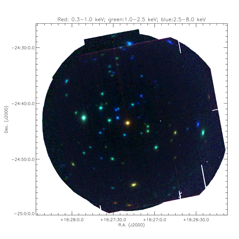
Figure 1: Merged EPIC image of events recorded in the time-filtered data to enhance the signal-to-noise of faint sources. Colors encode the following bands: 0.3-1.0 keV (red), 1.0-2.5 keV (green), 2.5-8.0 keV (blue), respectively. The MOS 1, 2, and PN images are normalized by effective area and exposure time to reduce instrumental artifacts like CCD gaps.

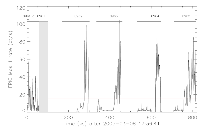
Figure 2: Top panel: light curve of all events recorded with MOS 1. Labels for the individual satellite orbits are given on top of the plot. The gray shaded area represents the time interval when MOS 1 was turned off after the micro-meteorite impact. The horizontal line is the threshold count rate that maximizes the SNR of the full image as described in the text. Bottom panel: signal-to-noise function vs cumulative time.

In order to improve the detection of faint sources, we filtered the data obtained at step 1, excluding those time intervals with a high background count rate. In fact, the background during DROXO was highly variable for a significant fraction of the exposure time (see Fig. 2). We excluded all events registered in intervals when the rate on the whole image, shown in Fig. 2, was higher than a given threshold. The rate threshold was chosen in a way that maximizes the signal-to-noise-ratio (SNR) for faint sources (cf. Sciortino et al., 2001; Damiani et al., 2003) and improves the source detection process toward faint sources as expected. The net cleaned exposure times after this filtering are 198.1 ks (38%) 273.2 ks (53%) and 213.2 ks (41%) for MOS 1, 2 and PN, respectively.

We detected 111 point sources with a significance threshold corresponding to two spurious detections in the whole field-of-view. The threshold for the detection of faint sources was determined from the analysis of a large set of simulations of background-only images and then running the detection code on these images. The simulations provide a value for the significance threshold to retain at most 1-2 spurious sources per field in real data.

Source positions, off-axis distance, exposure times, and X-ray count rates are listed in Table A1 for all detected sources. We also report the 2 MASS designation and other names from the literature for the optical counterparts identified in Sect. 5.1. The last column of Table A1 contains a flag pointing to the source of the previous identifications. We built an atlas of spectra and light curves for each source which is available online; in Appendix LABEL:atlas we show a page of this atlas as an example.

3.2 X-ray spectra

We produced both light curves and spectra of all sources by selecting the photons in circular regions around the source positions. The radii of the regions depend on the source intensity, on possible of nearby sources and the geometry of the CCD. We used regions on the same CCD for source and background; for the background, we avoided to include pixels and columns poorly calibrated in energy. Figure 3 shows two examples of the choice of source and background extraction regions. For PN spectra a further constraint was to have both source and background extraction regions at nearly the same distance from the CCD readout node.

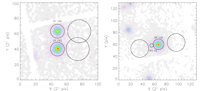
Figure 3: Two examples of choices for the source and background extraction regions. The left panel shows two nearby but distinct sources. The right panel shows an extreme case in which the region for the faint source is shrunk to minimize the influence of the bright source. The background regions are chosen as near as possible to the sources to which they refer and at the same distance of the readout node for PN.

To produce the spectra we filtered the photons with respect to FLAG (chosen to be equal to zero) and PATTERN (less or equal to four) as indicated in the SAS User’s Guide. Given that the choice of GTIs was tailored toward the faintest sources, at this stage we further improved the choice of GTIs for bright sources. The time-filtering we adopted for spectra starts from the Good Time Intervals (GTIs) defined initially to perform source detection and iteratively adds temporal bins from the light-curve that contribute to increase the total SNR of the spectrum. The procedure starts by adding the time bin with the largest individual SNR and is then iterated considering time-bins of decreasing SNR until no gain in total SNR is obtained. As a result, the net exposure time of each spectrum is different.

3.2.1 Background subtraction

We noticed that scaling the background by the geometric areas of the source and background extraction regions leads to incorrect estimates of the background, especially for faint sources and/or during times of high background. The effect is that background-corrected light curves of faint sources are either directly or inversely correlated with the background light curves and often lead to negative net count-rates. We understood this as the effect of a vignetted background component that is not properly taken into account by a purely geometric scaling factor. In order to correctly estimate the background contribution to the photons extracted in the source region we constructed background maps for each instrument (MOS 1, 2 and PN) and for each orbit. These were built by removing large regions around detected sources from the images, and by subsequently smoothing and interpolating the maps over the source extraction areas. Although the resulting scaling factors differ from the purely geometric ones by only a few percent, the difference is relevant in cases when the background dominates the count rate in the source regions and mitigates the above mentioned spurious effects on the light curves.

3.2.2 Model fitting of spectra

We analyzed the spectra of all X-ray sources in the 0.3–10 keV band. For a given EPIC detector (MOS 1, MOS 2 or PN) spectra from all orbits were summed up; analogously, background spectra were obtained; the response matrices and ancillary response files for each spectrum were multiplied and then summed by weighting by the exposure time. The background was scaled according to the procedure described in Sect. 3.2.1.

The spectra were grouped prior to fitting with XSPEC v. 12.3 to obtain at least a minimum SNR in each bin, by considering both source and background photons. In order to obtain the largest number of meaningful grouped spectra we adopted two schemes of grouping procedure based on high and low SNR of the final spectrum. For this purpose we used the same procedure as in the ACIS_EXTRACT package for the analysis of Chandra ACIS data, adapted to our EPIC spectra to take into account the background.

We grouped the spectra using two thresholds for the minimum SNR to be obtained in each bin, i.e. we generated two sets of spectra, one set with a high and one with a low SNR per bin. The minimum SNR in each spectral bin was imposed on the basis of the source count statistics, SNR $\geq 2$ defining our low SNR binning and SNR $\sim 3-5$ defining our high SNR binning. Where possible, we tried to obtain binned spectra with at least eight bins.

The spectra of all detectors were fitted simultaneously. In some cases we had to discard the data of one or two of the three EPIC cameras. These cases occur when a source is on CCDs gaps of one or two cameras, thus leading to a wrong estimate of the point spread function fraction contained in the extraction area.

The spectra were fitted with one-temperature (1-T), two-temperature (2-T) and, in some cases, three temperature (3-T) APEC models (Smith et al., 2001) plus absorption (WABS) (Morrison & McCammon, 1983), the free parameters were the absorption column N_H, the temperatures, and the emission measures. The abundance pattern was fixed to that found in PMS coronae from the Orion Nebula in the COUP survey (Maggio et al., 2007). Only in four cases described below (Elias 29, SR 12, IRS 42, src. 61) a more complex model was required.

For Elias 29 (src. 38) and SR 12A (src 53) the global abundance scaling was left as a free parameter to achieve a better fit. For Elias 29 we confirm an unusually high abundance ($Z\sim Z_{\odot}$) with respect to those found in PMS coronae ($Z\sim 0.2-0.3Z_{\odot}$), as already reported by Favata et al. (2005). The source IRS42 /GY252 (src. 54) is located in the wings of the much brighter X-ray source corresponding to SR 12A (see right panel of Fig. 3). To take account of the contribution by SR 12A we added the best fitting 3-T APEC model multiplied by a constant factor representing the amount of contamination to the model of IRS 42/GY252. This scaling factor was a free fitting parameter. The spectrum of IRS 42/GY 252 itself can be described with a 1-T APEC model. The spectrum and the best-fit model are shown in Fig. 4. As can be seen, IRS 42/GY 252 is highly absorbed and the soft emission is attributed entirely to the contamination by SR 12A. For the source nr. 61 we used a model given by the sum of two differently absorbed APEC models to account for the soft excess visible below 1.0 keV, as discussed in Sect. 6.4 and Fig. 11.

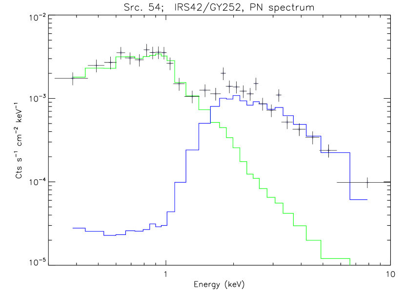
Figure 4: Spectrum and best-fit model of IRS42/GY252. The stepped curves are the contributions of SR 12A (light line) and that of IRS42 (dark line). The spectrum of IRS42/GY252 is modeled by an absorbed single temperature APEC model.

Generally, the best fit was chosen on basis of the probability $P(\chi^{2}>\chi^{2}_{0})$ of obtaining a $\chi^{2}$ higher than the observed one $\chi^{2}_{0}$. Our threshold for acceptable fits was $P(\chi^{2}>\chi^{2}_{0})>0.02$. Whenever this criterion was satisfied by the spectra with high SNR per bin (typically for medium-high statistics spectra) we chose these; otherwise we selected the fits obtained from the spectra with low SNR per bin. We always selected the best-fit model with the smallest number of free parameters. In seven cases, even for some bright sources, no formally acceptable fit was found and we allowed for a lower $P(\chi^{2}>\chi^{2}_{0})$. However, we accepted the best fit results by visually checking that the overall shape of the spectrum is well reproduced by the model.

With this procedure we obtained spectral fits for $91/111$ sources. Table LABEL:t1fit summarizes the results. The columns report the source number, the available EPIC datasets, the data sets we chose for fitting, a flag indicating the binning of the spectra we used (high or low SNR), the type of model, the model best-fit parameters, the unabsorbed flux and luminosity in the 0.3–10 keV band, the $\chi^{2}$ statistics, degrees of freedom and the probability $P(\chi^{2}>\chi_{0}^{2})$. For those weak sources without a spectral analysis, we calculated fluxes and X-ray luminosities in the 0.3–10.0 keV band by using their count rates and PIMMS software assuming a 1-T model with kT and N_H equal to the median of values derived from the best-fit procedure of spectra (see Sect. 4) and a distance of 120 pc.

3.3 Photospheric parameters

In Sects. 5 and 6 we will focus our discussion on the X-ray properties of the sample of PMS stars classified by Bo01. The photospheric stellar parameters ($T_{\mathrm{eff}}$, $L_{\mathrm{bol}}$ and masses) for the Class II and III objects from the list of Bo01 were estimated from the near IR (2MASS) photometry. The procedure we used closely follows that adopted by Bo01 and improved by Natta et al. (2006). We assumed that the J-band emission from these sources is dominated by the stellar photosphere and is only marginally contaminated by the emission from circumstellar material and also that the IR colors of Class II sources can be described as the emission from a passive circumstellar disk as described by Meyer et al. (1997). These assumptions obviously do not apply to Class I sources and for this reason photospheric parameters for these objects were not estimated.

We used the Cardelli et al. (1989) extinction law with R${}_{v}=4.4$, which we think is appropriate for Ophiuchus. A small number of sources ($\sim$15%) have colors slightly bluer than those of reddened main sequence stars, presumably due to photometric uncertainties, which are on the order of 0.1 mag, while the offsets of these objects with respect to the reddened sequence range between 0 and 0.15 mag. Dereddening these sources by extrapolating the colors of Class II and III sources would produce an overestimate of the extinction. For these objects we assigned the colors of the closest photosphere model on the reddened main sequence. Table LABEL:photprop lists the effective temperatures, masses and bolometric luminosities of ISOCAM objects.

The values of the $J$-band extinction we derive are very similar to ones from Natta et al. (2006), with only the significant exception of WL 16, for which our procedure produces a significantly higher extinction.

4 Sensitivity of the survey

The faintest detected source in DROXO has a net count rate of $8.3\cdot 10^{-2}$ ct ks^-1 in MOS equivalent units. In Fig. 5 we plot a sensitivity map in units of count rate per point source of the DROXO field of view. It is built starting from a smoothed background map, after removing the contributions of the sources, and taking into account the vignetted exposure map and the threshold used for detection. The map shows that the sensitivity varies by a factor 2.5 in the area covered by the three EPIC cameras, and it is quite constant across a 60% fraction of the field of view because of the characteristics of the detector. To translate the limit count rate in a limit flux we needed a conversion factor that depends on the spectrum temperature and, critically, on the absorption. From the analysis of the spectra we know that the absorption is also strongly variable from source to source by more than a factor 100, which can be due to local material around the sources or dense cloud material in front of the objects, or both. The plasma temperatures that we find from the spectra vary from $kT\la 1$ keV to a few keV. The combined action of local absorption and plasma temperatures of undetected sources causes the limit flux to vary more than the range observed in the sensitivity map showed in Fig. 5.

For example, we can estimate a conversion factor from count rates to fluxes by using the median of the column absorption ($N_{\mathrm{H}}=2.3\cdot 10^{22}$ cm^-2) and of the plasma temperatures ($kT=3.1$ keV) from the spectral fits, and this gives us $cf=6.1\cdot 10^{-11}$ erg cts^-1 cm^-2. This yields a limiting unabsorbed flux in the 0.3–10 keV band of $\sim 5\cdot 10^{-15}$ erg s^-1 cm^-2 and a luminosity of $\sim 8.7\cdot 10^{27}$ erg s^-1. The $cf$s derived from all sources are in the range $cf=2.3-12.7\cdot 10^{-11}$ erg cm^-2 cts^-1, yielding a limit flux comprised in the range $F_{\mathrm{X}}=5-22\cdot 10-15$ erg cm^-2 s^-1 and luminosities $L_{\mathrm{X}}=7-38\cdot 10^{27}$ erg s^-1, respectively. These values are indicative of the sensitivity we achieved across the field of view, but local strong absorption can significantly lower the actual sensitivity in that position.

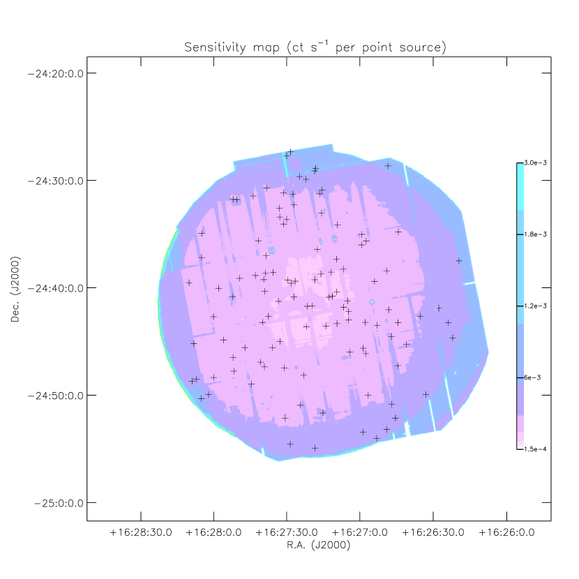
Figure 5: Sensitivity map of the DROXO field in units of ct / s per point source (logarithmic scale). The map refers to the sum of PN and MOS instruments. The intensity scale is indicated in the vertical strip on the right side of the map. Crosses indicate the positions of detected sources.

Figure 6: Left panel: MOS 1 rate from Ozawa et al. (2005) vs. DROXO MOS 1 rate. The lines mark the region for rate variations of factors 2 and 5. Right panel: the same for the ACIS rate from Flaccomio et al. (2003). Upper limits to count rate of sources undetected in the compared samples are indicated by vertical and horizontal arrows. Errors are quoted at 1$\sigma$ level.

4.1 Comparison with other X-ray surveys of $\rho$ Ophiuchi

In Fig. 6 we show the scatter plots of the MOS 1 count rate from Ozawa et al. (2005) and Chandra-ACIS rate (which has an effective area comparable to the EPIC MOS) from Flaccomio et al. (2003) vs. the DROXO MOS equivalent rate. In DROXO we detected 80 of the X-ray sources reported by Ozawa et al. (2005), while 7 of the sources found by Ozawa and collaborators remain undetected in DROXO; analogously we identified 62 sources from Flaccomio et al. (2003), while 30 of those sources have not been detected. We computed an upper limit to the count rates for those sources that are detected by Flaccomio et al. (2003) and Ozawa et al. (2005) but are undetected in DROXO (indicated as arrows in Fig. 6). We also re-analyzed the previous XMM-Newton observation reported by Ozawa et al. (2005) with the same detection procedure as in DROXO, and we calculated the upper limits to count rates for DROXO sources undetected in the Ozawa survey. Analogously we calculated upper limits to count rates for two sources detected in DROXO but undetected by Flaccomio et al. (2003). The count rates of sources detected in DROXO and in the two other surveys globally agree within a factor $\sim$5. Because there is no systematic trend in the scatter we conclude that it is likely to be attributed to variability. Although a detailed study of the time variability is beyond the scope of this paper, we report here that 52% of the sources have variable rates at more than 90% significance level when compared with the Ozawa et al. survey, and 79% are found variable to be compared with the survey of Flaccomio et al.

In the $33$ ks XMM-Newton survey of Ozawa et al. (2005) the faintest detected source has a count rate of 0.5 ct ks^-1. Using the conversion factor derived by us for DROXO the corresponding luminosity is 5.3$\cdot 10^{28}$ erg s^-1, which scales reasonably well with the exposure times of both surveys. Flaccomio et al.’s survey reaches a limiting rate similar to DROXO, likely due to the lower Chandra-ACIS background with respect to that found in our EPIC observation. Most of the ACIS sources undetected in DROXO are near the sensitivity limit of DROXO, and a variability of factor 2 can easily explain their missed detections.

Sources 33 (GY 304) and 43 are brighter in DROXO than in Ozawa et al. survey by more than a factor five. DoAr 25 suffered of strong pile-up in the Ozawa et al. survey. These authors do not report a direct measurement of the count rate for this object, but they derived a luminosity from the spectral analysis. From its X-ray luminosity we inferred a count rate greater than 200 ct/ks. We checked that in DROXO DoAr 25 and the other two brightest sources in the field, SR 12A and IRS 55, are not affected by pile-up. The variability of DoAr 25 with respect to the XMM observation detailed in Ozawa et al. (2005) is at least a factor 4.

Among the most variable sources, WL 2 (labeled in Fig. 6) shows a big flare in the DROXO light curve (Fig. 7). The quiescent rate of WL2 is $\sim 6$ ct ks^-1 and the peak rate is $\sim 300$ ct ks^-1 explaining its large offset position in the scatter plot of the right panel in Fig.6. The quiescent rate is consistent with the one measured by Ozawa et al. (2005). The long duration of this flare on WL 2 ($\sim 35$ ks) underlines the need for long observations of YSOs to properly assess their quiescent emission.

Figure 7: PN Light curve of WL2 (source nr. 15). The bold light curve is the net rate, while the thin line is the total rate (source + background). A large flare lasting $\sim$35 ks is well visible. The source quiescent rate is comparable to the background rate.

5 The nature of the X-ray sources

5.1 Optical and IR counterparts of the DROXO sources

We searched for optical and IR counterparts of DROXO sources in the 2MASS, Spitzer C2D (Evans et al., 2003a) and ISOCAM (Bo01) surveys as well as in the optical and IR surveys of Natta et al. (2006), Wilking et al. (2005), Barsony et al. (2005) and Luhman & Rieke (1999). The match radius takes into account the uncertainties on the X-ray source position in DROXO, which is generally on the order of $\sim 1\arcsec$ , and other catalogs. The mean value for the match radius is $\sim 1.0\arcsec$ with a 0.1-0.9 quantile range of $\sim 0.5--5.8\arcsec$. As anticipated in Sect. 3.1, Table LABEL:tabdet reports the literature names of DROXO counterparts and a flag indicating in which catalogs the source is identified. Sources with counterparts in the ISOCAM survey are indicated with letter “I” in the “Flag” column; sources identified only in Spitzer are indicated with letter “S” ; sources which have only a X-ray identification in the surveys by Flaccomio et al. (2006) and/or Ozawa et al. (2005) are indicated with letter “X”. Among the $111$ X-ray sources $78$ have a counterpart in 2 MASS and $61$ have a counterpart in ISOCAM data. Two objects have no 2 MASS and no ISOCAM counterpart, but have been identified in the literature (IRS50 and WSB46).

An additional $16$ X-ray sources have been newly identified with Spitzer. This leaves $16$ DROXO sources without known optical/IR counterpart. Of these, $6$ were detected in previous X-ray surveys and $10$ are presented here for the first time. We calculated upper limits to the X-ray fluxes and luminosities for the sample of undetected ISOCAM objects falling in the field of view of DROXO using the conversion factor derived in Sect. 4.

5.2 Unidentified X-ray sources

The inspection of light curves and spectra can give some indication on the nature of sources with unknown optical/IR counterpart, designated ‘U’ or ‘X’ in Table LABEL:tabdet. Five unidentified sources (Src. # 5, 7, 16, 26, 58) are too faint for spectral analysis, but the other five unidentified X-ray sources (Src. # 12, 19, 88, 96, 110) have spectral parameters compatible with the expectation for a YSO in $\rho$ Oph, i.e. $kT$ of a few keV and $N_{\rm H}>10^{22}\,{\rm cm^{-2}}$. Furthermore, Src. 110 shows impulsive time variability similar to flares typical for PMS stars. There are also six sources (Src. # 20, 29, 41, 45, 48, 95) without optical/IR counterpart that have been detected in previous X-ray surveys. For Src. # 20, 29 and 41 we had too few counts to obtain meaningful spectral fits, and their light curves show some variability, but no clearly identifiable flare. For Src. # 45, 48 and 95 the spectral analysis gives a high absorption (above 10²² cm^-2). While the temperature of Src. # 95 is not constrained, Src. # 45 and 48 have plasma temperatures of 5.4 and 4.5 keV. For these two sources a power law best fit to their spectra is also acceptable. These three objects could have characteristics consistent with those of highly embedded YSOs, although they are undetected on the millimetric surveys of Motte et al. (1998); Johnstone et al. (2000); Jørgensen et al. (2008). The lack of 2MASS counterparts suggests that these sources could have an extragalactic nature. On the other hand, it is not ruled out tthat they are very low mass PMS stars or even brown dwarfs.

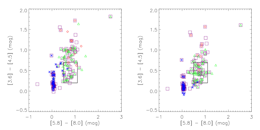
Figure 8: IRAC color-color diagrams of objects in the DROXO field with information on the reddening from J or V band photometry or from $N_{\mathrm{H}}$. The left panel shows colors before correction for the reddening, the right panel shows dereddened IRAC colors. Purple squares mark objects with X-ray emission in DROXO. Asterisks are Class III YSOs, triangles are Class II YSOs and diamonds are Class I YSOs. The rectangle marks the region where Class II YSO colors are expected.

5.3 Mid-IR photometry from Spitzer

The Spitzer photometry for the X-ray sources identified in the C2D survey are listed in Table A4. We derived magnitudes in the 3.6, 4.5, 5.8, 8.0 $\mu$m IRAC bands and constructed the color-color diagram shown in Fig. 8 (color index $[3.6]-[4.5]$ vs color index $[5.8]-[8.0]$). This diagram provides a rough classification of YSOs according to Allen et al. (2004) and Hartmann et al. (2005). Normal, unreddened stars or Class III / Weak T-Tauri stars with very low reddening should occupy a region centered around (0,0). Reddening due to matter along the line of sight tends to disperse vertically data points along the [3.6]$-$[4.5] IRAC color index, while the [5.8]$-$[8.0] color index is not affected by this source of reddening (see Flaherty et al., 2007). Infrared emission from a circumstellar disk in Class I and II sources moves the objects both vertically and horizontally toward redder values of both indexes. We expect to find Class II YSOs in the region marked with the black box or above it and very embedded protostars (Class 0/I) are expected to lie at $[3.6]-[4.5]\ga$ 1.1 and at $[5.8]-[8.0]>1$ (Allen et al., 2004).

We plotted only the objects for which we have information on the reddening from J and V band photometry or from $N_{\mathrm{H}}$. In the left panel of Fig. 8 the symbols represents the IRAC colors before correction for reddening. Objects detected in DROXO are marked with squares, diamonds are Class I YSOs as classified by Bo01, triangles are Class II YSOs, asterisks are Class III YSOs. The points with ISOCAM classification follow the distribution outlined above, with Class III YSOs around or dispersed vertically above the (0,0) point, and Class II YSOs located in the rectangle or dispersed vertically above this region.

In order to investigate the nature of these latter “dispersed” objects we dereddened the colors of those objects for which we had information on the extinction. If available we used the reddening $A_{\mathrm{J}}$ or $A_{\mathrm{V}}$ from the literature, otherwise the column absorption $N_{\mathrm{H}}$ from the X-ray spectra with the conversion factor of $A_{V}=1.51\cdot 10^{-22}\cdot\mathrm{N}_{h}$ (Mathis, 1990). To convert these extinctions to the Spitzer bands we followed the calibrations by Flaherty et al. (2007) and Carpenter (2001). The relation between reddening in 2MASS K_s and IRAC bands provided by Flaherty et al. (2007) for $\rho$ Ophiuchi indicates that no reddening is present in the $[5.8]-[8.0]$ color index. Therefore, dereddening shifts the objects vertically downwards in Fig. 8. The right hand panel of Fig.8 shows the dereddened IRAC colors. Evidently, most objects with $[3.6]-[4.5]>0.7$ in the left hand side of Fig. 8, fall in the “canonical” IRAC Class II area after dereddening. Therefore, the majority of objects with apparently protostellar IRAC colors are probably strongly reddened Class II sources. We note also that the ISOCAM sub-sample without X-ray counterparts has the same color distribution as the ISOCAM/DROXO sample. This indicates that no bias is present against X-ray properties.

Prisinzano et al. (2008) found that Class I protostars in the Orion Nebula can be separated into two distinct subclasses: the first, Ia, with a rising SED from $K$ to 8$\mu$m and lower X-ray emission level than the second one, Ib, characterized by rising SED up to 4.5$\mu$m. This latter group shows IRAC colors more similar to those of Class II objects. The first subclass, Class Ia, is instead populated by more embedded protostars with lower and, perhaps, more absorbed X-ray emission. They find 23 Class 0-Ia YSOs, 22 Class Ib YSOs and 148 Class II YSOs. In COUP the fraction of Class Ia on Class II YSOs is $\sim 16\%$, the fraction of Class I versus Class II YSOs in Orion is $\sim 30\%$. In DROXO the fraction of Class I objects with [3.6]-[4.5] $>1$ (after dereddening) is $\sim 7\%$ with respect to Class II objects. This sample should be composed by very embedded objects similar to Class Ia defined by Prisinzano et al. (2008). The number of very embedded protostars in Core F of $\rho$ Ophiuchi is thus very low with respect to Class II objects. The same evidence has been obtained by Jørgensen et al. (2008). In that paper the fraction of Class I to Class II is reported to be lower in $\rho$ Ophiuchi than that present in other star-forming regions like Perseus (10% in $\rho$ Ophiuchi vs 90 % in Perseus, respectively), hinting for a different age or formation time-scales for these two star-forming regions.

Three objects (GY92, GY289, GY203) which have been classified as Class III by Bo01 are found with Spitzer colors similar to Class II YSOs. Furthermore, we find three objects classified as Class II YSOs (GY 146, GY 240, GY 450) that are bluer than 0.4 mag in ([5.8] - [8.0]) IRAC color. These objects may have transition disks (see Kim et al., 2009, and references therein). The star with the reddest IRAC colors located in the top right corner of Fig. 8 is WL22/GY174. It is classified as a Class II object and probably it suffers of strong foreground extinction as pointed out by Wilking et al. (2001). This is supported also from our spectral fit to its X-ray spectrum: we find a N_H absorption value of $1.3\cdot 10^{23}$ cm^-2, a factor of 5 higher than the average of the DROXO sample.

6 Results

6.1 Coronal temperatures and absorption

Table LABEL:t1fit lists the temperatures obtained through a thermal model fit to the X-ray spectra as described in Sect. 3.2.2. Most of the spectra are reasonably well described by a model with a single thermal component; usually we find temperatures higher than 1.5 keV and absorption column N_H higher than $10^{22}$ cm^-2. In a few cases two or three thermal components are needed to fit the spectra, depending on the characteristics of the spectrum and its count statistics. For these cases we calculated the average of the two or three plasma temperatures weighted by their emission measures to obtain a representative mean temperature for these spectra. The median of the representative plasma temperatures is $\sim$3.1 keV with a 1$\sigma$ range between 1.6 and 8 keV (the 10%–90% quantile range is 0.8–13 keV). The 10%–90% quantile range of the N_H column is $2.8\cdot 10^{21}-7.2\cdot 10^{22}$ cm^-2 and the median is $2.3\cdot 10^{22}$ cm^-2.

6.2 X-ray luminosities and stellar parameters

We examine the relation between X-ray luminosity and X-ray to bolometric luminosity ratio and mass and effective temperature for all X-ray sources for which stellar parameters could be determined in Sect. 3.3 (Fig. 9).

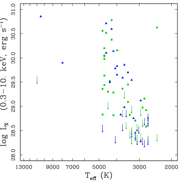
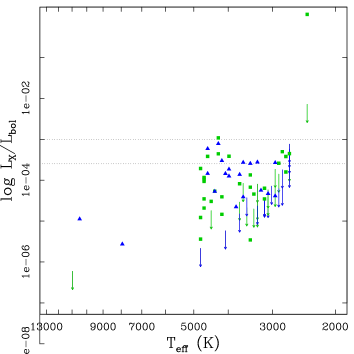
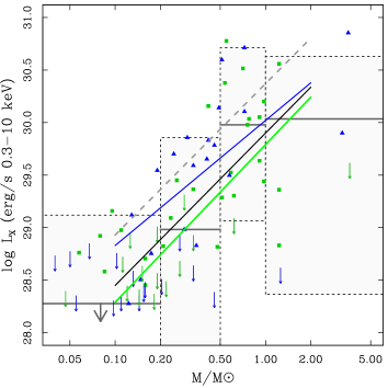
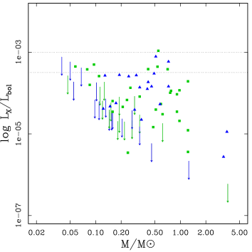
Figure 9: Top left panel: X-ray luminosities (0.3-10. keV) versus effective temperatures of YSOs identified with ISOCAM objects (Bo01). Symbols are: squares Class II YSOs, triangles Class III YSOs. Upper limits to luminosities were calculated for ISOCAM objects not detected in DROXO (vertical arrows). Top right panel: $L_{\mathrm{X}}/L_{bol}$ ratios vs $T_{\mathrm{eff}}$. The upper limit with highest $T_{\mathrm{eff}}$ and mass is relative to WL 16 and calculated taking into account an $A_{\mathrm{V}}\sim 30$ mag and a $kT=1$ keV (see text). The detection point at the lowest $T_{\mathrm{eff}}$ is from WL 2 that exhibited the large flare shown in Fig. 7. Bottom left and right panels: X-ray luminosities and $L_{\mathrm{X}}/L_{bol}$ vs. mass (in units of $M_{\odot}$). The boxes in the left panel are the 10%$-$90% quantile ranges of luminosities derived from the Kaplan-Meier estimator of XLFs in four mass ranges ($\leq 0.2$, 0.2–0.5, 0.5–1.0, $\geq 1.0M_{\odot}$). Horizontal segments mark the median of $L_{\mathrm{X}}$ in each mass interval, in the lowest mass bin the median is an upper limit. The solid black line is the relation between mass and luminosity fitted between 0.1 and 2 M_⊙, blue and green lines are the best fits for Class III and Class II YSOs respectively. The dashed gray line is the analogous obtained by Preibisch et al. (2005) to Orion young stars. Horizontal lines in the bottom right panel are the values of saturation of $\log L_{\mathrm{X}}/L_{\mathrm{bol}}$ equal to -3 and -3.5.

The X-ray luminosities for the sample with known stellar parameters increase from $\sim 2\cdot 10^{28}$ ergs s^-1 up to $\sim 7\cdot 10^{30}$ ergs s^-1 in the 3000–5000 K range (Fig. 9, top left panel) or $\sim 0.1-0.7$ M_⊙ (left bottom panel). Most of the YSOs have effective temperatures around 3000–5000 K (K type stars), with the exception of the three hot stars WL 5, WL 16 and WL 19. The fraction of X-ray detections among ISOCAM YSOs increases from $\sim 0.1M_{\odot}$ to $\sim 1M_{\odot}$. The boxes in the bottom left panel of Fig. 9 are the 10–90% quantiles obtained with ASURV software (Schmitt, 1985; Lavalley et al., 1992) for $\log L_{\mathrm{X}}$ values in four ranges of mass ($<0.2$, $0.2-0.5$, $0.5-1.0,>1.0$ $M_{\odot}$). For these mass ranges the median values of $\log L_{\mathrm{X}}$ are $\leq$28.3, 29.0, 30.0 and 30.0, respectively. The COUP sample contains very few upper limits in each mass range whereas in DROXO the fraction of upper limits is $\sim 30$ % reducing the $L_{\rm x}$ medians in each mass range. As discussed below in Sect. 6.3, we suggest that a fraction of Class III YSOS are likely spurious cloud members. We fitted the relation between X-ray luminosity and mass excluding these suspect members in the Class III sample obtaining $\log L_{\mathrm{X}}\sim 29.9\pm 0.2+\log M^{(1.45\pm 0.25)}$ with the same procedure used by Preibisch et al. (2005) for COUP sample. We also fitted X-ray luminosity and mass relation for Class II and Class III samples separately, finding similar slopes but different normalizations. The relations are
$\log L_{\mathrm{X}}\sim 29.8\pm 0.2+\log M^{(1.5\pm 0.3)}$ and
$\log L_{\mathrm{X}}\sim 30.0\pm 0.3+\log M^{(1.2\pm 0.5)}$
for Class II and Class III YSOs respectively. The slopes of these relations are very similar to those found for ONC in COUP program (1.44, Preibisch et al., 2005). The lower normalizations that we find in the $\rho$ Ophiuchi sample with respect to ONC (up to 0.6 dex for DROXO Class II objects with respect to COUP) can be due to systematic effects like distance estimate (for Orion it was used a value of 450 pc, more recent estimates place ONC to $\sim$400 pc, see Sect. 8.1.1 in Mayne & Naylor, 2008, and references therein) and correction for absorption, but an intrinsic difference could be present. Thus PMS stars in $\rho$ Ophiuchi are on average less luminous than PMS stars in Orion. Because there are upper limits in DROXO, this difference should be more marked. Also in the Taurus Molecular Cloud (TMC) Telleschi et al. (2007) find a power law index of $\sim 1.5$ between $\log L_{\mathrm{X}}$ and mass.

The $\log L_{\mathrm{X}}/L_{\mathrm{bol}}$ ratio increases with decreasing stellar masses (Fig. 9, bottom and top right panels) saturating at $\sim-3.5$ for stars cooler than 5000 K and with masses of $\sim 0.7$ M_⊙, slightly below the “canonical” value of ${-3}$ observed in MS young stars, but very similar to the value reported by Preibisch et al. (2005) for Orion YSOs (${-3.6}$).

From the relation between mass and X-ray luminosity and the hypothesis that the ratio $\log L_{\mathrm{X}}/L_{\mathrm{bol}}$ for PMS stars is saturated at a level of $-3.5$, Telleschi et al. (2007) derived an empirical mass – bolometric luminosity relation for PMS stars $\log L_{\mathrm{bol}}\sim\log(M/M_{\odot})^{1.49}$ which is shallower than the relation that yields for MS stars. By considering that the saturation limit of $\log L_{\mathrm{X}}/L_{\mathrm{bol}}$ for our sample of YSOs of $\rho$ Ophiuchi is similar to that of TMC and ONC ($\sim-3.5$, see fig. 9) and that the slope of the relation between mass and $L_{\mathrm{X}}$ is quite similar for $\rho$ Ophiuchi, ONC and TMC, it is suggested that the relation between mass and $L_{\mathrm{bol}}$ found from Telleschi et al. (2007) for coeval PMS stars should apply also for our sample.

Among the three hottest stars, characterized by effective temperatures around 10000 K, we detected the Class III YSOs WL 19 and WL 5, while WL 16 (Class II) remains undetected. X-ray spectra of WL 19 and WL 5 show quite hot plasma temperatures (kT= 3.7 keV and 4.5 keV, respectively) and high absorption (N${}_{H}=10^{23}$ and 6.5$\cdot 10^{22}$ cm^-2, respectively). The undetected Class II YSO WL 16 is a peculiar object: it consists of a massive star (L$=250$L_⊙, $M\sim 4$M_⊙) that illuminates a circumstellar disk visible only at mid-IR wavelengths (Ressler & Barsony, 2003). It suffers of strong absorption ($A_{V}\geq 30$) likely due to a foreground screen of cloud material. Taking into account this high absorption, the upper limit to luminosity is inversely correlated with the plasma temperature: for $kT=4$ keV we obtain $\log L_{\mathrm{X}}\la 28.8$, for $kT=1$ keV $\log L_{\mathrm{X}}\la 29.6$, for $kT=0.5$ keV $\log L_{\mathrm{X}}\la 30.7$. According to their position in the HR diagram these three objects are intermediate-mass pre-MS stars and their X-ray luminosities and $L_{\mathrm{X}}/L_{\mathrm{bol}}$ ratios are in the range typically observed for Herbig Ae/Be stars (Stelzer et al., 2009).

The coolest object is the binary system WL2/GY128 (Barsony et al., 2005). A discrepancy between its spectral type and the effective temperature is present in the literature. While its spectral type is comprised between K and M as reported by Luhman & Rieke (1999), its temperature, estimated by Natta et al. (2006), is very low ($\sim$2300 K). As discussed in Sect. 4.1, WL 2 has undergone a huge flare during DROXO. Its quiescent X-ray luminosity is $\sim 10^{29}$ erg s^-1 which is typical for young K–M type stars but unexpectedly high for a low mass brown dwarf. Likely the photospheric temperature of this object is more similar to that of late K or M-type stars.

Only two bona fide brown dwarfs are in the field of view. We detected GY 310 (log $L_{\mathrm{X}}=28.92$ erg s^-1), but not GY 141, which was detected by Ozawa et al. (2005) during a flare with a flux 90 times higher than in a previous Chandra observation.

6.3 X-ray emission of different YSO classes.

We examined the X-ray detection rates for YSOs in different evolutionary states referring to the YSO classification of Bo01. Their catalog comprises 16 Class I, 123 Class II, and 38 bona-fide Class III. The latter are classified as Class III YSOs on the basis of absence of IR excess and detection in X-ray images (ROSAT) and/or radio band (VLA). Given the low ROSAT sensitivity at $L_{\mathrm{X}}\sim 3\cdot 10^{29}$ erg s^-1 the sample of Class III YSOs is presumably incomplete. Bontemps et al. (2001) report also a list of 39 candidate Class III stars which are objects with stellar-like colors. They are found in the dense part of the cloud and have no X-ray detection at the ROSAT sensitivity limit. Bontemps et al. (2001) conclude that these objects are in excess with respect to the number of expected field stars because of the high extinction in the region where they lie, and for this reason these objects were assumed Class III star candidates. For the detection rates we considered only the fraction of $\rho$ Oph members that are within the DROXO field-of-view (col. 2 of Table 1). The number of X-ray-detected stars from each YSO group is given in Col. 3, and the detection fraction is summarized in Col. 4. The last two columns of Table 1 provide the medians of the plasma temperatures and of X-ray luminosities for each sub-sample. These last values were obtained with ASURV and take into account the upper limits for non-detected objects. Before proceeding to a discussion of the numbers given in Table 1 an assessment of biases and completeness is in order. The ISOCAM sample is not well suited to select Class III sources. The evidently low X-ray detection rate of candidate Class III stars from Bo01 suggests that most of them are spurious members. We detected six Class III candidates with $\log L_{\mathrm{X}}>28.3$, and found that they have Spitzer photometry consistent with Class III objects . There remain 15 out of 21 Class III candidates undetected at $\log L_{\mathrm{X}}<28.3$. Their masses are comprised between 0.1 and 0.5 $M_{\odot}$, and their dereddened IRAC colors [3.6] – [4.5] are comprised between 0.0 and 0.2 mag, whereas the six X-ray-detected Class III candidates have [3.6] – [4.5] colors up to 0.4 mag. In the following discussion we will also consider a sub-sample of Class III objects without the 15 X-ray-undetected Class III candidates.

Previous studies of star-forming regions have shown that for each given mass range, Class I and II YSOs show lower X-ray luminosities than Class III YSOs (Neuhäuser et al., 1995; Flaccomio et al., 2003; Preibisch et al., 2005; Telleschi et al., 2007; Prisinzano et al., 2008). Figure 10 (top left panel) shows the Kaplan-Meier estimators of X-ray luminosity function (XLF) of Class I, II, and III objects following the Bo01 classification. Upper limits are mostly concentrated below the lowest detection values for Class II and III YSOs. We plot also the XLF of Class III YSOs (dots and dashed line) after excluding 15 upper limits of Class III YSO candidates from Bo01. In this way we try to correct the bias introduced by spurious members that very likely contaminate the Class III YSO sample as discussed above. This corrected Class III XLF is similar to the XLF of Class I YSOs. The corrected Class III XLF shows higher luminosity levels with respect to Class II XLF. Two sample tests yield a probability of $\geq 99\%$ for the two distributions of being different, thus suggesting that in $\rho$ Ophiuchi Class III YSOs are more luminous than Class II YSOs. We observe also that Class I YSOs have similar X-ray luminosity levels compared with Class III objects. The high X-ray detection rate and high X-ray luminosities among Class I objects are surprising. For comparison, in ONC Prisinzano et al. (2008) have found that the X-ray luminosities of Class I are lower than those of more evolved Class II YSOs. Our X-ray bright Class I YSOs could be explained as an effect of different mass distributions in different samples but, given that we cannot estimate masses of Class I objects with our method, we cannot test this hypothesis.

Table 1: X-ray detection rates and median of logarithm of X-ray luminosities and plasma temperatures for the different YSO groups following the classification given by Bontemps et al. (2001).

YSO Class	$N_{\rm DROXO,FOV}$	$N_{\rm det}$	detection	$\log\rm L_{\rm x,med}$	median kT
			fraction	[erg/s]	keV
I	11	9	82 %	29.6	4.4
II	48	31	77 %	28.8	3.1
bona-fide III	16	15	94 %	29.7	2.4
candidate III	21	6	29 %	$\leq 28.3$	–
Total	96	61	64%

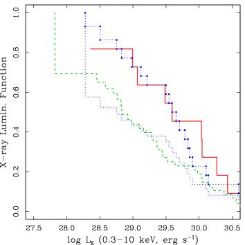
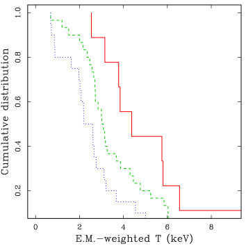
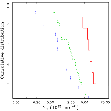
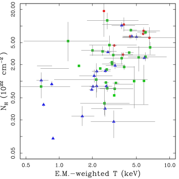
Figure 10: Top left panel: Kaplan-Meier estimators of cumulative distributions of $L_{\mathrm{X}}$ for Class I YSOs (solid line), Class II YSOs (dashed line), Class III YSOs (dotted line) and corrected XLF (dotted line + points) of Class III YSOs from Bo01. Top right panel: cumulative distribution of mean plasma temperatures obtained from fit to spectra for Class I (solid line), Class II (dashed line), Class III (dotted line) objects. Bottom left and right panels: cumulative distributions of $N_{\mathrm{H}}$ column absorption among the different classes (left) and scatter plot of mean plasma temperatures vs. $N_{\mathrm{H}}$ (right). Circles are Class I YSOs, squares are Class II YSOs, and triangles are Class III YSOs.

The distribution of mean plasma temperatures in Fig. 10 (top right panel) shows that on average the emitting plasma in Class I YSOs is hotter than in Class II and Class III YSOs. The median plasma temperatures for Class I, II and III are reported in Table 1. Two-sample tests give a probability of $99\%$ to reject the null hypothesis that the distributions of temperature for Class III and Class I YSOs are drawn from the same distribution, the probability is $\sim$98% when comparing Class II and Class I temperatures, and $\sim 90\%$ when comparing Class II and Class III YSOs temperature distributions. As expected, the distributions of $N_{\mathrm{H}}$ show that the absorption is higher on average in Class I YSOs than in Class II and III (see Fig. 10 bottom left and right panels), indicating circumstellar matter in Class I objects.

6.4 Source with a soft X-ray excess

We discuss the case of the source nr. 61, which shows an excess of soft photons in the 0.3–1.0 keV band significantly different from a typical coronal singly-absorbed multi-temperature plasma. This object has no counterpart in the ISOCAM survey, although in the literature is identified with GY 266 and is classified as a variable star by Alves de Oliveira & Casali (2008). Furthermore, it has an IR counterpart in 2MASS and Spitzer catalogs. From IRAC and MIPS photometry this object is cataloged as a normal star (Evans et al., 2003b). The DROXO spectrum of this object is shown in Fig. 11. We modeled the spectrum with two thermal components, which were differently absorbed. The soft component has kT = $0.47_{0.23}^{0.67}$ keV ($\sim 5.5$ MK) and is absorbed by a N_H column of $\sim 3_{0.}^{34}\cdot 10^{20}$ cm^-2. This is one of the softest thermal components we have determined in the whole sample of DROXO spectra. The hot component has kT = 1.8${}_{1.4}^{2.4}$ keV absorbed by N${}_{\mathrm{H}}\sim 2.5_{2.1}^{3.2}\cdot 10^{22}$ cm^-2. The emission measure ratio of soft to hot component is $\sim 1\%$. The hot component has the typical temperature and column density of a YSO in $\rho$ Oph, whereas the weakly absorbed component is unusually soft.

Güdel et al. (2007) have reported similar examples of X-ray spectra with soft excess from the XEST survey. They modeled them with a 2-T plasma with individual absorptions and hypothesized that the soft component be associated to the emission from shocks in jets. Bonito et al. (2007) have studied the soft X-ray emission that could arise from bipolar jets in YSOs through extensive MHD simulations. They find that a jet less dense than the ambient medium in which it propagates can emit soft X-rays with plasma temperatures of 2-3 MK, very similar to that of the soft component we found. Moreover, Bally et al. (2003) and Favata et al. (2006) observed that the X-ray emission of HH 154 jet is located at the base of the shock and that morphological changes are detected on a time scale of four years. The X-ray luminosity of that jet is $4\cdot 10^{29}$ erg s^-1. In our case the unabsorbed luminosity of the soft component in the spectrum of GY 266 is much lower than that of HH 154 (3.4$\cdot 10^{27}$ erg s^-1). Given the angular resolution of EPIC we cannot spatially resolve the soft component from the hot component. Thanks to angular resolution of Chandra (Güdel et al., 2008) resolved separated soft emission from the coronal emission in the star DG Tau belonging to the Taurus Molecular Cloud. The coincidence of the elongated soft X-ray emission with the direction of the optical jet represents a clear case for the jet scenario in DG Tau. In our case the lack of IR excess is difficult to reconcile with the circumstellar disk, which is expected along with the jet. Explaining the origin of the X-ray soft component of GY 266 requires further investigation of this star.

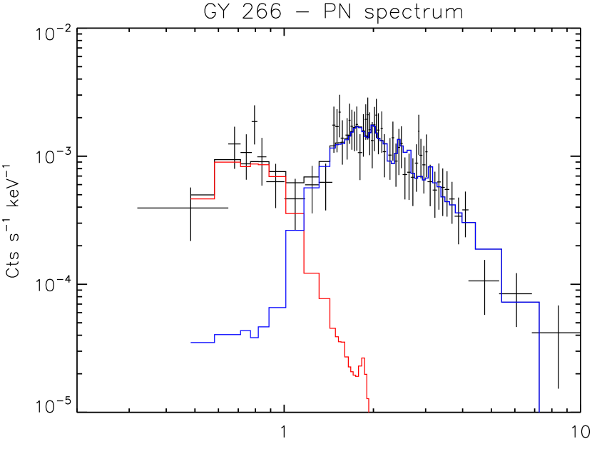
Figure 11: X-ray spectrum of source # 61 (GY 266) with a soft component in the 0.3–1 keV energy range, less absorbed than the hot component.

7 Discussion and conclusions

We described the Deep Rho Ophiuchi XMM-Newton Observation (DROXO), aimed at exploring at high sensitivity the X-ray emission of YSOs in the $\rho$ Ophiuchi core F region. We detected 111 X-rays sources, and for 91 of them we obtained a model fit to their X-ray spectra. By using optical and IR data we estimated the photospheric parameters of most of the sample of X-ray detected YSOs.

We find 10 unidentified sources and a further 6 sources already detected in previous X-ray surveys, but without optical/IR counterpart. Three of them (src. num. 45, 48 and 95) show light curves with some impulsive variability. The spectra of src. num. 45 and 48 have a good fit with an absorbed power law, while src. num. 95 has a spectrum compatible with a thermal model. The lack of 2MASS counterparts could be a hint that they are of extragalactic nature, but, given the sensitivity of 2MASS catalog, it is not possible to rule out they are very low mass PMS stars or even brown dwarfs, especially src. num. 95.

The sensitivity of the survey is $f_{\mathrm{X}}\sim 5\cdot 10^{-15}$ erg s^-1 cm^-2 in flux and log $L_{\mathrm{X}}$ (erg s${}^{-1})\sim 27.9$ in luminosity, but it strongly depends on the local absorption, which is largely variable in the field-of-view. The sample of 96 classified YSOs given by Bo01 in the DROXO field of view has allowed us to explore the X-ray emission from Class I, II, and III YSOs of $\rho$ Ophiuchi. The X-ray properties of $\rho$ Ophiuchi PMS stars obtained from DROXO were compared with those of the Orion Nebula Cloud PMS stars studied in the COUP survey. When fitting the relation between mass and X-ray luminosity with a power law, the index that we find for DROXO sample is quite similar to that found for ONC and TMC (Preibisch et al., 2005; Telleschi et al., 2007). With respect to COUP we find a lower normalization, suggesting that on average the PMS stars in the range of masses between 0.1–2 $M_{\odot}$ in our sample are less luminous than their analogs in COUP. Young stellar objects in $\rho$ Ophiuchi exhibit a saturation of the ratio L${}_{\mathrm{X}}/$L_bol near the “canonical” value of $\sim 10^{-3}$ for masses between 0.5 and 1 M_⊙, while stars with masses below 0.5 M$\odot$ show a lower limit of saturation L${}_{\mathrm{X}}/$L${}_{\mathrm{bol}}\sim 10^{-3.5}$. This is consistent with what was found by Preibisch et al. (2005) for the COUP sample.

We detected a large fraction of YSOs in the field of view, 94% of which are bona fide Class III stars, 77% of Class II and 82% of Class I YSOs, respectively. We confirm the high detection rate among Class I YSOs found by Imanishi et al. (2001). The detection rate in our Class I sample is higher than the analog rate found in the COUP survey by Prisinzano et al. (2008) (82% vs. 62%) despite the higher sensitivity of COUP with respect to DROXO. Prisinzano et al. (2008) make a distinction between Class Ia (characterized by a rising SED from $K$ to 8$\mu$m) and Class Ib (rising SED up to 4.5$\mu$m). The detection rates in these two subclasses are 44% and 82% respectively. X-ray luminosities of Class Ib objects are higher than those of Class Ia objects. The rate of X-ray detection of Class Ib objects in Orion is identical to that of our sample of Class I objects in $\rho$ Ophiuchi. With support of Spitzer photometry we suggest that only a small fraction of our Class I stars are deeply embedded objects. From X-ray data the high detection rate suggests that our Class I sample could be mainly formed by Class Ib YSOs as defined by Prisinzano et al. (2008). These objects in Orion have X-ray luminosities more similar to Class II objects. In $\rho$ Oph we find that our nine detected Class I stars are on average more luminous than Class II stars.

Bontemps et al. (2001) list 39 stars defined as Class III candidates, 21 of which are surveyed in DROXO. Six out of 21 are detected in DROXO, providing support for their PMS nature. The other 15 are undetected below $\log L_{\mathrm{X}}=28.3$. Likely they are not PMS stars and thus not members of the $\rho$ Oph cloud. By means of XLFs we evaluated the level of emission of Class I, II, and III YSOs. After excluding the suspect Class III YSOs, we find that Class I YSOs emit at the same level of Class III YSOs (median $\log L_{\mathrm{X}}\sim{29.6}$ and 29.7, respectively) and both samples are more luminous than Class II YSOs (median $\log L_{\mathrm{X}}$ $\leq{28.8}$). In COUP Class III objects are more luminous than Class I and II for masses between 0.5 and 1.2 M$\odot$, while for masses in 0.1-0.5 M$\odot$ Class Ib sources are slightly more luminous than Class II and III (see Fig. 8 in Prisinzano et al., 2008).

The analysis of X-ray spectra leads us to conclude that the mean plasma temperatures of Class I protostars are higher than in Class II and Class III YSOs. We find a clear trend of decreasing plasma temperatures passing from Class I to Class III objects, differently from what is observed in ONC where Prisinzano et al. (2008) do not find a significant evolution of temperatures from Class I to Class III objects. Four Class III stars and one Class II star (GY 112, SR 12A, GY 296, GY 380 and GY 3) have spectra noticeably softer than the rest of YSOs with mean temperatures around 0.7-0.8 keV.

The absorption derived from X-ray spectra is higher in Class I than in Class II and III. Given the high absorption among Class I YSOs, it is impossible to determine if a soft thermal component in their spectra is completely absorbed or is not present at all. This soft component would reduce the intrinsic $kT$ for Class I objects, making them more similar to the ones in the ONC. However, higher absorption should lead to an underestimate of the luminosities of heavily absorbed spectra like those of Class I objects, while we observe a luminosity for them higher than that of in Class II and Class III YSOs. Furthermore, Prisinzano et al. (2008) have found in extensive simulations that varying $N_{\mathrm{H}}$ does not significantly influence the XLF.

The star GY 266 shows a peculiar X-ray spectrum composed by two thermal components that are differently absorbed. The hot and heavily absorbed component is similar to that found in other PMS stars, while the soft one, less absorbed, could arise from unresolved jet shocks.

Appendix A Online tables

Table 2: List of sources detected in the DROXO EPIC images. The columns refer to X-ray positions, position accuracy, summed exposure times from the three EPIC cameras, count rates scaled to MOS detector units (see Sect. 3.1) with 1$\sigma$ errors, 2MASS identifier, ISOCAM identifier, SED classification given by Bontemps et al. (2001), literature names, flag column for identifications (see footnote). Coordinate errors take into account position uncertainties calculated by the detection code and the best-match radius from the optical/IR objects. Class III candidates from Bo01 are indicated by ”III?”.

DROXO source number	R.A.	DEC	Pos. Error	Off-axis	Exp. Time	Rate	2MASS id.	ISOCAM id.a	CLASS	Name	Flagb
	J2000	J2000	$\arcsec$	$\arcmin$	ks	ct/ks
1	16:26:19.4	$-24$:37:29.0	3.5	13.3	137.6	2.6 $\pm$ 0.2	16261949$-24$37275	–			S
2	16:26:21.9	$-24$:44:39.1	3.1	13.2	155.8	1.0 $\pm$ 0.1	16262189$-24$44397	32	II	GY3	I
3	16:26:23.7	$-24$:43:14.3	1.3	12.4	207.7	54.7 $\pm$ 0.6	16262367$-24$43138	38	II	DoAr25/GY17	I
4	16:26:27.6	$-24$:41:53.9	1.2	11.3	249.9	20.6 $\pm$ 0.3	16262753$-24$41535	43	II	GY33	I
5	16:26:32.9	$-24$:49:55.9	7.9	14.0	199.4	0.55 $\pm$ 0.1		–			U
6	16:26:35.3	$-24$:42:38.5	3.8	9.8	297.6	3.0 $\pm$ 0.1		–			S
7	16:26:40.9	$-24$:45:15.5	9.3	9.6	299.3	0.77 $\pm$ 0.1		–			U
8	16:26:44.3	$-24$:34:48.3	3.0	9.1	305.3	0.56 $\pm$ 0.07	16264419$-24$34483	65	I	WL12/GY111	I
9	16:26:44.3	$-24$:43:14.9	1.2	8.0	359.5	11.8 $\pm$ 0.2	16264429$-24$43141	66	III	GY112	I
10	16:26:44.4	$-24$:47:14.7	2.1	10.2	271.0	1.8 $\pm$ 0.1	16264441$-24$47138	–			S
11	16:26:45.3	$-24$:52:07.8	6.5	14.0	193.4	2.8 $\pm$ 0.2		–			S
12	16:26:47.0	$-24$:50:51.5	9.7	12.7	233.5	0.85 $\pm$ 0.1		–			U
13	16:26:47.0	$-24$:44:31.6	3.2	8.1	257.3	1.7 $\pm$ 0.1	16264705$-24$44298	69	III	GY122	I
14	16:26:48.2	$-24$:42:02.8	3.1	6.8	393.0	1.3 $\pm$ 0.09	16264810$-24$42033	–			S
15	16:26:48.5	$-24$:28:39.6	1.9	13.2	120.4	24.4 $\pm$ 0.6	16264848$-24$28389	70	II	WL2/GY128	I
16	16:26:48.9	$-24$:53:11.7	9.6	14.5	222.6	2.3 $\pm$ 0.2		–			U
17	16:26:49.0	$-24$:38:25.0	2.6	6.5	396.8	0.67 $\pm$ 0.06	16264897$-24$38252	72	II	WL18/GY129	I
18	16:26:53.0	$-24$:43:29.9	8.3	6.4	301.4	0.3 $\pm$ 0.06		–			S
19	16:26:53.0	$-24$:54:01.4	2.3	14.9	218.9	0.48 $\pm$ 0.06		–			U
20	16:26:54.0	$-24$:39:24.1	4.4	5.2	443.3	0.32 $\pm$ 0.05		–			X
21	16:26:56.5	$-24$:50:00.0	5.0	10.9	316.9	0.38 $\pm$ 0.06		–			S
22	16:26:57.4	$-24$:35:39.7	2.5	6.3	399.7	0.72 $\pm$ 0.06	16265733$-24$35388	84	II	WL21/GY164	I
23	16:26:57.6	$-24$:46:07.6	1.7	7.4	324.6	0.28 $\pm$ 0.04	16265752$-24$46060	–			S
24	16:26:57.7	$-24$:43:13.4	7.9	5.3	483.2	0.7 $\pm$ 0.07		–			S
25	16:26:58.6	$-24$:45:37.7	1.0	6.9	443.7	24.2 $\pm$ 0.3	16265850$-24$45368	88	II	SR24N$-$SR24S	I
26	16:26:58.7	$-24$:53:26.4	7.1	13.9	171.7	0.77 $\pm$ 0.1		–			U
27	16:26:59.2	$-24$:35:01.7	1.9	6.5	355.3	2.0 $\pm$ 0.1	16265916$-24$34588	90	II	WL22/GY174	I
28	16:26:59.3	$-24$:36:00.6	4.2	5.7	324.2	0.69 $\pm$ 0.09	16265904$-24$35568	89	II	WL14/GY172	I
29	16:27:04.2	$-24$:45:59.7	4.9	6.5	293.4	0.36 $\pm$ 0.05		–			X
30	16:27:04.6	$-24$:43:00.6	1.1	4.0	539.4	12.6 $\pm$ 0.2	16270451$-24$42596	96	III	GY193	I
31	16:27:04.6	$-24$:42:13.6	1.2	3.5	547.0	8.38 $\pm$ 0.1	16270456$-24$42140	97	III	GY194	I
32	16:27:05.0	$-24$:41:14.0	4.7	2.9	376.3	0.22 $\pm$ 0.04		–			S
33	16:27:06.6	$-24$:41:49.8	1.8	2.9	304.4	0.69 $\pm$ 0.06	16270659$-24$41488	102	II	GY204	I
34	16:27:06.8	$-24$:38:16.4	2.3	2.9	531.6	0.75 $\pm$ 0.05	16270677$-24$38149	103	II	WL17/GY205	I
35	16:27:09.2	$-24$:34:09.0	1.6	6.2	338.4	3.8 $\pm$ 0.1	16270910$-24$34081	105	II	WL10/GY211	I
36	16:27:09.4	$-24$:43:20.3	1.6	3.6	259.4	3.8 $\pm$ 0.1	16270931$-24$43196	–			S
37	16:27:09.4	$-24$:40:22.6	2.8	1.7	592.4	0.37 $\pm$ 0.04	16270935$-24$40224	107	II	GY213	I
38	16:27:09.5	$-24$:37:19.8	1.2	3.2	455.1	10.9 $\pm$ 0.2	16270943$-24$37187	108	I	EL29/GY214	I
39	16:27:11.2	$-24$:40:47.0	1.7	1.4	446.0	2.1 $\pm$ 0.09	16271117$-24$40466	112	II	GY224	I
40	16:27:11.7	$-24$:38:32.9	1.5	2.0	572.4	3.18 $\pm$ 0.09	16271171$-24$38320	114	III	WL19/GY227	I
41	16:27:12.7	$-24$:40:52.9	2.9	1.2	611.5	0.084 $\pm$ 0.02		–			X
42	16:27:13.9	$-24$:43:33.6	3.0	3.5	592.5	0.29 $\pm$ 0.04	16271382$-24$43316	117	II	GY235	I
43	16:27:15.1	$-24$:51:39.3	1.2	11.5	324.5	54.4 $\pm$ 0.5	16271513$-24$51388	–		WSB 46	S
44	16:27:15.5	$-24$:30:53.6	1.8	9.2	269.8	0.88 $\pm$ 0.08	16271551$-24$30536	119	II	IRS35/GY238	I
45	16:27:15.7	$-24$:33:04.0	4.3	7.1	329.9	0.64 $\pm$ 0.08		–			X
46	16:27:15.9	$-24$:38:43.7	1.1	1.4	597.1	13.5 $\pm$ 0.2	16271569$-24$38434	121	II	WL20/GY240	I
47	16:27:16.4	$-24$:31:15.8	2.4	8.9	281.2	3.8 $\pm$ 0.2	16271643$-24$31145	–			S
48	16:27:17.4	$-24$:36:25.6	4.7	3.7	523.3	0.35 $\pm$ 0.05		–			X
49	16:27:18.0	$-24$:28:53.4	2.0	11.2	63.7	60.9 $\pm$ 2.	16271817$-24$28526	125	III	WL5/GY246	I
50	16:27:18.4	$-24$:54:55.2	2.3	14.8	225.9	6.1 $\pm$ 0.2	16271836$-24$54537	–			S
51	16:27:18.5	$-24$:39:15.4	1.8	1.0	616.5	1.4 $\pm$ 0.06	16271838$-24$39146	127	I	GY245	I
52	16:27:18.5	$-24$:29:07.7	2.3	11.0	58.4	1.6 $\pm$ 0.4	16271848$-24$29059	128$-$129	II$-$II	WL3/GY249$-$WL4/GY247	I
53	16:27:19.6	$-24$:41:41.4	0.8	1.7	628.2	100.0 $\pm$ 0.5	16271951$-24$41403	130	III	SR12/GY250	I
54	16:27:21.5	$-24$:41:43.6	1.3	1.9	609.0	0.6 $\pm$ 0.05	16272146$-24$41430	132	II	IRS42/GY252	I
55	16:27:21.9	$-24$:43:37.0	1.1	3.7	615.8	11.3 $\pm$ 0.2	16272183$-24$43356	133	III	GY253	I
56	16:27:22.1	$-24$:29:54.1	1.9	10.3	232.9	2.8 $\pm$ 0.1	16272180$-24$29533	134	I	WL6/GY254	I
57	16:27:23.0	$-24$:48:08.5	2.6	8.1	454.9	1.8 $\pm$ 0.09	16272297$-24$48071	–			S
58	16:27:24.4	$-24$:50:56.4	6.6	10.9	342.7	0.5 $\pm$ 0.06		–			U
59	16:27:24.7	$-24$:29:39.0	2.5	10.6	219.5	5.0 $\pm$ 0.2	16272463$-24$29353	–			S
60	16:27:26.5	$-24$:39:23.3	1.0	2.3	614.9	4.08 $\pm$ 0.1	16272648$-24$39230	140	II	GY262	I
61	16:27:27.0	$-24$:32:17.4	2.7	8.2	274.5	2.7 $\pm$ 0.1	16272706$-24$32175	–		GY266	S
62	16:27:27.1	$-24$:40:51.9	0.9	2.5	644.4	22.0 $\pm$ 0.2	16272693$-24$40508	141	I	IRS43/GY265	I
63	16:27:27.4	$-24$:31:17.1	2.1	9.2	271.3	5.6 $\pm$ 0.2	16272738$-24$31165	142	II	VSSG25/GY267	I
64	16:27:28.1	$-24$:39:34.7	1.1	2.6	617.5	13.7 $\pm$ 0.2	16272802$-24$39335	143	I	IRS44/GY269	I
65	16:27:28.3	$-24$:27:21.3	3.2	13.0	57.5	1.5 $\pm$ 0.2	16272844$-24$27210	144	II	IRS45/GY273	I
66	16:27:28.5	$-24$:54:34.3	2.5	14.7	236.2	3.9 $\pm$ 0.2	16272873$-24$54317	–			S
67	16:27:29.5	$-24$:39:17.0	1.4	3.0	612.4	0.36 $\pm$ 0.03	16272943$-24$39161	145	I	IRS46/GY274	I
68	16:27:30.0	$-24$:27:42.8	2.8	12.8	20.2	0.9 $\pm$ 0.4	16272960$-24$27419	–			S
69	16:27:30.0	$-24$:33:37.2	1.7	7.2	353.6	2.9 $\pm$ 0.1	16272996$-24$33365	146	III?	GY278	I
70	16:27:30.6	$-24$:52:09.7	3.7	12.4	315.0	3.3 $\pm$ 0.1		–			S
71	16:27:30.9	$-24$:47:27.7	1.1	8.0	446.8	12.7 $\pm$ 0.2	16273084$-24$47268	149	III		S
72	16:27:31.2	$-24$:34:04.3	2.0	6.9	366.2	1.7 $\pm$ 0.09	16273105$-24$34032	148	III?	GY283	I
73	16:27:31.3	$-24$:31:11.1	2.3	9.5	283.2	0.52 $\pm$ 0.06		–			S
74	16:27:32.6	$-24$:44:59.6	3.6	6.0	561.5	0.21 $\pm$ 0.04	16273272$-24$45004	–			S
75	16:27:32.8	$-24$:33:24.8	1.7	7.6	343.0	3.2 $\pm$ 0.1	16273267$-24$33239	152	III	GY289	I
76	16:27:32.9	$-24$:32:35.5	2.2	8.4	318.9	4.7 $\pm$ 0.2	16273285$-24$32348	154	II	GY291	I
77	16:27:33.4	$-24$:41:15.8	1.0	3.9	477.4	26.4 $\pm$ 0.3	16273311$-24$41152	155	II	GY292	I
78	16:27:35.6	$-24$:38:34.1	2.0	4.5	401.8	1.5 $\pm$ 0.09	16273526$-24$38334	156	III?	GY295	I
79	16:27:35.8	$-24$:45:34.1	1.8	6.9	519.2	1.5 $\pm$ 0.07	16273566$-24$45325	157	III	GY296	I
80	16:27:37.4	$-24$:42:39.6	1.9	5.3	443.8	1.5 $\pm$ 0.08	16273724$-24$42380	161	II	GY301	I
81	16:27:38.2	$-24$:30:43.1	3.2	10.6	263.6	1.7 $\pm$ 0.1	16273812$-24$30429	–		IRS50/GY306	S
82	16:27:38.3	$-24$:37:01.6	1.1	5.8	514.1	11.8 $\pm$ 0.2	16273832$-24$36585	163	II	IRS49/GY308	I
83	16:27:38.7	$-24$:38:39.5	1.7	5.2	543.5	0.64 $\pm$ 0.05	16273863$-24$38391	164	II	GY310	I
84	16:27:39.0	$-24$:40:19.6	1.8	5.0	302.6	0.73 $\pm$ 0.07	16273894$-24$40206	165	II	GY312	I
85	16:27:39.1	$-24$:47:21.6	3.2	8.8	403.6	3.6 $\pm$ 0.1		–			S
86	16:27:39.3	$-24$:39:14.9	0.9	5.2	396.4	43.0 $\pm$ 0.4	16273942$-24$39155	166	II	GY314	I
87	16:27:39.9	$-24$:43:13.6	1.3	6.1	426.8	8.84 $\pm$ 0.2	16273982$-24$43150	167	I	IRS51/GY315	I
88	16:27:40.6	$-24$:46:55.3	3.5	8.7	444.5	0.23 $\pm$ 0.03		–			U
89	16:27:41.6	$-24$:35:37.8	4.0	7.2	362.8	0.64 $\pm$ 0.07	16274149$-24$35376	169	III?	GY322	I
90	16:27:42.8	$-24$:38:51.6	2.5	6.0	521.6	0.63 $\pm$ 0.05	16274270$-24$38506	172	II	GY326	I
91	16:27:43.7	$-24$:31:27.7	2.9	10.6	269.3	2.7 $\pm$ 0.1		–			S
92	16:27:44.4	$-24$:48:57.4	5.1	10.8	319.9	1.1 $\pm$ 0.08		–			S
93	16:27:47.1	$-24$:45:35.4	1.5	8.8	430.2	3.77 $\pm$ 0.1	16274709$-24$45350	177	II	GY352	I
94	16:27:49.2	$-24$:39:07.2	3.2	7.4	448.3	0.81 $\pm$ 0.06		–			S
95	16:27:50.3	$-24$:31:47.2	4.6	11.3	258.8	1.1 $\pm$ 0.1		–			X
96	16:27:51.7	$-24$:47:45.3	7.0	11.0	382.7	0.41 $\pm$ 0.06		–			U
97	16:27:51.9	$-24$:31:45.4	2.4	11.6	252.8	0.41 $\pm$ 0.06	16275180$-24$31455	182	I	IRS54/GY378	I
98	16:27:52.0	$-24$:46:30.2	1.4	10.2	409.9	6.18 $\pm$ 0.1	16275191$-24$46296	183	III	GY377	I
99	16:27:52.2	$-24$:40:51.3	1.1	8.1	284.0	158 $\pm$ 1	16275209$-24$40503	184	III	IRS55/GY380	I
100	16:27:55.8	$-24$:44:51.1	3.5	10.1	417.9	0.88 $\pm$ 0.08	16275565$-24$44509	186	III?	GY398	I
101	16:27:57.9	$-24$:40:02.4	1.4	9.3	418.9	5.99 $\pm$ 0.1	16275782$-24$40017	188	III	GY410	I
102	16:27:60.0	$-24$:48:20.8	1.3	12.8	327.6	8.51 $\pm$ 0.2	16275996$-24$48193	–			S
103	16:27:60.0	$-24$:42:41.5	8.3	10.1	375.2	0.8 $\pm$ 0.08		–			S
104	16:28:02.0	$-24$:49:55.7	6.5	14.2	263.8	0.7 $\pm$ 0.09		–			S
105	16:28:04.7	$-24$:34:55.8	1.6	12.1	306.7	16.9 $\pm$ 0.3	16280464$-24$34560	191	III?	GY463	I
106	16:28:04.8	$-24$:37:10.5	2.3	11.3	301.1	3.9 $\pm$ 0.1	16280478$-24$37100	–			S
107	16:28:05.0	$-24$:50:18.7	9.1	14.9	51.4	1.0 $\pm$ 0.2		–			S
108	16:28:07.0	$-24$:48:29.9	3.9	14.1	127.1	1.4 $\pm$ 0.1		–			S
109	16:28:08.0	$-24$:45:10.9	3.5	12.7	235.9	0.48 $\pm$ 0.08	16280810$-24$45121	–			S
110	16:28:08.8	$-24$:48:41.5	5.5	14.6	122.9	0.58 $\pm$ 0.1		–			U
111	16:28:10.0	$-24$:39:31.7	5.5	12.1	328.9	0.28 $\pm$ 0.05		–			S

Table 2: continued.

Notes.
^a Identifier from (Bontemps et al., 2001).
^b:I indicates a match in the ISOCAM survey Bo01. IRS 50 (Src. num 81) is listed in Bo01, but undetected in the ISOCAM survey. S indicates a match with one or more Spitzer objects. X indicates a match only with X-ray sources detected in the surveys Flaccomio et al. (2006) or Ozawa et al. (2005). U indicates a source without any X-ray, optical and IR counterpart.

Notes.
Source 38 (Elias 29): Fit with variable abundance (Z/Z${}_{COUP}=3.2\sim Z_{\odot}$).
Source 53 (Sr12A):P$(\chi^{2}>\chi^{2}_{0})$ is low but the overall spectrum shape is well modeled with 3 thermal components. Abundance was a free parameter: $Z=0.3Z_{COUP}$
Source 54: spectrum contamination from source nr. 53, see Sect. 3.2.2 for details.
Source 61: the best fit model is the sum of two differently absorbed APEC models, the parameters in the table refer to the hot component. The soft component has parameters: N${}_{\mathrm{H}}=3_{0}^{34}\cdot 10^{20}$ cm^-2, kT $=0.47_{0.23}^{0.67}$, log E.M. $=50.47_{50.24}^{51.28}$ cm^-3, absorbed flux: f_X ($0.3-10.$ keV band) $=1.67\cdot 10^{-15}$ erg cm^-2 s^-1, unabsorbed flux: f_X ($0.3-10.$ keV band) $=1.99\cdot 10^{-15}$ erg cm^-2 s^-1, unabsorbed luminosity: L${}_{\mathrm{X}}=3.4\cdot 10^{27}$ erg s^-1.

Table 4: Upper limits to count rate, X-ray flux and luminosity in the 0.3–10 keV for the ISOCAM YSOs (Bontemps et al., 2001) undetected in the DROXO field of view. Count rates are scaled to MOS detector units as in Table LABEL:tabdet (see Sect. 3.1). Class III candidates from Bo01 are indicated by ”III?”. Fluxes and luminosities are calculated by assuming a conversion factor from count rates of $cf=6.1\cdot 10^{-11}$ and a distance of 120 pc. For ISOCAM nr. 92 (WL 16) we have taken into account the large absorption toward this star ($A_{\mathrm{V}}\sim 30$ mag, cf. Sect. 6.2)

R.A.	Dec.	ISOCAM nr.	Class	Lim. rate	Exposure time	log $F_{\mathrm{X}}$	log LX
J2000	J2000			ct/ks	ks	erg s-1 cm-2	erg s-1
16:26:30.9	-24:31:07	47	III?	0.798	114.8	4.87e-14	28.92
16:26:40.7	-24:30:53	55	III?	0.563	186.3	3.44e-14	28.77
16:26:41.6	-24:40:15	56	II	0.292	350.6	1.78e-14	28.49
16:26:42	-24:33:24	58	III	0.393	267.3	2.4e-14	28.62
16:26:42.1	-24:31:02	59	II	0.456	225	2.78e-14	28.68
16:26:52.1	-24:30:39	75	II	0.41	254.7	2.5e-14	28.63
16:26:53.6	-24:32:36	76	II	0.348	305.8	2.12e-14	28.56
16:26:56.7	-24:28:38	82	III?	0.514	188.6	3.14e-14	28.73
16:26:58.3	-24:37:40	85	II	0.328	300.9	2e-14	28.54
16:27:02.5	-24:37:30	92	II	0.222	490.7	2.31e-13	29.60
16:27:04.1	-24:28:33	95	II	1.163	67.7	7.09e-14	29.09
16:27:05.4	-24:36:31	99	I	0.218	481.6	1.33e-14	28.36
16:27:05.7	-24:40:12	100	III?	0.214	470.4	1.31e-14	28.35
16:27:07.9	-24:40:27	104	III?	0.192	581.6	1.17e-14	28.31
16:27:09.6	-24:29:55	109	III?	0.413	239.6	2.52e-14	28.64
16:27:10.3	-24:33:22	111	III?	0.308	329	1.88e-14	28.51
16:27:12.1	-24:34:48	115	II	0.265	371.1	1.62e-14	28.45
16:27:14.6	-24:26:55	118	II	0.803	57.3	4.9e-14	28.93
16:27:15.7	-24:26:46	120	II	1.953	38.8	1.19e-13	29.31
16:27:24.3	-24:41:46	136	III?	0.215	651.6	1.31e-14	28.35
16:27:24.8	-24:41:03	137	I	0.224	651.6	1.37e-14	28.37
16:27:26.2	-24:42:45	139	II	0.244	340.4	1.49e-14	28.41
16:27:36.3	-24:28:34	158	III?	0.672	74.1	4.1e-14	28.85
16:27:41.8	-24:46:45	170	II	0.255	462.1	1.56e-14	28.43
16:27:41.9	-24:43:37	171	II	0.222	497	1.35e-14	28.37
16:27:43.7	-24:43:07	173	III?	0.231	441.8	1.41e-14	28.39
16:27:45.9	-24:37:60	174	III?	0.215	482.4	1.31e-14	28.35
16:27:46	-24:44:52	175	II	0.236	469	1.44e-14	28.39
16:27:46.2	-24:31:40	176	II	0.5	122.3	3.05e-14	28.72
16:27:50	-24:44:15	179	III?	0.263	418.4	1.6e-14	28.44
16:27:50.3	-24:39:01	181	III?	0.542	247.7	3.31e-14	28.76
16:27:57.8	-24:36:01	189	III?	0.287	350.3	1.75e-14	28.48
16:28:05.5	-24:33:55	192	III?	0.367	266.5	2.24e-14	28.59
16:28:16.8	-24:37:04	196	II	0.963	49.2	5.88e-14	29.01
16:28:22.1	-24:42:49	197	II	0.848	93.5	5.17e-14	28.95

Table 4: continued.

5

Table 6: Effective temperatures and bolometric luminosities of ISOCAM objects in DROXO (see Sect. 3.3).

ISO	DROXO Src.	Class	$\log$ Teff (K)	$\log$ L/Lbol	$\log$ M/M$\odot$
1		II	3.66	0.3	-0.18
2		II	3.59	-0.05	-0.41
3		II	3.61	0.03	-0.35
5		III	3.65	0.26	-0.2
6		II	3.64	0.21	-0.23
9		II	3.47	-0.92	-0.91
11		III	3.57	-0.13	-0.49
12		II	3.48	-0.86	-0.88
13		II	3.58	-0.1	-0.45
14		III	3.63	0.15	-0.26
16		III	3.68	0.61	0.04
17		II	3.68	0.65	0.07
18		III	3.64	0.2	-0.23
19		II	3.68	0.67	0.08
20		II	3.63	0.13	-0.28
23		II	3.43	-1.6	-1.32
24		II	3.67	0.39	-0.12
26		II	3.54	-0.31	-0.62
28		III	3.67	0.48	-0.06
30		II	3.44	-1.2	-1.07
32	2	II	3.43	-1.47	-1.24
33		II	3.38	-2.93	-2.26
35		II	3.46	-0.96	-0.93
36		II	3.69	0.81	0.17
37		II	3.51	-0.6	-0.77
38	3	II	3.63	0.15	-0.27
39		II	3.76	1.51	0.47
40		II	3.68	0.65	0.06
41		II	3.53	-0.43	-0.69
43	4	II	3.63	0.16	-0.26
44		III	3.6	0	-0.36
46		II	3.61	0.04	-0.34
47		III	3.55	-0.23	-0.57
51		II	3.52	-0.49	-0.72
52		II	3.51	-0.6	-0.77
53		II	3.51	-0.62	-0.78
55		III	3.43	-1.57	-1.3
56		II	3.53	-0.39	-0.66
58		III	3.68	0.7	0.1
59		II	3.55	-0.23	-0.57
59		II	3.57	-0.13	-0.48
62		II	3.68	0.66	0.07
63		II	3.51	-0.55	-0.75
64		III	3.64	0.19	-0.24
66	9	III	3.52	-0.48	-0.72
67		II	3.66	0.34	-0.15
68		II	3.67	0.43	-0.09
69	13	III	3.49	-0.75	-0.83
70	15	II	3.38	-3.01	-2.41
72	17	II	3.5	-0.67	-0.8
73		III	3.68	0.68	0.08
74		III	3.58	-0.09	-0.45
75		II	3.49	-0.71	-0.82
76		II	3.52	-0.5	-0.72
78		II	3.66	0.33	-0.16
79		II	3.44	-1.27	-1.11
82		III	3.43	-1.73	-1.4
83		II	3.62	0.11	-0.29
84	22	II	3.46	-1.02	-0.96
84		II	3.46	-1.01	-0.96
86		II	3.53	-0.42	-0.68
87		II	3.47	-0.9	-0.9
88	25	II	3.67	0.5	-0.04
88		II	3.67	0.53	-0.02
89	28	II	3.5	-0.68	-0.8
89		II	3.5	-0.66	-0.8
91		III	3.69	0.75	0.13
92		II	4.04	2.26	0.56
93		II	3.54	-0.26	-0.59
93		II	3.54	-0.26	-0.59
94		II	3.43	-1.69	-1.38
95		II	3.65	0.25	-0.21
96	30	III	3.54	-0.29	-0.61
97	31	III	3.57	-0.13	-0.48
98		II	3.62	0.09	-0.31
100		III	3.43	-1.5	-1.26
102	33	II	3.44	-1.2	-1.07
103	34	II	3.68	0.69	0.09
104		III	3.45	-1.11	-1.01
105	35	II	3.67	0.51	-0.04
106		II	3.54	-0.31	-0.62
107	37	II	3.54	-0.32	-0.63
109		III	3.57	-0.12	-0.48
110		II	3.68	0.62	0.04
111		III	3.52	-0.44	-0.69
112	39	II	3.67	0.54	-0.01
113		III	3.59	-0.05	-0.41
113		III	3.59	-0.05	-0.41
114	40	III	3.9	1.88	0.51
115		II	3.47	-0.94	-0.92
116		II	3.65	0.26	-0.2
117	42	II	3.54	-0.3	-0.62
118		II	3.57	-0.12	-0.48
119	44	II	3.57	-0.13	-0.48
120		II	3.56	-0.19	-0.54
121	46	II	3.6	-0.01	-0.38
121		II	3.67	0.49	-0.05
122		II	3.46	-0.94	-0.92
123		II	3.45	-1.09	-1
124		II	3.61	0.01	-0.36
125	49	III	4.02	2.22	0.55
126		III	3.61	0.03	-0.35
127	51	II	3.62	0.07	-0.32
128	52	II	3.67	0.4	-0.11
129		II	3.66	0.32	-0.17
130	53	III	3.62	0.08	-0.31
132	54	II	3.68	0.69	0.09
133	55	III	3.66	0.36	-0.14
135		III	3.67	0.44	-0.09
136		III	3.46	-1.02	-0.96
138		II	3.43	-1.59	-1.32
139		II	3.49	-0.76	-0.84
139		II	3.49	-0.75	-0.84
140	60	II	3.67	0.55	-0.01
142	63	II	3.62	0.11	-0.29
144	65	II	3.62	0.07	-0.32
146	69	III	3.56	-0.16	-0.52
147	68	II	3.68	0.63	0.05
148	72	III	3.56	-0.19	-0.54
149	71	III	3.61	0.04	-0.34
151		II	3.54	-0.26	-0.59
152	75	III	3.64	0.19	-0.24
153	79	III	3.44	-1.3	-1.13
154	76	II	3.64	0.21	-0.23
155	77	II	3.68	0.69	0.09
156	78	III	3.51	-0.58	-0.76
157	79	III	3.47	-0.89	-0.89
158		III	3.43	-1.35	-1.17
160		II	3.43	-1.49	-1.25
161	80	II	3.65	0.24	-0.21
163	82	II	3.67	0.39	-0.12
164	83	II	3.44	-1.24	-1.1
165	84	II	3.45	-1.12	-1.02
166	86	II	3.66	0.35	-0.15
168		II	3.65	0.25	-0.2
169	89	III	3.58	-0.1	-0.46
169		III	3.51	-0.58	-0.76
170		II	3.38	-3.01	-2.41
171		II	3.52	-0.52	-0.74
172	90	II	3.53	-0.42	-0.68
173		III	3.61	0.04	-0.34
174		III	3.49	-0.76	-0.84
175		II	3.43	-1.61	-1.33
176		II	3.46	-1.01	-0.95
176		II	3.46	-0.99	-0.94
177	93	II	3.54	-0.26	-0.59
178		II	3.51	-0.55	-0.75
179		III	3.5	-0.68	-0.81
180		III	3.67	0.44	-0.09
181		III	3.45	-1.08	-0.99
183	98	III	3.6	-0.03	-0.39
184	99	III	3.66	0.36	-0.14
185		II	3.47	-0.88	-0.89
186	100	III	3.47	-0.92	-0.91
187		II	3.53	-0.39	-0.66
188	101	III	3.6	-0.02	-0.38
189		III	3.5	-0.67	-0.8
190		II	3.43	-1.39	-1.19
191	105	III	3.63	0.12	-0.29
192		III	3.48	-0.85	-0.88
193		II	3.46	-1.01	-0.95
194		II	3.51	-0.54	-0.75
195		II	3.61	0.05	-0.33
196		II	3.52	-0.48	-0.72
197		III	3.47	-0.9	-0.9
198		III	3.69	0.83	0.19
199		II	3.61	0.03	-0.35

Table 6: continued.

Appendix B Atlas of DROXO sources.

We show here an example of the atlas that we have produced for each DROXO source. It is reported the number of the source, the literature name as in Bontemps et al. (2001), the EPIC image, the J-band 2MASS image, the EPIC spectrum, and the light curve. The atlas is available only online at the following web address: http:www.astropa.unipa.it/ pilli/atlas_droxo_sources.pdf.