TESTING THE RASTALL’S THEORY USING
MATTER POWER SPECTRUM

Abstract

The Rastall’s theory is a modification of the General Relativity theory leading to a different expression for the conservation law in the matter sector compared with the usual one. It has been argued recently that such a theory may have applications to the dark energy problem, since a pressureless fluid may lead to an accelerated universe. In the present work we confront the Rastall’s theory with the power spectrum data. The results indicate a configuration that essentially reduces the Rastall’s theory to General Relativity, unless the non-usual conservation law refers to a scalar field, situation where other configurations are eventually possible.

I Introduction

A large number of cosmological observational data requires the existence of two exotic components in the matter content of the universe, dark matter and dark energy kamion . Both constitute the so-called dark sector of the cosmic budget. Dark matter is necessary, for example, to explain the formation of structures in the expanding universe. Dark energy is necessary, on the other hand to explain the present stage of the accelerated expansion of the universe. Dark energy must have a negative pressure in order to induce the acceleration of the universe. This is a quite strange property, and one of the most important question today in theoretical physics concerns the nature of such an exotic fluid. All candidates to describe the dark energy component face serious problems and drawback.

Another possibility to explain the observational data is to consider that General Relativity is not the true gravitational theory. Some modifications of General Relativity may lead to an accelerated universe even if only usual types of matter are taked into account. A very fashion proposal is the $f(R)$ theories, a non-linear generalization of the Einstein-Hilbert action . For a review of the $f(R)$ theories and their present status, see reference felice . In fact, the unusual properties of dark energy motivate the search of many other alternatives to explain the observational data.

Recently, it has been investigated if the Rastall’s theory may be a viable alternative to the introduction of dark energy in the General Relativity context capone . The Rastall’s theory is a modification of the General Relativity, proposed in 1972 rastall . It implies a change of the Einstein’s equation that mounts out to a modification of the conservation law for the energy-momentum tensor. One of the motivations to this proposal is the fact that the usual conservation law is only firmly tested in special relativity. The theory contains a free parameter $\lambda$ such that $\lambda=1$ implies General Relativity. In this way, it can be considered as a deformation of General Relativity. The modification in the conservation law can lead to new effects compared with General Relativity. Depending on the value of the parameter $\lambda$, a pressureless matter, for example, can induce an accelerated expansion.

An important drawback of Rastall’s theory is the absence of the Langrangian formulation. But, it is possible that it can obtained from an action principle using Weyl’s geometry smalley . It has been argued in reference lee that the Rastall’s theory may appear even in the context of Riemannian geometries by a redefinition of the energy-momentum tensor. In any case, the Rastall’s theory implies that a given fluid, with a specific equation of state, may have a very different effective equation of state when interpreted in the context of General Relativity. This properties has called the attention to this proposal as an alternative to dark energy.

In reference capone , the Rastall’s theory has been confronted agains the supernova type Ia data. The result indicates that it is competitive with respect to the $\Lambda$CDM model, but the mass density is very high, around $\Omega_{0}\sim 0.5$. This suggests that the theory may face troubles when tested against the mass agglomeration phenomena.

In the present work, we intend to test the Rastall’s theory using the power spectrum observational data. This implies a perturbative study. A perturbative study of the Rastall’s theory has already been performed in reference kerner . The main conclusion was that the theory behaves also at perturbative level like General Relativity but with an effective equation of state. In particular, if the fluid has an effective equation of state necessary to induce the accelerated expansion of the universe, it will present a negative squared effective sound speed. Hence, the resulting scenario is plagued with instabilities. Moreover, in order to compare the theoretical predictions of the Rastall’s theory with the power spectrum data, it seems unavoidable to introduce a two fluid model. This represents a problem in the original Rastall’s theory. A possible way out is to consider a fluid which obeys the conservation law of Rastall’s theory, with another one that conserves separately in the usual way. This may be justified if the former fluid is in fact a field, like a scalar field, that obeys a modified Klein-Gordon equation. In fact, if both fluids have a hydrodynamical representation, the power spectrum predicts $\lambda=1$ as it will be described later in this work - that is, the theory reduces to General Relativity. If the Rastall’s fluid is a scalar field, the situation is more complex, and even if $\lambda=1$ remains favored, other possibility appears.

This paper is organized as follows. In next section, we present the Rastall’s theory, deriving some cosmological relations. In section III, the matter power spectrum is determined in the hydrodynamical representation. In section IV, the matter power spectrum is determined for the case where one of the fluids is representing by a self-interacting scalar field. In section V we present our conclusions.

II The field equations

Originally, the fundamental equations of the Rastall’s theory were written as

$$R_{\mu\nu}-\frac{\lambda}{2}g_{\mu\nu}R = \kappa T_{\mu\nu},$$ (1)

$${T^{\mu\nu}}_{;\mu} = \frac{1-\lambda}{2\kappa}R^{;\nu}.$$ (2)

The General Relativity theory, with the usual conservation of the energy-momentum tensor, is re-obtained when $\lambda=1$. These equations may be re-written as

$$R_{\mu\nu}-\frac{1}{2}g_{\mu\nu}R = \kappa\biggr{\{}T_{\mu\nu}-\frac{\gamma-1}{2}g_{\mu\nu}T\biggl{\}},$$ (3)

$${T^{\mu\nu}}_{;\mu} = \frac{\gamma-1}{2}T^{;\nu},$$ (4)

where

$$\gamma=\frac{3\lambda-2}{2\lambda-1}.$$ (5)

Again, $\gamma=1$ (corresponding to $\lambda=1$) implies General Relativity. Equivalently, one can recast these equations under the following form:

$$R_{\mu\nu} = \kappa\biggr{\{}T_{\mu\nu}-\frac{2-\gamma}{2}g_{\mu\nu}T\biggl{\}},$$ (6)

$${T^{\mu\nu}}_{;\mu} = \frac{\gamma-1}{2}T^{;\nu},$$ (7)

In analysing the perturbed Rastall model, we must consider a two fluid model. The reason is that baryons clearly exists, and there are good observational evidences that baryons can be modelled by a pressureless matter with an approximately zero sound velocity. This indicates that baryons can not be introduced directly in the framework of equations (1,2) by simply adding a new energy-momentum tensor in the rhs of (1): if the original framework of the Rastall’s theory is preserved, even if we set a fluid with zero pressure the resulting sound velocity is not zero. Alternatively, a conserved baryonic energy-momentum tensor could be added to the rhs of (1), but this would imply a presence of an inhomogeneous term for the exotic fluid obeying (2). This inhomogeneous term leads to a negative energy component of the exotic fluid, which dominates either in the past or in the future. For this reason, we will consider equations (3,4) the fundamental framework of the two fluid model including baryons; it implies the addition of a second energy-momentum tensor which obeys the usual conservation law. This additional energy-momentum tensor will represent the baryonic component.

Hence, we will consider a cosmological model with two fluids, one obeying the Rastall’s framework, with no usual conservation of the corresponding energy-momentum tensor, and the other obeying the traditional conservation law of general relativity. Under these conditions, the field equations read,

$$R_{\mu\nu} = \kappa\biggr{\{}T^{x}_{\mu\nu}-\frac{2-\gamma}{2}g_{\mu\nu}T^{x}\biggl{\}}+\kappa T^{m}_{\mu\nu},$$ (8)

$${T_{x}^{\mu\nu}}_{;\mu} = \frac{\gamma-1}{2}T_{x}^{;\nu},$$ (9)

$${T_{m}^{\mu\nu}}_{;\mu} = 0.$$ (10)

The subscripts (superscripts) $x$ and $m$ designate the exotic and matter (baryonic) components, respectively.

The universe is homogenous and isotropic at least at scales greater than $100\,Mpc$. Hence, at sufficiently large scales, it can be represented by the Friedmann-Lemaître-Robertson-Walker (FLRW) metric,

$$ds^{2}=dt^{2}-a(t)^{2}\biggr{\{}\frac{dr^{2}}{1-kr^{2}}+r^{2}(d\theta^{2}+\sin^{2}\theta d\phi^{2})\biggl{\}},$$ (11)

where $a(t)$ is the scale factor and $k$ is the curvature of the spatial section. Introducing this metric in the field equations (8,9,10), and specializing for the flat case ($k=0$), we obtain the following equations of motion:

$$\biggr{(}\frac{\dot{a}}{a}\biggl{)}^{2} = \frac{\kappa}{6}\biggr{\{}3-\gamma-3(1-\gamma)\omega_{x}\biggl{\}}\rho_{x}+\frac{\kappa}{3}\rho_{m},$$ (12)

$$\frac{\ddot{a}}{a} = -\frac{\kappa}{6}\biggr{\{}\gamma+3(2-\gamma)\omega_{x}\biggl{\}}\rho_{x}-\frac{\kappa}{6}\rho_{m},$$ (13)

$$\dot{\rho}_{x}+3\frac{\dot{a}}{a}(1+\omega_{x})\rho_{x} = \frac{\gamma-1}{2}(1-3\omega_{x})\dot{\rho}_{x},$$ (14)

$$\dot{\rho}_{m}+3\frac{\dot{a}}{a}\rho_{m} = 0.$$ (15)

The two last equation can be integrated leading to,

$$\rho_{x} = \rho_{x0}a^{\frac{-6(1+\omega_{x})}{3-\gamma+3(\gamma-1)\omega_{x}}},$$ (16)

$$\rho_{m} = \rho_{m0}a^{-3}.$$ (17)

Remark that all this formulation is equivalent to a traditional General Relativity, where the perfect fluid would have an effective equation of state given by,

$$\omega_{eff}=\frac{\gamma-1+(5-3\gamma)\omega_{x}}{3-\gamma+3(\gamma-1)\omega_{x}}.$$ (18)

It is interesting that $\omega_{x}=-1$ implies $\omega_{eff}=-1$: the cosmological constant case is a fix point in this stuff. The reason for this fixed point is easily understood inspecting (2): it corresponds to a de Sitter (or anti-de Sitter) space-time, whose curvature is constant; consequently, the usual conservation law is recovered.

Using the modified the flat Friedmann’s equation, and defining, as usual,

$$\Omega_{x0}=\frac{\kappa\rho_{x0}}{3H^{2}_{0}}\quad,\quad\Omega_{0}=\frac{\kappa\rho_{m0}}{3H^{2}_{0}}\quad,$$ (19)

the following equation must be obeyed today:

$$1=\frac{\Omega_{x0}}{2}\biggr{\{}3-\gamma-3(1-\gamma)\omega_{x}\biggl{\}}+\Omega_{0}.$$ (20)

Remark that to define the density parameters the newtonian cosmological constant is employed. It could be used an effective cosmological constant, leading to a numerical different value for the density parameter, but without changing the general framework capone .

III Perturbative analysis: the fluid description

Let us consider in Rastall’s theory the behaviour of a given fluid characterized, for example, by an equation of state $p=\omega\rho$, with $\omega$ constant. The predictions of the Rastall’s theory, in one fluid description, is equivalent for the background point of view, to the predictions of General Relativity when a fluid with an equation of state of the type $p=\omega_{eff}\rho$, $\omega$ and $\omega_{eff}$ being connected by the relation (18). In this sense, with this identification, one theory can be mapped into the other.

At perturbative level, however, this equivalence is not evident. In reference (kerner ), a perturbative study has been carried out, considering just one fluid, obeying the framework of the Rastall’s theory. The fluid description was kept all along the calculation. The final equations reveal the same results of General Relativity, provided that the identification (18) is made. The equivalence remains at perturbative level as far as the fluid description is used.

One of the most important problems today in cosmology is the description of dark energy. Dark energy requires negative pressure and, at perturbative level, a fluid with negative pressure is unstable at small scales jerome . The Rastall’s theory opens new possibility, but as far as we remain at the level of a fluid description, and with a one-fluid model, it seems that the same problems remain: a negative effective pressure is required at background level, and this leads to instabilities at perturbative level using the results of reference kerner .

But, as already briefly discussed in the Introduction and in the previous section, we can go one step further by considering the two fluid model, one of them representing the baryons. This allows to consider the observational data to restrict the model. In fact, the power spectrum concerns the baryonic component. In other words, it concerns a fluid with zero effective pressure, what assures the gravitational collapse, leading to the formation of local structures. The other fluid will follow the Rastall’s framework. Its considered as the dark component of the universe. To be specific, this exotic fluid will be taken having zero pressure, leading to an effective equation of state parameter

$$\omega_{eff}=\frac{\gamma-1}{3-\gamma}.$$ (21)

In this situation, acceleration of the universe can be achieved if $\gamma<0$ or $\gamma>3$. Moreover, relation (20) reads now,

$$1=\Omega_{x0}\frac{3-\gamma}{2}+\Omega_{0}.$$ (22)

Let us now consider the perturbation of the two fluid models. We will work in the synchronous gauge. Since the modes of interest for the matter power spectrum are well inside the horizon, the results are not sensitive to the use of one gauge or another, or even a gauge invariant formalism.

In the synchronous gauge condition, we introduce the perturbations in the metric and matter functions,

$$\rho_{x}=\rho_{x0}+\delta\rho_{x}\quad,\quad\rho_{m}=\rho_{m0} + \delta\rho_{m}\quad,\quad u_{m}=u_{m0}+\delta u_{m}\quad,$$ (23)

$$p_{x}=p_{x0}+\delta p_{x}\quad,\quad p_{m}=p_{m0} + \delta p_{m}\quad,\quad u_{x}=u_{x0}+\delta u_{x}\quad,$$ (24)

$$g_{\mu\nu}=g^{0}_{\mu\nu}+h_{\mu\nu}\quad \quad h_{\mu 0}=0.$$ , (25)

In expressions (23-25), the sub(super)scripts “0” indicate the background functions, and $\delta\rho_{m}$, $\delta\rho_{x}$, $\delta p_{m}$, $\delta p_{x}$, $\delta u_{m}$, $\delta u_{x}$, $h_{\mu\nu}$ indicate the perturbed quantities in density, pressure, four-velocity and metric, while $h_{\mu 0}=0$ defines the coordinate condition. Since both fluids have zero pressure, we fix $p_{x}=p_{m}=0$. Moreover, since we will not taken into account entropic perturbations (which nevertheless may lead to new interesting effects in the present framework) we can fix $\delta p_{x}=\delta p_{m}=0$.

Introducing these perturbations and remaining at the linear level, we obtain the following coupled equations for the perturbed quantities:

$$\ddot{\delta}_{m}+2\frac{\dot{a}}{a}\dot{\delta}_{m} = \frac{3}{2}\gamma\Omega_{x0}a^{-\frac{6}{3-\gamma}}\delta_{x}+\frac{3}{2}\Omega_{0}a^{-3}\delta_{m},$$ (26)

$$\dot{\delta}_{x} = -\frac{2}{3-\gamma}(\theta_{x}-\dot{\delta}_{m}),$$ (27)

$$\dot{\theta}_{x}+\frac{9-5\gamma}{3-\gamma}\frac{\dot{a}}{a}\theta_{x} = -\frac{1-\gamma}{2}k^{2}\frac{\delta_{x}}{a^{2}},$$ (28)

$$\delta_{m} = \frac{h}{2}.$$ (29)

In these expressions, we have the following definitions:

$$\delta_{x}=\frac{\delta\rho_{x}}{\rho_{x}}\quad,\quad\delta_{m}=\frac{\delta\rho_{m}}{\rho_{m}}\quad,\quad\theta=\partial_{k}\delta u_{k}\quad,\quad h=\frac{\sum_{k=1}^{3}h_{kk}}{a^{2}}\quad.$$ (30)

In order to integrate numerically perturbed equations (26-28) it is more convenient to use the scale factor $a$ and as the dynamical variable, since it is directly connected with the dimensionless redshift quantity through $z=-1+\frac{1}{a}$ (fixing today $a_{0}=1$). In terms of this new variable, we obtain the following equations:

$${\delta^{\prime\prime}}_{m}+\biggr{(}\frac{2}{a}+\frac{f^{\prime}(a)}{f(a)}\biggl{)}{\delta^{\prime}}_{m} = \frac{3}{2}\gamma\frac{\Omega_{x0}}{f^{2}(a)}a^{-\frac{6}{3-\gamma}}\delta_{x}+\frac{3}{2}\frac{\Omega_{0}}{f^{2}(a)}a^{-3}\delta_{m},$$ (31)

$$\delta^{\prime}_{x} = -\frac{2}{3-\gamma}\biggr{(}\frac{\theta_{x}}{f(a)}-\delta^{\prime}_{m}\biggl{)},$$ (32)

$$\theta^{\prime}_{x}+\frac{9-5\gamma}{3-\gamma}\frac{\theta_{x}}{a} = -\frac{1-\gamma}{2}\frac{k^{2}}{k_{0}^{2}}\frac{\delta_{x}}{a^{2}f(a)},$$ (33)

where $k_{0}$ is the wavenumber associated to the Hubble’s radius, and it has been defined the function,

$$f(a)=\biggr{[}\frac{3-\gamma}{2}\Omega_{x0}a^{\frac{2\gamma}{\gamma-3}}+\frac{\Omega_{0}}{a}\biggl{]}^{1/2}.$$ (35)

To obtain a prediction, we compare the matter power spectrum, defined by,

$${\cal P}=\delta_{k}^{2},$$ (36)

with the observational data of the 2dFGRS observational program cole . To fix the initial condition we use the BBKS transfer function sugi ; bardeen , and apply the prescription described in the reference sola . We use the statistical $\chi^{2}$ parameter defined by

$$\chi^{2}=\sum_{i=1}^{n}\frac{({{\cal P}^{i}}_{k}^{o}-{{\cal P}^{i}}_{k}^{t})^{2}}{\sigma_{i}^{2}},$$ (37)

where ${{\cal P}^{i}}_{k}^{o}$ is the $ith$ observational data, $\sigma_{i}^{2}$ being the error bar, ${{\cal P}^{i}}_{k}^{t}$ is the corresponding theoretical prediction. The probability distribution function (PDF) is given by

$$P(\gamma,\Omega_{0})=Ae^{-\chi^{2}/2},$$ (38)

where $A$ is a normalization constant. As indicated, the PDF depends on two free parameters, the matter density $\Omega_{0}$ and the $\gamma$ parameter which characterizes the deviation from the Einstein theory. Marginalizing (integrating) in one of the parameters, we obtain the one-dimensional PDF for the remaining free parameter. The results are shown in figure 1. The probability is highly concentrated around $\gamma=1$, which corresponds to the Einstein theory - it admits a slight deviation if the matter parameter is high, almost without the exotic fluid. This result can be easily understand: as far as the parameter $\gamma$ differs from the General Relativity value $\gamma=1$, oscillations or even exponential behaviour (depending if $\gamma$ is lesser or greater than 1, respectively) is induced in the exotic fluid, and this is highly transfered to the matter fluid. Such behaviour is not observed in the matter spectrum. Remark that if $\Omega_{x0}\sim 0$, implying $\Omega_{0}\sim 1$, larger deviations from $\gamma=1$ are possible.

Hence, we can conclude that the value $\gamma=1$ is the prediction obtained from the matter power spectrum, with a precision of the order of $10^{-5}$ (see the graphics). In fact, the best fitting is achieved by $\gamma=1$ and $\Omega_{0}\sim 0.79$, $\chi^{2}=0.38$ per degree of freedom. The best fit model $\Lambda$CDM model has the same $\chi^{2}$ per degree of freedom.

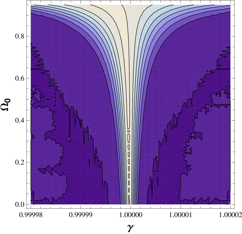
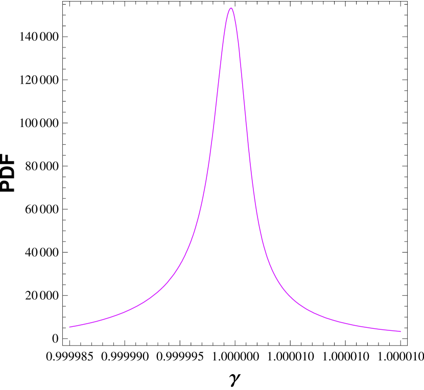
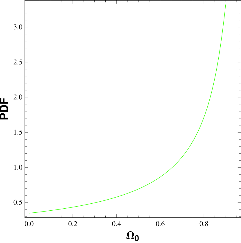
Figure 1: On the left, the two-dimensional probability distribution function (PDF) for the matter density $\Omega_{0}$ and the $\gamma$ parameter. In the center the one-dimensional PDF for the $\gamma$ parameter, and on the right the one-dimensional PDF for the matter density parameter $\Omega_{0}$.

IV Perturbative analysis: the scalar field description

The result described above is restricted to a fluid formulation of both components, that representing matter and that representing the exotic fluid. This exotic fluid must, more precisely, be represented by a field than a fluid - it is very difficult that a usual fluid could present the exotic behaviours connected with dark matter and dark energy, or even follow the new conservation law dictated by the Rastall’s theory. In this sense, let us consider the most simple field description in cosmology, that of a self-interacting scalar field. The energy momentum tensor of this field is given by,

$$T_{\mu\nu}=\phi_{;\mu}\phi_{;\nu}-\frac{1}{2}g_{\mu\nu}\phi^{;\rho}\phi_{;\rho}+g_{\mu\nu}V(\phi).$$ (39)

If we impose the usual conservation law for the energy-momentum tensor ${T^{\mu\nu}}_{;\mu}=0$, we obtain the usual Klein-Gordon equation:

$$\nabla_{\rho}\nabla^{\rho}\phi=-V_{\phi}(\phi).$$ (40)

However, if now the conservation law must read as in equation (7), the scalar field must now obey the following equation:

$$\nabla_{\rho}\nabla^{\rho}\phi+(3-2\gamma)V_{\phi}=(1-\gamma)\frac{\phi^{;\rho}\phi^{;\sigma}\phi_{;\rho;\sigma}}{\phi_{;\alpha}\phi^{;\alpha}}.$$ (41)

In the two fluid model, the corresponding “Einstein’s” equation takes the form,

$$R_{\mu\nu}-\frac{1}{2}g_{\mu\nu}R=\phi_{;\mu}\phi_{;\nu}-\frac{2-\gamma}{2}g_{\mu\nu}\phi_{;\rho}\phi^{;\rho}+g_{\mu\nu}(3-2\gamma)V(\phi).$$ (42)

From the scalar field description it comes out some similarities of the Rastall’s theory with the K-Essency models mukhanov . K-Essence models may also be plagued with negative sound velocity problems what strength the mentioned similarities linder .

One clear advantage in using the scalar field representation is that it usually avoids the problems of the fluid representation of components with negative pressure. However, while this is clear in the usual case, with the Einstein’s equation coupled to the ordinary Klein-Gordon’s equation, this is less clear in the framework of the Rastall’s theory. In order to investigate the constraints from mass power spectrum for this field formulation of the Rastall’s theory, we take the coupled system matter+scalar field+Rastall’s gravity, written in a convenient way for the perturbative analysis in the synchronous coordinate condition:

$$R_{\mu\nu} = \phi_{;\mu}\phi_{;\nu}+\frac{1-\gamma}{2}g_{\mu\nu}\phi_{;\rho}\phi^{;\rho}-(3-2\gamma)g_{\mu\nu}V+8\pi G\biggr{(}T_{\mu\nu}-\frac{1}{2}g_{\mu\nu}T\biggl{)},$$ (43)

$$\nabla_{\rho}\nabla^{\rho}\phi = -(3-2\gamma)V_{\phi}+(1-\gamma)\frac{\phi^{;\rho}\phi^{;\sigma}\phi_{;\rho;\sigma}}{\phi_{;\alpha}\phi^{;\alpha}},$$ (44)

$${T^{\mu\nu}}_{;\mu} = 0.$$ (45)

Now, let us suppose that the scalar field has zero pressure. Since the energy and the pressure of the scalar field is given by

$$\rho_{\phi} = \frac{\dot{\phi}^{2}}{2}+V(\phi),$$ (46)

$$p_{\phi} = \frac{\dot{\phi}^{2}}{2}-V(\phi),$$ (47)

the condition of zero pressure implies $\dot{\phi}^{2}/2=V$, leading to $\rho_{\phi}=\dot{\phi}^{2}$. From the point of view of the background, there is no difference between the fluid and scalar field approach. But at perturbative level the difference is significative.

In the synchronous coordinate condition, the perturbed equations corresponding to the system described by (43-45), are the following:

$$\ddot{\delta}+2\frac{\dot{a}}{a}\dot{\delta}-\frac{3}{2}\frac{\Omega_{0}}{a^{3}}\delta = (3-\gamma)\dot{\phi}\dot{\Psi}-(3-2\gamma)V_{\phi}\Psi,$$ (48)

$$\gamma\ddot{\Psi}+3\frac{\dot{a}}{a}\dot{\Psi}+\biggr{\{}\frac{k^{2}}{a^{2}}+(3-2\gamma)V_{\phi\phi}\biggl{\}}\Psi = \dot{\phi}\dot{\delta},$$ (49)

where $\Psi=\delta\phi$ and $\delta$ is the density contrast of the matter component. Using now the scale factor as the variable, the above system of equations take the following form:

$$\delta^{\prime\prime}+\biggr{\{}\frac{2}{a}+\frac{f^{\prime}(a)}{f(a)}\biggl{\}}\dot{\delta}-\frac{3}{2}\frac{\Omega_{0}}{a^{3}f^{2}(a)}\delta = (3-\gamma)\phi^{\prime}\Psi^{\prime}-(3-2\gamma)\frac{V_{\phi}}{f^{2}(a)}\Psi,$$ (50)

$$\gamma\Psi^{\prime\prime}+\biggr{\{}\frac{3}{a}+\gamma\frac{f^{\prime}(a)}{f(a)}\biggl{\}}\Psi^{\prime}+\biggr{\{}\frac{k^{2}}{a^{2}f^{2}(a)}+(3-2\gamma)\frac{V_{\phi\phi}}{f^{2}(a)}\biggl{\}}\Psi = \phi^{\prime}\delta^{\prime},$$ (51)

where

$$\phi^{\prime} = \sqrt{3\Omega_{x0}}\frac{a^{\frac{-3}{3-\gamma}}}{f(a)},$$ (52)

$$V = \frac{3}{2}\Omega_{x0}a^{\frac{-6}{3-\gamma}},$$ (53)

$$V_{\phi} = \frac{V_{a}}{\phi^{\prime}},$$ (54)

$$V_{\phi\phi} = \frac{1}{\phi^{\prime}}\frac{d}{da}V_{\phi}.$$ (55)

The function $f(a)$ is defined as before.

We perform the same statistical analysis as before, again imposing the initial conditions using the BBKS transfer function. The results are shown in figure 2. The main difference is that there is now two relevant regions in the space parameter: one around $\gamma=1$, with a low density, and the other near $\gamma=0$, but positive, extending from the low to high density. The region around $\gamma=1$ has high probabilities, but it is smaller; the region near $\gamma=0$ has lower probabilities, but extend to a large region. The consequence is that, after marginalization, there is two peaks in the one-dimensional probability for $\gamma$: one near $\gamma=1$ and another near $\gamma=0$. The second peak is higher. We think that this is an effect of the larger probability region around $\gamma=0$, which seems to compensate the higher probabilities around $\gamma=1$. There are also two peaks in the one-dimensional PDF for $\Omega_{0}$, one near $\Omega_{0}=0$ and another near $\Omega_{0}=1$. The best fitting is achieved for $\gamma=1.02$ and $\Omega_{0}=0.72$ with a $\chi^{2}$ per degree of freedom equal $0.30$ better than the $\Lambda$CDM model. The PDF goes quickly to zero for $\gamma<0$. Still concerning the peak near $\gamma=0$, the parameters for $\gamma$ and $\Omega_{0}$ in this region implies a $\chi^{2}$ around 0.33, high compared with the $\chi^{2}$ for $\gamma\sim 1$, but smaller than the $\Lambda$CDM best fitting. We may ask about the statistical relevance of this second peak.

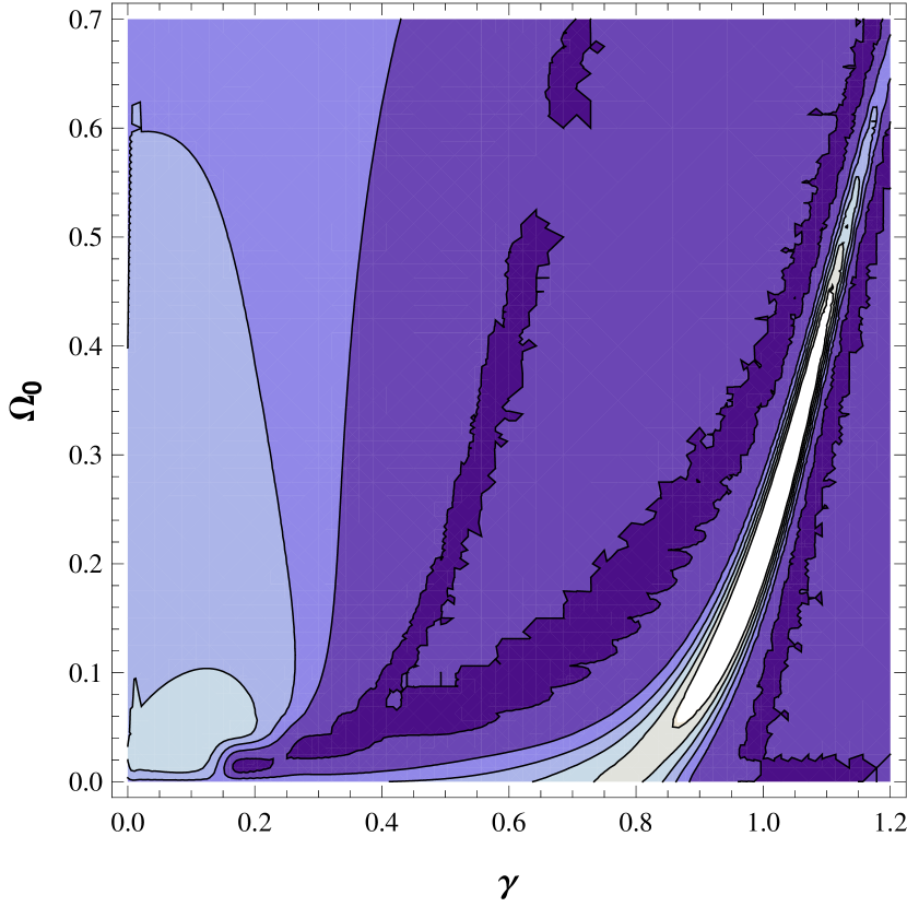
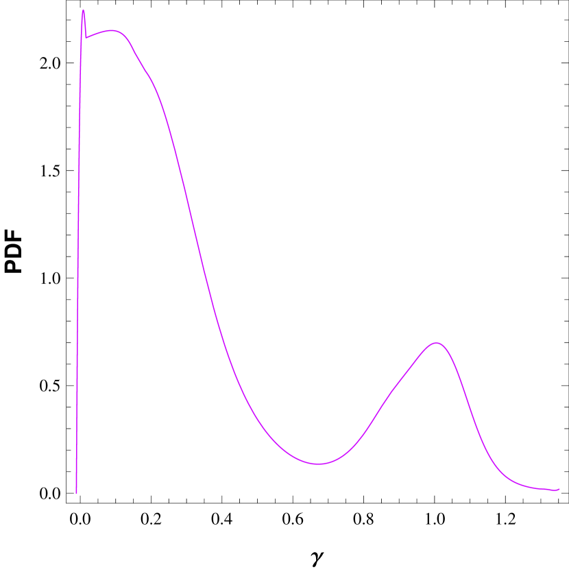
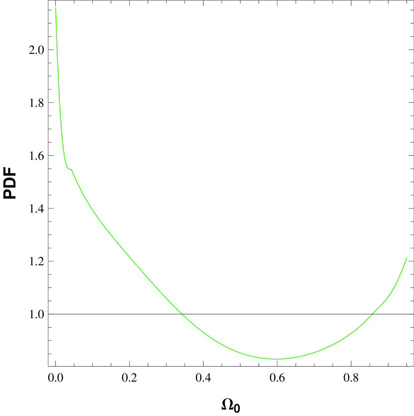
Figure 2: On the left, the two-dimensional probability distribution function (PDF) for the matter density $\Omega_{0}$ and the $\gamma$ parameter. In the center the one-dimensional PDF for the $\gamma$ parameter, and on the right the one-dimensional PDF for the matter density parameter $\Omega_{0}$.

V Conclusions

In this work we have investigate the Rastall’s proposal of modification of General Relativity with respect to the problem of structure formation. This proposal is equivalent to change the usual conservation law of General Relativity. In some sense, it can be seen as a modification of the equation of state of a given fluid from the dynamical point of view. In this sense, the Rastall’s theory can be interesting in order to obtain an accelerated expansion of the universe without introducing exotic fluids. For example fluids with positive or null pressure may induce a dynamics typical of fluids of negative pressure. This behaviour has already been remarked, for example, in the Brans-Dicke theory rose .

Our results indicate that the Rastall’s theory faces many problems at perturbative level. Considering a homogenous and isotropic universe for example, the effective equation of state of the background is entirely reproduced at perturbative level, leading to high instabilities when this effective equation of state implies negative pressure. One way out is to consider a two-fluid model, one of the fluids obeying the usual conservation law and the other one following the Rastall’s prescription. The results point out to a configuration which still reduces the Rastall’s theory to General Relativity.

When we keep the framework of two components which obeys different conservation laws, but with a self-interacting scalar field playing the role of the “Rastall’s fluid”, more interesting features appear. In particular, the Rastall’s proposal can be seen as a modification of the Klein-Gordon equation, similarly to what happens in the K-Essence theories mukhanov . Again the configuration corresponding to General Relativity is favored, but other configurations with $\gamma\sim 0$ are also possible even if some statistical subtleties appear. All these considerations seem to indicate to the specificity of General Relativity and rule out the Rastall’s theory.

A possible way out to save the Rastall’s proposal is to consider the modification of the usual conservation law as a manifestation of quantum effects (like particle production) in the spirit of reference ademir . The particle production in an expanding universe may lead to new terms in the usual conservation law. Such possibility remains to explore. In any case, it seems clear that structure formation asks for a fluid we behaves in the background and at perturbative level with zero effective pressure (otherwise no mass agglomeration can effectively occur), and this poses a serious problem in the original framework of the Rastall’s theory. In some sense, this has already been remarked in reference capone , forcing the authors of that work to use just one fluid to fit the supernova type Ia data. But, such procedure seems to be impossible concerning the structure formation problem.

Other observational methods, like CMB, may be used to constrain better the Rastall’s theory. But, the results obtained in the present work seem to us to be strong enough to point out the difficulties that the Rastall’s theory face when confronted with observational data.

Acknowledgements: We thank Oliver Piattela, Winfried Zimdahl and Hermano Velten for their remarks and criticisms on the text. We thank also CNPq (Brazil) and FAPES (Brazil) for partial financial support.

References

- (1) R.R. Caldwell and M. Kamionkowski, Ann. Rev. Nucl. Part. Sci. 59, 397(2009).
- (2) A. de Felice and S. Tsujikawa, f(R) theories, arXiv:1002.4928.
- (3) M. Capone, V.F. Cardone and M.L. Ruggiero, Accelerating cosmology in Rastall’s theory, arXiv:0906.4139.
- (4) P. Rastall, Phys. Rev. D6, 3357 (1972).
- (5) L.L. Samley, Class. Quant. Grav. 10, 1179 (1993).
- (6) L. Lindblom and W.A. Hiscock, J. Phys. A, 1827(1982).
- (7) J.C. Fabris, R. Kerner and J. Tossa, Int. J. Mod. Phys. D9, 111(2000).
- (8) J.C. Fabris and J. Martin, Phys. Rev.D55, 5205(1997).
- (9) S. Cole et al, Mon. Not. Roy. Astron. Soc. 362, 505(2005).
- (10) N. Sugiyama, Astrophys. J.Suppl. 100, 281(1995).
- (11) J.M. Bardeen, J.R. Bond, N. Kaiser and A.S. Szalay, Astrophys. J. 304, 15(1986).
- (12) J.C. Fabris, I. Shapiro and J. Solà, JCAP 0702, 016(2007)
- (13) R. de Putter and E.V. Linder, Astropart. Phys. 28, 263(2007)
- (14) C. Armendariz-Picon, V.F. Mukhanov and P.J. Steinhardt, Phys. Rev. Lett. 85, 4438(2000).
- (15) A.B. Batista, J.C. Fabris and R. de Sá Ribeiro, Gen. Rel. Grav. 33, 1237(2001).
- (16) S.H. Pereira, C.H.G. Bessa and J.A.S. Lima, Quantized fields and gravitational particle creation in f(R) expanding universes, arXiv:0911.0622.