Measures for a Transdimensional Multiverse
Abstract
The multiverse/landscape paradigm that has emerged from eternal inflation and string theory, describes a large-scale multiverse populated by “pocket universes” which come in a huge variety of different types, including different dimensionalities. In order to make predictions in the multiverse, we need a probability measure. In landscapes, the scale factor cutoff measure has been previously shown to have a number of attractive properties. Here we consider possible generalizations of this measure to a transdimensional multiverse. We find that a straightforward extension of scale factor cutoff to the transdimensional case gives a measure that strongly disfavors large amounts of slow-roll inflation and predicts low values for the density parameter , in conflict with observations. A suitable generalization, which retains all the good properties of the original measure, is the “volume factor” cutoff, which regularizes the infinite spacetime volume using cutoff surfaces of constant volume expansion factor.
I Introduction
Eternal inflation and string theory both suggest that we live in a multiverse which is home to many different types of vacua Vilenkin:1983xq ; Linde:1986fd ; Bousso:2000xa ; KKLT ; Susskind . Many of these vacua are high-energy metastable states that can decay to lower-energy states through bubbles which nucleate and expand in the high-energy vacuum background CdL . Inverse transitions are also possible: bubbles of high-energy vacuum can nucleate in low-energy ones EWeinberg 111This is the so-called “recycling” process. In both cases, the radius of the bubbles asymptotically approaches the comoving horizon size in the parent vacuum at the moment of nucleation recycling .. Once the process of eternal inflation begins, an unbounded number of bubbles will be created, one within the other, of every possible type. In addition each bubble has infinite spacelike slices when described in the maximally symmetric FRW coordinate system, and thus infinite spatial volume. The multiverse spacetime therefore has an infinite number of observers of every possible type.
In order to make predictions, we need to be able to compare the numbers of different types of events that can occur in the multiverse. This is non-trivial because of the aforementioned infinities, and has become known as “the measure problem” MPreviews . A number of measure proposals have been developed LM ; LLM ; GBLL ; AV94 ; AV95 ; Linde06 ; Linde07 ; GTV ; pockets ; GSPVW ; ELM ; diamond ; censor ; Vanchurin07 ; Winitzki08 ; LVW ; DeSimone:2008bq ; BB2 ; Guthlec , and some have already been ruled out, as they either lead to paradoxes or yield predictions in conflict with observations. All these measures have been defined within the context of regular “equidimensional” eternal inflation: all parent and daughter vacua have the same dimensionality. However, in general we expect the string theory landscape to allow parent vacua to nucleate daughter vacua with different effective dimensionality Zelnikov . The purpose of the present work is to introduce a measure for a “transdimensional” multiverse.
One of the most attractive measure proposals is the scale factor cutoff measure or, for brevity, scale factor measure LM ; LLM ; GBLL ; AV94 ; AV95 . It does not suffer from any obvious problems and gives prediction for the cosmological constant in a good agreement with the data DeSimone:2008bq ; BB2 ; Guthlec . In this measure the infinite spacetime volume of the multiverse is regularized with a cutoff at surfaces of constant scale factor. More precisely, one chooses some initial spacelike hypersurface , where the scale factor is set to be equal to one, , and follows the congruence of timelike geodesics orthogonal to that surface until the scale factor reaches some specified value . In the -dimensional case, the scale factor is defined as
| (1) |
where is the volume expansion factor along the geodesics. Relative probabilities are calculated by counting the number of times a given event occurs in the finite spacetime volume spanned by the congruence, between the initial () and final () hypersurfaces, in the limit that the scale factor cutoff .
In this paper we consider possible extensions of the scale factor measure to a transdimensional landscape. Eq. (1) defining the scale factor can be generalized as
| (2) |
where is the number of expanding (non-compact) dimensions. As a straightforward extension of the scale factor measure, one can still use constant- surfaces as a cutoff. We will find, however, that this prescription leads to a problem: it strongly disfavors large amounts of slow-roll inflation inside bubbles and predicts low values of the density parameter , in conflict with observations.
An alternative prescription is to use constant volume factor surfaces, , for a cutoff. We shall call this the volume factor measure. In an equidimensional multiverse, a surface of constant scale factor is also a surface of constant volume factor. However, for transdimensional universes, different vacua generally have different values of , so constant scale factor and volume factor surfaces are not the same. We will find that the volume factor cutoff results in an expression for comparing relative probabilities that is analogous to that of the equidimensional scale factor measure and provides a natural framework in which to extend the successful features of the scale factor measure to transdimensional landscapes.
The rest of the paper is organized as follows: In Section II we review the scale factor measure and outline how it can be implemented using the rate (master) equation formalism in four spacetime dimensions. In Section III we review the spacetime structure of a transdimensional multiverse using the 6-dimensional Einstein-Maxwell theory as an example and generalize the master equation to the transdimensional case. This formalism is then applied in Section IV to investigate the properties of the transdimensional volume factor and scale factor measures. Our conclusions are briefly summarized and discussed in Section V.
II The scale factor measure in
In this section we shall review the key features of the scale factor measure as found in Refs. DeSimone:2008bq ; BB2 ; Guthlec .
The scale factor time is defined in terms of the expansion factor of the geodesics as
| (3) |
and is related to the proper time via
| (4) |
Here, is the local expansion rate of the geodesic congruence, which can be defined as the divergence of the four-velocity field of the congruence,
| (5) |
We start with a congruence of geodesics orthogonal to the initial spacelike hypersurface and allow them to expand until the local scale factor reaches a critical value corresponding to . This defines the cutoff hypersurface . The relative probability to make an observation of type or is given by the ratio of the number of times that each type of observation ( or ) occurs in the spacetime volume spanned by the congruence, in the limit that ,
| (6) |
An intuitive picture of the scale factor cutoff emerges when we think of the geodesic congruence as a sprinkling of test “dust” particles. Imagine that this dust has a uniform density on our initial hypersurface . As the universe expands, the dust density (in the dust rest frame) dilutes. The scale factor cutoff is then initiated when the density drops below a critical value. The scale factor time can be expressed in terms of the dust density as
| (7) |
We can also introduce the volume expansion factor and the corresponding “volume time”
| (8) |
In a multiverse this time is trivially related to the scale factor time,
| (9) |
The definition of the scale factor time in terms of a geodesic congruence encounters ambiguities in regions of structure formation, where geodesics decouple from the Hubble flow and eventually cross. In particular, Eq. (7) suggests that scale factor time comes to a halt in bound structures, like galaxies, while it continues to flow in the intergalactic space. It is not clear whether one ought to use this local definition of for the scale factor cutoff, or use some nonlocal time variable that is more closely related to the FRW scale factor. Possible ways of introducing such a variable have been discussed in Refs. BB2 ; BB1 . Here we shall assume that some such nonlocal procedure has been adopted, so that structure formation has little effect on the cutoff hypersurfaces.
The numbers of observations in Eq. (6) are proportional to appropriately regularized volumes occupied by the corresponding vacua. We shall now review how these volumes can be calculated using the master equation of eternal inflation.
II.1 The rate equation
The comoving volume fractions occupied by vacua of type on a constant scale factor time slice obeys the rate equation (also called the master equation) recycling ; GSPVW
| (10) |
Here, the first term on the right-hand side accounts for loss of comoving volume due to bubbles of type nucleating within those of type , and the second term reflects the increase of comoving volume due to nucleation of type- bubbles within type- bubbles.
The transition rate is defined as the probability per unit scale factor time for a geodesic ”observer” who is currently in vacuum to find itself in vacuum ,
| (11) |
where is the bubble nucleation rate per unit physical spacetime volume,
| (12) |
is the expansion rate and is the energy density in vacuum . The total transition rate out of vacuum is given by the sum
| (13) |
We distinguish between the recyclable, non-terminal vacua with , which are sites of eternal inflation and further bubble nucleation, and the non-recyclable, “terminal vacua”, for which . Then, by definition, when the index corresponds to a terminal vacuum.
Eq. (10) can be written in a vector form,
| (14) |
where and
| (15) |
The asymptotic solution of (14) at large has the form
| (16) |
Here, is a constant vector which has nonzero components only in terminal vacua. Any such vector is an eigenvector of the matrix with zero eigenvalue,
| (17) |
As shown in GSPVW , all other eigenvalues of have a negative real part, so the solution approaches a constant at late times. Moreover, the eigenvalue with the smallest (by magnitude) real part is purely real. We have denoted this eigenvalue by and the corresponding eigenvector by .
The asymptotic values of the terminal components depend on the choice of initial conditions. For any physical choice, we should have . It can also be shown GSPVW that for terminal vacua and for recycling vacua. In the case of recycling vacua, it follows from Eq. (16) that
| (18) |
The physical properties of bubble interiors, such as the spectrum of density perturbations, the density parameter, etc., depend not only on the vacuum inside the bubble, but also on the parent vacuum that it tunneled from (or, more precisely, on the properties of the bubble implementing the transition between the two vacua). Bubbles should therefore be labeled by two indices, , referring to the daughter and parent vacua respectively. The fraction of comoving volume in type- bubbles, , satisfies a slightly modified rate equation Aguirre
| (19) |
Here and below we do not assume summation over repeated indices, unless the summation is indicated explicitely. The fractions and are related by
| (20) |
and the original rate equation (10) can be recovered from (19) by summation over . Solutions of Eq. (19) can also be expressed in the form (16), and for non-terminal bubbles we have
| (21) |
Note that it follows from (20) that the eigenvalue for the modified equation (19) should be the same as for the original equation.
The comoving volume fractions found on equal scale factor time hypersurfaces are directly related to the physical volume fractions. Thus we find that asymptotically the physical volumes in nonterminal bubbles are given by
| (22) |
where is the volume of the initial hypersurface and is the volume expansion factor. Note that the growth of volume is given by , where
| (23) |
is the fractal dimension of the inflating region Aryal . This is slightly less than , because volume is lost to terminal vacua.
Assuming that upward transitions in the landscape are strongly suppressed, the eigenvalue can be approximated as SchwartzPerlov:2006hi , where is the decay rate of the slowest-decaying vacuum. In general, it can be shown BB1 that
| (24) |
In the string theory landscape, is expected to be extremely small, and thus is very close to 3.
The volume fractions can also be expressed in terms of the volume time , which in our case is simply ,
| (25) |
where we have defined
| (26) |
and
| (27) |
II.2 The number of observers
Bubble interiors can be described by open FRW coordinates ,
| (28) |
where the functional form of is generally different in different bubbles. We shall assume for simplicity that all observers in bubbles of type are formed at a fixed FRW time with some average density . This defines the “observation hypersurface” within each habitable bubble. The infinite three-volume of this hypersurface is regularized by the scale factor cutoff at some . The regulated number of type- observers is
| (29) |
where is the total volume of observation hypersurfaces in all type- bubbles.
For our purposes in this paper, it will not be necessary to distinguish between the number of observers and the number of observations, so we shall use these terms interchangeably. If one is interested in some particular kind of observation, then in Eq. (29) should be understood as the density of observers who perform that kind of observation.
The calculation of the volume has been discussed in Refs. Vilenkin:1996ar ; BB2 ; Guthlec ; Bousso:2007nd . Here we give a simplified derivation, referring the reader to the original literature for a more careful analysis.
As the geodesics cross from the parent vacuum into the bubble, they become comoving with respect to the bubble FRW coordinates (28) within a few Hubble times. This implies that a fixed amount of FRW time roughly corresponds to a fixed amount of scale factor time along the geodesics. (This will be increasingly accurate at large .) We shall denote to be the amount of scale factor time between crossing into a bubble and reaching the observation hypersurface . If the expansion rate in the daughter bubble right after nucleation is not much different from the expansion rate in the parent vacuum, this can be approximated as
| (30) |
From Eq. (19), the comoving volume fraction that crosses into bubbles per time interval is
| (31) |
The corresponding physical volume is
| (32) |
where we have used Eq. (18) for the comoving volume fraction in the recycling parent vacuum . The total regulated volume of observation hypersurfaces in type- bubbles can now be expressed as
| (33) |
The factor in front of the integral accounts for volume expansion in bubble interiors, and the factor accounts for the volume loss due to bubble nucleation in the course of slow-roll inflation and subsequent non-vacuum evolution inside the bubbles. The corresponding nucleation rate is generally different from that in the vacuum; that is why we used a different notation. The integration in (33) is up to : regions added at later times are cut off before they evolve any observers. Performing the integration, we find
| (34) |
III A transdimensional multiverse
III.1 Einstein-Maxwell landscape
We now wish to generalize the above formalism to a transdimensional multiverse. We will try to keep the discussion general, but it will be helpful to have a specific model in mind. So we start by reviewing the Einstein-Maxwell model, which has been used as a toy model for flux compactification in string theory Douglas and has been recently studied in the multiverse context in Refs. BlancoPillado:2009di ; Carroll:2009dn ; BlancoPillado:2009mi .
The model includes Einstein’s gravity in dimensions, a Maxwell field, and a positive cosmological constant. It admits solutions in which some of the spatial dimensions are compactified on a sphere. These extra dimensions are stabilized by either magnetic or electric flux. The landscape of this theory has turned out to be unexpectedly rich. It includes a -dimensional de Sitter vacuum (), a variety of metastable -dimensional de Sitter and anti-de Sitter vacua ( and ) with two extra dimensions compactified on a -sphere (), and a number of vacua with four extra dimensions compactified on . The model also includes some perturbatively unstable and vacua (see also Krishnan:2005su ).
Quantum tunneling transitions between all these vacua have been discussed in Refs. BlancoPillado:2009di ; Carroll:2009dn ; BlancoPillado:2009mi . Transitions between different vacua (which were called “flux tunneling transitions” in BlancoPillado:2009di ) are similar to bubble nucleation in . They can be studied using the effective theory, where they are described by the usual Coleman-De Luccia formalism. From a higher-dimensional viewpoint, the compactified in the new vacuum inside the bubble has a different radius and a different magnetic flux. The role of the bubble walls is played by magnetically charged black -branes.
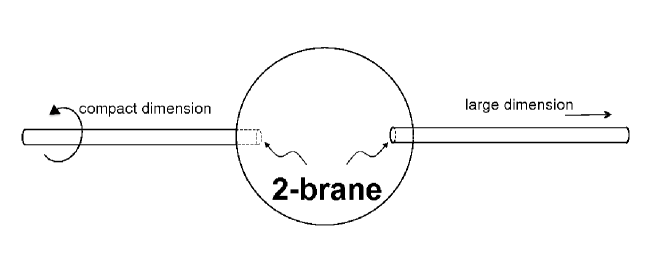
Another kind of transition occurs when the extra dimensions are destabilized in the new vacuum, so they start growing inside the bubble. The geometry resulting from such a decompactification transition, , is illustrated in Fig. 1. Observers in the parent vacuum see the nucleation and subsequent expansion of a bubble bounded by a spherical black -brane. The bubble interior is initially highly anisotropic, but as the compact dimensions expand, it approaches local isotropy, with the metric approaching that of a de Sitter space.
Transdimensional compactification transitions in which the parent vacuum has higher dimensionality than the daughter vacuum lead to a rather different spacetime structure Carroll:2009dn ; BlancoPillado:2009mi . Transitions from to occur through spontaneous nucleation of horizon-size spherical black branes, with the new compactified regions contained in the brane interiors. In transitions, the new regions are located inside spontaneously nucleated pairs of electrically charged black holes.
Transitions from to may also occur, but the corresponding instantons have not yet been identified. An additional vacuum decay channel, which can exist in more complicated models, is the nucleation of the so-called “bubbles of nothing” Witten ; I-Sheng ; Jose – that is, holes in spacetime bounded by higher-dimensional topological defects. In the case of flux compactification in , such bubbles can be formed if the Maxwell field is embedded into a gauge theory with a spontaneously broken non-Abelian symmetry Jose . The boundary defect then has codimension 3 and its cross-section has the form of a non-Abelian magnetic monopole.
III.2 Scale factor and volume factor times
The scale factor and volume factor times can be defined as before, in terms of a congruence of geodesics orthogonal to some initial hypersurface . The geodesics describe a dust of test particles which are initially uniformly spread over . (If has some compact dimensions, the particles are assumed to be uniformly spread both in large and compact dimensions.) The scale factor time is defined as
| (36) |
where is the proper time along geodesics, is given by
| (37) |
and is the effective number of spatial dimensions (that is, the number of non-compact dimensions) in the corresponding vacuum.
The volume factor time is related to as
| (38) |
As the geodesics flow into bubbles where some dimensions get decompactified or into black branes which have compactified regions in their interiors, the value of changes and with it the relation between and . Hence, in a transdimensional multiverse, equal scale factor hypersurfaces are not the same as equal volume factor hypersurfaces.
III.3 The rate equation
III.3.1 Scale factor time
Let us first consider the comoving volume rate equation using the scale factor time as our time variable. The form of the rate equation is the same as in the equidimensional case,
| (39) |
Here, is the comoving volume fraction in regions of type (which is proportional to the number of the geodesic “dust” particles in such regions) and is the probability per unit scale factor time for a geodesic which is currently in vacuum to cross into vacuum . The effect of bubble or black brane nucleation is to remove some comoving volume from the parent vacuum and add it to the daughter vacuum (except for the bubbles of nothing, where the excised comoving volume is lost). As in the case, the asymptotic radius of black branes and bubbles is equal to the comoving horizon size. This asymptotic value is approached very quickly, essentially in one Hubble time, and since the rate equation should be understood in the sense of coarse-graining over a Hubble scale, we can say it is reached instantly. The transition rates are given by
| (40) |
where is the effective number of dimensions in the parent vacuum and is a geometric factor. For flux tunneling bubbles, decompactification bubbles, and bubbles of nothing, the entire horizon region is excised, and is the volume inside a unit sphere in dimensions,222A similar transdimensional rate equation, but with somewhat different transition coefficients was presented by Carroll et.al in Ref. Carroll:2009dn . In particular, they made no distinction between the geometric factors for compactification and decompactification transitions.
| (41) |
We note that is the bubble (or black brane) nucleation rate in the large dimensions, so that is dimensionless.
In the case of compactification transitions, the geometric factor is different. Consider, for example, transitions in our Einstein-Maxwell model. These transitions occur through nucleation of electrically charged black holes, which are described by 6-dimensional Reissner-Nordstrom-de Sitter solutions,
| (42) |
where
| (43) |
Here, is the expansion rate of and the parameters and are proportional to the black hole mass and charge, respectively. The requirement that the instanton describing black hole nucleation should be non-singular imposes a relation between , and . In the limit when the black hole is much smaller than the cosmological horizon,
| (44) |
it can be shown BlancoPillado:2009mi that the black holes are nearly extreme, , with a Schwarzschild radius .
Dust particles initially at rest in the metric (42) exhibit two types of behavior. For sufficiently small values of , particles are captured by the black hole, while for they are driven away from the black hole by the cosmological expansion. The critical value can be found from
| (45) |
In the limit (44), we have
| (46) |
With , the geometric factor is
| (47) |
This expression is not exact, since comoving geodesics in the parent vacuum will not be at rest in the coordinates (42), but it will give a good approximation when (44) is satisfied.
In the case of transitions, the metric of nucleating black branes is
| (48) |
The functions and are not known analytically, but have been found numerically in Ref. BlancoPillado:2009mi . Once again, the critical radius below which the geodesics are captured by the brane can be found from the condition
| (49) |
and in the limit of we have
| (50) |
Here, the first factor comes from the area of the horizon-size 2-brane, and the second factor is the fraction of the horizon volume occupied by the captured particles in the three dimensions transverse to the brane333 We note that it follows from the analysis in Ref.’s Carroll:2009dn ; BlancoPillado:2009mi that in order to have a positive-energy vacuum inside the nucleated black brane, the magnetic charge of the brane should be of the order . This implies that the black brane and cosmological horizons are comparable to one another, and therefore . Hence, in this case the geometric factor is . .
One complication of the transdimensional case is that the volumes occupied by different regions are no longer simply related to the comoving volume fraction . The reason is that a given geodesic generally crosses regions with different values of and is thus exposed to different expansion rates at different times in its history. The rate equation for the physical volumes on the constant- surfaces can be written as 444Eq. (51) assumes that transitions between different vacua occur with conservation of volume, so the total volume is changed only due to cosmological expansion and due to volume loss to terminal bubbles. This would be so for a continuous evolution of the geodesic congruence, but is not obviously true for quantum transitions between the vacua. This issue requires further study. Here we note that accounting for a possible discontinuous volume change in the course of transitions could introduce an additional factor multiplying in (51). This would result in a renormalization of and would not change our general conclusions.
| (51) |
where we remind the reader that is the total decay rate out of vacuum , is the physical volume fraction of type vacua, reached from all possible type parent vacua, and is simply the number of large inflating directions in vacuum . Here, the volumes should be understood in the higher-dimensional sense, that is, including both large and compact dimensions. With the ansatz
| (52) |
this can be rewritten as
| (53) |
where
| (54) |
The right-hand side of (53) must be positive, since for inflating vacua. If is also an inflating vacuum, we should have and
| (55) |
Now, if we define
| (56) |
where is the largest dimension of an inflating vacuum in the landscape, then
| (57) |
The bound in Eq. (57) must be satisfied for all type vacua. The tightest constraint occurs when , from which it follows that555This derivation of Eq. (58) follows closely the derivation of Eq. (24) in Ref. BB1 .
| (58) |
where is the smallest decay rate among the vacua of effective dimension . As before, we expect to be very small, and thus
| (59) |
III.3.2 Volume factor time
The volume-factor-time rate equation can be written as
| (60) |
where the transition rates per unit time are given by
| (61) |
The asymptotic solution of this equation for non-terminal bubbles is
| (62) |
where is the smallest (by magnitude) eigenvalue of the matrix
| (63) |
Substitution of (62) into (60) gives the relation
| (64) |
and it follows, since the right hand side of (64) must be positive, that is smaller than the decay rate per unit volume factor time of any inflating vacuum,
| (65) |
Unlike the scale factor case, the volumes occupied by different vacua on the constant- surfaces are simply related to the comoving volume fractions,
| (66) |
where
| (67) |
III.4 The number of observers
III.4.1 Scale factor cutoff
The number of observers can now be evaluated along the same lines as in Section IIB. For the scale factor cutoff, the rate of volume increase in type- bubbles due to new bubble formation is
| (68) |
and the total volume of “observation hypersurfaces” in bubbles is given by
| (69) | |||
| (70) |
Dropping irrelevant constant factors, multiplying by the density of observers and using Eq. (56), we obtain for the total number of observers
| (71) |
Note that here the density should be understood in a higher-dimensional sense, so that , where is the volume of compact dimensions in vacuum .
III.4.2 Volume factor cutoff
Similarly, for the volume factor cutoff we find
| (72) |
| (73) | |||
| (74) |
and finally
| (75) |
Here,
| (76) |
and
| (77) |
is the volume factor time it takes for observers to evolve in type- bubbles.
IV Properties of scale factor and volume factor measures
IV.1 Number of e-folds of inflation and the density parameter
Suppose we have a landscape which includes bubbles (or black branes) with comparable nucleation rates and similar post-inflationary evolution, but different inflaton potentials. The bubbles then have different numbers of e-folds of slow-roll inflation and different values for the density parameter (measured at the same value of the CMB temperature, ).666The primordial density contrast will also generally vary. To simplify the analysis, here we consider only the section of the landscape where is fixed to its observed value in our part of the universe. We have verified, using some simple models, that inclusion of variation of does not significantly alter our conclusions. We want to investigate the effect of these differences on the number of observers, , regulated with scale factor and volume factor cutoffs.
The scale factor time , which appears in Eq. (71) for the number of observers, can be expressed as
| (78) |
where is the time it takes for observers to evolve after the end of inflation. The dependence of on the number of inflationary e-folds can now be read off from Eqs. (71), (78),
| (79) |
For an equidimensional landscape with , Eq.(79) gives
| (80) |
Since and are both extremely small, there is no selection effect favoring small or large values of DeSimone:2008bq ; DeSimone:2009dq . What has happened here is that there has been an almost precise cancellation of two effects: the volume growth inside bubbles, and the decrease in the number of nucleated bubbles as we go back in time.
Apart from the explicit dependence on shown in Eq. (79), also depends on through the anthropic factor and through the “prior” distribution
| (81) |
Since a long slow-roll inflation requires fine-tuning, one can expect that is a decreasing function of . Analysis of a simple landscape model in Ref. FKRS suggests a power-law dependence,
| (82) |
with .
The dependence of the anthropic factor on has been discussed in Refs. GTV ; FKRS ; DeSimone:2009dq . This dependence is more conveniently expressed in terms of the density parameter , which is related to as
| (83) |
The value of the constant depends on the duration of the inflaton-dominated period, which may occur between the end of inflation and the onset of thermalization, and on the thermalization temperature . Assuming instant thermalization at a GUT-scale temperature , we have . In the opposite extreme of low thermalization temperature, , .
The anthropic significance of is due to its effect on structure formation. For very close to 1, , this effect is negligible. For significantly less than 1, the growth of density perturbations terminates at redshift . For this strongly interferes with structure formation. The density of galaxies, and the density of observers, decreases somewhat with in the range and drops rapidly towards zero at DeSimone:2009dq . This behavior can be roughly accounted for by imposing a sharp cutoff at . Using Eq. (83), this translates into a cutoff on at . The density of observers then effectively becomes a step function,
| (84) |
With the prior from Eq.(82), the full distribution for is given by
| (85) |
where the prefactor is chosen so that the distribution is normalized to 1.
Observations indicate that in our part of the universe , which corresponds to
| (86) |
According to (85), the probability of this observation is
| (87) |
Since in Eq. (86) is only slightly greater than , this probability is close to 1, as long as is not very large (which is certainly the case for ). Hence, the observed value of is fully consistent with the equidimensional scale factor measure DeSimone:2009dq .
The situation is very different in a transdimensional landscape. Omitting the exponentially small terms in the exponent of Eq. (79), we have
| (88) |
This shows that large amounts of slow-roll inflation are strongly disfavored in all bubbles with . For example, in the case of -dimensional bubbles or branes in our Einstein-Maxwell theory , . In string theory landscape, we could have and an even stronger suppression, .
The reason is as follows: bubbles which undergo less e-folds of inflation before being able to produce observers get rewarded by being more plentiful, but undergo less expansion than other bubbles which have a longer “gestation” period. These are the same two competing effects we discussed above for regular inflation. The difference here, in the transdimensional case, is that the internal volume reward (which grows like ) is not enough to compensate for the lower number of bubbles which nucleate at earlier times ().
Using Eq. (84) for and disregarding the power-law prior compared to the steep dependence on in (88), we obtain
| (89) |
The probability for the observed bound on is then
| (90) |
where we have set and used Eq. (86) in the last step. For , this probability is smaller than , so the transdimensional scale factor measure can be ruled out at a high confidence level.
Turning now to the volume factor measure, we have from Eqs. (78),(77)
| (91) |
and Eq. (75) for the number of observers gives
| (92) |
This is essentially the same as Eq.(80). There is no strong selection for large or small values of , so the same analysis as we gave above for the equidimensional case should apply here. Thus, we conclude that the transdimensional volume factor measure is consistent with observations of .
IV.2 Youngness bias
Another pitfall that a candidate measure needs to avoid is the “youngness paradox” LLM95 ; Guth00 . Consider two kinds of observers who live in the same type of bubbles, but take different time to evolve after the end of inflation. Observers who take less time to evolve can live in bubbles that nucleate closer to the cutoff and thus have more volume available to them. With proper time slicing, this growth of volume is so fast that observers evolving even a tiny bit faster are rewarded by a huge volume factor, resulting in some bizarre predictions LLM95 ; Guth00 ; Tegmark ; Bousso:2007nd . On the other hand, the scale factor cutoff in gives only a mild youngness bias DeSimone:2008bq ,
| (93) |
so observers evolving faster by a scale factor time are rewarded by a bias factor
| (94) |
The generalization of Eqs. (93) and (94) to a transdimensional landscape can be read off from Eq. (71):
| (95) |
and
| (96) |
Note that here, and in Eq.(93) above, we omitted the factor which accounts for the growth of volume inside bubbles in the time interval . The reason is that post-inflationary expansion only dilutes matter (e.g., galaxies) and does not by itself result in any increase in the number of observers.777This means that the density of observers that we used in the preceding sections should be . This relation accounts only for dilution of galaxies with cosmic time, but in fact some new galaxies will also be formed, so the dependence of on will be more complicated. This effect is unimportant in the context of the youngness paradox, so we disregard it here. In string theory landscape we could have , so the youngness bias (96) is stronger than in the equidimensional case, but it is still mild enough to avoid any paradoxes.
Similarly, for the transdimensional volume factor cutoff we have
| (97) |
and
| (98) |
For -dimensional regions this gives , the same as in the equidimensional case.
IV.3 Boltzmann brains
Yet another potential problem for the measure is an excessive production of Boltzmann brains (BBs) – freak observers spontaneously nucleating as de Sitter vacuum fluctuations Rees1 ; DKS02 ; Albrecht ; Page1 ; Page06 ; BF06 . Measures predicting that BBs greatly outnumber ordinary observers should be ruled out.
The total number of BBs nucleated in type- bubbles can be estimated as
| (99) |
where is the total spacetime volume in such bubbles and is the BB nucleation rate. Here we disregard possible time variation of the nucleation rate during the early evolution in bubble interiors. The bulk of BB production tends to occur at late stages, after vacuum domination. The nucleation rate is then constant and depends only on the vacuum inside the bubble, not on the parent vacuum.
The spacetime volume can be found by integrating the spatial volume over the proper time . With a scale factor cutoff, we find
| (100) |
with from Eq. (56). Combining this with Eqs. (99) and (71), we obtain for the relative number of BBs and normal observers
| (101) | |||
| (102) |
where
| (103) |
is the dimensionless BB nucleation rate and we have used Eq. (53) in the last step.
In an equidimensional landscape with , Eq. (102) gives
| (104) |
The rate of BB nucleation is extremely small, with estimates ranging from to BB1 ; BB2 . Compared to this, most quantities which can be large or small by ordinary standards, can be regarded as . In particular, this applies to the number of observers per horizon volume, BB1 ; BB2 . Hence,
| (105) |
so BB domination in vacuum is avoided only if the vacuum decay rate is greater than the BB nucleation rate,
| (106) |
In particular, this condition should be satisfied by our vacuum Linde06 .
Even if ordinary observers can evolve only in our vacuum, BBs might be able to nucleate in other vacua as well. For example, vacua having the same low-energy physics and differ from ours only by the value of the cosmological constant can nucleate human-like observers, as long as is small enough, so that the observers are not torn apart by the gravitational tidal forces. General conditions for the avoidance of BB domination have been discussed in Refs. BB1 ; BB2 . The main condition is that Eq. (106) should be satisfied for any vacuum that can support Boltzmann brains. This is a rather non-trivial condition. Vacuum decay rates can be extremely low, especially for vacua with a low supersymmetry breaking scale. Hence, the equidimensional scale factor measure may or may not be consistent with observations, depending on the details of the landscape.
In the transdimensional case, for vacua with , Eq. (102) gives
| (107) |
where, following BB1 ; BB2 , we have set . Thus, the Boltzmann brain problem of the scale factor measure disappears in the transdimensional case, even if it existed in the equidimensional landscape.
For the volume factor cutoff, Eqs. (100) and (102) are replaced by
| (108) |
and
| (109) |
This is essentially the same as Eq. (105) for the equidimensional scale factor measure. Hence, we expect the conditions for BB avoidance in a transdimensional landscape with a volume factor cutoff to be the same as derived in BB1 ; BB2 for the scale factor measure in .
V Conclusions
In this paper we investigated possible generalizations of the scale factor measure to a transdimensional multiverse. We considered two such generalizations: a straightforward extension of the scale factor cutoff and the volume factor cutoff. Here we briefly summarize and discuss our results.
We found that the transdimensional scale factor measure is not subject to the youngness or Boltzmann brain paradoxes. One of the key features of this measure is that it exponentially disfavors large amounts of slow-roll inflation inside the bubbles. This results in preference for low values for the density parameter , while observations indicate that is actually very close to 1,
| (110) |
The severity of the problem depends on the highest dimension of an inflating vacuum in the landscape. The probability for the bound (110) to hold is
| (111) |
For this gives a reasonably large probability . If indeed we live in a multiverse with , then this measure makes a strong prediction that a negative curvature will be detected when the measurement accuracy is improved by another order of magnitude. On the other hand, if , as can be expected in string theory landscape, we have , and the scale factor measure is observationally ruled out at a high confidence level.
One potential pitfall for the measure that we have not discussed in the body of the paper is the runaway problem, also known as or catastrophe. This problem arises in measures that exponentially favor large amounts of inflationary expansion. The primordial density contrast and the gravitational constant are strongly correlated with the number of e-folds of inflation , and an exponential probability distribution for indicates that the distributions for and should also be very steep, driving their expected magnitudes to extreme values FHW ; QGV ; GS . These problems are often referred to as and “catastrophes”. In our case, large inflation is exponentially , and the situation is different. The runaway toward small values of is stopped by the anthropic bound on . The resulting prediction for may be too low, as described above. But if the distribution for is acceptable, as it could be for , then and catastrophes may also be avoided. This would happen if the distribution is cut off by the anthropic bound on before it gets into the dangerous range of or . (Note that is much more sensitive to the value of than or .)
The properties of the volume factor measure are essentially the same as those of the scale factor measure in dimensions. It is free from the and catastrophes and from the youngness paradox. It may or may not have a Boltzmann brain (BB) problem, depending on the properties of the landscape. The conditions for BB avoidance for this measure are the same as found in Refs. BB1 ; BB2 in the case, the main condition being that the rate of BB nucleation in any vacuum should be smaller than the decay rate of that vacuum. Whether or not this condition is satisfied in the string theory landscape is presently an open question. The answer depends both on the unknown properties of the landscape and on our understanding of what exactly constitutes a Boltzmann brain. In any case, at our present state of knowledge, the volume factor measure is certainly not ruled out by the BB problem.
Our goal in this paper was to analyze and compare the properties of the scale factor and volume factor measures in a transdimensional multiverse. Our results suggest that the volume factor cutoff is a more promising measure candidate. It avoids all potential measure problems, with the judgement still pending on the BB paradox. On the other hand, we found that the scale factor measure suffers from a serious problem, predicting low values for the density parameter . This problem becomes acceptably mild only if the highest dimension of the inflating vacua in the landscape is .
We note finally the recent work GV08 ; GV09 ; Fiol which used holographic ideas for motivating the scale factor measure in . The proposal is that the dynamics of an eternally inflating universe has a dual representation in the form of Euclidean field theory defined at future infinity. An ultraviolet cutoff in this boundary theory then corresponds to a scale factor cutoff in the bulk. It would be interesting to see whether or not these ideas can be extended to a transdimensional multiverse.
VI Acknowledgements
We are grateful to Jaume Garriga for discussions and some crucial suggestions. We also benefited from very helpful discussions with Jose Blanco-Pillado and Michael Salem. This work was supported in part by grant PHY-0855447 from the National Science Foundation and by grant RFP2-08-30 from the Foundational Questions Institute (fqxi.org).
References
- (1) A. Vilenkin, Phys. Rev. D 27, 2848 (1983).
- (2) A. D. Linde, “Eternally existing self-reproducing chaotic inflationary universe,” Phys. Lett. B 175, 395 (1986).
- (3) R. Bousso and J. Polchinski, “Quantization of four-form fluxes and dynamical neutralization of the cosmological constant,” JHEP 0006, 006 (2000).
- (4) S. Kachru, R. Kallosh, A. Linde and S. P. Trivedi, “De Sitter vacua in string theory,” Phys. Rev. D 68, 046005 (2003)
- (5) L. Susskind, “The anthropic landscape of string theory,” 2003 arXiv:hep-th/0302219.
- (6) S. R. Coleman and F. De Luccia, “Gravitational Effects On And Of Vacuum Decay,” Phys. Rev. D 21, 3305 (1980).
- (7) K. M. Lee and E. J. Weinberg, Phys. Rev. D 36, 1088 (1987).
- (8) J. Garriga and A. Vilenkin, Phys. Rev. D57, 2230 (1998).
- (9) For recent reviews of the measure problem, see e.g. S. Winitzki, “Predictions in eternal inflation,” Lect. Notes Phys. 738, 157 (2008) [arXiv:gr-qc/0612164]; A. H. Guth, Phys. Rept. 333, 555 (2000); “Eternal inflation and its implications,” J. Phys. A 40, 6811 (2007) [arXiv:hep-th/0702178]; A. Linde, “Inflationary Cosmology,” Lect. Notes Phys. 738, 1 (2008) [arXiv:0705.0164 [hep-th]]; A. Vilenkin, “A measure of the multiverse,” J. Phys. A 40, 6777 (2007) [arXiv:hep-th/0609193]; A. Aguirre, S. Gratton and M. C. Johnson, “Measures on transitions for cosmology from eternal inflation,” Phys. Rev. Lett. 98, 131301 (2007) [arXiv:hep-th/0612195].
- (10) A. D. Linde and A. Mezhlumian, “Stationary universe,” Phys. Lett. B 307, 25 (1993) [arXiv:gr-qc/9304015].
- (11) A. D. Linde, D. A. Linde and A. Mezhlumian, “From the Big Bang theory to the theory of a stationary universe,” Phys. Rev. D 49, 1783 (1994) [arXiv:gr-qc/9306035].
- (12) J. Garcia-Bellido, A. D. Linde and D. A. Linde, “Fluctuations of the gravitational constant in the inflationary Brans-Dicke cosmology,” Phys. Rev. D 50, 730 (1994) [arXiv:astro-ph/9312039]; J. Garcia-Bellido and A. D. Linde, “Stationarity of inflation and predictions of quantum cosmology,” Phys. Rev. D 51, 429 (1995) [arXiv:hep-th/9408023]; J. Garcia-Bellido and A. D. Linde, “Stationary solutions in Brans-Dicke stochastic inflationary cosmology,” Phys. Rev. D 52, 6730 (1995) [arXiv:gr-qc/9504022].
- (13) A. Vilenkin, “Predictions from quantum cosmology,” Phys. Rev. Lett. 74, 846 (1995) [arXiv:gr-qc/9406010].
- (14) A. Vilenkin, “Making predictions in eternally inflating universe,” Phys. Rev. D 52, 3365 (1995) [arXiv:gr-qc/9505031].
- (15) A. Linde, “Sinks in the Landscape, Boltzmann Brains, and the Cosmological Constant Problem,” JCAP 0701, 022 (2007) [arXiv:hep-th/0611043].
- (16) A. Linde, “Towards a gauge invariant volume-weighted probability measure for eternal inflation,” JCAP 0706, 017 (2007) [arXiv:0705.1160 [hep-th]].
- (17) J. Garriga, T. Tanaka and A. Vilenkin, “The density parameter and the Anthropic Principle,” Phys. Rev. D 60, 023501 (1999) [arXiv:astro-ph/9803268].
- (18) A. Vilenkin, “Unambiguous probabilities in an eternally inflating universe,” Phys. Rev. Lett. 81, 5501 (1998) [arXiv:hep-th/9806185]; V. Vanchurin, A. Vilenkin and S. Winitzki, “Predictability crisis in inflationary cosmology and its resolution,” Phys. Rev. D 61, 083507 (2000) [arXiv:gr-qc/9905097].
- (19) J. Garriga, D. Schwartz-Perlov, A. Vilenkin and S. Winitzki, “Probabilities in the inflationary multiverse,” JCAP 0601, 017 (2006) [arXiv:hep-th/0509184].
- (20) R. Easther, E. A. Lim and M. R. Martin, “Counting pockets with world lines in eternal inflation,” JCAP 0603, 016 (2006) [arXiv:astro-ph/0511233].
- (21) R. Bousso, “Holographic probabilities in eternal inflation,” Phys. Rev. Lett. 97, 191302 (2006) [arXiv:hep-th/0605263]; R. Bousso, B. Freivogel and I. S. Yang, “Eternal inflation: The inside story,” Phys. Rev. D 74, 103516 (2006) [arXiv:hep-th/0606114].
- (22) L. Susskind, “The Census Taker’s Hat,” arXiv:0710.1129 [hep-th].
- (23) V. Vanchurin, “Geodesic measures of the landscape,” Phys. Rev. D 75, 023524 (2007) [arXiv:hep-th/0612215].
- (24) S. Winitzki, “A volume-weighted measure for eternal inflation,” arXiv:0803.1300 [gr-qc].
- (25) A. Linde, V. Vanchurin and S. Winitzki, “Stationary Measure on a Multisuperspace,” to be published.
- (26) A. De Simone, A. H. Guth, M. P. Salem and A. Vilenkin, Phys. Rev. D 78, 063520 (2008) [arXiv:0805.2173 [hep-th]].
- (27) R. Bousso, B. Freivogel and I. S. Yang, “Properties of the scale factor measure,” Phys. Rev. D 79, 063513 (2009) [arXiv:0808.3770 [hep-th]].
- (28) A. Guth, “Scale factor cutoff and bubble geometry”, unpublished notes, 2008.
- (29) A.D. Linde and M.I. Zelnikov, Phys. Lett. B215, 59 (1988).
- (30) A. Aguirre, S. Gratton and M.C. Johnson, Phys. Rev. Lett. 98, 131301 (2007).
- (31) M. Aryal and A. Vilenkin, Phys. Lett. B199, 351 (1987).
- (32) D. Schwartz-Perlov and A. Vilenkin, JCAP 0606, 010 (2006) [arXiv:hep-th/0601162].
- (33) A. De Simone, A. H. Guth, A. Linde, M. Noorbala, M. P. Salem and A. Vilenkin, “Boltzmann brains and the scale-factor cutoff measure of the multiverse,” arXiv:0808.3778 [hep-th].
- (34) A. Vilenkin and S. Winitzki, Phys. Rev. D 55, 548 (1997) [arXiv:astro-ph/9605191].
- (35) R. Bousso, B. Freivogel and I. S. Yang, Phys. Rev. D 77, 103514 (2008) [arXiv:0712.3324 [hep-th]].
- (36) M.R. Douglas and S. Kachru, Rev. Mod. Phys. 79, 733 (2007).
- (37) J. J. Blanco-Pillado, D. Schwartz-Perlov and A. Vilenkin, JCAP 0912, 006 (2009) [arXiv:0904.3106 [hep-th]].
- (38) S. M. Carroll, M. C. Johnson and L. Randall, JHEP 0911, 094 (2009) [arXiv:0904.3115 [hep-th]].
- (39) J. J. Blanco-Pillado, D. Schwartz-Perlov and A. Vilenkin, arXiv:0912.4082 [hep-th].
- (40) C. Krishnan, S. Paban and M. Zanic, “Evolution of gravitationally unstable de Sitter compactifications,” JHEP 0505, 045 (2005) [arXiv:hep-th/0503025].
- (41) E. Witten, Nucl. Phys. B195, 481 (1982).
- (42) I.S. Yang, “Stretched extra dimensions and bubbles of nothing in a toy model landscape,” arXiv:0910.1397 [hep-th].
- (43) J.J. Blanco-Pillado and B. Shlaer, “Bubbles of nothing in flux compactifications,” arXiv:1002.4408 [hep-th].
- (44) A. De Simone and M. P. Salem, arXiv:0912.3783 [hep-th].
- (45) B. Freivogel, M. Kleban, M. Rodrigues Martinez and L. Susskind, JHEP 0603:039 (2006).
- (46) A.D. Linde, D.A. Linde and A. Mezhlumian, Phys. Lett. B 345, 203 (1995).
- (47) A.H. Guth, Phys. Rept. 333, 555 (2000).
- (48) M. Tegmark, JCAP 0504:001 (2005)
- (49) M. Rees, Before the Beginning, p.221 (Addison-Wesley, 1997).
- (50) L. Dyson, M. Kleban and L. Susskind, “Disturbing implications of a cosmological constant,” JHEP 0210, 011 (2002) [arXiv:hep-th/0208013].
- (51) A. Albrecht and L. Sorbo, “Can the universe afford inflation?,” Phys. Rev. D 70, 063528 (2004) [arXiv:hep-th/0405270];
- (52) D. N. Page, “The lifetime of the universe,” J. Korean Phys. Soc. 49, 711 (2006) [arXiv:hep-th/0510003].
- (53) D. N. Page, “Is our universe likely to decay within 20 billion years?,” arXiv:hep-th/0610079.
- (54) R. Bousso and B. Freivogel, “A paradox in the global description of the multiverse,” JHEP 0706, 018 (2007) [arXiv:hep-th/0610132].
- (55) B. Feldstein, L. J. Hall and T. Watari, “Density perturbations and the cosmological constant from inflationary landscapes,” Phys. Rev. D 72, 123506 (2005) [arXiv:hep-th/0506235];
- (56) J. Garriga and A. Vilenkin, “Anthropic prediction for Lambda and the Q catastrophe,” Prog. Theor. Phys. Suppl. 163, 245 (2006) [arXiv:hep-th/0508005].
- (57) M. L. Graesser and M. P. Salem, “The scale of gravity and the cosmological constant within a landscape,” Phys. Rev. D 76, 043506 (2007) [arXiv:astro-ph/0611694].
- (58) J. Garriga and A. Vilenkin, JCAP 0901:021 (2009)
- (59) J. Garriga and A. Vilenkin, “Holographic multiverse and conformal invariance”, arXiv:0905.1509 [hep-th].
- (60) B. Fiol, “Defect CFTs and holographic multiverse”, arXiv:1004.0618 [hep-th].