Hydrodynamics of rapidly rotating superfluid neutron stars with mutual friction

Abstract

We study time evolutions of superfluid neutron stars, focussing on the nature of the oscillation spectrum, the effect of mutual friction force on the oscillations and the hydrodynamical spin-up phase of pulsar glitches. We linearise the dynamical equations of a Newtonian two-fluid model for rapidly rotating backgrounds. In the axisymmetric equilibrium configurations, the two fluid components corotate and are in $\beta$-equilibrium. We use analytical equations of state that generate stratified and non-stratified stellar models, which enable us to study the coupling between the dynamical degrees of freedom of the system. By means of time evolutions of the linearised dynamical equations, we determine the spectrum of axisymmetric and non-axisymmetric oscillation modes, accounting for the contribution of the gravitational potential perturbations, i.e. without adopting the Cowling approximation. We study the mutual friction damping of the superfluid oscillations and consider the effects of the non-dissipative part of the mutual friction force on the mode frequencies. We also provide technical details and relevant tests for the hydrodynamical model of pulsar glitches discussed by Sidery, Passamonti & Andersson (2010). In particular, we describe the method used to generate the initial data that mimic the pre-glitch state, and derive the equations that are used to extract the gravitational-wave signal.

1 Introduction

Mature neutron stars are expected to have superfluid and superconducting components in their interior. Shortly after a neutron star’s birth the temperature decreases below $T\simeq 10^{9}~{}\rm{K}$, at which point superfluid neutrons should be present both in the inner crust and the outer core, while the core protons should form a superconductor. At all relevant temperatures, the electrons form a “normal” fluid that is tightly locked to the protons due to the electromagnetic interaction. This suggests that the dynamics of mature neutron stars depends on the detailed interaction between coupled superfluids-superconductors (Glampedakis, Andersson & Samuelsson, 2010), i.e. represents a complex physics problem. The situation is not expected to simplify if one also accounts for the inner neutron star core, at several times the nuclear saturation density, where exotic states like hyperon superfluid mixtures or deconfined quark condensates may be present.

Although it is generally appreciated that neutron stars have this very complicated structure, the evidence for the presence of the different superfluid phases remain indirect. The strongest support comes from observed pulsar glitches, rapid spin-up events seen in a number of young pulsars (and also some magnetars) during their magnetic slow-down phase. The typical glitch size is very small, representing a relative change ($\Delta\Omega$) in the observed rotation rate ($\Omega$) in the range $10^{-9}<\Delta\Omega/\Omega<10^{-5}$. The currently accepted model for these events relies on the transfer of angular momentum between a (faster spinning) superfluid neutron component and the star’s (slower spinning) elastic crust (to which the magnetic field is anchored). The exchange is thought to be mediated by neutron vortices (by means of which the superfluid mimics bulk rotation) and the associated mutual friction (Alpar et al., 1984).

A challenge for future observations is to probe the detailed physics of a neutron star’s interior. In this context, asteroseismology associated with either gravitational or electromagnetic signals seems particularly promising. In fact, the quasiperiodic oscillations seen in the tails of giant magnetar flares may have provided us with the first opportunity to test our theoretical models against observational data (see for instance Watts & Strohmayer, 2007, and references therein). The observed variability likely originates from crustal oscillations and depends on the detailed crust dynamics and the interaction with the neutron star’s magnetic field. These observations have led to a resurgence of interest in neutron-star seismology and a renewed assault on the problem of magnetic star oscillations, a seriously challenging problem from the theory point-of-view (see Colaiuda, Beyer & Kokkotas, 2009, for a discussion of the literature). In the context of the present paper, the potential relevance of the neutron superfluid that penetrates the neutron star crust is particularly relevant (Andersson, Glampedakis & Samuelsson, 2009; Samuelsson & Andersson, 2009). The prospect of detecting gravitational waves from oscillating neutron stars is also exciting, especially since the associated signals will allow us to probe the high-density region and hence the supranuclear equation of state (EoS) (Andersson & Kokkotas, 1998; Benhar, Ferrari & Gualtieri, 2004; Samuelsson & Andersson, 2007; Andersson et al., 2009).

In order to faciliate future observations and the decoding of collected data, we need to improve our models considerably. The superfluid aspects are particularly interesting in this respect, since the oscillation spectrum of a superfluid star is more complex than that of a single fluid model. In superfluid regions fluid elements can execute both co- and counter-moving motion, leading to the existence of unique “superfluid” oscillation modes. Our understanding of the nature of the additional degree(s) of freedom and the effect on observables must be improved by detailed modelling, ultimately in the context of general relativistic multi-fluid dynamics.

The present work presents recent progress towards this goal. We study the oscillations of superfluid neutron stars by evolving in time the linearized two-fluid equations in Newtonian gravity. We improve on the analysis of Passamonti et al. (2009a) by including the perturbations of the gravitational potential. We also account for the mutual friction force associated with vortices, and implement quadrupole extraction of the gravitational-wave signal associated with the fluid motion. We provide the detailed analysis (and relevant code tests) for the configurations that we recently used to study the hydrodynamics of pulsar glitches (Sidery et al., 2010). We consider two simple analytical EoS and construct two distinct sequences of rapidly rotating stars, the main difference being the presence or absence of composition gradients. Such gradients impact on the superfluid dynamics, as the co- and counter-moving degrees of freedom are coupled in stratified models. From time-evolutions of the relevant perturbation equations, with the gravitational potential perturbation included, we determine the axi- and non-axisymmetric oscillation modes for models that rotate up to the mass shedding limit. Finally, we account for the (standard form of the) mutual friction force. This adds two coupling terms to the equations of motion. One component is dissipative and damps an oscillation mode, while the other modifies the frequencies of the superfluid modes. We study both these effects and infer an analytical relation for the associated frequency change of the non-axisymmetric superfluid fundamental and inertial modes.

2 Equations of Motion

In a basic model for superfluid neutron stars, the matter constituents are superfluid neutrons, superconducting protons and normal electrons. Given the typical dynamical timescale of stellar oscillations, one would expect the charged particles to be efficiently locked together by the electromagnetic interaction. Therefore, the dynamics of superfluid stars depends on two components, a neutron superfluid and a neutral conglomerate of protons and electrons. For simplicity, we will refer to the latter mixture as the “protons” in the following. More detailed discussion and justification for the two-fluid model is provided by Mendell (1991a, b), Prix (2004) and Andersson & Comer (2006).

When the mass of each fluid component is conserved, i.e. when we neglect the various particle reactions, the dynamics of a superfluid star is described by two mass conservation laws, two Euler-type equations and the Poisson equation for the gravitational potential (Prix, 2004). These take the form;

$$\partial_{t}\rho_{\mathrm{x}}+\nabla_{i}\left(\rho_{\mathrm{x}}v_{\mathrm{x}}^{i}\right)=0\,,\\$$ (1)

$$\left(\partial_{t}+v_{\mathrm{x}}^{k}\nabla_{k}\right)\left(v_{i}^{\mathrm{x}}+\varepsilon_{\mathrm{x}}w_{i}^{\mathrm{y}\mathrm{x}}\right)+\nabla_{i}\left(\Phi+\tilde{\mu}_{\mathrm{x}}\right)+\varepsilon_{\mathrm{x}}w_{k}^{\mathrm{y}\mathrm{x}}\nabla_{i}v_{\mathrm{x}}^{k}=\frac{f^{\mathrm{x}}_{i}}{\rho_{\mathrm{x}}}\,,\\$$ (2)

$$\nabla^{2}\Phi=4\pi G\rho\,.$$ (3)

These equations are given in a coordinate basis, which means that the indices $i$ and $k$ denote spatial components of the various vectors. Meanwhile the indices $\mathrm{x}$ and $\mathrm{y}$ label the two fluid components. In the present case these constituent indices will be $\mathrm{n}$ for the neutrons and $\mathrm{p}$ for the protons. Throughout this work, the summation rule for repeated indices applies only for spatial indices. In equations (1)–(3), the total mass density is $\rho=\rho_{\mathrm{n}}+\rho_{\mathrm{p}}$, $\tilde{\mu}_{\mathrm{x}}$ is the chemical potential for each fluid component (scaled with the particle mass $m=m_{\mathrm{n}}=m_{\mathrm{p}}$), $\Phi$ is the gravitational potential, while the relative velocity between the two fluids is $w^{\mathrm{x}\mathrm{y}}_{i}\equiv v_{i}^{\mathrm{x}}-v_{i}^{\mathrm{y}}$. The parameter $\varepsilon_{\mathrm{x}}$ accounts for the non-dissipative entrainment effect. In a neutron star core the entrainment is due to the strong interaction between the nucleons. From equation (2), it is clear that it leads to a momentum that is not longer aligned with the individual component velocity. The vector field $\mathbf{f}^{\mathrm{x}}$ represents the force density acting on the $\mathrm{x}$ fluid component. In this paper we consider only the vortex mediated mutual friction force. The general form of this force is

$$f^{\mathrm{x}}_{i}=2\rho_{\mathrm{n}}\left(\mathcal{B}^{\prime}\,\epsilon_{ijk}\,\Omega^{j}w_{\mathrm{x}\mathrm{y}}^{k}+\mathcal{B}\,\epsilon_{ijk}\,\epsilon^{k}_{~{}lm}\,\hat{\Omega}^{j}\,\Omega^{l}\,w_{\mathrm{x}\mathrm{y}}^{m}\right)\,,$$ (4)

where $\hat{\Omega}^{i}=\Omega^{i}/\Omega$ represents the bulk rotation (later we will assume that the two fluids co-rotate in the unperturbed background), and $\mathcal{B}$ and $\mathcal{B}^{\prime}$ are the mutual friction parameters.

2.1 Equation of State

The equation of state (EoS), that is needed to close the system of equations, can be described by an energy functional

$$\mathcal{E}=\mathcal{E}\left(\rho_{\mathrm{n}},\rho_{\mathrm{p}},w_{\mathrm{n}\mathrm{p}}^{2}\right)\,,$$ (5)

that ensures Galilean invariance. The chemical potential $\tilde{\mu}_{\mathrm{x}}$ and the entrainment parameter $\varepsilon_{\mathrm{x}}$ are then defined by

$$\tilde{\mu}_{\mathrm{x}} \equiv \left.\frac{\partial\mathcal{E}}{\partial\rho_{\mathrm{x}}}\right|_{\rho_{\mathrm{y}},w_{\mathrm{x}\mathrm{y}}^{2}}\,,$$ (6)

$$\varepsilon_{\mathrm{x}} \equiv 2\rho_{\mathrm{x}}\left.\frac{\partial\mathcal{E}}{\partial w^{2}_{\mathrm{n}\mathrm{p}}}\right|_{\rho_{\mathrm{x}},\rho_{\mathrm{y}}}\,.$$ (7)

When the relative velocity between the two fluids is small, as is the case in most systems of practical relevance, equation (5) can be expanded in a series:

$$\mathcal{E}=\mathcal{E}_{0}\left(\rho_{\mathrm{n}},\rho_{\mathrm{p}}\right)+\alpha_{0}\left(\rho_{\mathrm{n}},\rho_{\mathrm{p}}\right)w_{\mathrm{n}\mathrm{p}}^{2}+\mathcal{O}\left(w_{\mathrm{n}\mathrm{p}}^{4}\right)\,,$$ (8)

This has the advantage that the bulk EoS $\mathcal{E}_{0}$ and the entrainment parameter $\alpha_{0}$ can be independently specified at $\mathbf{w}_{\mathrm{n}\mathrm{p}}=\mathbf{0}$. From equation (7) it follows that the entrainment parameter $\varepsilon_{\mathrm{x}}$ is related to the function $\alpha_{0}$ by

$$\rho_{\mathrm{x}}\varepsilon_{\mathrm{x}}=2\alpha_{0}\,.$$ (9)

Despite recent developments (Chamel, 2008), we do not yet have a realistic EoS that consistently describes the superfluid properties of a neutron star core. Therefore, we consider two analytical EoS, based on generalisation of the familiar $n=1$ polytrope. These models are particularly useful if we want to explore the role of entrainment, composition stratification and symmetry energy. Moreover, since the two EoS have been used elsewhere we have “independent” tests of our numerical results. The main difference between our two sets of models is the presence, or absence, of composition gradients. This is important since the co- and counter-moving degrees of freedom are coupled in stratified neutron stars, which means that the gravitational-wave spectrum may contain the imprints of “superfluid” modes (see Sec. 6). This would not be the case in a non-stratified model.

The first EoS is determined by the following expression (Prix et al., 2002; Yoshida & Eriguchi, 2004; Passamonti et al., 2009a):

$$\mathcal{E}_{0}=\frac{K}{1-\left(1+\sigma\right)x_{\mathrm{p}}}\rho_{\mathrm{n}}^{2}-\frac{2K\sigma}{1-\left(1+\sigma\right)x_{\mathrm{p}}}\rho_{\mathrm{n}}\rho_{\mathrm{p}}+\frac{K\left[1+\sigma-\left(1+2\sigma\right)x_{\mathrm{p}}\right]}{x_{\mathrm{p}}\left[1-\left(1+\sigma\right)x_{\mathrm{p}}\right]}\rho_{\mathrm{p}}^{2}\,,$$ (10)

where $K$ is a polytropic constant, $x_{\mathrm{p}}$ is the proton fraction and $\sigma$ is a parameter that can be related to the symmetry energy (Prix et al., 2002). In this EoS, both $x_{\mathrm{p}}$ and $\sigma$ are taken to be constant (Passamonti et al., 2009a). Using equation (10), we construct a sequence of co-rotating axisymmetric configurations without composition gradients. These correspond to the A models used by Passamonti et al. (2009a).

In order to study the effects of stratification on the oscillation spectrum we consider a second EoS, defined by  (Prix & Rieutord, 2002; Andersson et al., 2002; Passamonti et al., 2009a):

$$\mathcal{E}_{0}=k_{\mathrm{n}}\,\rho_{\mathrm{n}}^{\gamma_{n}}+k_{\mathrm{p}}\,\rho_{\mathrm{p}}^{\gamma_{\mathrm{p}}}\,.$$ (11)

Here, the coefficients $k_{\mathrm{x}}$ and $\gamma_{\mathrm{x}}$ are constants. We consider $\gamma_{\mathrm{n}}=1.9$, $\gamma_{\mathrm{p}}=1.7$ for all the rotating models. In the numerical code, the coefficients $k_{\mathrm{x}}$ are given in units of $GR^{2}_{eq}\rho_{o}^{2-\gamma_{\mathrm{x}}}$, where $G$ is the gravitational constant and $R_{eq}$ is the equatorial radius of the stellar model. We take them to have the values $k_{\mathrm{n}}=0.682$ and $k_{\mathrm{p}}=3.419$ for the non-rotating model, which corresponds to model III used by Prix & Rieutord (2002). Note that for rotating models, the dimensionless $k_{\mathrm{x}}$ can assume a different value with respect to the non-rotating star. For instance, when we impose that the central proton fraction is constant for all the sequence of rotating models (see Section 3.1). From equations (6) and (11) it follows that the chemical potential and mass density are related by

$$\rho_{\mathrm{x}}=\left(\frac{\tilde{\mu}_{\mathrm{x}}}{k_{\mathrm{x}}\gamma_{\mathrm{x}}}\right)^{N_{\mathrm{x}}}\,,$$ (12)

where the polytropic index is given by $N_{\mathrm{x}}=\left(\gamma_{\mathrm{x}}-1\right)^{-1}$. From this result we can determine the proton fraction for a given stellar model by imposing $\beta$-equilibrium. After some calculations, we obtain:

$$x_{\mathrm{p}}=\left[1+\frac{\left(\gamma_{\mathrm{p}}k_{\mathrm{p}}\right)^{N_{\mathrm{p}}}}{\left(\gamma_{\mathrm{n}}k_{\mathrm{n}}\right)^{N_{\mathrm{n}}}}\,\tilde{\mu}^{N_{\mathrm{n}}-N_{\mathrm{p}}}\right]^{-1}\,.$$ (13)

This EoS will be used to construct a sequence of stratified rotating models, where the central proton fraction is fixed, $x_{\mathrm{p}}(0)=0.1$. These equilibrium configurations have already been used by Sidery et al. (2010), and will be refered to as models C in the following.

3 Equilibrium configurations

We study the oscillations of rotating axisymmetric background models where neutrons and protons are in $\beta$-equilibirum and co-rotate with constant angular velocity, i.e. we have $\Omega_{\mathrm{n}}=\Omega_{\mathrm{p}}$. In this work, we also assume that two fluid components coexist throughout the stellar volume. This is obviously artifical; the outer region of a real neutron star will not be superfluid. However, at this stage our main interest is in the bulk core dynamics. In the future we plan to extend our model to account appropriately for the expected superfluid regions. At that point we will also consider the role of the elastic crust.

In Sec. 3.1, we introduce the equations that govern stationary co-rotating equilibrium configurations and solve them numerically for the EoS (10) and (11). In Sec. 3.2, we then describe the perturbative approach developed by Yoshida & Eriguchi (2004) for determining stationary configurations in which the two fluids rotate with a small velocity lag. With this method we can obtain non-corotating models as small deviations from a co-rotating equilibrium. Subsequently, we use this approach to determine the initial conditions for hydrodynamical glitch evolutions.

Table 1: This table provides the main parameters for the two sequences of rotating models. The first column labels each model. In the second and third columns we give, respectively, the ratio of polar to equatorial axes and the angular velocity of the star. In the fourth column, the rotation rate is compared to the Kepler velocity $\Omega_{K}$ that represents the mass shedding limit. The ratio between the rotational kinetic energy and gravitational potential energy $T/|W|$ and the stellar mass are given in the fifth and sixth columns, respectively. Finally, the seventh column gives the value of the chemical potential at the centre of the star. All quantities are given in dimensionless units, where $G$ is the gravitational constant, $\rho_{0}$ represents the central mass density and $R_{eq}$ is the equatorial radius.

Model	$R_{p}/R_{eq}$	$\Omega/\sqrt{G\rho_{0}}$	$\Omega/\Omega_{K}$	$T/|W|\times 10^{2}$	$M/(\rho_{0}R_{eq}^{3})$	$\tilde{\mu}_{0}/(G\rho_{0}R_{eq}^{2})$
A0	1.00000	0.00000	0.00000	0.00000	1.2732	1.2732
A1	0.99792	0.05913	0.08153	0.05802	1.2701	1.2701
A2	0.98333	0.16675	0.22992	0.38482	1.2479	1.2477
A3	0.95000	0.28729	0.39613	1.16918	1.1967	1.1962
A4	0.90000	0.40268	0.55524	2.38295	1.1186	1.1179
A5	0.80000	0.55626	0.76700	4.93320	0.9557	0.9576
A6	0.70000	0.65789	0.90713	7.56798	0.7801	0.7917
A7	0.60000	0.71733	0.98909	9.86465	0.5794	0.6176
A8	0.55625	0.72524	1.00000	10.2760	0.4749	0.5361
C0	1.00000	0.00000	0.00000	0.00000	1.0826	1.1755
C1	0.99792	0.55856	0.08403	0.04561	1.0798	1.1725
C2	0.98333	0.15764	0.23716	0.36682	1.0601	1.1516
C3	0.95000	0.27145	0.40837	1.11303	1.0146	1.1034
C4	0.90000	0.38006	0.57177	2.26285	0.9447	1.0301
C5	0.80000	0.52334	0.78732	4.64841	0.7984	0.8792
C6	0.70000	0.61536	0.92576	7.01965	0.6392	0.7223
C7	0.60000	0.66249	0.99667	8.77258	0.4562	0.5559
C8	0.57656	0.66471	1.00000	8.87526	0.4077	0.5147

3.1 Corotating background

The equations that describe rapidly and uniformly rotating background models can be derived by imposing the conditions of stationarity and axi-symmetry on the Euler-type equations (2) and the Poisson equation (3) (Prix et al., 2002; Yoshida & Eriguchi, 2004). This leads to

$$\tilde{\mu}_{\mathrm{x}}+\Phi-\frac{r^{2}}{2}\sin^{2}\theta\,\Omega_{\mathrm{x}}^{2}=C_{\mathrm{x}}\,,$$ (14)

$$\Phi\left(\mathbf{r}\right)=-G\int_{0}^{\mathbf{r}}\frac{\rho\left(\mathbf{r^{\prime}}\right)}{|\mathbf{r}-\mathbf{r^{\prime}}|}d\mathbf{r^{\prime}}\,,$$ (15)

where $\Omega_{\mathrm{x}}$ and $C_{\mathrm{x}}$ are, respectively, the angular velocities and the integration constants for the neutron and proton fluids. For corotating background models, i.e. when $\Omega_{\mathrm{n}}=\Omega_{\mathrm{p}}=\Omega$, in which the two fluids are in $\beta$-equilibrium and share a common surface, the hydrostatic equilibrium equation (14) becomes

$$\tilde{\mu}+\Phi-\frac{r^{2}}{2}\sin^{2}\theta\,\Omega^{2}=C\,,$$ (16)

where $\tilde{\mu}\equiv\tilde{\mu}_{\mathrm{p}}=\tilde{\mu}_{\mathrm{n}}$ is the background chemical potential and $C\equiv C_{\mathrm{n}}=C_{\mathrm{p}}$. When the system of equations (15)–(16) is closed by an EoS, we can numerically determine a corotating stationary axisymmetric background via the self-consistent field method (Hachisu, 1986; Passamonti et al., 2009a). The solution is such that the surface of the star corresponds to the zero chemical potential surface, $\tilde{\mu}\left(R\left(\theta\right),\theta\right)=0$ (Yoshida & Eriguchi, 2004).

For the EoS (10) and (11) we construct the sequences of rotating models A and C, respectively. The set of models extends from a non-rotating model up to the mass shedding limit. In the numerical code, we re-write the background equation in dimensionless form by using the gravitational constant $G$, the central mass density $\rho_{0}$ and the equatorial radius $R_{eq}$. All stellar models of the sequence have the central proton fraction set to $x_{\mathrm{p}}(0)=0.1$. By specifying the axis ratio between the polar and equatorial radius $R_{p}/R_{eq}$, the iterative numerical routine determines all other quantities of an axisymmetric configuration. The main properties of the rotating models are given in Table 1. From these quantities we can easily construct stellar models in physical units. For instance for models C, we can evaluate equation (12) at the centre and obtain:

$$\gamma_{\mathrm{n}}k_{\mathrm{n}}^{\ast}=\tilde{\mu}_{0}^{\ast}\left(1-x_{\mathrm{p}}(0)\right)^{1-\gamma_{\mathrm{n}}}\,,\qquad\qquad\gamma_{\mathrm{p}}k_{\mathrm{p}}^{\ast}=\tilde{\mu}_{0}^{\ast}x_{\mathrm{p}}(0)^{1-\gamma_{\mathrm{p}}}\,,$$ (17)

where the asterisk denotes the dimensionless quantities $k^{\ast}_{\mathrm{x}}=k_{\mathrm{x}}/\left(GR_{eq}^{2}\rho_{0}^{2-\gamma_{n}}\right)$ and $\tilde{\mu}^{\ast}=\tilde{\mu}/\left(G\rho_{0}R_{eq}^{2}\right)$. Combining equations (17) with the dimensionless mass $M^{\ast}=M/\left(\rho_{0}R_{eq}^{2}\right)$, we can derive the equatorial radius of the star,

$$R_{eq}=\left[\frac{k_{\mathrm{n}}\gamma_{\mathrm{n}}}{G}M^{\gamma_{\mathrm{n}}-2}\left(1-x_{\mathrm{p}}(0)\right)^{\gamma_{\mathrm{n}}-1}\right]^{1/\left(3\gamma_{\mathrm{n}}-4\right)}\left(M^{\ast\gamma_{\mathrm{n}}-2}\mu_{0}^{\ast}\right)^{-1/\left(3\gamma_{\mathrm{n}}-4\right)}\,,$$ (18)

where the physical mass $M$ and the EoS parameters can be arbitrarily chosen. The central mass density, $\rho_{0}$, and the rotational period, $P$, are determined by the following equations:

$$\rho_{0} = 2.8\times 10^{15}\left(M^{\ast}\right)^{-1}\left(\frac{M}{1.4M_{\odot}}\right)\left(\frac{R_{eq}}{10\ \rm{km}}\right)^{-3}\rm{g\,cm}^{-3}\,.$$ (19)

$$P = 0.4596\,\left(M^{\ast}\right)^{1/2}\,\left(\Omega^{\ast}\right)^{-1}\left(\frac{M}{1.4M_{\odot}}\right)^{-1/2}\left(\frac{R_{eq}}{10\ \rm{km}}\right)^{3/2}\textrm{ms}\,,$$ (20)

where $\Omega^{\ast}=\Omega/\sqrt{G\rho_{0}}$.

Figure 1: In this figure, we compare our numerical results to the analytical solution of Prix et al. (2002) for two slowly rotating stellar models with axis ratio $0.996$ (left panel) and $0.975$ (right panel). These two background stars are described by the EoS (10) and have the same proton fraction $x_{\mathrm{p}}=0.1$ and symmetry energy term $\sigma=0.5$. The non-corotating corrections are determined by choosing the relative angular velocity $\left(\delta\Omega_{\mathrm{n}},\delta\Omega_{\mathrm{p}}\right)=\left(1,0\right)$ and imposing the constant central chemical potential condition (28). In the two panels, we show the radial profile of the perturbed neutron mass density $\delta\rho_{\mathrm{n}}/\rho_{0}$ for three different angular directions, i.e. $\theta=0,\pi/4$ and $\pi/2$. Our numerical results (solid line) agree very well with the analytical solution (empty circle) for the slowest rotating model (left panel). For faster rotating models the slow-rotation solution is expected to be less accurate. This is already evident for the case in the right panel, where the numerical and analytical solutions start to disagree.

3.2 Non-corotating solutions

In a multi-fluid system, like an astrophysical neutron star, the various fluid components can have different velocities. This is, in fact, an essential element in the favoured model for pulsar glitches where the sudden observed spin-up is explained as a transfer of angular momentum between an interior superfluid neutrons and the charged component. In this model, the momentum transfer is due to the interaction between the crust and an array of quantised neutron vortices that are generated by the stellar rotation. During the magnetically driven spin-down of a neutron star, these vortices are pinned to the crust and corotate with the charged components. Therefore, a velocity lag develops between superfluid neutrons and the crust and an increasing Magnus force acts on the vortices. When this force becomes stronger than the pinning force, the vortices should unpin. At this point they are free to move and can accelerate the crust, generating a glitch.

Typically, the spin variation observed in a glitch is very small, $10^{-9}<\Delta\Omega/\Omega<10^{-5}$. This means that the effects of a glitch on the stellar structure is expected to be tiny and can be studied perturbatively. The approach developed by Yoshida & Eriguchi (2004) is particularly appropriate for this kind of problem, as the non-corotating quantities are considered as small deviations from a stationary, rapidly corotating configuration. We have already used these non-corotating corrections as initial data for studying the post-glitch dynamics and the associated stellar oscillations (Sidery et al., 2010). We will now provide further details about the method.

Adopting the Yoshida & Eriguchi (2004) approach, we expand equations (14)-(15) up to the first order in

$$\left(\Omega_{\mathrm{n}}-\Omega_{\mathrm{p}}\right)/\left(|\Omega_{\mathrm{n}}|+|\Omega_{\mathrm{p}}|\right)\ .$$

Thus, we have

$$\Omega_{\mathrm{x}} = \Omega_{\mathrm{c}}\left(1+\delta\Omega_{\mathrm{x}}\right)\,,$$ (21)

$$\rho_{\mathrm{x}} = \rho_{\mathrm{c}}+\delta\rho_{\mathrm{x}}\,,$$ (22)

$$\mu_{\mathrm{x}} = \mu_{\mathrm{c}}+\delta\mu_{\mathrm{x}}\,,$$ (23)

$$\Phi = \Phi_{\mathrm{c}}+\delta\Phi\,,$$ (24)

where the subscript “c” denotes the corotating values. Note that by definition $\delta\Omega_{\mathrm{x}}$ represents the relative deviation of the x fluid angular velocity with respect to the corotating background, i.e. $\delta\Omega_{\mathrm{x}}=\left(\Omega_{\mathrm{x}}-\Omega_{\mathrm{c}}\right)/\Omega_{\mathrm{c}}$. For the non-corotating corrections, Equations (14)–(15) become

$$\delta\tilde{\mu}_{\mathrm{x}}+\delta\Phi-r^{2}\sin^{2}\theta\,\Omega_{\mathrm{c}}^{2}\,\delta\Omega_{\mathrm{x}}=\delta C_{\mathrm{x}}\,,$$ (25)

$$\delta\Phi\left(\mathbf{r}\right)=-G\int_{0}^{\mathbf{r}}\frac{\delta\rho\left(\mathbf{r^{\prime}}\right)}{|\mathbf{r}-\mathbf{r^{\prime}}|}d\mathbf{r^{\prime}}\,.$$ (26)

The system of equations is closed by

$$\delta\tilde{\mu}_{\mathrm{x}}=\left.\frac{\partial\tilde{\mu}_{\mathrm{x}}}{\partial\rho_{\mathrm{p}}}\right|_{\rho_{\mathrm{n}}}\delta\rho_{\mathrm{p}}+\left.\frac{\partial\tilde{\mu}_{\mathrm{x}}}{\partial\rho_{\mathrm{n}}}\right|_{\rho_{\mathrm{p}}}\delta\rho_{\mathrm{n}}\,,$$ (27)

that relates the mass density and the chemical potential perturbations for co-rotating backgrounds.

Non-corotating solutions can be constructed with either fixed central chemical potential or total mass. For the first class of models, we can impose the condition $\left.\delta\tilde{\mu}_{\mathrm{x}}\right|_{r=0}=0$ at the star’s centre, and determine the integration constant $\delta C_{\mathrm{x}}$ from equation (25) (Yoshida & Eriguchi, 2004):

$$\delta C_{\mathrm{p}}=\delta C_{\mathrm{n}}=\left.\delta\Phi\right|_{r=0}\,.$$ (28)

For solutions with constant mass, we impose a constraint on the mass of each fluid component, i.e.

$$\delta M_{\mathrm{x}}\equiv\int d\mathbf{r}\,\delta\rho_{\mathrm{x}}=0\,.$$ (29)

In equation (25), we can replace the chemical potential by the mass density perturbation using equation (27), and integrate over the star’s volume $V$. The integration constant $\delta C_{\mathrm{x}}$ is then given by the following expression:

$$\delta C_{\mathrm{x}}\int d\mathbf{r}\rho_{\mathrm{x}}^{2-\gamma_{\mathrm{x}}}=\int d\mathbf{r}\rho_{\mathrm{x}}^{2-\gamma_{\mathrm{x}}}\left(\delta\Phi-r^{2}\sin^{2}\theta\Omega_{c}\delta\Omega_{x}\right)\,.$$ (30)

For the EoS (10), the adiabatic index is $\gamma_{\mathrm{x}}=2$ and the boundary condition (30) therefore reduces to:

$$\delta C_{\mathrm{x}}=\frac{1}{V}\int d\mathbf{r}\left(\delta\Phi-r^{2}\sin^{2}\theta\Omega_{c}\delta\Omega_{x}\right)\,.$$ (31)

Figure 2: This figure displays, for model C2, the non-corotating solutions of the proton and neutron mass density $\delta\rho_{\mathrm{x}}/\rho_{0}$, in the left and right panel, respectively. The results correspond to constant mass solutions with parameters $\delta\Omega_{\mathrm{p}}=-10^{-6}$ and $\delta\Omega_{\mathrm{n}}=7.74\times 10^{-8}$. These solutions were used as initial conditions by Sidery et al. (2010) for studying glitch hydrodynamics.

The system of equations (25)–(26) can be solved iteratively. First of all, for a given EoS we determine the co-rotating background with the self-consistent field method of Hachisu (1986), where we specify the axis ratio of the star. Secondly, we choose the relative angular velocity $\delta\Omega_{\mathrm{x}}$ of each fluid component. The iteration algorithm then proceeds as follows: i) we solve the perturbed Poisson equation (26) for an initial guess of the perturbed mass density $\delta\rho$, ii) we get the integration constant $\delta C_{x}$ imposing either the condition (28) or (30), iii) we determine the chemical potential $\delta\tilde{\mu}_{\mathrm{x}}$ from equation (25) and then the new mass density $\delta\rho$ from the EoS. This procedure is iterated until the difference between the quantities is smaller than a prescribed error.

An important property of this linear perturbation approach is that we can construct two independent solutions to equations (25)–(26), respectively corresponding to $\left(\delta\Omega_{\mathrm{n}},\delta\Omega_{\mathrm{p}}\right)=\left(1,0\right)$ and $\left(\delta\Omega_{\mathrm{n}},\delta\Omega_{\mathrm{p}}\right)=\left(0,1\right)$. Since the problem is linear, any non-corotating configuration can be obtained as a linear combination of these two solutions.

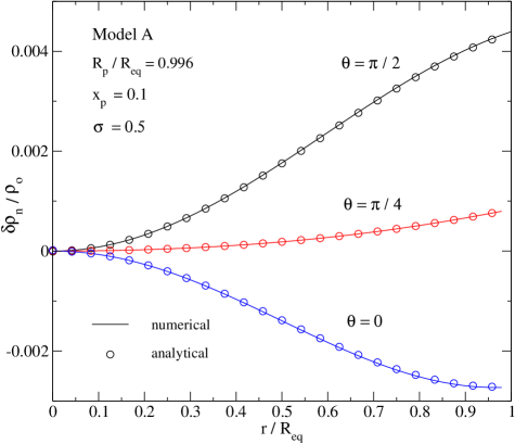
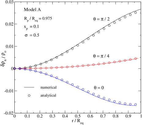
We have tested our code against the analytical solution for the EoS (10) determined by Prix et al. (2002) in the slow-rotation approximation. We select two slowly rotating models with axis ratio $0.996$ and $0.975$, respectively. The models have the same proton fraction and symmetry energy term, i.e. $x_{\mathrm{p}}=0.1$ and $\sigma=0.5$. The non-corotating corrections correspond to a relative angular velocity $\left(\delta\Omega_{\mathrm{n}},\delta\Omega_{\mathrm{p}}\right)=\left(1,0\right)$ with constant central chemical potential, c.f. (28). In Fig. 1, we show the radial profile of the perturbed neutron mass density $\delta\rho_{\mathrm{n}}/\rho_{0}$ for the three angles $\theta=0,\pi/4$ and $\pi/2$, respectively. In the slowest rotating model, the agreement between the numerical and the analytical solutions is evident. In the second model, with axis ratio $0.975$ the two solutions begin to differ, as expected. The slow-rotation solution becomes less accurate as the star’s rotation increases. The same behaviour is found for non-corotating solutions with constant mass, i.e. when $\delta M_{\mathrm{x}}=0$. This comparison gives us confidence in our numerically generated background models.

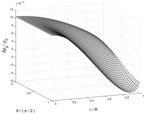
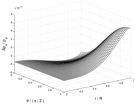
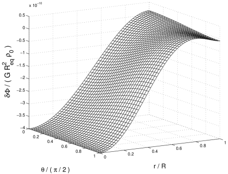
For the sequence of constant mass models, we show in Figs. 2 and 3 the non-corotating mass density pertubations $\delta\rho_{\mathrm{x}}/\rho_{0}$ and the gravitational potential perturbation $\delta\Phi$ for the C2 model. These are solutions to equations (25)–(26) with $\delta\Omega_{\mathrm{p}}=-10^{-6}$ and $\delta\Omega_{\mathrm{n}}=7.74\times 10^{-8}$, which were used as initial conditions for the glitch simulations discussed by Sidery et al. (2010).

Figure 3: We show, for the C2 model and the non-corotating configuration from Fig. 2, the result for the dimensionless gravitational potential $\delta\Phi/\left(GR_{eq}^{2}\rho_{0}\right)$.

4 Perturbation Equations

The dynamics of a superfluid neutron star can be studied by linearizing the system of differential equations (1)–(3). In the inertial frame, the Eulerian perturbation equations are given by

$$\partial_{t}\left(\delta\mathbf{v}_{\mathrm{x}}+\varepsilon_{\mathrm{x}}\delta\mathbf{w}_{\mathrm{y}\mathrm{x}}\right)+\Omega\,\partial_{\phi}\delta\mathbf{v}_{\mathrm{x}} = -\nabla\delta\tilde{\mu}_{\mathrm{x}}-\nabla\delta\Phi-2\mathbf{\Omega}\times\delta\mathbf{v}_{\mathrm{x}}+\frac{\delta\mathbf{f^{\mathrm{x}}}}{\rho_{\mathrm{x}}}\,,$$ (32)

$$\left(\partial_{t}+\Omega\,\partial_{\phi}\right)\,\delta\rho_{\mathrm{x}} = -\nabla\cdot\left(\rho_{\mathrm{x}}\delta\mathbf{v}_{\mathrm{x}}\right)\,,$$ (33)

$$\nabla^{2}\delta\Phi = 4\pi G\,\delta\rho\,,$$ (34)

where $\phi$ is the azimuthal angle associated with the rotational motion, and the perturbed mutual friction force is (in the case of a co-rotating background)

$$\delta\mathbf{f}^{\mathrm{x}}=2\rho_{\mathrm{n}}\mathcal{B}^{\prime}\mathbf{\Omega}\times\delta\mathbf{w}_{\mathrm{x}\mathrm{y}}+2\rho_{\mathrm{n}}\mathcal{B}\,\hat{\mathbf{\Omega}}\times\mathbf{\Omega}\times\delta\mathbf{w}_{\mathrm{x}\mathrm{y}}\,.$$ (35)

The chemical potential perturbations can be expressed in terms of the mass density perturbations using equation (27).

In order to solve numerically equations (32)–(33) we use the conjugate momentum perturbations $\delta\mathbf{p}_{\mathrm{x}}$ as dynamical variables. These are given by

$$\delta\mathbf{p}_{\mathrm{n}} = \left(1-\varepsilon_{\mathrm{n}}\right)\delta\mathbf{v}_{\mathrm{n}}+\varepsilon_{\mathrm{n}}\delta\mathbf{v}_{\mathrm{p}}\,,$$ (36)

$$\delta\mathbf{p}_{\mathrm{p}} = \varepsilon_{\mathrm{p}}\delta\mathbf{v}_{\mathrm{n}}+\left(1-\varepsilon_{\mathrm{p}}\right)\delta\mathbf{v}_{\mathrm{p}}\,,$$ (37)

where we recall that $\rho_{\mathrm{p}}\varepsilon_{\mathrm{p}}=\rho_{\mathrm{n}}\varepsilon_{\mathrm{p}}$. By inverting these relations we can determine the velocity fields at any time step,

$$\delta\mathbf{v}_{\mathrm{n}} = \frac{\left(1-\varepsilon_{\mathrm{p}}\right)\delta\mathbf{p}_{\mathrm{n}}-\varepsilon_{\mathrm{n}}\delta\mathbf{p}_{\mathrm{p}}}{1-\bar{\varepsilon}}\,,$$ (38)

$$\delta\mathbf{v}_{\mathrm{p}} = \frac{-\varepsilon_{\mathrm{p}}\delta\mathbf{p}_{\mathrm{n}}+\left(1-\varepsilon_{\mathrm{n}}\right)\delta\mathbf{p}_{\mathrm{p}}}{1-\bar{\varepsilon}}\,,$$ (39)

where $\bar{\varepsilon}\equiv\varepsilon_{\mathrm{n}}+\varepsilon_{\mathrm{p}}=\varepsilon_{\mathrm{n}}/x_{\mathrm{p}}$.

The time evolution of the non-axisymmetric perturbation equations is a three-dimensional problem in space. However, linear perturbations on an axisymmetric background can be expanded in terms of a set of basis functions $\left(\cos m\phi\,,\sin m\phi\right)$, where $m$ is the azimuthal harmonic index (Papaloizou & Pringle, 1980). The mass density perturbations as well as the other perturbation quantities then take the following form (Jones et al., 2002; Passamonti et al., 2009a)

$$\delta\rho\left(t,r,\theta,\phi\right)=\sum_{m=0}^{m=\infty}\left[\delta\rho_{m}^{+}\left(t,r,\theta\right)\cos m\phi+\delta\rho_{m}^{-}\left(t,r,\theta\right)\sin m\phi\right]\,.$$ (40)

With this Fourier expansion the perturbation equations decouple with respect to $m$ and the problem becomes two-dimensional. In particular, for the axisymmetric case ($m=0$) only the $\delta\rho_{0}^{+}$ component survives.

4.1 Boundary Conditions

In this work, we study axisymmetric ($m=0$) and non-axisymmetric oscillations ($m=2$) of a superfluid neutron star with equatorial and rotational axis symmetry. The numerical domain extends over the region $0\leq r/R(\theta)\leq 1$ and $0\leq\theta\leq\pi/2$, and we need to impose boundary conditions at the surface, origin, rotational axis and equator.

We first discuss the boundary conditions at the origin ($r=0$) and the rotational axis ($\theta=0$), where the perturbation equations must be regular. Let us denote by $\delta\psi$ a general scalar perturbation, such as the mass density $\delta\rho_{\mathrm{x}}$, the chemical potential $\delta\tilde{\mu}_{\mathrm{x}}$ and the gravitational potential $\delta\Phi$. For axi-symmetric and non-axisymmetric oscillations, we have to impose the following conditions, respectively :

$$\left.\frac{\partial\delta\psi}{\partial r}\right|_{r=0} = \left.\frac{\partial\delta\psi}{\partial\theta}\right|_{\theta=0}=0\quad\mbox{for}\quad m=0\,,$$ (41)

$$\left.\delta\psi\right|_{r=0} = \hskip 7.96677pt\left.\delta\psi\right|_{\theta=0}=0\quad\mbox{for}\quad m=2\,.$$ (42)

For the velocity fields $\delta\mathbf{v}_{\mathrm{x}}$, we impose that there must be no mass flux across the origin ($r=0$) for both axisymmetric and non-axisymmetric perturbations:

$$\left.\delta v^{r}_{\mathrm{x}}\right|_{r=0}=0\,.$$ (43)

At the rotational axis ($\theta=0$), we impose the following conditions:

$$\frac{\partial\delta v^{r}_{\mathrm{x}}}{\partial\theta} = \delta v^{\theta}_{\mathrm{x}}=\delta v^{\phi}_{\mathrm{x}}=0\quad\mbox{for}\quad m=0\,,$$ (44)

$$\delta v^{r}_{\mathrm{x}} = \delta v^{\theta}_{\mathrm{x}}=\delta v^{\phi}_{\mathrm{x}}=0\quad\mbox{for}\quad m=2\,.$$ (45)

At the equator ($\theta=\pi/2$), the reflection symmetry divides the perturbations into two sets with opposite parity (Passamonti et al., 2009b). In the Type I parity class, the scalar perturbations $\delta\psi$ and the velocity satisfy the following conditions:

$$\frac{\partial\delta\psi}{\partial\theta}=\frac{\partial\delta v^{r}_{\mathrm{x}}}{\partial\theta}=\delta v^{\theta}_{\mathrm{x}}=\frac{\partial\delta v^{\phi}_{\mathrm{x}}}{\partial\theta}=0\,.$$ (46)

Meanwhile, the Type II class is such that:

$$\delta\psi=\delta v^{r}_{\mathrm{x}}=\frac{\partial\delta v^{\theta}_{\mathrm{x}}}{\partial\theta}=\delta v^{\phi}_{\mathrm{x}}=0\,.$$ (47)

The outer layers of a mature neutron star form an elastic crust made up of nuclei. The crust is an important aspect that is yet to be implemented in our numerical model (although we are making progress on it). Our current model is simplified, in the sense that we assume that superfluid neutrons and protons are present throughout the stellar volume. We then impose the standard boundary condition of a free surface, i.e. require that the Lagrangian perturbation of the individual chemical potentials vanish at the surface, i.e.

$$\Delta\tilde{\mu}_{\mathrm{x}}=\delta\tilde{\mu}_{\mathrm{x}}+\mathbf{\xi}_{\mathrm{x}}\cdot\nabla\tilde{\mu}_{\mathrm{c}}=0\,.$$ (48)

The vector field $\mathbf{\xi}_{\mathrm{x}}$ is the Lagrangian displacement of the x-fluid component (Andersson, Comer & Grosart, 2004). The value of the perturbed chemical potential $\delta\tilde{\mu}_{\mathrm{x}}$ at the surface is determined from equation (48) at each time step.

5 Gravitational-wave Extraction

In order to study the gravitational-wave signal emitted by pulsating superfluid neutron stars, we have implemented the quadrupole formula for both axisymmetric and non-axisymmetric oscillations. We will now discuss this implementation, in particular, the momentum and stress formula that we use to improve the numerical gravitational-wave extraction.

The gravitational-wave strain can be determined using the quadrupole formula (Thorne, 1980):

$$h_{ij}^{2m}=\frac{G}{c^{4}}\frac{1}{r}\sum_{m=-l}^{l}\frac{d^{2}\mathcal{I}}{dt^{2}}^{2m}\,T_{ij}^{E2,2m}\,,$$ (49)

where $T_{ij}^{E2,2m}$ is the pure spin tensor harmonic which has “electric-type” parity, i.e. $\left(-1\right)^{l}$ (Thorne, 1980). In this work, we focus only on the $m=0$ and $m=2$ pulsations. In the orthonormal basis of spherical coordinates, the components of the $(l,m)=(2,0)$ and $(l,m)=(2,2)$ spin tensor harmonics are, respectively, given by

$$T_{\theta\theta}^{E2,20} = \frac{1}{8}\sqrt{\frac{15}{\pi}}\sin^{2}\theta\,,$$ (50)

and

$$T_{\theta\theta}^{E2,22} = T_{\phi\phi}^{E2,22}=\frac{1}{16}\sqrt{\frac{10}{\pi}}\left(1+\cos^{2}\theta\right)e^{2i\phi}\,,$$ (51)

$$T_{\theta\phi}^{E2,22} = \frac{i}{16}\sqrt{\frac{10}{\pi}}\cos\theta\,e^{2i\phi}\,.$$ (52)

The quantity $\mathcal{I}^{2m}$ is the quadrupole moment, in the case of a two-fluid star defined by;

$$\mathcal{I}^{2m}=\frac{16\pi}{15}\sqrt{3}\int d\mathbf{r}\,\delta\rho\,r^{2}\,Y_{2m}^{\ast}=\frac{16\pi}{15}\sqrt{3}\int d\mathbf{r}\,\left(\delta\rho_{\mathrm{n}}+\delta\rho_{\mathrm{p}}\right)r^{2}\,Y_{2m}^{\ast}\,,\\$$ (53)

where the spherical harmonics $Y_{2m}$ for the $m=0$ and $m=2$ cases are given by

$$Y_{20} = \frac{1}{4}\sqrt{\frac{5}{\pi}}\left(3\cos^{2}\theta-1\right)=\frac{1}{2}\sqrt{\frac{5}{\pi}}P_{20}\left(\cos\theta\right)\,,$$ (54)

$$Y_{22} = \frac{1}{4}\sqrt{\frac{15}{2\pi}}\sin^{2}\theta\,e^{2i\phi}\,.$$ (55)

where $P_{20}\left(\cos\theta\right)$ is the Legendre polynomial.

It is well-known that, the numerical calculation of the second order time derivative of the quadrupole moment in equation (49) could lead to inaccurate results (Finn & Evans, 1990). However, the accuracy of the gravitational-wave extraction can be improved by transforming equation (49) into either the perturbed momentum formula, with a first order time derivative, or the perturbed stress formula, where the time derivatives are absent (Finn & Evans, 1990). In this work, we use both these prescriptions in order to check the wave extraction accuracy.

For axisymmetric oscillations, $m=0$, the gravitational strain can be written as follows:

$$h^{20}=\frac{G}{c^{4}}\frac{\sin^{2}\theta}{r}\sum_{\mathrm{x}}A_{\mathrm{x}}^{20}\,,$$ (56)

where the quantity $A_{\mathrm{x}}^{20}$ is defined by

$$A^{20}_{\mathrm{x}}\equiv\frac{d^{2}}{dt^{2}}\int d\mathbf{r}\,\delta\rho_{\mathrm{x}}\,r^{2}\,P^{20}\,.$$ (57)

We can reduce the order of the time derivative by using the method developed by Finn & Evans (1990), and obtain the perturbed momentum formula:

$$A^{20}_{\mathrm{x}}\equiv 2\frac{d}{dt}\int d\mathbf{r}\,r\rho_{\mathrm{x}}\left(\delta v_{\mathrm{x}}^{r}\,P^{20}+\frac{\delta v_{\mathrm{x}}^{\theta}}{2}\frac{\partial P}{\partial\theta}^{20}\right)\,,$$ (58)

and the perturbed stress formula:

$$A^{20}_{\mathrm{x}} \equiv 2\int d\mathbf{r}\left\{-\Omega r\sin\theta\,\rho_{\mathrm{x}}\,\delta v_{\mathrm{x}}^{\phi}-\frac{1}{2}\left(\Omega r\sin\theta\right)^{2}\delta\rho_{\mathrm{x}}\right.$$ (59)

$$+ \left.\frac{1}{4\pi}\left[\nabla_{r}\Phi\nabla_{r}\delta\Phi P^{20}\left(\cos\theta\right)+\nabla_{\theta}\Phi\nabla_{\theta}\delta\Phi\,P^{20}\left(\sin\theta\right)+\frac{1}{2}\left(\nabla_{r}\Phi\nabla_{\theta}\delta\Phi+\nabla_{\theta}\Phi\nabla_{r}\delta\Phi\right)\partial_{\theta}P^{20}\left(\cos\theta\right)\right]\right\}\,,$$

where the gradient components $\nabla_{i}$ in eqaution (59) are determined in the orthonormal spherical basis, i.e. $\nabla=\left(\partial_{r},\frac{1}{r}\partial_{\theta},\frac{1}{r\sin\theta}\partial_{\phi}\right)$. At the end of the day, the quantity $A^{20}_{\mathrm{x}}$ in the strain equation (56) can be determined from either of the three equations (57)–(59).

Figure 4: We compare the gravitational-wave extraction results for axisymmetric and non-axisymmetric oscillations. The signal is generated by perturbing the stellar model C2, and the illustrated quantities are dimensionless. The left panel shows the dimensionless code quantity $A^{20}_{\ast}$ determined from three equivalent equations, respectively, the second time derivative of the quadrupole moment (dot-dashed line), the momentum-formula (solid-line) and the stress formula (dashed-line). In the right panel, we show the waveform of the $m=2$ non-axisymmetric oscillations for the perturbed C2 model. The upper and lower right panels displays respectively the real part $A^{22}_{R}$ and the imaginary part $A^{22}_{I}$ of the dimensionless quantity $A^{22}_{\ast}$ determined by the code. We compare the signal extraction to the momentum-formula (solid-line) and the stress formula (dashed-line).

For non-axisymmetric oscillations with $l=m=2$, the two independent polarizations of the strain can be written as follows:

$$h_{\theta\theta}^{22}-ih_{\theta\phi}^{22}=h^{22}{}_{-2}Y^{22}\,,$$ (60)

where ${}_{-2}Y^{22}$ is the $s=-2$ spin-weighted spherical harmonics,

$${}_{-2}Y^{22}=\frac{1}{8}\sqrt{\frac{5}{\pi}}\left(1+\cos\theta\right)^{2}e^{2i\phi}\,,$$ (61)

and we have defined the quantity

$$h^{22}\equiv\frac{G}{c^{4}}\frac{8\pi}{15}\frac{\sqrt{3}}{r}\frac{d^{2}}{dt^{2}}\int d\mathbf{r}\,\delta\rho\,r^{2}Y_{22}^{\ast}\,.$$ (62)

We can then re-write equation (62) as follows:

$$h^{22}=\frac{G}{c^{4}}\frac{8\pi}{15}\frac{\sqrt{3}}{r}\sum_{\mathrm{x}}A_{\mathrm{x}}^{22}\,,$$ (63)

where

$$A^{22}_{\mathrm{x}}\equiv\frac{d^{2}}{dt^{2}}\int d\mathbf{r}\,\delta\rho_{\mathrm{x}}\,r^{2}Y_{22}^{\ast}\,.$$ (64)

In equation (64), the order of the time derivatives can be reduced by using the equations of motion (see Appendix A for more details). This leads to the following expression:

$$A^{22}_{\mathrm{x}}\equiv 2\frac{d}{dt}\int d\mathbf{r}\left\{\rho_{\mathrm{x}}r\left[\left(\delta v^{r}_{\mathrm{x}}-i\frac{\delta v^{\phi}_{\mathrm{x}}}{\sin\theta}\right)Y_{22}^{\ast}+\frac{\delta v_{\mathrm{x}}^{\theta}}{2}Y_{22,\theta}^{\ast}\right]-i\Omega r^{2}\delta\rho_{\mathrm{x}}\,Y_{22}^{\ast}\right\}\,.$$ (65)

For linear perturbations on a corotating background, we can further transform equation (65) into the following expression:

$$A^{22}_{\mathrm{x}} \equiv \frac{1}{2}\sqrt{\frac{15}{2\pi}}\int d\mathbf{r}\left\{-2\rho_{\mathrm{x}}\Omega r\sin\theta\left[\delta v^{\phi}_{\mathrm{x}}+i\left(\sin\theta\delta v^{r}_{\mathrm{x}}+\cos\theta\delta v^{\theta}_{x}\right)\right]-\left(\Omega r\sin\theta\right)^{2}\delta\rho_{\mathrm{x}}\right.$$ (66)

$$+ \left.\frac{1}{4\pi}\left[\sin^{2}\theta\,\nabla_{r}\Phi\nabla_{r}\delta\Phi+\cos^{2}\theta\,\nabla_{\theta}\Phi\nabla_{\theta}\delta\Phi+\sin\theta\cos\theta\left(\nabla_{r}\Phi\nabla_{\theta}\delta\Phi+\nabla_{\theta}\Phi\nabla_{r}\delta\Phi\right)\right.\right.$$

$$- \left.\left.i\left(\sin\theta\nabla_{r}\Phi+\cos\theta\nabla_{\theta}\Phi\right)\nabla_{\phi}\delta\Phi\right]\right\}\,,$$

where the time derivatives are absent. In equations (65) and (66), the perturbations are determined in the inertial frame.

The energy radiated as gravitational waves is determined by the following equation (Thorne, 1980):

$$E_{rad}^{2m}=\frac{1}{32\pi}\frac{G}{c^{5}}\int_{-\infty}^{\infty}\left|\frac{d^{3}\mathcal{I}}{dt^{3}}^{2m}\right|^{2}dt\,.$$ (67)

By using Parseval’s Theorem we can write equation (67) for the $(2,0)$ and $(2,2)$ components as follows:

$$E_{rad}^{20} = \int_{0}^{\infty}\frac{dE}{d\nu}^{20}d\nu=\frac{16}{15}\pi^{2}\frac{G}{c^{5}}\int_{0}^{\infty}\nu^{2}\left|\hat{A}^{20}\right|^{2}d\nu\,,$$ (68)

$$E_{rad}^{22} = \int_{0}^{\infty}\frac{dE}{d\nu}^{22}d\nu=\frac{64}{75}\pi^{3}\frac{G}{c^{5}}\int_{0}^{\infty}\nu^{2}\left|\hat{A}^{22}\right|^{2}d\nu\,,$$ (69)

where $A^{2m}=A^{2m}_{\mathrm{n}}+A^{2m}_{\mathrm{p}}$, and $\hat{A}^{2m}$ is its Fourier transformation.

The characteristic strain of the gravitational-wave signal is then given by (Flanagan & Hughes, 1998):

$$h_{c}\left(\nu\right)\equiv\sqrt{\frac{{2G}}{\pi^{2}c^{3}}}\frac{1}{d}\sqrt{\frac{dE}{d\nu}}\,,$$ (70)

where $d$ is the source distance. The strains $h^{20}$ and $h^{22}$ are related to the dimensionless quantities $A_{\ast}^{20}$ and $A_{\ast}^{22}$ used in the numerical code by the following expressions:

$$h^{20} = 1.414\times 10^{-17}A_{\ast}^{20}\left(M^{\ast}\right)^{-2}\left(\frac{M}{1.4M_{\odot}}\right)^{2}\left(\frac{R_{eq}}{10\,\rm{km}}\right)^{-1}\left(\frac{1\ \rm{kpc}}{d}\right)\sin^{2}\theta\,,$$ (71)

$$h^{22} = 4.109\times 10^{-17}A_{\ast}^{22}\left(M^{\ast}\right)^{-2}\left(\frac{M}{1.4M_{\odot}}\right)^{2}\left(\frac{R_{eq}}{10\,\rm{km}}\right)^{-1}\left(\frac{1\ \rm{kpc}}{d}\right)\,.$$ (72)

Similar relations provide the characteristic strain

$$h_{c}^{20} = 1.513\times 10^{-18}|\hat{A}^{20}_{\ast}|\left(M^{\ast}\right)^{-3/2}\left(\frac{M}{1.4M_{\odot}}\right)^{3/2}\left(\frac{R_{eq}}{10\,\rm{km}}\right)^{1/2}\left(\frac{1\ \rm{kpc}}{d}\right)\left(\frac{\nu}{1\rm{kHz}}\right)\,,$$ (73)

$$h_{c}^{22} = 2.398\times 10^{-18}|\hat{A}^{22}_{\ast}|\left(M^{\ast}\right)^{-3/2}\left(\frac{M}{1.4M_{\odot}}\right)^{3/2}\left(\frac{R_{eq}}{10\,\rm{km}}\right)^{1/2}\left(\frac{1\ \rm{kpc}}{d}\right)\left(\frac{\nu}{1\rm{kHz}}\right)\,.$$ (74)

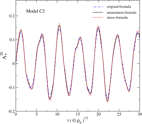
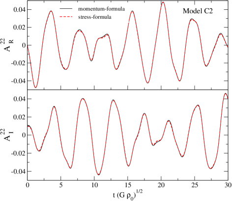
As a first test of the numerical implementation, we compare the gravitational-wave extraction formulae for the axisymmetric and non-axisymmetric oscillations. We evolve the C2 model with a density perturbation and extract the signal using equations (57)–(59) for the $m=0$ pulsations, and (65)–(66) for the $m=2$ oscillations. Typical results are shown in Figure 4. We generally find good agreement between the different numerical results, although we note that (as expected) the momentum and stress formulae produce a smoother signal than the “raw” quadrupole formula (57).

As an additional test, we have used the relativistic numerical code developed by Nagar & Diaz (2004) and Passamonti et al. (2007) to test the results of the gravitational-wave extraction routine. In the relativistic case, the linear perturbations of non-rotating relativistic stars were evolved and the signal was extracted using the Zerilli function (Zerilli, 1970). From the Newtonian approach used in the current work, it is evident that we cannot accurately reproduce the relativistic results. However, we can establish that our calculations provide a good estimate of the amplitude of the gravitational-wave strain. To this end, we consider a star with mass $M=1.4M_{\odot}$ and radius $R=14~{}\rm{km}$, and evolve the relativistic code with an initial enthalpy perturbation, which produces an averaged pulsational kinetic energy of $\langle E_{k}\rangle\simeq 5.62\times 10^{-9}M_{\odot}c^{2}$, where $c$ is the speed of ligth. The related gravitational-wave strain is almost monochromatic and for a source at $10\,\rm{kpc}$ the maximal amplitude is $\left.h^{20}\right|_{max}\simeq 2.18\times 10^{-22}\sin^{2}\theta$.

Table 2: Comparison of the first three $l=0,2$ ordinary and superfluid mode frequencies and the Prix & Rieutord (2002) results. The star is the non-rotating C0 model, which corresponds to model III of Prix & Rieutord (2002), where the entrainment parameter $\bar{\varepsilon}$ is zero. Frequencies are given in units of $\sigma/\sqrt{G\rho_{0}}$ and have been determined with an FFT of the gravitational strain time evolution. For this specific numerical simulation the frequency error bar is $\Delta\sigma/\sqrt{G\rho_{0}}=5.58\times 10^{-3}$. The Prix and Rieutord values are denoted by PR. In the final column we show the relative error between our and PR results.

Mode	$\sigma/\sqrt{G\rho_{0}}$	$\sigma/\sqrt{G\rho_{0}}$	$\Delta\sigma/\sigma$
	PR		[ % ]
$\rm{F}^{\mathrm{o}}$	1.91361	1.92743	0.7
$\rm{F}^{\mathrm{s}}$	2.52823	2.53376	0.2
$\rm{H}_{1}^{\mathrm{o}}$	3.94917	3.94911	$<$ 0.1
$\rm{H}_{1}^{\mathrm{s}}$	4.20552	4.20420	$<$ 0.1
$\rm{H}_{2}^{\mathrm{o}}$	5.61069	5.52870	1.5
$\rm{H}_{2}^{\mathrm{s}}$	5.93799	5.92165	0.3
$\rm{f}^{~{}\mathrm{o}}$	1.33511	1.33178	0.2
$\rm{f}^{~{}\mathrm{s}}$	1.83142	1.82281	0.5
$\rm{p}_{1}^{\mathrm{o}}$	3.47686	3.48786	0.3
$\rm{p}_{1}^{\mathrm{s}}$	3.68465	3.69878	0.4
$\rm{p}_{2}^{\mathrm{o}}$	5.24187	5.25802	0.3
$\rm{p}_{2}^{\mathrm{s}}$	5.51946	5.52876	0.2

With our 2D Newtonian code, we then evolve in time non-radial oscillations of a superfluid non-rotating star for both the EoS (10) and (11). The kinetic energy of oscillating superfluid stars can be determined by the following expression:

$$E_{k}=\frac{1}{2}\int d\mathbf{r}\left[\rho_{\mathrm{n}}\left(1-\varepsilon_{\mathrm{n}}\right)|\delta\mathbf{v}_{\mathrm{n}}|^{2}+2\rho_{\mathrm{n}}\varepsilon_{\mathrm{n}}\delta\mathbf{v}_{\mathrm{n}}\cdot\delta\mathbf{v}_{\mathrm{p}}+\rho_{\mathrm{p}}\left(1-\varepsilon_{\mathrm{p}}\right)|\delta\mathbf{v}_{\mathrm{p}}|^{2}\right]\,.$$ (75)

If we evolve oscillations that have the same pulsational kinetic energy as in the case studied with the relativistic code, we obtain $\left.h^{20}\right|_{max}\simeq 1.55\times 10^{-22}\sin^{2}\theta$ for model A0 and $\left.h^{20}\right|_{max}\simeq 1.433\times 10^{-22}\sin^{2}\theta$ for model C0. In this calculation, we have used equation (71) with the parameters of the relativistic stellar model. This test shows that we can be confident that the implementation of the quadruple formula in our code provides reasonable results, in accordance with the expected relation between the pulsational kinetic energy and the gravitational-wave strain.

6 Results

Having formulated the time-evolution problem and described our implementation of the gravitational-wave extraction, we will now discuss our results. In this section, we focus on the effects of the gravitational potential perturbation and the mutual friction force on axisymmetric and non-axisymmetric oscillations. We also provide a more detailed analysis of the gravitational-wave signal generated by the basic glitch model that we discussed in a previous work (Sidery et al., 2010).

The pulsation dynamics is studied with a numerical code that evolves in time the system of hyperbolic perturbation equations (32)–(33), solving at each time step the perturbed Poisson equation (34). The part of the code that evolves the hyperbolic equations uses the same technology as in previous work (Passamonti et al., 2009a, b), whereas the elliptic equation (34) is solved using a pseudo spectral method. The numerical grid is two-dimensional and covers the volume of the star, i.e. the region $0\leq r\leq R(\theta)$ and $0\leq\theta<\pi/2$. The implementation uses a new radial coordinate $x=x(r,\theta)$, which is fitted to surfaces of constant chemical potential. This allows us to consider stars that are highly deformed by rotation. The perturbation variables are discretized on this grid and updated in time with a Mac-Cormack algorithm. The numerical simulations are stabilised from high frequency noise with the implementation of a fourth order Kreiss-Oliger numerical dissipation. More technical details have been discussed in Passamonti et al. (2009a, b).

Figure 5: This figure displays the effect of rotation on the quasi-radial and axisymmetric quadrupole modes. We use the sequence of models A, with entrainment parameter $\bar{\varepsilon}=0.5$, proton fraction $x_{\mathrm{p}}=0.1$ and vanishing symmetry energy term. On the horizontal axis the angular velocity is rescaled with the Kepler angular velocity $\Omega_{K}$, while the mode frequencies are given in dimensionless units and for a rotating frame. In the left panel, we show some “ordinary modes”, which are due to the co-moving degrees of freedom. We identify the $l=0$ and $l=2$ fundamental modes and the first three quasi-radial overtones and $l=2$ pressure modes. In the right panel, we show instead the “superfluid modes”, which correspond to the counter-moving degrees of freedom. In this case we show the modes up to the second overtones. For these non-stratified models, the ordinary and superfluid modes are decoupled.

In order to solve the elliptic equation (34) with a spectral method, and save computational time, we set up a second numerical grid with lower resolution. This is important, since the spectral solver must be used at each time step, leading to a significant slow-down of the simulations. However, the lower resolution on the spectral grid does not affect the results, as spectral elliptic solvers provide highly accurate and rapidly convergent solutions already for relatively coarse grids (Grandclément & Novak, 2009). Therefore, at each time step we first fit the mass density perturbation $\delta\rho$ on the spectral grid and then use the spectral routines to determine the gravitational potential perturbation $\delta\Phi$. Subsequently, we fit the new value of $\delta\Phi$ to the original grid for the hyperbolic equations and carry on the evolution. The numerical code provides stable simulations for all rotating stellar models considered in this paper.

In this work, our choice of variables differs from that of Passamonti et al. (2009a). We evolve the velocity perturbations of the two-fluids components instead of the “mass flux” perturbations of the co-moving and counter-moving degrees of freedom. The two formulations are obviously mathematically equivalent, but we wanted to develop a code based on the new set of variables in order to explore which formulation is best suited for future extensions. This is important, as we plan to add more realistic physics to our models by implementing an elastic crust region. As a first test, we compare the results of the new code to those obtained in Cowling approximation by Passamonti et al. (2009a). Neglecting the perturbation of the gravitational potential, i.e. setting $\delta\Phi=0$, we find a complete agreement between the two numerical codes.

In order to study the spectral properties discussed below, in Sec. 6.1 and 6.2, we consider “generic” initial conditions that excite a large set of oscillation modes. For Type I perturbations we provide the following expression for the mass density:

$$\delta\rho_{\mathrm{n}}=-\delta\rho_{\mathrm{p}}=\left(\frac{r}{R\left(\theta\right)}\right)^{l}Y_{ll}\left(\theta,\phi\right)\,,$$ (76)

where neutrons and protons are initially counter-moving. For Type II perturbations, we excite mainly normal and superfluid r-modes with the following initial data:

$$\delta\mathbf{v}_{\mathrm{n}}=-\delta\mathbf{v}_{\mathrm{p}}=\left(\frac{r}{R\left(\theta\right)}\right)^{l}Y_{ll}^{B}\left(\theta,\phi\right)\,,$$ (77)

where $Y_{ll}^{B}\left(\theta,\phi\right)$ is a magnetic spherical harmonic (Thorne, 1980). For the glitch simulations, we use the non-corotating solutions derived in Sec. 3.2.

We test the elliptic solvers by comparing the mode frequencies extracted from our time evolutions to those obtained in the frequency domain by Prix & Rieutord (2002). We determine the oscillation frequencies of the non-rotating model C0 (see Table 1), which corresponds to model III of Prix & Rieutord (2002). For the zero entrainment case, i.e. when $(\bar{\varepsilon}=0)$, the results in Table 2 show that the frequencies determined with our code (by an FFT of the time-evolved perturbations) agree very well with those calculated by Prix & Rieutord (2002).

Figure 6: In this figure, we show the axisymmetric modes for the sequence of C models determined in a rotating frame. These stellar models are stratified and the ordinary and superfluid degrees of freedom are coupled. We identify some of the acoustic modes and their dependence on the rotational rate $\Omega/\Omega_{K}$.

6.1 Spectrum

The oscillation spectrum of superfluid rotating neutron stars contains the imprints of two-fluid dynamics and of the mutual friction force. For a single fluid star, the general mode classification is based on the main restoring force that acts on the displaced fluid elements (Cowling, 1941). For nonrotating models without magnetic field and crust, the spectrum is formed by the acoustic, the fundamental and the gravity modes. The acoustic modes are mainly restored by pressure variations and cover the high frequency range of the spectrum, above 1 kHz. At lower frequencies, typically below 100 Hz, composition and thermal gradients generate the class of gravity modes that are restored by buoyancy. The fundamental mode, whose frequency scales with the average stellar density, separates these two classes of modes. In rotating stars, the Coriolis force provides an additional restoring force, leading to the presence of inertial modes. Since the frequency of these modes scales with the rotation rate, they typically lie in the same low frequency region as the g-modes. For rotating stars with composition gradients, the inertial and gravity modes form a unique class with mixed properties, referred to as gravity-inertial modes (for a recent analysis see Passamonti et al., 2009b; Gaertig & Kokkotas, 2009).

In addition to this general classification, any oscillation mode can be labeled by the indices $(l,m)$ associated with the spherical harmonics $Y_{l}^{m}(\theta,\phi)$. In spherical stars, this is due to the decomposition of the perturbation functions in vector harmonics. For rotating stars, we can use the same description as long as we can track a mode back to its non-rotating limit. Finally, for any value of $(l,m)$, the oscillation modes can be ordered by the number of radial nodes in their eigenfunctions. The fundamental mode ${}^{l}\textrm{f}$ does not have radial nodes, while the series of pressure ${}^{l}\textrm{p}_{i}$ and gravity modes ${}^{l}\textrm{g}_{i}$ have $i$ nodes.

In superfluid neutron stars, the additional degree of freedom enriches the dynamics. The two fluids can oscillate both in phase and counter-phase. The co-moving degree of freedom produces the class of “ordinary modes”, very similar to the single fluid results described above. There is, however, one important difference: the gravity modes are absent in superfluid stars (Lee, 1995; Andersson & Comer, 2001; Prix & Rieutord, 2002). The counter-moving degree of freedom generates a new class of acoustic and inertial modes, known as “superfluid” modes. These modes strongly depend on the superfluid aspects, such as entrainment and mutual friction. We will label ordinary and superfluid modes by an upper index, for instance the $l=2$ fundamental ordinary mode will be expressed as ${}^{2}\textrm{f}^{\hskip 1.70717pt\rm{o}}$, while ${}^{2}\textrm{f}^{\hskip 1.70717pt\rm{s}}$ represents the corresponding superfluid mode.

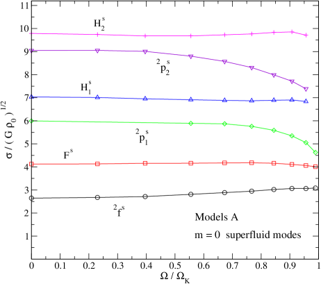
We focus our attention on the quasi-radial ($l=0$) and quadrupole ($l=2$) oscillation modes and study their behaviour in rapidly rotating models all the way to the mass shedding limit. In non-rotating models, the $l=0$ modes are purely radial and do not generate gravitational radiation. However, due to coupling of the different multipoles, this is no longer true in the rotating case. The quasi-radial fundamental mode will be denoted by F and its $i$ overtones by $\textrm{H}_{i}$. The quadrupole modes ($l=2$) are expected to be dominant in the gravitational signal, and we study both axisymmetric and non-axisymmetric oscillations. These correspond to $m=0$ and $m=2$ respectively.

We start by considering the axisymmetric oscillations for the two sequences of rotating models A and C. For a small velocity lag between the two fluids, the entrainment parameter $\bar{\varepsilon}$ can be chosen independently from the background model (see Section 2.1). Recent work suggests that it can assume values in the range $0.2\leq\bar{\varepsilon}\leq 0.8$ (Chamel, 2008). Here, we consider only the case $\bar{\varepsilon}=0.5$, as the effect of this parameter on the oscillation frequencies has been already discussed elsewhere (Prix & Rieutord, 2002; Passamonti et al., 2009a; Haskell et al., 2009). The parameters $\varepsilon_{\mathrm{x}}$ for the two fluids are then given by $\varepsilon_{\mathrm{n}}=x_{\mathrm{p}}\,\bar{\varepsilon}$ and $\varepsilon_{\mathrm{p}}=\bar{\varepsilon}-\varepsilon_{\mathrm{n}}$. For models A we must also specify the proton fraction and the symmetry energy term. These are, respectively, set to $x_{\mathrm{p}}=0.1$ and $\sigma=0$. For a discussion of the effect of $\sigma$ on the spectrum, see Passamonti et al. (2009a). From the numerical simulations we determine the mode frequencies with an FFT of the time-evolved perturbation variables. In order to identify the different modes, we use also the eigenfunction extraction technique developed by Stergioulas et al. (2004) and Dimmelmeier et al. (2006).

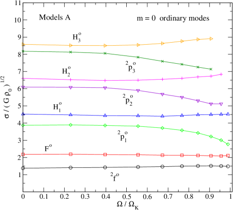
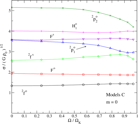
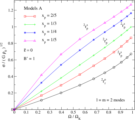
In Fig. 5 we show, for the non-stratified A models, some of the axisymmetric frequencies of the quasi-radial ($l=0$) and quadrupole ($l=2$) modes. In the left and right panels we show the “ordinary” and “superfluid” modes, respectively. These two mode families are decoupled in non-stratified stars, and in fact the results in Fig. 5 do not hint at any interaction in the spectrum. However, within the sets of ordinary and superfluid modes avoiding crossings may appear. For instance, the ordinary quasi-radial mode $\rm{H}_{1}^{\mathrm{o}}$ and the ordinary pressure mode ${}^{2}\rm{p}_{2}^{\mathrm{o}}$ seem to have an avoiding crossing when the star is rotating at $90\%$ of the mass shedding limit. The effects of the chemical coupling on the spectrum is evident in Fig. 6, where we show some of the axisymmetric modes for the C models. In this case, the superfluid fundamental mode ${}^{2}\rm{f}^{\hskip 1.70717pt\mathrm{s}}$ and the ordinary first pressure mode ${}^{2}\rm{p}_{1}^{\mathrm{o}}$ interact through an avoiding crossing near 90% of the Kepler limit.

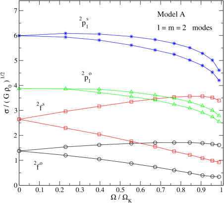
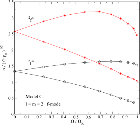
For a given $l$ multipole, the non-axisymmetric modes of non-rotating stars have a degeneracy with respect to $m$. Rotation removes this degeneracy and splits each mode into $2l+1$ distinct branches. Besides the $m=0$ case considered above, we consider the $|m|=2$ modes that have a pro- and retro-grade motion with respect to the star. In Fig. 7, we show the frequencies of the acoustic modes for models A (left panel) and C (right panel). The present results improve on the analysis of Passamonti et al. (2009a), that studied the dependence of the rotational splitting on the entrainment parameter within the Cowling approximation. The main improvement concerns the introduction of the gravitational potential perturbations. However, this does not alter the qualitative effects of rotation on the splitting.

Figure 7: In this figure, we show the rotational splitting of the $l=m=2$ non-axisymmetric modes as measured in the rotating frame. The left and right panels display the modes for the sequence of A and C models respectively.

6.2 Mutual friction effects on the spectrum

In order to study the effects of the mutual friction force on the oscillation spectrum, it is useful to write the momentum equation for the relative motion between protons and neutrons. We can combine the Euler-type equations (32) and obtain the following expression in the rotating frame:

$$\left(1-\bar{\varepsilon}\right)\partial_{t}\delta\mathbf{w}^{\mathrm{p}\mathrm{n}}=-\nabla\left(\delta\tilde{\mu}_{\mathrm{p}}-\delta\tilde{\mu}_{\mathrm{n}}\right)-2\mathcal{\bar{B}}^{\prime}\mathbf{\Omega}\times\delta\mathbf{w}^{\mathrm{p}\mathrm{n}}+2\mathcal{\bar{B}}\,\hat{\mathbf{\Omega}}\times\mathbf{\Omega}\times\delta\mathbf{w}^{\mathrm{p}\mathrm{n}}\ ,$$ (78)

where we have defined

$$\mathcal{\bar{B}}^{\prime}\equiv 1-\frac{\mathcal{B}^{\prime}}{x_{\mathrm{p}}}\,,\qquad\qquad\mathcal{\bar{B}}\equiv\frac{\mathcal{B}}{x_{\mathrm{p}}}\,.$$ (79)

Equation (78) makes the effects of the mutual friction parameters $\mathcal{B}$ and $\mathcal{B}^{\prime}$ more evident. The term that includes $\mathcal{B}$ is dissipative and tends to damp the relative motion, and consequently mainly affects the superfluid modes. If the co- and counter-moving degrees of freedom are coupled, for instance due to the EoS, the mutual friction dissipation affects also the ordinary modes. Results to this effect, have been provided by (Lindblom & Mendell, 1995; Andersson et al., 2009) for the f-modes and (Lindblom & Mendell, 2000; Lee & Yoshida, 2003; Haskell et al., 2009) for the r-modes. The term proportional to $\mathcal{B}^{\prime}$ modifies the Coriolis force, as one can see in equation (78). Its effects are not dissipative, but may change the frequencies of the superfluid modes. This is certainly expected in the case of the inertial modes as they are rotationally restored, but we will see that the non-axisymmetric fundamental modes can also be affected.

The magnitude of the mutual friction can be studied by introducing a dimensionless drag parameter $\mathcal{R}$, defined by (Haskell et al., 2009):

$$\mathcal{B}=\frac{\mathcal{R}}{1+\mathcal{R}^{2}}\,,\qquad\qquad\mathcal{B}^{\prime}=\frac{\mathcal{R}^{2}}{1+\mathcal{R}^{2}}\,.$$ (80)

Two extreme drag regimes can then be discerned for the mutual friction force. In the “weak” drag regime $\mathcal{R}\ll 1$, whereas the “strong” drag regime corresponds to $\mathcal{R}\gg 1$. The most commonly considered cause of mutual friction is the scattering of the electrons off the magnetic field of the neutron vortices. This mechanism is firmly in the weak drag regime, where $\mathcal{B}\ll 1$ and $\mathcal{B}^{\prime}\ll\mathcal{B}$. In this case, we expect the mutual friction to act mainly on the mode damping. It should have negligible effects on the oscillation frequencies themselves.

Figure 8: This figure illustrates the effect, in the weak drag regime, of the mutual friction on the stellar oscillations. For the model C2 with $\bar{\varepsilon}=0.5$, the left panel displays the radial component of the variables $\delta\mathbf{V}_{\mathrm{n}\mathrm{p}}$ (upper panel) and $\delta\mathbf{w}_{\mathrm{n}\mathrm{p}}$ (lower panel) for two long simulations with $\mathcal{B}=0$ and $\mathcal{B}=5\times 10^{-4}$, respectively. The horizontal axis shows the dimensionless evolution time. The lower-left panel shows that the counter-moving degrees of freedom are damped due to mutual friction dissipation. In the right panel, we show an FFT of the function $\delta w_{\mathrm{n}\mathrm{p}}^{r}$ for the $\mathcal{B}=5\times 10^{-4}$ case. In order to study the mode amplitude variation with time, we have performed an FFT of the first part of the simulation, where $0\leq t\left(G\rho_{0}\right)\leq 500$ (solid line), and subsequently of the second part, where $500\leq t\left(G\rho_{0}\right)\leq 1000$ (dashed line). On the horizontal axis is shown the dimensionless mode frequency $\sigma/\left(G\rho_{0}\right)^{1/2}$, as measured in the rotating frame. As expected, the superfluid modes exhibit a faster damping than the ordinary modes.

Recent discussions suggest that the strong drag regime may lead to interesting, potentially important, results (Haskell et al., 2009; Andersson et al., 2009). Since our level of theoretical understanding is not sufficient to rule out this case, we also consider the $\mathcal{R}\gg 1$ regime. From equations (80) we see that in the strong drag regime $\mathcal{B}^{\prime}\simeq 1$ and $\mathcal{B}\ll\mathcal{B}^{\prime}$. The main effect should then be on the mode frequencies, while the dissipation can be considered negligible. In principle, we could explore also the intermediate regime, where $\mathcal{R}\simeq 1$ and both energy dissipation and frequency changes are important. However, this case is essentially a combination of the effects that we can study in the weak and strong regimes. Hence, we do not consider the intermediate regime in this work.

6.2.1 Weak drag regime

Let us first consider the weak drag regime by evolving in time the oscillations of model C2. In Fig. 8 we show the results from two long simulations where we have fixed $\mathcal{R}=0$ and $\mathcal{R}=5\times 10^{-4}$, respectively. In the left panel, we show the grid-averaged value of the velocities $\delta\mathbf{V}_{\mathrm{n}\mathrm{p}}=\delta\mathbf{v}_{\mathrm{n}}+\delta\mathbf{v}_{\mathrm{p}}$ and $\delta\mathbf{w}_{\mathrm{n}\mathrm{p}}$. In the upper-left panel, the two curves appear similar showing a weak damping that is mainly due to the numerical dissipation. In fact, the quantity $\delta\mathbf{V}_{\mathrm{n}\mathrm{p}}$ describes the evolution of the co-moving degree of freedom, which is weakly affected by the weak mutual friction. Looking more carefully at the results, we note that some damping is present in the $\mathcal{R}=5\times 10^{-4}$ case. This is due to the chemical coupling with the counter-moving degree of freedom, which is strongly damped. This is evident from the results in the lower-left panel of Fig. 8, which show that the amplitude of the relative velocity $\delta\mathbf{w}_{\mathrm{n}\mathrm{p}}$ decreases during the evolution.

These results suggest that, as expected, superfluid modes are damped faster than the ordinary modes. In order to study how the mode amplitude changes during the evolution, we divide the time-evolved data into two equal sets and perform an FFT for each part. Results for the variable $\delta\mathbf{w}_{\mathrm{n}\mathrm{p}}$ in the $\mathcal{R}=5\times 10^{-4}$ case are shown in the right panel of Fig. 8. We see that the superfluid fundamental and first pressure modes are damped faster then their ordinary counterparts.

The effect of the mutual friction has also been tested by Sidery et al. (2010), by comparing the glitch spin-up time extracted by our numerical evolutions against an analytical formula derived within a body-averaged approximation.

While our results demonstrate good progress, they are not quite satisfactory in one important respect. Ideally, one would like to be able to extract both oscillation frequency and damping time for the different modes seen in the evolution. However, so far we have not managed to extract the mutual friction damping rate of individual oscillation modes with the desired precision. This is basically because of the fact that the damping is very slow. It is also sensitive to the velocity lag between the two fluid components. At the present time it is not clear to us whether a time-evolution code provides a useful alternative to frequency-domain calculation for the damping-rate problem.

Figure 9: This figure shows the effects of mutual friction, in the strong drag regime, on the rotational splitting of the superfluid $l=m=2$ f-mode. The axis labels are shown in dimensionless units and the mode frequencies are determined in the rotating frame. For the sequence of models A with $\bar{\varepsilon}=0$ and $x_{\mathrm{p}}=1/3$, we study the $\mathcal{B}^{\prime}=0$ and $\mathcal{B}^{\prime}=1$ cases. In the left panel, we show the effects of mutual friction on the pro-grade ${}^{2}\rm{f}^{\mathrm{s}}_{p}$ and retro-grade ${}^{2}\rm{f}_{r}^{\mathrm{s}}$ modes, respectively, and the averaged frequencies $\langle\sigma\rangle=\left(\sigma_{p}+\sigma_{r}\right)/2$ of the two mode patterns. In the right panel, we show the deviation of the $l=m=2$ $\rm{f}^{s}$ mode defined by equation (83). The dashed lines are determined by using equation (84). These empirical relations agree very well with the values of the frequency deviation for the $\mathcal{B}^{\prime}=1$ case, which are shown with filled circles.

6.2.2 Strong drag regime

Next we explore the effects of the mutual friction in the strong drag regime, focussing on the $l=m=2$ superfluid f- and r-modes. The parameter $\mathcal{B}^{\prime}$ now dominates the mutual friction force affecting the Coriolis term in equation (78).

The first aspect we want to understand is whether the rotational splitting of the superfluid f-mode is modified by the $\mathcal{\bar{B}}^{\prime}$ parameter. Based on our expectations, we assume that the frequency of the ${}^{2}\rm{f}^{\mathrm{s}}$ mode is described by the following relation up to order $\Omega^{2}$;

$$\sigma^{\mathrm{s}}=\sigma_{NR}^{s}+c_{1}\left(\bar{\varepsilon},\sigma,\mathcal{\bar{B}}^{\prime},m\right)\Omega+\mathcal{O}\left(\Omega^{2}\right)\,,$$ (81)

where $c_{1}$ depends on the azimuthal index $m$ and the stellar parameters $\bar{\varepsilon},\sigma$ and $\mathcal{\bar{B}}^{\prime}$. For $\mathcal{\bar{B}}^{\prime}=0$, we have already studied the dependence of the ${}^{2}\rm{f}^{\mathrm{s}}$ mode on the entrainment parameter $\bar{\varepsilon}$ and the symmetry energy term $\sigma$ (Passamonti et al., 2009a). Therefore, we focus on the $\bar{\varepsilon}=\sigma=0$ case and vary the parameter $\mathcal{\bar{B}}^{\prime}$. Using our previous results, we can re-write equation (81) as follows:

$$\sigma^{\mathrm{s}}=\sigma_{NR}^{s}+\mathcal{\bar{B}}^{\prime}\Omega+\mathcal{O}\left(\Omega^{2}\right)\,,$$ (82)

We can then test this result against the numerical simulations.

Figure 10: For model A2, we show (in the left panel) how the $l=m=2$ superfluid f-mode depends on the proton fraction in the strong drag regime with $\mathcal{B}^{\prime}=1$. The vertical axis displays the ratio of the quantity $\Delta\sigma$ for the $\mathcal{B}^{\prime}=1$ and $\mathcal{B}^{\prime}=0$ cases, see equation (84). In the right panel, we show the $l=m=2$ ordinary ${}^{2}\rm{r}^{\mathrm{o}}$ and superfluid ${}^{2}\rm{r}^{\mathrm{s}}$ modes for the sequence of models A with $\varepsilon=\sigma=0$ and $\mathcal{R}=10^{3}$ ($\mathcal{B}^{\prime}=1$). In the strong drag regime, the superfluid ${}^{2}\rm{r}^{\mathrm{s}}$ mode exhibits a strong dependence on the proton fraction $x_{\mathrm{p}}$ and thus on the parameter $\mathcal{\bar{B}}^{\prime}$.

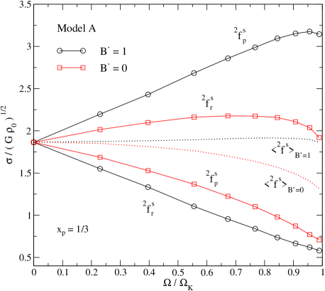
We first study a sequence of A models with $x_{\mathrm{p}}=1/3$, $\mathcal{R}=10^{3}$, and $\mathcal{\bar{B}}^{\prime}=-2$. According to equation (82), we would expect the pro- and retro-grade mode-branches to be exchanged compared to the $\mathcal{R}=0$ case. In Fig. 9 we show the ${}^{2}\rm{f}^{\mathrm{s}}$ mode for stellar models A rotating up to the mass shedding limit with $\mathcal{R}=0$ and $\mathcal{R}=10^{3}$, respectively. The results show that (82) describes the ${}^{2}\rm{f}^{\mathrm{s}}$ mode very well in the strong drag regime. We find that the scaling is quite accurate for stars up to $\Omega/\Omega_{K}=0.9$ (note that this analysis is not reported in Fig. 9). However, the agreement is not so good when the mutual friction vanishes. It seems that for $\mathcal{R}=0$ the effects of the centrifugal force becomes important for slower rotating models than in the $\mathcal{R}=10^{3}$ case. This behaviour is evident in Fig 9, when we consider the averaged frequency between the $m=2$ pro- and retro-grade modes, i.e. $\langle\sigma\rangle=\left(\sigma_{\rm{p}}+\sigma_{\rm{r}}\right)/2$.

However, we can take into account the effects of the centrifugal force on the average mode frequency and determine a connection between the superfluid f-mode frequencies in the strong and weak drag regimes. To this end, we define the mode deviation from its averaged value:

$$\Delta\sigma^{\mathrm{s}}=\sigma^{\mathrm{s}}-\langle\sigma^{\mathrm{s}}\rangle\,,$$ (83)

We then expect, from equation (82), that the following relation is valid:

$$\Delta\sigma^{\mathrm{s}}_{\mathcal{B}^{\prime}=1}\simeq\mathcal{\bar{B}^{\prime}}\Delta\sigma^{\mathrm{s}}_{\mathcal{B}^{\prime}=0}\,.$$ (84)

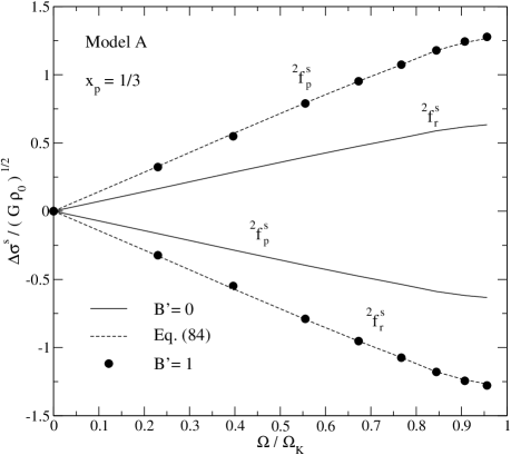
In the left panel of Fig. 9, we show the quantity $\Delta\sigma$ for the ${}^{2}\rm{f}^{\mathrm{s}}$ mode in the strong drag regime and for vanishing mutual friction. The results for the $\mathcal{R}=10^{3}$ case agree very well with the values obtained from equation (84).

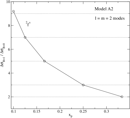
So far, we have studied a sequence of rotating stars with fixed proton fraction. Now, we test relation (84) by varying $x_{\mathrm{p}}$ and choosing the rotational model A2 with $\mathcal{R}=10^{3}$. The results in Fig. 10 show that the scaling of the ${}^{2}\rm{f}^{\mathrm{s}}$ mode with the proton fraction is well described by equation (84). However, when $x_{\mathrm{p}}=0.1$, there is a small difference between the numerical and analytical values. This effect might be due to the second order terms that we have neglected in the expansion (82). It is natural that these become important when the parameter $\mathcal{\bar{B}}^{\prime}$ is close to 10.

Let us now study the behaviour of the superfluid $l=m=2$ r-mode in the strong drag regime. Oscillations restored by the Coriolis force generate the class of inertial modes, which can be classified (by their parity) as axial-led or polar-led (Lockitch & Friedman, 1999). The ordinary r-modes form a sub-set that is purely axial in the slow-rotation limit. The superfluid problem is somewhat different in that a purely axial superfluid r-mode exists only in non-stratified stars. When composition gradients are present, the superfluid r-mode acquires a polar component and assumes the nature of a general inertial mode (Haskell et al., 2009).

For a constant density stellar model with $\mathcal{B}=0$, the frequency of the ${}^{2}\rm{r}^{\mathrm{s}}$ mode in the rotating frame is described by the following relation (Haskell et al., 2009):

$$\sigma^{\mathrm{s}}=\gamma_{\varepsilon}\mathcal{\bar{B}}^{\prime}\sigma^{\mathrm{o}}=\frac{2m\gamma_{\varepsilon}\mathcal{\bar{B}}^{\prime}\Omega}{l\left(l+1\right)}\,,$$ (85)

where $\sigma^{\mathrm{o}}$ is the frequency of the ordinary r-mode. In the case of $l=m=2$ we have $\sigma^{\mathrm{o}}_{\rm{r}}=2\Omega/3$. For compressible models, equation (85) approximately describes the frequency of the ${}^{2}\rm{r}^{\mathrm{s}}$ mode only for slowly rotating stars. In fact, when a star rotates rapidly the effects of $\mathcal{O}\left(\Omega^{3}\right)$ must be taken into account. In our time-evolutions, the rotational deformation of the star is completely described by the axisymmetric background. Meanwhile, in the slow-rotation approximation the equilibrium configuration remains spherical and the rotational effects on the spectrum are described by a perturbation expansion in $\Omega$. By using a slow-rotation approximation up to $\mathcal{O}\left(\Omega^{3}\right)$ and the Cowling approximation, Haskell et al. (2009) determined the frequency of the ${}^{2}\rm{r}^{\mathrm{o}}$ and ${}^{2}\rm{r}^{\mathrm{s}}$ modes in closed form. For the sequence of non-stratified A models with zero mutual friction, we have compared the r-mode frequencies of Haskell et al. (2009) with the spectrum extracted by the time-evolutions and found an agreement to better than $3\%$ up to models with $\Omega/\Omega_{K}\simeq 0.77$ (Passamonti et al., 2009a). For faster rotation, the slow-rotation approximation would require the calculation of terms of higher order than $\mathcal{O}\left(\Omega^{3}\right)$, which can be computationally prohibitive. In the strong drag regime, the effects of the higher order pertubative terms can become important even for relatively slowly rotating models, as a large value of $\mathcal{\bar{B}}^{\prime}$ increases the effective strength of the Coriolis force.

We study the superfluid r-modes of the rotating A models, where we fix the values of the entrainment and symmetry energy to zero, $\bar{\varepsilon}=\sigma=0$. The effects of these two parameters on the r-mode spectrum have already been studied by Passamonti et al. (2009a). In this paper, we focus on the effects of the mutual friction parameter $\mathcal{\bar{B}}^{\prime}$ by choosing $\mathcal{R}=10^{3}$ and consider four values of the proton fraction, namely $x_{\mathrm{p}}=2/5,\ 1/3,\ 1/4,\ 1/5$. The extraction of the r-mode frequencies from the time-evolutions requires longer simulations, as these modes are in the low-frequency regime. In order to save computational time, we adopt the Cowling approximation. In the right panel of Fig. 10 we show the ordinary ${}^{2}\rm{r}^{\mathrm{o}}$ and superfluid ${}^{2}\rm{r}^{\mathrm{s}}$ modes for different proton fractions. The ${}^{2}\rm{r}^{\mathrm{o}}$ mode has a retro-grade motion with respect to the star and is not affected by the parameter $x_{\mathrm{p}}$. In contrast, the ${}^{2}\rm{r}^{\mathrm{s}}$ mode depends strongly on $x_{\mathrm{p}}$ and has a pro-grade nature, as $\mathcal{\bar{B}}^{\prime}$ is negative.

Table 3: This table provides the fitting coefficients $c_{3},c_{5}$ of equation (86), and their errors $\Delta c_{3}$ and $\Delta c_{5}$, for the superfluid ${}^{2}\rm{r}^{\mathrm{s}}$ modes in the strong drag regime. The results correspond to the r-modes of four sequences of models A with $\mathcal{R}=10^{3}$ and $\varepsilon=\sigma=0$, and where the proton fraction takes the values shown in the first column. In the second column, we give the value of the parameter $\mathcal{\bar{B}}^{\prime}$. For the first two models, we do not show the values of $c_{5}$, as we fit the r-mode frequencies with $c_{5}=0$.

$x_{\mathrm{p}}$	$\mathcal{\bar{B}}^{\prime}$	$c_{3}$	$\Delta c_{3}$	$c_{5}$	$\Delta c_{5}$
			$\times 10^{-3}$	$\times 10^{-3}$	$\times 10^{-3}$
2/5	-1.5	0.11338	2.266
1/3	-2.0	0.01121	0.958
1/4	-3.0	-0.05599	0.948	6.275	0.233
1/5	-4.0	-0.05982	1.742	4.013	0.241

In order to understand the behaviour of the superfluid r-modes, we assume that for $\bar{\varepsilon}=\sigma=0$ the frequency of a counter-moving $l=m=2$ r-mode is described by the following relation;

$$\frac{\sigma^{\mathrm{s}}}{\sqrt{G\rho_{0}}}=\frac{2}{3}\mathcal{\bar{B}^{\prime}}\frac{\Omega}{\sqrt{G\rho_{0}}}+c_{3}\left(\mathcal{\bar{B}^{\prime}}\frac{\Omega}{\sqrt{G\rho_{0}}}\right)^{3}+c_{5}\left(\mathcal{\bar{B}^{\prime}}\frac{\Omega}{\sqrt{G\rho_{0}}}\right)^{5}+\mathcal{O}\left(\Omega\right)^{7}\,,$$ (86)

where the frequencies and angular velocities are expressed in dimensionless units, while $c_{3}$ and $c_{5}$ are two fitting parameters. The numerical spectrum, shown in Fig. 10, is well described by the first term of equation (86) only for slowest rotating models. For stars with $x_{\mathrm{p}}>1/4$ the agreement is good up to $\Omega/\Omega_{K}\simeq 0.4$, while for $x_{\mathrm{p}}\leq 1/4$ the range reduces to $\Omega/\Omega_{K}\leq 0.2$. In particular, we learn from the results in Fig. 10 that the mode pattern changes concavity for increasing values of $\mathcal{\bar{B}}^{\prime}$. This can be an effect of the $\mathcal{O}\left(\Omega^{3}\right)$ and $\mathcal{O}\left(\Omega^{5}\right)$ terms of equation (86). Therefore, we fit our numerical data with equation (86) and determine the parameters $c_{3}$ and $c_{5}$. For models with $x_{\mathrm{p}}>1/4$, a good fit can be determined by setting $c_{5}=0$ and calculating only the coefficient $c_{3}$. For the ordinary ${}^{2}\rm{r}^{\mathrm{o}}$ mode we obtain $c_{3}=0.4852\pm 0.0126$, while for the superfluid ${}^{2}\rm{r}^{\mathrm{s}}$ modes the results are given in Table 3. When the proton fraction is smaller, i.e. $x_{\mathrm{p}}\leq 1/4$, we must use the entire equation (86). The results of the corresponding fits are given in Table 3. In particular, when $x_{\mathrm{p}}\leq 1/4$ we note a sign change in the parameter $c_{3}$ that represents the concavity variation of the mode pattern.

Figure 11: This figure shows the waveform of the gravitational-wave signal for the C2 model with constant entrainment parameter $\bar{\varepsilon}=0.5$. We show the evolution of the two independent initial conditions ID-N (dashed-line) and ID-P (solid-line). The axis labels are in dimensionless units.

6.3 Glitch gravitational signal

We now turn to the gravitational-wave signal generated by initial axisymmetric configurations such that the protons and the neutrons rotate with a velocity lag. As discussed in Section 3.2, these configurations can be determined with the perturbative approach developed by Yoshida & Eriguchi (2004). We have already considered this problem (Sidery et al., 2010) in the context of pulsar glitches. The following discussion provides additional, more technical, details on these results.

Within the Yoshida & Eriguchi (2004) approach all the initial axisymmetric, non-corotating configurations of a corotating background can be constructed as a linear combination of two independent classes of initial data, see Section 3.2. In the first class, only the neutrons move relative to the corotating background, i.e. $\left(\delta\Omega_{\mathrm{n}},\delta\Omega_{\mathrm{p}}\right)=\left(1,0\right)$, while in the second class only the proton velocity is different from the corotating background, $\left(\delta\Omega_{\mathrm{n}},\delta\Omega_{\mathrm{p}}\right)=\left(0,1\right)$. We will refer to these two configurations as initial data N (ID-N) and P (ID-P), respectively. The initial mass density $\delta\rho_{x}$, chemical potential $\delta\tilde{\mu}_{\mathrm{x}}$ and gravitational potential $\delta\Phi$ can be directly determined from equations (25)–(26) for the two sets of initial data ID-N and ID-P. Meanwhile, for the velocity field perturbation we consider

$$\qquad\delta\mathbf{v}_{\mathrm{x}}=\delta\Omega_{\mathrm{x}}\,\left(\mathbf{\Omega}_{\mathrm{c}}\times\mathbf{r}\right)\,.$$ (87)

These solutions can be rescaled to any required glitch size if we note that the crust spin-up can be associated with the proton velocity lag $\delta\Omega_{\mathrm{p}}$. In fact, we expect an efficient coupling between the crust and the outer core protons due to the magnetic field, and we can then assume that the charged particles corotate. The rotational lag between superfluid neutrons and the protons can be estimated by considering angular momentum conservation:

$$\delta J=I_{\mathrm{n}}\delta\Omega_{\mathrm{n}}+I_{\mathrm{p}}\delta\Omega_{\mathrm{p}}+\left(\delta I_{\mathrm{n}}+\delta I_{\mathrm{n}}\right)\Omega_{\mathrm{c}}=0\,.$$ (88)

Here $J$ is the total angular momentum, $I_{\mathrm{x}}$ is the moment of inertia of each fluid constituent, and its perturbation $\delta I_{\mathrm{x}}$ is defined by

$$\delta I_{\mathrm{x}}=\int_{0}^{\mathbf{r}}\delta\rho_{\mathrm{x}}\,(r^{\prime}\sin\theta)^{2}d\mathbf{r^{\prime}}\,.$$ (89)

The initial relative velocity lag that describes a glitch is then given by

$$\delta\Omega_{\mathrm{p}} = \left.\frac{\Omega_{\mathrm{p}}-\Omega_{\mathrm{c}}}{\,\,\Omega_{\mathrm{c}}}\right|_{obs}\,,$$ (90)

$$\delta\Omega_{\mathrm{n}} = -\frac{1}{I_{\mathrm{n}}}\left(I_{\mathrm{p}}\delta\Omega_{\mathrm{p}}+\delta I\Omega_{\mathrm{c}}\right)\,,$$ (91)

where $\delta I=\delta I_{\mathrm{p}}+\delta I_{\mathrm{n}}$.

Figure 12: In this figure we illustrate the effect of the Cowling approximation on the gravitational signal. The background star is the C2 model with $\bar{\varepsilon}=0.5$, and the initial condition is that used for the glitch model, i.e. $\delta\Omega_{\mathrm{p}}=-10^{-6}$ and $\delta\Omega_{\mathrm{n}}=7.74\times 10^{-8}$. The waveforms are shown in the left panel and the PSD in the right panel. The signals determined in Cowling approximation and with gravitational potential perturbation are shown with dashed and solid lines respectively. In the right panel we note the effect of the Cowling approximation on the acoustic modes. For the initial data considered in this work, the Cowling approximation model generates a larger gravitational-wave amplitude than in the case when the gravitational potential perturbation is accounted for.

For each background model, we can evolve the two independent initial data sets ID-N and ID-P. If we consider a generic perturbation $\delta f$ for an arbitrary initial configuration, we can determine the evolution from the following linear combination:

$$\delta f=\delta f_{\rm{N}}\delta\Omega_{\mathrm{n}}+\delta f_{\rm{P}}\Omega_{\mathrm{p}}\,,$$ (92)

where $\delta f_{\rm{N}}$ and $\delta f_{\rm{P}}$ are the perturbation variables related to ID-N and ID-P, respectively.

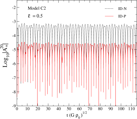
We have evolved the ID-N and ID-P configurations for the C2 model with $\bar{\varepsilon}=0.5$. In Fig. 11, we show a part of the time evolution of the quantity $A^{20}=A^{20}_{\mathrm{n}}+A^{20}_{\mathrm{p}}$ determined from the stress-formula (59). Actually, we show the dimensionless quantity $A^{20}_{\ast}=A^{20}/\left(G\rho_{0}^{2}R_{eq}^{2}\right)$ that is directly determined by the numerical code. For different values of the stellar parameters, the gravitational-wave amplitude can be calculated from equations (71) and (73). The initial data ID-N generates a gravitational signal that is about an order of magnitude larger than the ID-P initial data. We have studied stellar models with different proton fraction and noticed that the amplitude difference between the ID-N and ID-P initial data scales with the proton fraction of the background model. This is expected as the dynamics of the mass constituents generates the gravitational-wave signal.

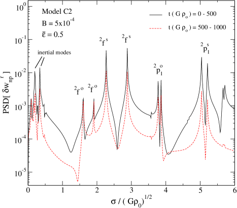
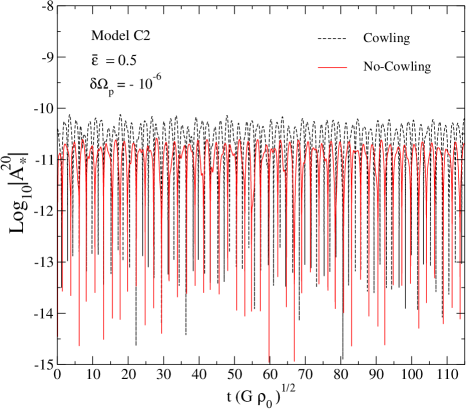
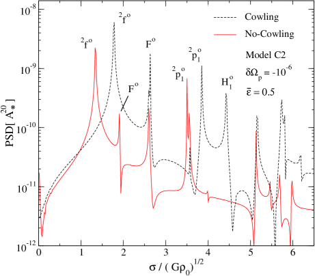
For the glitch initial data, we study the effect of the Cowling approximation on the gravitational-wave signal. To do this, we consider two simulations for the same model C2 and entrainment parameter $\bar{\varepsilon}=0.5$. The only difference is that, in one case we neglect the perturbation of the gravitational potential $\delta\Phi$. In Fig. 12, we show the time evolution of the quantity $A^{20}_{\ast}$ and the related Power Spectrum Density (PSD), which is defined as $\rm{PSD}(A^{20}_{\ast})=|\hat{A}^{20}_{\ast}|$. In the Cowling approximation, we extract the gravitational signal with the momentum formula (58), as the stress formula (59) is not well defined when $\delta\Phi=0$. From the results in the left panel of Fig. 12, we note that the Cowling approximation generates a signal that is about five times larger than the result when $\delta\Phi$ is included. Furthermore, as expected, the Cowling approximation introduces a deviation in the mode frequencies. This difference is evident in the right panel of Fig. 12, where the error is about $38\%$ for the fundamental quasi-radial mode ($\rm{F}^{\mathrm{o}}$), $32\%$ for the axisymmetric $l=2$ f-mode (${}^{2}\rm{f}^{\mathrm{o}}$), and $10\%$ for the first pressure mode (${}^{2}\rm{p}_{1}^{\mathrm{o}}$). These results agree well with the results of similar comparisons (Yoshida & Kojima, 1997; Yoshida & Eriguchi, 2001). Regarding the amplitude of the gravitational-wave signal, we find that the relative oscillation amplitude between the Cowling approximation and the full problem depends on the initial data. Hence, this result is not generic.

7 Conclusions and Discussion

We have studied the dynamics of superfluid rotating neutron stars, focussing on the nature of the oscillation spectrum, the effects of the mutual friction force on the oscillations and the hydrodynamic spin-up phase of pulsar “glitches”. Adopting the Newtonian two-fluid model, we evolved in time the perturbed dynamical equations on axisymmetric equilibrium configurations. This approach allows us to derive the spectrum of axisymmetric and non-axisymmetric oscillation modes of stellar models that rotate up to the mass shedding limit. In this work, we have improved on previous studies by including the gravitational perturbation and the mutual friction force. The spectrum is then determined with a better accuracy, as we no longer use the Cowling approximation (Passamonti et al., 2009a). From the computational point of view, we have to solve the perturbed Poisson equation together with the linearised momentum and mass conservation equations. We have numerically evolved the hyperbolic equations with a Mac-Cormack algorithm, while the elliptic equation for the gravitational potential is solved at each time step with a spectral method.

In our current model the rotating background models are pure fluid, i.e. without an elastic crust region, neutrons and protons corotate and are in $\beta$-equilibrium. In superfluid stars, the co- and counter-phase motion of the two fluid constituents can be coupled by composition gradients and this influences the dynamics. In order to consider this effect we have studied two simple polytropic equations of state that generate distinct sequences of stratified and non-stratified rotating stars. These background models are simplistic, and we must improve on this aspect if we want to decode the complexity of astrophysical observations. Certainly, we must add an elastic crust to the model and relax the co-rotation assumption between the two fluids. If we want to use more realistic equations of state we also need to translate the model to General Relativity. We are currently working on all these issues.

In neutron stars, the mutual friction force may have both dissipative and non-dissipative effects. The dissipative part of the force, which is dominant in the weak drag regime, mainly damps an oscillation mode. Meanwhile, the non-dissipative term dominates in the strong drag regime, essentially modifying the oscillation spectrum. We have studied the two drag regimes and showed that our numerical code effectively reproduces the mutual friction damping of the two-fluid relative motion. For non-stratified stars, the co- and counter-moving degrees of freedom are uncoupled and only the superfluid modes are damped. When the stellar model is stratified, the damping affects also the ordinary modes. The accuracy of our numerical code has also been tested in Sidery et al. (2010), where determined the glitch spin-up time and compared it to a simple analytic formula. However, we are not yet able to extract (with useful precision) the mutual friction damping time of individual oscillation modes from our numerical evolutions. More work is needed to establish to what extent one should expect to do this within our computational framework. For the strong drag regime, we have studied the effect of the mutual friction and composition variation on the rotational splitting of the superfluid $l=m=2$ f-mode and on the frequencies of the $l=m=2$ superfluid r-mode. The main effect is a change of propagation direction of the modes with respect to the background rotation. A mode that is pro-grade (retro-grade) in the weak drag regime may become retro-grade (pro-grade) in the strong drag regime. We have determined the numerical frequencies of the f- and r-modes for the rotating sequence of non-stratified stellar models and provided simple empirical expressions based on the numerical data. For constant mutual friction parameters, the non-axisymmetric splitting of the superfluid f-mode and the r-mode frequencies depends on the inverse of the proton fraction.

Finally, we provided relevant technical details for the hydrodynamical models for pulsar glitches discussed by Sidery et al. (2010). The initial conditions for the glitch evolutions describe two fluids that rotate with a small velocity lag. These configurations were been determined using a perturbative approach first introduced by Yoshida & Eriguchi (2004). We extended this method to implement different EoS and consider non-corotating initial configurations that conserve the mass of each fluid constituent. Moreover, we derived the detailed quadrupole gravitational extraction formulae for $l=2$ oscillation modes of a superfluid star. We determined the perturbative expressions for the momentum and stress formulae that can be used to improve the numerical extraction of the gravitational-wave signal (reducing the order of the time derivative of the standard quadrupole formula). We determined the gravitational-wave strain for the two independent initial glitch configurations that are obtained with the Yoshida & Eriguchi (2004) approach. For a given background rotation, these results can be used to estimate the gravitational signal for any glitch size. Furthermore, we have showed the effect of the Cowling approximation on the glitch gravitational-wave strain and the oscillation spectrum.

With the progress described in this paper, our programme of studying superfluid neutron star dynamics by time-evolutions of the linearised equations has reached the point where we need to add key physics to the model. The natural step would be to account for the elastic neutron star crust with the expected interpenetrating neutron superfluid. This requires us to change the computational framework somewhat, as it is natural to discuss the elasticity in term of Lagrangian perturbation theory. Moreover, we need to address various issues associated with vortex pinning by the crust nuclei. This problem requires additional force contributions at the level of individual vortices, and we need to develop a suitable smooth-averaged hydrodynamics description if we want to make progress. We are currently working on both these issues. It would also be relevant to extend our models to general relativity. This is essential if we want to be able to use realistic supranuclear equations of state. As long as we make use of the relativistic analogue of the Cowling approximation this generalisation should be straightforward, but if we want to account for the dynamics of spacetime the problem becomes much more involved. If we want to consider realistically “layered” neutron stars we also need to improve our understanding of the different phase-transitions, e.g. in the vicinity of the critical density/temperature for the onset of superfluidity, and how these regions affect the large scale dynamics. We face a number of challenging questions, but there is no reason why we should not be able to resolve the relevant issues and progress towards the construction of realistic dynamical neutron star models.

Appendix A GW extraction

In this Appendix we determine the momentum formula (65) and the stress formula (66) for the $(l,m)=(2,2)$ gravitational signal. For the axisymmetric $(l,m)=(2,0)$ case, we have used the perturbative version of the momentum and stress formulae used by Finn & Evans (1990).

The aim is to reduce the order of the time derivatives in the quadrupole gravitational-wave formula. To do this we consider the quantity (63):

$$A^{22}\equiv\frac{d^{2}}{dt^{2}}\int d\mathbf{r}\,\delta\rho\,r^{2}Y_{22}^{\ast}\,.$$ (93)

With the use of the mass conservation equations of each fluid component:

$$\partial_{t}\rho_{\mathrm{x}}+\nabla_{i}\left(\rho_{\mathrm{x}}v_{\mathrm{x}}^{i}\right)=0\,,$$ (94)

we can determine the momentum-formula where only a first order time derivative appears. When we perturb equation (94) and introduce it in (93) we obtain:

$$A^{22} = \frac{d^{2}}{dt^{2}}\int d\mathbf{r}\,\delta\rho\,r^{2}\,Y_{22}^{\ast}=\sum_{\mathrm{x}}\frac{d}{dt}\int d\mathbf{r}\,\partial_{t}\left(\delta\rho_{\mathrm{x}}\right)\,r^{2}\,Y_{22}^{\ast}=-\sum_{\mathrm{x}}\frac{d}{dt}\int d\mathbf{r}\,\nabla_{i}\delta\left(\rho_{\mathrm{x}}v_{\mathrm{x}}^{i}\right)r^{2}\,Y_{22}^{\ast}$$ (95)

$$= \sum_{\mathrm{x}}\frac{d}{dt}\int d\mathbf{r}\,\,\delta\left(\rho_{\mathrm{x}}v^{k}_{\mathrm{x}}\right)\nabla_{k}\left(r^{2}\,Y_{22}^{\ast}\right)\,.$$

where in the last step we have used the Gauss Theorem. After some calculation, equation (95) leads to the expression (65).

With a similar method, we can determine the stress-formula and eliminate the time derivatives from the quadrupole formula. In this case, we must use the momentum conservation equation that for a superfluid component is given by

$$\partial_{t}\left(\rho_{\mathrm{x}}p^{\mathrm{x}}_{i}\right)+\nabla_{k}\left(\rho_{\mathrm{x}}v_{\mathrm{x}}^{i}p^{\mathrm{x}}_{i}\right)+\rho_{\mathrm{x}}\nabla_{i}\tilde{\mu}_{\mathrm{x}}+\rho_{\mathrm{x}}\nabla_{i}\Phi+\rho_{\mathrm{x}}\varepsilon_{\mathrm{x}}w_{k}^{\mathrm{y}\mathrm{x}}\nabla_{i}v_{\mathrm{x}}^{k}=0\,,$$ (96)

where the momentum of the fluid component is defined as follows:

$$p_{i}^{\mathrm{x}}=v_{i}^{\mathrm{x}}+\varepsilon_{\mathrm{x}}w_{i}^{\mathrm{y}\mathrm{x}}\,.$$ (97)

For a two-fluid model with neutron and proton as components, the total momentum equation is then given by the following expression:

$$\partial_{t}\left(\rho_{\mathrm{n}}v^{\mathrm{n}}_{i}+\rho_{\mathrm{p}}v^{\mathrm{p}}_{i}\right)=-\nabla_{k}\left(\rho_{\mathrm{n}}v_{\mathrm{n}}^{k}p^{\mathrm{n}}_{i}+\rho_{\mathrm{p}}v_{\mathrm{p}}^{k}p^{\mathrm{p}}_{i}\right)-\nabla_{i}\Psi-\frac{1}{4\pi G}\nabla^{k}\left(\nabla_{k}\Phi\nabla_{i}\Phi-\frac{\delta_{ik}}{2}\nabla_{j}\Phi\nabla^{j}\Phi\right)\,,\\$$ (98)

where we have used the definition of the the generalized pressure (Prix, 2004):

$$\nabla\Psi=\rho_{\mathrm{n}}\nabla\tilde{\mu}_{\mathrm{n}}+\rho_{\mathrm{p}}\nabla\tilde{\mu}_{\mathrm{p}}-\frac{1}{2}\rho_{\mathrm{x}}\varepsilon_{\mathrm{x}}\nabla\left(w_{\mathrm{p}\mathrm{n}}^{2}\right)\,,$$ (99)

and we have re-written the gravitational potential term by using the Poisson equation:

$$\rho\nabla_{i}\Phi=\frac{1}{4\pi G}\nabla^{k}\left(\nabla_{k}\Phi\nabla_{i}\Phi-\frac{\delta_{ik}}{2}\nabla_{j}\Phi\nabla^{j}\Phi\right)\,.$$ (100)

Perturbing equation (98) and considering a corotating equilibrium configuration, i.e. $w_{\mathrm{n}\mathrm{p}}=0$, we obtain:

$$\frac{\partial}{\partial t}\,\delta\left(\rho_{\mathrm{n}}v^{\mathrm{n}}_{i}+\rho_{\mathrm{p}}v^{\mathrm{p}}_{i}\right)=-\nabla_{k}\delta\left(\rho_{\mathrm{n}}v_{\mathrm{n}}^{k}p^{\mathrm{n}}_{i}+\rho_{\mathrm{p}}v_{\mathrm{p}}^{k}p^{\mathrm{p}}_{i}\right)-\nabla_{i}\delta P-\frac{1}{4\pi G}\nabla^{k}\delta\left(\nabla_{k}\Phi\nabla_{i}\Phi-\frac{\delta_{ik}}{2}\nabla_{j}\Phi\nabla^{j}\Phi\right)\,,\\$$ (101)

where now for corotating background the pressure perturbation is given by

$$\nabla\delta P=\delta\left(\rho_{\mathrm{n}}\nabla\tilde{\mu}_{\mathrm{n}}+\rho_{\mathrm{p}}\nabla\tilde{\mu}_{\mathrm{p}}\right)\,.$$ (102)

We can now introduce equation (101) into equation (95) and use the Gauss theorem. We obtain:

$$\frac{d^{2}}{dt^{2}}\int d\mathbf{r}\,\delta\rho\,r^{2}\,Y_{22}^{\ast}=\int d\mathbf{r}\,\delta\left(\rho_{\mathrm{n}}v_{\mathrm{n}}^{k}p^{i}_{\mathrm{n}}+\rho_{\mathrm{p}}v_{\mathrm{p}}^{k}p^{i}_{\mathrm{p}}+\frac{1}{4\pi}\nabla^{k}\Phi\nabla^{i}\Phi\right)\nabla_{i}\nabla_{k}\left(r^{2}\,Y_{22}^{\ast}\right)$$ (103)

where both the pressure and the last term of equation (101) vanish, as $\nabla^{2}\left(r^{2}\,Y_{22}^{\ast}\right)=0$. After some further calculation, we can derive equation (66) from (103).

References

- Alpar et al. (1984) Alpar M. A., Langer S. A., Sauls J. A., 1984, ApJ, 282, 533
- Andersson & Comer (2001) Andersson N., Comer G. L., 2001, MNRAS, 328, 1129
- Andersson & Comer (2006) Andersson N., Comer G. L., 2006, Classical and Quantum Gravity, 23, 5505
- Andersson et al. (2004) Andersson N., Comer G. L., Grosart K., 2004, MNRAS, 355, 918
- Andersson et al. (2002) Andersson N., Comer G. L., Langlois D., 2002, Phys. Rev. D, 66, 104002
- Andersson et al. (2009) Andersson N., Ferrari V., Jones D. I., Kokkotas K. D., Krishnan B., Read J., Rezzolla L., Zink B., 2009, preprint (arXiv:0912.0384)
- Andersson et al. (2009) Andersson N., Glampedakis K., Haskell B., 2009, Phys. Rev. D, 79, 103009
- Andersson et al. (2009) Andersson N., Glampedakis K., Samuelsson L., 2009, MNRAS, 396, 894
- Andersson & Kokkotas (1998) Andersson N., Kokkotas K. D., 1998, MNRAS, 299, 1059
- Benhar et al. (2004) Benhar O., Ferrari V., Gualtieri L., 2004, Phys. Rev., D70, 124015
- Chamel (2008) Chamel N., 2008, MNRAS, 388, 737
- Colaiuda et al. (2009) Colaiuda A., Beyer H., Kokkotas K. D., 2009, MNRAS, 396, 1441
- Cowling (1941) Cowling T. G., 1941, MNRAS, 101, 367
- Dimmelmeier et al. (2006) Dimmelmeier H., Stergioulas N., Font J. A., 2006, MNRAS, 368, 1609
- Finn & Evans (1990) Finn L. S., Evans C. R., 1990, ApJ, 351, 588
- Flanagan & Hughes (1998) Flanagan É. É., Hughes S. A., 1998, Phys. Rev. D, 57, 4535
- Gaertig & Kokkotas (2009) Gaertig E., Kokkotas K. D., 2009, Phys. Rev. D, 80, 064026
- Glampedakis et al. (2010) Glampedakis K., Andersson N., Samuelsson L., 2010, preprint (arXiv:1001.4046)
- Grandclément & Novak (2009) Grandclément P., Novak J., 2009, Living Rev. in Relativity, 12
- Hachisu (1986) Hachisu I., 1986, ApJSS, 61, 479
- Haskell et al. (2009) Haskell B., Andersson N., Passamonti A., 2009, MNRAS, 397, 1464
- Jones et al. (2002) Jones D. I., Andersson N., Stergioulas N., 2002, MNRAS, 334, 933
- Lee (1995) Lee U., 1995, A&A, 303, 515
- Lee & Yoshida (2003) Lee U., Yoshida S., 2003, ApJ, 586, 403
- Lindblom & Mendell (1995) Lindblom L., Mendell G., 1995, ApJ, 444, 804
- Lindblom & Mendell (2000) Lindblom L., Mendell G., 2000, Phys. Rev. D, 61, 104003
- Lockitch & Friedman (1999) Lockitch K. H., Friedman J. L., 1999, ApJ, 521, 764
- Mendell (1991a) Mendell G., 1991a, ApJ, 380, 515
- Mendell (1991b) Mendell G., 1991b, ApJ, 380, 530
- Nagar & Diaz (2004) Nagar A., Diaz G., 2004, in Proceedings of the 27th Spanish Relativity Meeting (ERE 2003): Gravitational Radiation, Alicante, Spain, (University of Alicante, Alicante, Spain)
- Papaloizou & Pringle (1980) Papaloizou J. C., Pringle J. E., 1980, MNRAS, 190, 43
- Passamonti et al. (2009a) Passamonti A., Haskell B., Andersson N., 2009a, MNRAS, 396, 951
- Passamonti et al. (2009b) Passamonti A., Haskell B., Andersson N., Jones D. I., Hawke I., 2009b, MNRAS, 394, 730
- Passamonti et al. (2007) Passamonti A., Stergioulas N., Nagar A., 2007, Phys. Rev. D, 75, 084038
- Prix (2004) Prix R., 2004, Phys. Rev. D, 69, 043001
- Prix et al. (2002) Prix R., Comer G. L., Andersson N., 2002, A&A, 381, 178
- Prix & Rieutord (2002) Prix R., Rieutord M., 2002, A&A, 393, 949
- Samuelsson & Andersson (2007) Samuelsson L., Andersson N., 2007, MNRAS, 374, 256
- Samuelsson & Andersson (2009) Samuelsson L., Andersson N., 2009, Classical and Quantum Gravity, 26, 155016
- Sidery et al. (2010) Sidery T., Passamonti A., Andersson N., 2010, MNRAS, pp 554–+
- Stergioulas et al. (2004) Stergioulas N., Apostolatos T. A., Font J. A., 2004, MNRAS, 352, 1089
- Thorne (1980) Thorne K. S., 1980, Reviews of Modern Physics, 52, 299
- Watts & Strohmayer (2007) Watts A. L., Strohmayer T. E., 2007, Ap&SS, 308, 625
- Yoshida & Eriguchi (2001) Yoshida S., Eriguchi Y., 2001, MNRAS, 322, 389
- Yoshida & Eriguchi (2004) Yoshida S., Eriguchi Y., 2004, MNRAS, 347, 575
- Yoshida & Kojima (1997) Yoshida S., Kojima Y., 1997, MNRAS, 289, 117
- Zerilli (1970) Zerilli F. J., 1970, Phys. Rev. Lett., 24, 737