Multiplication of sparse Laurent polynomials and Poisson series on modern hardware architectures

Abstract

In this paper we present two algorithms for the multiplication of sparse Laurent polynomials and Poisson series (the latter being algebraic structures commonly arising in Celestial Mechanics from the application of perturbation theories). Both algorithms first employ the Kronecker substitution technique to reduce multivariate multiplication to univariate multiplication, and then use the schoolbook method to perform the univariate multiplication. The first algorithm, suitable for moderately-sparse multiplication, uses the exponents of the monomials resulting from the univariate multiplication as trivial hash values in a one dimensional lookup array of coefficients. The second algorithm, suitable for highly-sparse multiplication, uses a cache-optimised hash table which stores the coefficient-exponent pairs resulting from the multiplication using the exponents as keys.

Both algorithms have been implemented with attention to modern computer hardware architectures. Particular care has been devoted to the efficient exploitation of contemporary memory hierarchies through cache-blocking techniques and cache-friendly term ordering. The first algorithm has been parallelised for shared-memory multicore architectures, whereas the second algorithm is in the process of being parallelised.

We present benchmarks comparing our algorithms to the routines of other computer algebra systems, both in sequential and parallel mode.

1 Introduction

The application of perturbation theories for non-linear differential equations in Celestial Mechanics is a task traditionally associated with cumbersome yet simple operations on basic algebraic structures. Modern applications of perturbative methods to the problem of the long-term stability of the Solar System, for instance, lead to series expansions whose number of terms is in the order of $10^{5}-10^{6}$ [23, 14]. It is then not surprising that astronomers and celestial mechanicians have sought – since the dawn of the digital age – to fully exploit the power and reliability of computers in this domain, producing a vast amount of literature on specialised (as opposed to general-purpose) algebraic manipulators [16, 7, 19, 20, 29, 6, 3, 9, 28, 2, 18, 13].

Typically, perturbative methods in Celestial Mechanics require the ability to manipulate symbolically algebraic structures known as Poisson series [30], consisting of Fourier series having Laurent polynomials as coefficients:

$$\sum_{j_{1}\ldots j_{m}}\sum_{i_{1}\ldots i_{n}}C_{i_{1}\ldots i_{n},j_{1}\ldots j_{m}}x_{1}^{i_{1}}\cdots x_{n}^{i_{n}}\\ \begin{matrix}\cos\\ \sin\end{matrix}\left(j_{1}y_{1}+\ldots+j_{m}y_{m}\right).$$ (1)

Here the symbolic variables are denoted by $x$ and $y$, while $i$ and $j$ are integer indices and $C$ is a numerical coefficient. The mathematical operations to be performed on such objects are usually elementary. E.g., the computation of normal forms using the Lie series technique, a popular methodology in Celestial Mechanics, requires the operations of addition, subtraction, multiplication, differentiation and integration [10].

The most taxing operation to be performed on Poisson series, which also forms the basis for more complicated operations such as Taylor expansions, is series multiplication. In this paper we present two algorithms for the multiplication of sparse Laurent polynomials and Poisson series which employ the technique of Kronecker substitution and whose implementation seeks to maximise performance on modern computer hardware architectures.

2 Kronecker substitution

Kronecker substitution, first described in [22], is a methodology that allows to reduce multivariate polynomial multiplication to univariate multiplication, and it can be intuitively understood with the aid of a simple table laying out the monomials in reverse lexicographic order. The representation for three variables $x$, $y$ and $z$, and up to the third power in each variable is displayed in Table 1.

$z$	$y$	$x$	Code
0	0	0	0
0	0	1	1
0	0	2	2
0	0	3	3
0	1	0	4
0	1	1	5
0	1	2	6
0	1	3	7
0	2	0	8
$\ldots$	$\ldots$	$\ldots$	$\ldots$
3	3	3	63

Table 1: Kronecker substitution for a 3-variate polynomial up to the third power in each variable.

The column of codes is obtained by a simple enumeration of the exponents’ multiindices. It can be noted how in certain cases the addition of multiindices (and hence the multiplication of the corresponding monomials) maps to the addition of their codified representation. For instance:

$$c\left(\left[0,0,3\right]\right)+c\left(\left[0,1,0\right]\right)=3+4=7=\\ =c\left(\left[0,1,3\right]\right)=c\left(\left[0,0,3\right]+\left[0,1,0\right]\right),$$ (2)

where we have noted with $c=c\left(\mathbf{e}\right)$ the function that codifies a multiindex vector of exponents $\mathbf{e}$. An inspection of Table 1 promptly suggests that for an $m$-variate polynomial up to exponent $n$ in each variable, $c$’s effect is equivalent to a scalar product between the multiindices vectors and a constant coding vector $\mathbf{c}$ defined as

$$\mathbf{c}=\left[\left(n+1\right)^{m-1},\left(n+1\right)^{m-2},\ldots,n+1,1\right],$$ (3)

so that

$$c\left(\mathbf{e}\right)=\mathbf{c}\cdot\mathbf{e},$$ (4)

and eq. (2) can be generalised as

$$\mathbf{c}\cdot\left(\mathbf{e}_{1}+\mathbf{e}_{2}\right)=\mathbf{c}\cdot\mathbf{e}_{1}+\mathbf{c}\cdot\mathbf{e}_{2}.$$ (5)

While this equation is valid in general due to the distributivity of scalar multiplication, the codification of a multiindex will produce a unique code only if the multiindex is representable within the representation defined by $\mathbf{c}$.

This simple example shows how Kronecker substitution constitutes an addition-preserving homomorphism between the space of integer vectors whose elements are bound in a finite range and a finite subset of integers. Since the addition of codes maps to the addition of multiindices, the codes can be seen as exponents of a univariate polynomial.

For use with Laurent polynomials and Poisson series, Kronecker substitution can be conveniently generalised in the following way:

• we can consider variable codification, i.e., each element of the multiindex has its own range of variability;

• we can extend the validity of the codification to negative integers.

The first generalisation allows to compact the range of the codes. If, for instance, the exponent of variable $x$ in the example above varies only from 0 to 1 (instead of varying from 0 to 3 like for $y$ and $z$), we can avoid codes that we know in advance will be associated to nonexisting monomials (i.e., all those in which $x$’s exponent is either 2 or 3). The second generalisation derives from the fact that under an appropriate extension of the coding vector it is possible to change $\mathbf{e}_{2}$’s sign in eq. (5) retaining the validity of the homomorphism, allowing thus to apply Kronecker substitution to the multiplication of Poisson series. Poisson series multiplication, indeed, requires the ability to deal also with negative exponents (since by definition Laurent polynomials may have terms of negative degree); additionally, the trigonometric multipliers (i.e., the $j$ indices in eq. (1)) transform under multiplication according to the following elementary trigonometric formulas, which imply the need to be able to subtract vectors of trigonometric multipliers:

$$\begin{gathered}\cos\alpha\cdot\cos\beta=\cos\left(\alpha-\beta\right)+\cos\left(\alpha+\beta\right),\\ \cos\alpha\cdot\sin\beta=\sin\left(\alpha+\beta\right)-\sin\left(\alpha-\beta\right),\\ \sin\alpha\cdot\cos\beta=\sin\left(\alpha-\beta\right)+\sin\left(\alpha+\beta\right),\\ \sin\alpha\cdot\sin\beta=\cos\left(\alpha-\beta\right)-\cos\left(\alpha+\beta\right).\end{gathered}$$ (6)

Table 2 shows the generalised Kronecker substitution for a multivariate Laurent polynomial (and Poisson series) in which the exponents (and trigonometric multipliers) vary on different ranges, possibly assuming negative values.

$x_{m-1}$	$\ldots$	$x_{1}$	$x_{0}$	Code
$e_{m-1,\min}$	$\ldots$	$e_{1,\min}$	$e_{0,\min}$	$0$
$e_{m-1,\min}$	$\ldots$	$e_{1,\min}$	$1+e_{0,\min}$	$1$
$\ldots$	$\ldots$	$\ldots$	$\ldots$	$\ldots$
$e_{m-1,\min}$	$\ldots$	$e_{1,\min}$	$e_{0,\max}$	$e_{0,\max}-e_{0,\min}$
$e_{m-1,\min}$	$\ldots$	$1+e_{1,\min}$	$e_{0,\min}$	$1+e_{0,\max}-e_{0,\min}$
$e_{m-1,\min}$	$\ldots$	$1+e_{1,\min}$	$1+e_{0,\min}$	$2+e_{0,\max}-e_{0,\min}$
$e_{m-1,\min}$	$\ldots$	$1+e_{1,\min}$	$2+e_{0,\min}$	$3+e_{0,\max}-e_{0,\min}$
$\ldots$	$\ldots$	$\ldots$	$\ldots$	$\ldots$

Table 2: Generalised Kronecker substitution for an $m$-variate Laurent polynomial (or Poisson series) in which each exponent (or trigonometric multiplier) varies on a different range.

If we define:

$$\mathbf{e} = \left(e_{0},e_{1},\ldots,e_{m-1}\right),$$ (7)

$$\mathbf{e}_{\min/\max} = \left(e_{0,\min/\max},e_{1,\min/\max},\ldots,\right.$$ (8)

$$\left.e_{m-1,\min/\max}\right),$$

$$w_{k} = 1+e_{k,\max}-e_{k,\min},$$ (9)

$$\mathbf{c} = \left(1,w_{0},w_{0}w_{1},w_{0}w_{1}w_{2},\ldots,\vphantom{\Pi_{k=0}^{m-2}w_{k}}\right.$$ (10)

$$\left.\Pi_{k=0}^{m-2}w_{k}\right),$$

$$\chi = \mathbf{c}\cdot\mathbf{e}_{\min},$$ (11)

it is easy to show that the code of the generic multiindex $\mathbf{e}$ is obtained by

$$c\left(\mathbf{e}\right)=\mathbf{c}\cdot\mathbf{e}-\chi.$$ (12)

To recap, this generalisation of the Kronecker substitution technique allows to reduce the multiplication of two multivariate Poisson series and Laurent polynomials to the multiplication of two univariate polynomials.

3 The algorithms

In most applications of practical interest, the univariate polynomials resulting from the application of Kronecker substitution are sparse. E.g., the Fateman benchmark, presented in §5 and described as a dense benchmark in [25], after being reduced to a univariate multiplication features roughly $1$ non-null monomial every $300$ in the univariate factors. Series arising in the context of Celestial Mechanics are usually sparser. Because of this, asymptotically fast algorithms for dense multiplication, such as FFT and Karatsuba, are not usually employed in Celestial Mechanics (see also the discussion in [11]). The algorithms described in this paper thus employ schoolbook (aka ordinary) multiplication: each monomial of the first univariate polynomial factor is multiplied by all the monomials of the second factor.

Desirable properties of a multiplication algorithm for Celestial Mechanics applications include:

• the ability to operate on multiple types of numerical coefficients (e.g., reals, rationals, integers, both in machine precision and multiprecision, complex numbers, intervals);

• the ability to efficiently truncate multiplication.

The second requirement stems from the observation that the number of terms of the series involved in many practical calculations tends to explode during multiplication, if not controlled properly. Typical truncation criterions concern quantities such as the absolute value of the numerical coefficients, the minimum exponents of one or more polynomial variables and the order of the Fourier harmonics (see the discussion in [26], Chapter 2, Section 3).

In any case, in order to truncate efficiently (i.e., without having to compute a term to discard it afterwards), a truncation criterion may define an ordering over the terms of the series being multiplied. This way, while multiplying one monomial of the first factor and iterating over the monomials of the second factor, it may be possible to skip all monomial-by-monomial multiplications from a certain point onwards. The multiplication algorithm, hence, should ideally be flexible enough to allow for this kind of truncation methodology without a negative impact on performance.

3.1 Moderately-sparse multiplication

The first algorithm we present is very simple and suitable for moderately-sparse multiplication. The two univariate polynomial factors are represented as vectors of coefficient-exponent pairs (a representation often referred to as sparse distributed). The resulting univariate polynomial is represented instead as a vector of coefficients, with the positional index of each coefficient implicitly encoding the corresponding exponent (a dense distributed representation). This vector of coefficients is initialised with null values.

Each monomial-by-monomial multiplication generates a coefficient, which is added to the coefficient in the output vector at the positional index equal to the sum of the exponents of the monomial factors (see Figure 1). In case of Poisson series multiplication, the same coefficient is also added to the coefficient at the positional index equal to the subtraction of the exponents of the monomial factors (as per eqs. (6)). The exponents of the monomials resulting from the multiplication, in other words, are used as trivial (and perfect) hash values for accumulation in a lookup array of coefficients.

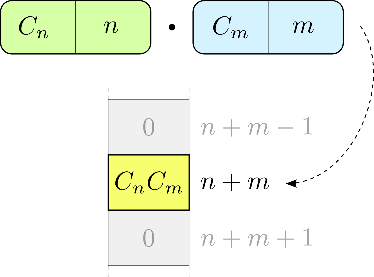
Figure 1: Moderately-sparse multiplication: the multiplication of two terms $\left(C_{n},n\right)$ and $\left(C_{m},m\right)$ of the univariate polynomial factors (where $n$ and $m$ are the exponents to which coefficients $C_{n}$ and $C_{m}$ are associated) produces coefficient $C_{n}C_{m}$, which is stored in the output array of coefficients at position $n+m$.

The practical performance of this algorithm crucially depends on two optimisations related to cache memory:

• cache blocking: the two polynomial factors are subdivided logically into blocks, and, rather than iterating over all the monomials of the second factor having fixed a monomial in the first one (in a doubly-nested for loop fashion), multiplication is performed block-by-block. The effect is the same as if the two factors were subdivided into smaller polynomials to be multiplied separately;

• monomial ordering: the two polynomial factors are sorted in ascending order according to the degree of the monomials.

The combined effect of these optimisations is a cache-friendly memory access pattern which promotes temporal and spatial locality of reference through:

1. sequential writes into the output coefficient vector, by virtue of the monomial ordering,

2. short-term reuse of data already present into the cache memory, by virtue of cache blocking.

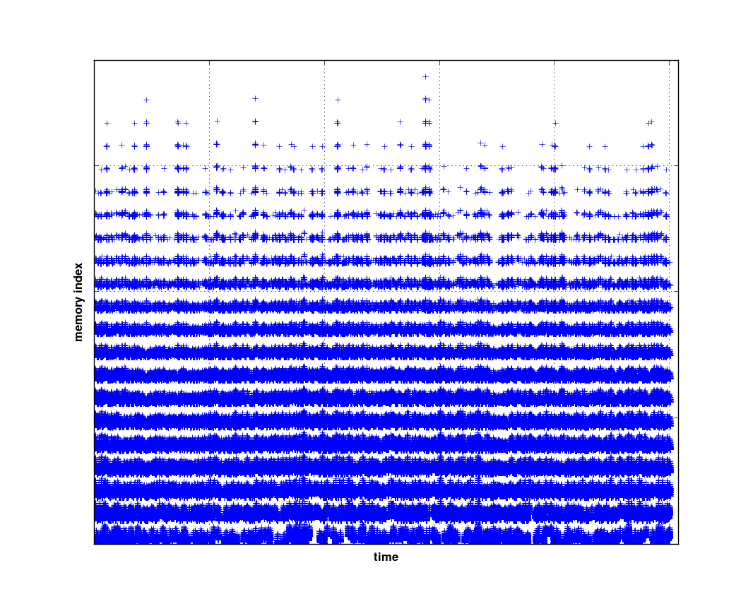
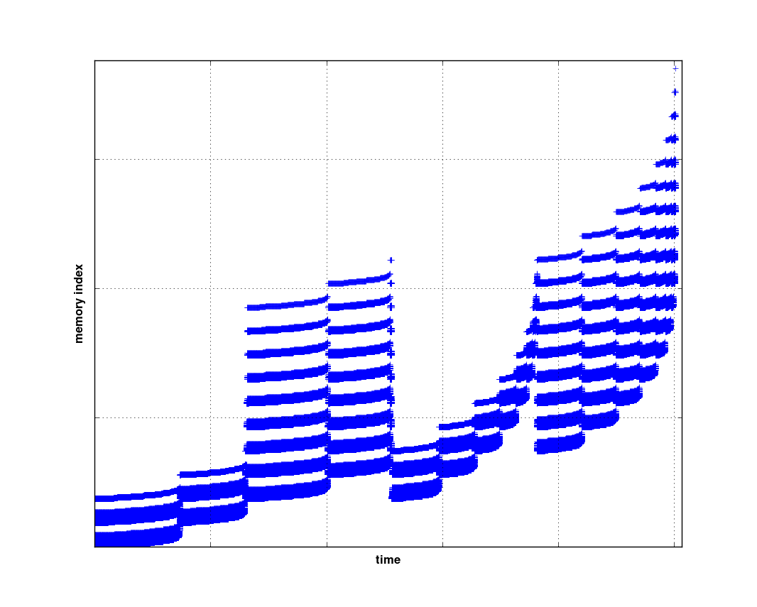
Figure 2: Typical memory access patterns for moderately-sparse multiplication, with (right) and without (left) cache-blocking and term ordering optimisation. The $x$ axis displays the time at which the memory write is performed in the output coefficient vector, the $y$ axis displays its location within the vector.

A typical memory access pattern for moderately-sparse multiplication is displayed in Figure 2.

These optimisations cope well also when a different monomial ordering is required by the truncation criterion. Indeed, to retain much of the cache-friendly memory access pattern, it is enough to first order the monomials according to the degree and then reorder within each block the monomials according to the order requested by the truncation criterion.

3.2 Highly-sparse multiplication

In case of highly-sparse multiplication, the algorithm described above may not be applicable for the following reasons:

• the output coefficient array would occupy much too memory storage,

• the high sparsity would result in a large array whose initialisation overhead would outweigh the time spent in the actual multiplication.

Such occurrences are detectable through an analysis of the densities of the univariate polynomial factors.

The algorithm we have adopted to cope with the highly-sparse case is based on hashing techniques, and it essentially replaces the output coefficient array of the first algorithm with a cache-friendly hash table. Our design is just one possibility of cache-friendly hash table: other designs, including cuckoo hashing [27] and hopscotch hashing [17] (but also linear probing [21]) may be effective too.

The hash table is implemented as a contiguous memory area of size $n$ logically subdivided into $N$ adjacent buckets of maximum size $m=n/N$. The buckets store coefficient-exponent pairs (i.e., in a sparse distributed representation). The exponents of the monomials resulting from the multiplication of the univariate polynomial factors are used, after modulo reduction, as hash values to accumulate the monomials into the hash table. E.g., when a monomial with exponent $e$ is produced during multiplication, its hash value $h$ is computed,

$$h=e\bmod{N},$$ (13)

and the monomial is inserted into the $h$-th bucket (see Figure 3). If the bucket already contains a term with the same exponent $e$, then the coefficient of the incoming monomial is added to the existing one. Otherwise the monomial is appended at the end of the bucket. Since the maximum size of the buckets is $m$, insertion of a new monomial can fail when a bucket already contains $m$ elements; in this case the size of the table is increased and the elements re-hashed.

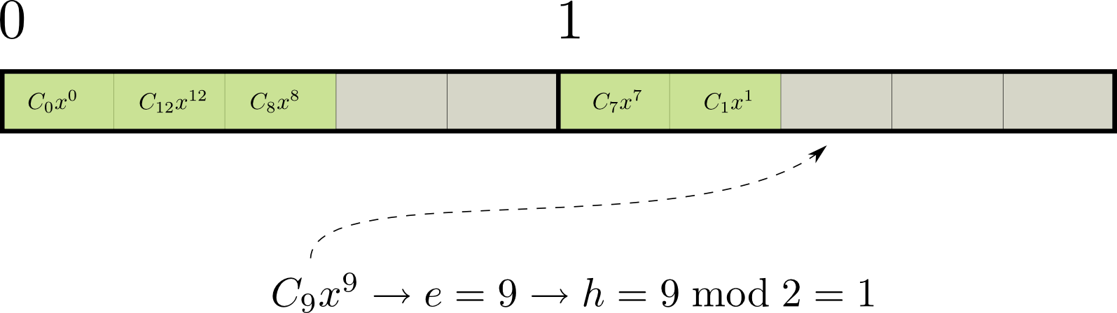
Figure 3: Insertion of monomial $C_{9}x^{9}$ into a partially-filled hash table with $n=10$, $N=2$ and $m=5$.

In order to reduce the need for resizing, an additional “overflow” bucket is allocated. When an insertion fails, the monomial is inserted into the overflow bucket, and the hash table resize is delayed until the number of monomials in the overflow bucket reaches a certain threshold $s$. The overflow bucket must also be checked whenever, during a probe of the table, a full bucket is encountered.

The cache memory optimisations introduced for the moderately sparse case can be used also for highly sparse multiplication. The only modification concerns term ordering: instead of sorting the univariate polynomial factors according to the exponents, the terms are sorted according to the exponents modulo $N$. Elementary properties of modular arithmetics ensure then that consecutive write operations happen on consecutive buckets (see Figure 4). Each time a re-hash operation takes place, the polynomial factors must be re-ordered.

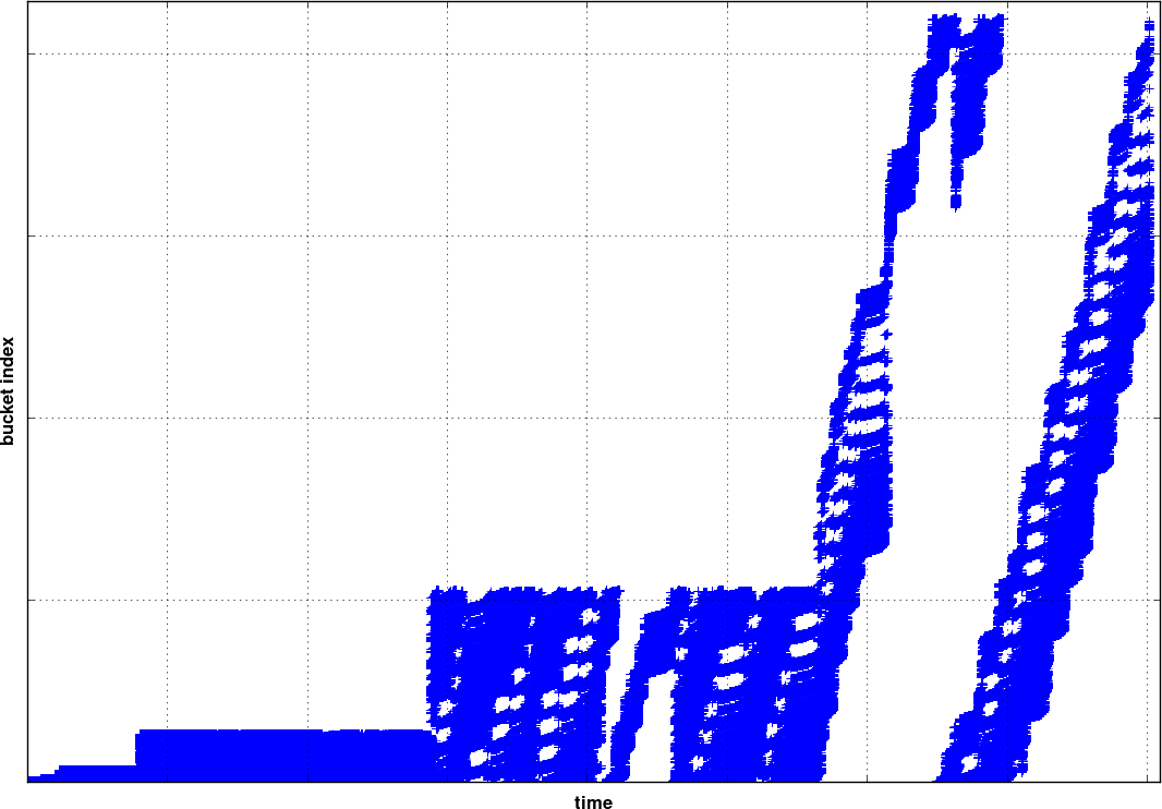
Figure 4: Typical memory access pattern for highly sparse multiplication, with cache blocking and term ordering optimisation. The $x$ axis displays the time at which the memory write is performed in the hash table, the $y$ axis displays the index of the bucket.

4 Parallelisation

The first algorithm has been parallelised for shared memory multicore architectures using multiple threads of execution. The parallelised algorithm assigns to each thread a portion of the univariate polynomial factors, and all threads concurrently write the results into the same output coefficient array. The algorithm relies on the cache memory optimisations described earlier to avoid contention. The following example explains how.

Let us suppose that the univariate polynomial factors, $P_{1}$ and $P_{2}$ have been divided into blocks. Since the monomials have been sorted according to their exponent, the $n$-th block of a polynomial will contain monomials whose exponents are bound in an interval

$$I_{n}=\left[e_{n,i},e_{n,f}\right],$$ (14)

whereas the block immediately following will feature exponents in the interval

$$I_{n+1}=\left[e_{n+1,i},e_{n+1,f}\right],$$ (15)

with

$$e_{n,f}<e_{n+1,i}.$$ (16)

From elementary interval arithmetics it follows that multiplying $P_{1}$’s block $I_{n}^{(1)}$ by $P_{2}$’s block $I_{n}^{(2)}$ will produce monomials whose exponents will be in the range

$$\left[e_{n,i}^{(1)}+e_{n,i}^{(2)},e_{n,f}^{(1)}+e_{n,f}^{(2)}\right].$$ (17)

Similarly, multiplying $P_{1}$’s block $I_{n+1}^{(1)}$ by $P_{2}$’s block $I_{n+1}^{(2)}$ will produce monomials whose exponents will be in the range

$$\left[e_{n+1,i}^{(1)}+e_{n+1,i}^{(2)},e_{n+1,f}^{(1)}+e_{n+1,f}^{(2)}\right].$$ (18)

But then, from eq. (16), the following inequality holds:

$$e_{n,f}^{(1)}+e_{n,f}^{(2)}<e_{n+1,i}^{(1)}+e_{n+1,i}^{(2)}.$$ (19)

This implies that the exponents resulting from the multiplication of $I_{n}^{(1)}$ by $I_{n}^{(2)}$ and those of $I_{n+1}^{(1)}$ by $I_{n+1}^{(2)}$ will not overlap. Hence, since the exponents encode also the memory position in the output coefficient array, this also means that performing the multiplications concurrently will not cause any contention issue, since the interested memory areas are disjoint.

The parallelised algorithm can now be explained by an example. Let us suppose, for the sake of simplicity, that there are $4$ available threads, that both univariate factors have the same length and that the chosen block size divides this length exactly, so that each factor is consituted of $n>4$ blocks. The first $4$ blocks of the first factor are assigned one per thread (so that thread $1$ is assigned block $1$, thread $2$ block $2$ and so on). Each thread starts by multiplying concurrently its block by the corresponding block in the second factor (block $1$ by block $1$, $2$ by $2$, etc.). A condition variable is used as a synchronisation barrier which all threads must reach after they have completed their block-by-block multiplications. At this point, each thread moves to the next block in the second factor, so that at this point thread $1$ is multiplying block $1$ of the first factor by block $2$ of the second factor, thread $2$ is performing $2$ by $3$ and so on. The same pattern repeats until the last block of the second factor is reached, where each thread alternately sleeps for $3$ ($=\textnormal{number of threads}-1$) iterations. These “silent” iterations are needed in order to make sure that concurrent operations are performed on consecutive blocks, as explained above. At this point the first four blocks of the first factor have been multiplied by all the blocks of the second factor; the threads acquire the next four blocks in the first factor and restart the same procedure from the top of the second factor. The sequence of block-by-block multiplications is summarised in Table 3.

This same algorithm is also applicable, albeit with some additional complications, in case of highly-sparse multiplication, where the ordering of the term according to the exponent modulo the hash table’s size ensures concurrent write on disjoint memory areas (apart from writes into the overflow bucket, which must be protected by locking). We are currently in the process of implementing this algorithm for the highly-sparse case.

$P_{1}$		$P_{2}$
$\mathbf{1}$	$\rightarrow$	$1$	$2$	$3$	$\cdots$	$n-3$	$n-2$	$n-1$	$n$	–	–	–
$\mathbf{2}$	$\rightarrow$	$2$	$3$	$4$	$\cdots$	$n-2$	$n-1$	$n$	–	–	–	$1$
$\mathbf{3}$	$\rightarrow$	$3$	$4$	$5$	$\cdots$	$n-1$	$n$	–	–	–	$1$	$2$
$\mathbf{4}$	$\rightarrow$	$4$	$5$	$6$	$\cdots$	$n$	–	–	–	$1$	$2$	$3$

Table 3: Parallel multiplication of the first four blocks of the first factor $P_{1}$ by all the blocks of the second factor $P_{2}$. The “–” symbols represent silent iterations during which no work is performed by the thread, and the vertical lines represent thread barriers. Concurrent multiplications follow column-by-column.

5 Benchmarks

The algorithms described in this paper have been implemented in C++ within a specialised algebraic manipulator for Celestial Mechanics called Piranha [4]. For comparison, we quote the results from [25], where the tested programs are SDMP [25], TRIP [13], PARI [1], Maple [24] and Magma [5]. Here we limit the comparison to SDMP, which provides the best performance according to [25] (other timings can be found in [25]). The three benchmarks we present are:

• Fateman’s benchmark [11]: calculate $f\cdot g$, where $f=\left(1+x+y+z+t\right)^{30}$ and $g=f+1$. $f$ and $g$ consist of 46376 terms. This benchmark is suitable for the first algorithm.

• ELP Poisson series multiplication: calculate $\textnormal{ELP3}^{3}\cdot\textnormal{ELP3}^{3}$, where ELP3 is the Poisson series representing the lunar distance in the main problem of the Lunar Theory ELP2000 [8]. ELP3 is a Poisson series with numerical coefficients and $\textnormal{ELP3}^{3}$ consists of 60204 terms. This benchmark is suitable for the first algorithm.

• Monagan-Pearce sparse (MP-sparse) benchmark [25]: calculate $f\cdot g$, where

  $$f=\left(1+x+y+2z^{2}+3t^{3}+5u^{5}\right)^{12}$$

  and

  $$g=\left(1+u+t+2z^{2}+3y^{3}+5x^{5}\right)^{12}.$$

  $f$ and $g$ consist of 6188 terms. This benchmark is suitable for the second algorithm.

The hardware and software configurations on which the tests were performed are displayed in Table 4. Regarding our Corei7 configuration, we have to remark here that we gained access to the machine shortly before submitting the paper and thus we were not able to conduct extensive testing. We will produce more complete benchmarks on this architecture in the future.

Short name	Hardware	Software
Core2Quad	Intel Core2 Q6600, 2.4GHz,	Linux 2.6.31.5, 64 bit,
	4 cores, 2 x 4MB L2 cache, 4GB DDR2	GCC 4.4.2, GMP 4.3.2
Core2Duo	Intel Core2 T7100, 1.8GHz,	Linux 2.6.31.2, 64-bit,
	2 cores, 2MB L2 cache, 2GB DDR2	GCC 4.4.2, GMP 4.3.1
PPC64	2 x IBM PowerPC 970, 2GHz,	Linux 2.6.32, 64-bit
	2 cores, 512KB L2 cache, 8GB DDR2	GCC 4.4.2, GMP 4.3.1
Atom	Intel Atom N270, 1.6GHz,	Linux 2.6.31.1, 32-bit,
	2 cores (Hyper-threading), 512KB L2 Cache, 1GB DDR2	GCC 4.4.2, GMP 4.3.1
Xeon	2 x Intel Xeon X5355, 2.66GHz,	Linux 2.6.28, 64-bit,
	8 cores, 2 x 4MB L2 cache, 8GB DDR2	GCC 4.3.3, GMP 4.2.4
Corei7	Intel Core i7-940, 2.93GHz, 8 cores (Hyper-threading),	OSX 10.6, 64-bit,
	4 x 256KB L2 cache, 8MB L3 cache, 4GB DDR3	Xcode 3.2, GMP 4.3.2
SDMP-Core2	Intel Core2 Q6600, 2.4GHz,	Linux 2.6.26, 64-bit,
	4 cores, 2 x 4MB L2 cache, 4GB DDR2	GCC 4.3.2, GMP 4.2.2
SDMP-Corei7	Intel Core i7-920, 2.66GHz, 4 cores	Linux 2.6.27, 64-bit,
	4 x 256KB L2 cache, 8MB L3 cache, 6GB DDR3	GCC 4.3.2, GMP 4.2.2

Table 4: Hardware and software configurations used in the benchmarks. The SDMP configurations are quoted from [25].

In the results we report both the wall clock timings and the clock cycles per monomial-by-monomial multiplication – shortened as “ccpm”. An “optimal” algorithm should be able to have a count of ccpm close to the number of clock cycles needed to multiply and add coefficients on a specific architecture, hence minimising the bookkeeping overhead and cache misses.

5.1 Sequential benchmarks

Test	Coefficient	System	Time	ccpm
Fateman	double	Core2Quad	4.29s	4.8
Fateman	double	Core2Duo	5.62s	4.6
Fateman	double	PPC64	4.96s	4.6
Fateman	double	Xeon	3.73s	4.6
Fateman	double	Atom	20.15s	15.0
Fateman	GMP mpz	Core2Quad	67.90s	75.8
Fateman	61-bit integer	SDMP-Core2	60.25s	67.2
Fateman	61-bit integer	SDMP-Corei7	70.59s	85.3
ELP	double	Core2Quad	15.62s	10.3
MP-sparse	double	Core2Quad	1.71s	107.2
MP-sparse	double	Xeon	1.59s	110.5
MP-sparse	double	Corei7	1.15s	88.0
MP-sparse	37-bit integer	SDMP-Core2	1.86s	116.6
MP-sparse	37-bit integer	SDMP-Corei7	1.56s	108.4

Table 5: Serial benchmarks. The SDMP results are quoted from [25].

The results of the benchmarks in single-thread mode are summarised in Table 5. Some considerations:

• we have performed the Fateman benchmark using both double precision and multiprecision integer coefficients (the latter implemented using the GMP library [15]). For the same test, SDMP is using 61-bit integer coefficients as input and 128-bit integer coefficients as output.

• The first algorithm is able to deliver close to optimal performance in the Fateman benchmarks. Indeed, according to [12], floating-point multiplication on most Intel CPUs has a latency of $4-5$ clock cycles. The performance degradation on the Atom might be explained by the fact the Atom is the only CPU, among those tested, that operates in-order (thus resulting in less optimisations available to the compiler).

• By comparison, Roman Pearce reported to us in a personal communication that coefficient multiplication by SDMP in the Fateman benchmark costs around 18 clock cycles.

• Performance in the ELP benchmark is also close to optimal, considering that Poisson series multiplication is slightly more complicated than polynomial multiplication.

• In the highly sparse MP-sparse benchmark, there is much more algorithmic overhead and effective cache memory usage is more difficult to achieve than in the Fateman benchmark. Our algorithm seems to benefit greatly from the high amount of cache and the DDR3 memory available on the Corei7 configuration.

5.2 Parallel benchmarks

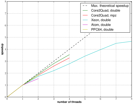
Figure 5: Speedup for the parallel Fateman benchmark on various systems. The data points for PPC64 overlap those for Core2Quad, mpz.

The speedups resulting from the parallel Fateman benchmark on various configurations are displayed in Figure 5. The speedups, calculated with respect to the sequential algorithm, are almost linear for Core2Quad, both with double precision and mpz coefficients, and also for PPC64. Also on the Atom a $\sim 1.5$ speedup is measured, despite the use of hyper-threading.

The oddball is clearly the Xeon system, which, despite exhibiting performance improvements up to all the 8 cores, features a smaller speedup with respect to the other quad-core processors benchmarked. Moreover, the results of multiple benchmark runs on this configuration resulted in timings proportionally more unstable than on the other systems. A possible explanation for this behaviour is that the machine is shared among multiple users, and, despite we made sure that no other onerous computations were going on as we performed the tests, other unrelated process (daemons, running graphical sessions, etc.) may have interfered with the benchmark. Another point of interest is that the Xeon system and the PPC64 systems are the only two configurations featuring two physically separated processors (as opposed to the other single-processor multi-core configurations). It may be possible that inter-processor communication consitutes a bottleneck for the algorithms presented here.

6 Conclusions

In this paper we have presented two algorithms for the multiplication of sparse Laurent polynomials and Poisson series on modern hardware architectures. The benchmarks performed on various hardware and software configurations suggest that these algorithms are competitive, performance-wise, with the fastest algorithm currently known and implemented in the SDMP library.

Future work will focus on the parallelisation of the highly-sparse algorithm. We also need to test the algorithms on architectures with a higher number of cores, in order to verify where the speedup limit lies; further tests are also needed to better assess the effectiveness of the algorithms on architectures with shared L3 cache, such as the Intel Core i7. Finally, we need to investigate the suboptimal speedup exhibited by the Xeon system.

7 Acknowledgements

We are very grateful to Roman Pearce for helpful discussions and useful comments.

References

- [1] PARI/GP. http://pari.math.u-bordeaux.fr, 2008.
- [2] A. Abad and J. F. San-Juan. PSPC: a Poisson Series Processor Coded in C. In K. Kurzynska, F. Barlier, P. K. Seidelmann, and I. Wyrtrzyszczak, editors, Dynamics and Astrometry of Natural and Artificial Celestial Bodies, page 383, Poznan, Poland, 1994.
- [3] I. O. Babaev, V. A. Brumberg, N. N. Vasil’Ev, T. V. Ivanova, V. I. Skripnichenko, and S. V. Tarasevich. UPP - Universal system for analytical operations with Poisson series. Astronomiya i geodeziya, 8:49–53, 1980.
- [4] F. Biscani. The Piranha algebraic manipulator. http://arxiv.org/abs/0907.2076, 2009.
- [5] W. Bosma, J. Cannon, and C. Playoust. The MAGMA algebra system I: the user language. Journal of Symbolic Computation, 24(3-4):235–265, 1997.
- [6] S. R. Bourne and J. R. Horton. The design of the Cambridge algebra system. In S. R. Petrick, editor, Symposium on Symbolic and Algebraic Manipulation - SYMSAC ’71, pages 134–143. ACM Press, 1971.
- [7] R. A. Broucke and K. Garthwaite. A programming system for analytical series expansions on a computer. Celestial Mechanics and Dynamical Astronomy, 1:271–284, June 1969.
- [8] M. Chapront-Touzé and J. Chapront. ELP2000-85: a semianalytical lunar ephemeris adequate for historical times. Astronomy and Astrophysics, 190:342–352, January 1988.
- [9] R. R. Dasenbrock. A FORTRAN-Based Program for Computerized Algebraic Manipulation. Technical Report ADA119958, Naval Research Laboratory, Washington DC (USA), September 1982.
- [10] A. Deprit. Canonical transformations depending on a small parameter. Celestial Mechanics and Dynamical Astronomy, 1:12–30, March 1969.
- [11] R. Fateman. Comparing the speed of programs for sparse polynomial multiplication. ACM SIGSAM Bulletin, 37:4–15, March 2003.
- [12] A. Fog. Lists of instruction latencies, throughputs and micro-operation breakdowns for Intel, AMD and VIA CPUs. http://www.agner.org/optimize/instruction_tables.pdf, 2009.
- [13] M. Gastineau and J. Laskar. Development of TRIP: Fast Sparse Multivariate Polynomial Multiplication Using Burst Tries, volume 3992 of Lecture Notes in Computer Science, page 446–453. Springer, Berlin (Germany), May 2006.
- [14] A. Giorgilli, U. Locatelli, and M. Sansottera. Kolmogorov and Nekhoroshev theory for the problem of three bodies. Celestial Mechanics and Dynamical Astronomy, 104:159–173, June 2009.
- [15] T. Granlund. GNU Multiple Precision Arithmetic Library. http://gmplib.org, 2009.
- [16] P. Herget and P. Musen. The calculation of literal expansions. The Astronomical Journal, 64, February 1959.
- [17] M. Herlihy, N. Shavit, and M. Tzafrir. Hopscotch Hashing, volume 5218 of Lecture Notes in Computer Science, pages 350–364. Springer Berlin Heidelberg, Berlin (Germany), 2008.
- [18] T. V. Ivanova. PSP: A new Poisson series processor. In S. Ferraz-Mello, B. Morando, and J. E. Arlot, editors, 172nd Symposium of the International Astronomical Union, page 283, Paris, France, 1996.
- [19] W. H. Jefferys. A FORTRAN-based list processor for Poisson series. Celestial Mechanics and Dynamical Astronomy, 2:474–480, December 1970.
- [20] W. H. Jefferys. A precompiler for the formula manipulation system TRIGMAN. Celestial Mechanics and Dynamical Astronomy, 6:117–124, August 1972.
- [21] D. E. Knuth. The Art of Computer Programming, volume 3: Sorting and Searching. Addison-Wesley, second edition, 1998.
- [22] L. Kronecker. Grundzüge einer arithmetischen Theorie der algebraischen Grössen. Journal Für die reine und angewandte Mathematik, 92:1–122, 1882.
- [23] E. D. Kuznetsov and K. V. Kholshevnikov. Expansion of the Hamiltonian of the Two-Planetary Problem into the Poisson Series in All Elements: Application of the Poisson Series Processor. Solar System Research, 38:147–154, March 2004.
- [24] M. B. Monagan, K. Geddes, K. Heal, G. Labahn, S. Vorkoetter, J. McCarron, and P. DeMarco. Maple 13 Introductory Programming Guide. Maplesoft, 2009.
- [25] M. B. Monagan and R. Pearce. Parallel sparse polynomial multiplication using heaps. In J. Johnson, H. Park, and E. Kaltofen, editors, 2009 International symposium on Symbolic and algebraic computation - ISSAC ’09, pages 263–270, Seoul (Republic of Korea), 2009. ACM Press.
- [26] A. Morbidelli. Modern Celestial Mechanics: aspects of Solar System dynamics. Number 5 in Advances in Astronomy and Astrophysics. Taylor & Francis, London, first edition, 2002.
- [27] R. Pagh and F. F. Rodler. Cuckoo hashing. Journal of Algorithms, 51:122–144, May 2004.
- [28] D. L. Richardson. PARSEC: An interactive Poisson series processor for personal computing systems. Celestial Mechanics and Dynamical Astronomy, 45:267–274, March 1988.
- [29] A. Rom. Mechanized Algebraic Operations (MAO). Celestial Mechanics, 1:301–319, September 1970.
- [30] J. F. San-Juan and A. Abad. Algebraic and symbolic manipulation of Poisson series. Journal of Symbolic Computation, 32:565–572, September 2001.