Spin density matrices for nuclear density functionals with parity violations

Abstract

The spin density matrix (SDM) used in atomic and molecular physics is revisited for nuclear physics, in the context of the radial density functional theory. The vector part of the SDM defines a “hedgehog” situation, which exists only if nuclear states contain some amount of parity violation.

PACS: 21.10.-k, 21.10.Dr, 21.10.Hw, 21.60.-n

1 Introduction

The subject of density functionals (DFs) in nuclear physics [1, 2] is presently receiving intense attention. One of its difficulties is the handling of interactions that depend on spins. While there is a priori no theorem preventing a theory with simple densities from accommodating the influence of spin dependent forces, it is likely that a generalization of density profiles to “spin density” ones should, in practice, make the construction of a DF easier. The purpose of this paper is see whether one can adapt to nuclear physics the same concept [3, 4] as that used for many years in atomic and molecular physics.

Given the creation and annihilation operators, $a_{\vec{r}\sigma}^{\dagger}$ and $a_{\vec{r}\sigma},$ respectively, of a nucleon with spin $\sigma=\pm\frac{1}{2}$ at position $\vec{r},$ and given a density operator ${\cal D}$ in many-body space, the SDM, $\bar{\rho}(\vec{r}),$ is defined by its matrix elements,

$$\rho_{\sigma\sigma^{\prime}}(\vec{r})={\rm Tr}\,a_{\vec{r}\,\sigma}^{\dagger}\,a_{\vec{r}\,\sigma^{\prime}}\,{\cal D}\,.$$ (1)

In the following, we shall take advantage of the recent proof [5], based upon the rotational invariance of the nuclear Hamiltonian, that the nuclear DF is a scalar, namely a radial density functional (RDF); accordingly, it is understood in the following, unless explicitly stated otherwise, that the density operator, ${\cal D},$ in many-body space, is a scalar under rotations. Since practical calculations for a DF can eventually result in Kohn-Sham (KS) potentials [6], the approach described by the present paper, with its explicit treatment of spin, might give indications for the spin-orbit term in KS equations.

The basic formalism for the SDM is explained in Sec. 2. A mandatory generalisation of the formalism is explained in Sec. 3. An illustrative example is provided in Sec. 4. We conclude in Sec. 5.

2 Basic formalism

We first relate the local creation and annihilation operators to those of an $\ell s$ shell model,

$$a_{\vec{r}\,\sigma}^{\dagger}=\sum_{n\ell m}\varphi_{n\ell}(r)\,Y_{\ell m}^{*}(\hat{r})\,a_{n\ell m\sigma}^{\dagger}\,,\ \ \ \ a_{\vec{r}\,\sigma^{\prime}}=\sum_{n^{\prime}\ell^{\prime}m^{\prime}}\varphi_{n^{\prime}\ell^{\prime}}(r)\,Y_{\ell^{\prime}m^{\prime}}(\hat{r})\,a_{n^{\prime}\ell^{\prime}m^{\prime}\sigma^{\prime}}\,.$$ (2)

Here the wave functions, $\varphi_{n\ell}(r)\,Y_{\ell m}(\hat{r}),$ represent the orbitals created by the operators $a_{n\ell m}^{\dagger},$ with real radial form factors $\varphi_{n\ell}(r).$ The summation, $\sum_{n\ell m},$ runs over a complete basis of orbitals, assumed to be discrete for the sake of simplicity. A generalization with continuum orbitals brings no difficulty except for slightly less simple notations. Isospin labels are understood.

We then rearrange the products, $a_{\vec{r}\sigma}^{\dagger}a_{\vec{r}\sigma^{\prime}},$ into their scalar and vector parts in spin space with the usual Clebsch-Gordan coefficients,

$$A_{\vec{r}SM_{S}}=\sum_{\sigma\sigma^{\prime}}(-)^{\frac{1}{2}-\sigma^{\prime}}\langle\frac{1}{2}\,\sigma\,\frac{1}{2}\,-\sigma^{\prime}|S\,M_{S}\rangle\,a_{\vec{r}\sigma}^{\dagger}a_{\vec{r}\sigma^{\prime}},$$ (3)

This gives, after inserting Eqs. (2),

$$A_{\vec{r}SM_{S}}=\sum_{\ell m\ell^{\prime}m^{\prime}}Y_{\ell m}^{*}(\hat{r})\,Y_{\ell^{\prime}m^{\prime}}(\hat{r})\,B_{\ell m\ell^{\prime}m^{\prime}SM_{S}}(r)\,,$$ (4)

with

$$B_{\ell m\ell^{\prime}m^{\prime}SM_{S}}(r)=$$

$$\sum_{nn^{\prime}\sigma\sigma^{\prime}}\varphi_{n\ell}(r)\,\varphi_{n^{\prime}\ell^{\prime}}(r)\,(-)^{\frac{1}{2}-\sigma^{\prime}}\langle\frac{1}{2}\,\sigma\,\frac{1}{2}\,-\sigma^{\prime}|S\,M_{S}\rangle\,a_{n\ell m\sigma}^{\dagger}a_{n^{\prime}\ell^{\prime}m^{\prime}\sigma^{\prime}}\,.$$ (5)

Next we recouple the orbital momenta carried by the operators $B_{\ell m\ell^{\prime}m^{\prime}SM_{S}}\,,$

$$C_{\ell\ell^{\prime}LMSM_{S}}(r)=\sum_{m_{1}m_{2}}(-)^{\ell^{\prime}-m_{2}}\,\langle\ell\,m_{1}\,\ell^{\prime}\,-m_{2}|L\,M\rangle\,B_{\ell m_{1}\ell^{\prime}m_{2}SM_{S}}(r)\,,$$ (6)

so that

$$A_{\vec{r}SM_{S}}=\sum_{\ell m\ell^{\prime}m^{\prime}}Y_{\ell m}^{*}(\hat{r})\,Y_{\ell^{\prime}m^{\prime}}(\hat{r})\,(-)^{\ell^{\prime}-m^{\prime}}\,\sum_{LM}\langle\ell\,m\,\ell^{\prime}\,-m^{\prime}|LM\rangle\,C_{\ell\ell^{\prime}LMSM_{S}}(r)\,.$$ (7)

Upon taking advantage of the relations i) between spherical harmonics,

$$Y_{\ell m}(\hat{r})\,Y_{\ell^{\prime}m^{\prime}}^{*}(\hat{r}) = (-)^{m^{\prime}}\,\sum_{\lambda\mu}\sqrt{\frac{(2\ell+1)\,(2\ell^{\prime}+1)\,(2\lambda+1)}{4\pi}}\ \times$$ (8)

$$\left(\matrix{\ell&\ell^{\prime}&\lambda\cr 0&0&0}\right)\,\left(\matrix{\ell&\ell^{\prime}&\lambda\cr m&-m^{\prime}&\mu}\right)Y_{\lambda\mu}^{*}(\hat{r})\,,$$

and ii) between Wigner $3j$-coefficients and Clebsch-Gordan ones,

$$\langle l\,m\,l^{\prime}\,-m^{\prime}|L\,M\rangle=(-)^{\ell-\ell^{\prime}+M}\,\sqrt{2L+1}\,\left(\matrix{\ell&\ell^{\prime}&L\cr m&-m^{\prime}&-M}\right)\,,$$ (9)

the orthogonality between Wigner $3j$-coefficients,

$$\sum_{mm^{\prime}}(2L+1)\,\left(\matrix{\ell&\ell^{\prime}&L\cr m&-m^{\prime}&-M}\right)\,\left(\matrix{\ell&\ell^{\prime}&\lambda\cr m&-m^{\prime}&\mu}\right)=\delta_{L\lambda}\,\delta_{-M\,\mu}\,,$$ (10)

simplifies Eq. (7) into,

$$A_{\vec{r}SM_{S}} = \sum_{\ell\ell^{\prime}LM}(-)^{L-M}\,Y_{L-M}(\hat{r})\times$$ (11)

$$(-)^{\ell^{\prime}}\,\sqrt{\frac{(2\ell+1)(2\ell^{\prime}+1)}{4\pi}}\,\left(\matrix{\ell&\ell^{\prime}&L\cr 0&0&0}\right)\,C_{\ell\ell^{\prime}LMSM_{S}}(r)\,.$$

In Eq. (11), we used the facts that all numbers, $\ell,\ell^{\prime},L,M,$ are integers and that the $3j$-coefficient, $\left(\matrix{\ell&\ell^{\prime}&L\cr 0&0&0}\right),$ vanishes unless $\ell+\ell^{\prime}+L$ is even.

Finally, a recoupling of total orbital momentum and total spin yields,

$$D_{LSJ\mu}(r)=\sum_{MM_{S}}\langle LMSM_{S}|J\mu\rangle\ \times$$

$$\left[\sum_{\ell\ell^{\prime}}\,(-)^{\ell^{\prime}}\sqrt{\frac{(2\ell+1)(2\ell^{\prime}+1)}{4\pi}}\left(\matrix{\ell&\ell^{\prime}&L\cr 0&0&0}\right)C_{\ell\ell^{\prime}LMSM_{S}}(r)\right],$$ (12)

so that,

$$\sum_{\ell\ell^{\prime}}\,(-)^{\ell^{\prime}}\,\sqrt{\frac{(2\ell+1)(2\ell^{\prime}+1)}{4\pi}}\,\left(\matrix{\ell&\ell^{\prime}&L\cr 0&0&0}\right)\,C_{\ell\ell^{\prime}LMSM_{S}}(r)=$$

$$\sum_{J\mu}\langle LMSM_{S}|J\mu\rangle\,D_{LSJ\mu}(r)\,.$$ (13)

In terms of $D_{LSJ\mu}(r),$ the scalar or vector operators for the SDM now read

$$A_{\vec{r}SM_{S}}=\sum_{LM}(-)^{L}\,Y_{LM}^{*}(\hat{r})\sum_{J\mu}\langle L\,M\,S\,M_{S}|J\mu\rangle\,D_{LSJ\mu}(r)\,.$$ (14)

With scalar density matrices ${\cal D}$ in many-body space, there will be vanishing traces, ${\rm Tr}\,D_{LSJ\mu}(r)\,{\cal D},$ unless $J=\mu=0.$ In this case, the corresponding Clebsch-Gordan coefficient becomes,

$$\langle L\,M\,S\,M_{S}|0\,0\rangle=\delta_{LS}\ \delta_{M\,-M_{S}}\ \frac{(-)^{S+M_{S}}}{\sqrt{2S+1}}\,,$$ (15)

so that the SDM scalar or vector elements reduce to,

$${\rm Tr}\,A_{\vec{r}SM_{S}}\,{\cal D}=\frac{(-)^{M_{S}}\,Y_{S\,-M_{S}}^{*}(\hat{r})}{\sqrt{2S+1}}\,{\rm Tr}\,D_{SS00}(r)\,{\cal D}=\frac{Y_{SM_{S}}(\hat{r})}{\sqrt{2S+1}}\,{\rm Tr}\,D_{SS00}(r)\,{\cal D}\,.$$ (16)

3 Generalization

Two very different spin profiles emerge from the study made in Sec. 2. For the first of them, namely, for $S=0,$ the result is simple, since, necessarily in this case, $\ell$ and $\ell^{\prime}$ are equal,

$$D_{0000}(r)=\frac{1}{\sqrt{8\pi}}\,\sum_{nn^{\prime}\ell m\sigma}\varphi_{n\ell}(r)\,\varphi_{n^{\prime}\ell}(r)\,a_{n\ell m\sigma}^{\dagger}\,a_{n^{\prime}\ell m\sigma}\,.$$ (17)

For the second profile, i.e., for $S=1,$ spherical symmetry is ensured by the fact that all three spherical harmonics are multiplied by the same, radial form factor, which we denote $\rho_{hh}(r)$ in the following; we have a ‘hedgehog” situation. Here we mean hedgehog-like in the sense that the vector spin field has only a radial dependency. It must be noticed, however, that only those pairs of particle orbital momenta $\{\ell,\ell^{\prime}\},$ where $|\ell-\ell^{\prime}|\leq 1,$ can couple to $L=1.$ If $\ell=\ell^{\prime},$ the $3j$-coefficient, $\left(\matrix{\ell&\ell^{\prime}&L\cr 0&0&0}\right),$ vanishes identically, since $\ell+\ell^{\prime}+1$ becomes odd. Conversely, if $\ell-\ell^{\prime}=\pm 1,$ the corresponding products of operators, $a_{n\ell m}^{\dagger}a_{n^{\prime}\ell^{\prime}m^{\prime}},$ have an odd parity. Since parity violations in nuclear states are most often too tiny to be observable, the density operators ${\cal D}$ of interest always have an even parity. Therefore, if the traces, ${\rm Tr}\,C_{\ell\,\ell\pm 1\,1\,-M_{S}\,1\,M_{S}}(r)\,{\cal D},$ do not vanish completely, then they will detect parity violations in ${\cal D}.$ A basic RDF, that uses $D_{0000}$ only, has no easy signature for parity violations. It is the occurrence of a tiny, but non-vanishing profile from $D_{1100}$ that allows a more elaborate RDF theory to explicitly accommodate parity violations.

For the sake of completeness, we show in Eq. (18) this “hedgehog” operator, $D_{hh}(r)\equiv D_{1100}/\sqrt{3},$ the trace of which with ${\cal D}$ is the coefficient of $Y_{1M_{S}}(\hat{r})$ in Eq. (16). It reads, upon taking advantage of Eqs. (5), (6), (12) and (16),

$$D_{hh}(r) = \frac{1}{3\sqrt{4\pi}}\,\sum_{nn^{\prime}\ell m\ell^{\prime}m^{\prime}\sigma\sigma^{\prime}M_{S}}\,\varphi_{n\ell}(r)\,\varphi_{n^{\prime}\ell^{\prime}}(r)\,(-)^{1+M_{S}-m^{\prime}+\frac{1}{2}-\sigma^{\prime}}\ \times$$ (18)

$$\sqrt{(2\ell+1)(2\ell^{\prime}+1)}\,\left(\matrix{\ell&\ell^{\prime}&1\cr 0&0&0}\right)\,\langle\ell\,m\,\ell^{\prime}\,-m^{\prime}|1\,-M_{S}\rangle\,\ \times$$

$$\langle\frac{1}{2}\,\sigma\,\frac{1}{2}\,-\sigma^{\prime}|1\,M_{S}\rangle\,a_{n\ell m\sigma}^{\dagger}\,a_{n^{\prime}\ell^{\prime}m^{\prime}\sigma^{\prime}}\,.$$

A natural way to enlarge the theory to cases where the $S=1$ form factor is not tiny consists in embedding the nucleus in an external field, $H_{1},$ that simultaneously breaks the rotational symmetry and the parity. To avoid loosing the advantage of an RDF, i.e., the reduction of three-dimensional calculations to one-dimensional ones, the symmetry breaking can be chosen as a minimal one, in the following way. Let $H_{1}$ be a negative parity operator, bounded from below, that transforms as a vector under rotations. There is no need to assume that $H_{1}$ is only made of local fields, $H_{1}=\sum_{i}h_{1}(\vec{r}_{i},\sigma_{i}),$ where $\vec{r}_{i}$ and $\sigma_{i}$ denote the position and spin of the $i$th nucleon; any complicated $H_{1}$ is allowed for the argument to come. What counts is that the extended Hamiltonian, $H^{\prime}=H+H_{1},$ which is bounded from below, now contains, besides the basic scalar and positive parity $H,$ a vector and negative parity component $H_{1}.$ Then we use the “constrained search” definition [7] of a DF,

$$F[\bar{\rho}]={\rm Inf}_{{\cal D}\rightarrow\bar{\rho}}\,{\rm Tr}\,H^{\prime}\,{\cal D},$$ (19)

where now ${\cal D}$ is generalized into an arbitrary density operator, without symmetry properties. Here the symbol, ${\cal D}\rightarrow\bar{\rho},$ means that the minimization of the energy is performed over subsets in the ${\cal D}$ space that show a given spin density matrix $\bar{\rho}.$ Then the same argument, as that used in [5], to restrict ${\cal D}$ to be a rotation scalar, can be extended to restrict ${\cal D}$ to be a mixture ${\cal D}_{01}$ of a scalar and a vector. Next one can take advantage of Eq. (14) and derive $F[\bar{\rho}]$ from those few and radial profile operators, $D_{LSJ\mu}(r)$, where the conditions, $S=0,1$ and $J=0,1$ give limits to $L$ via the usual triangular rules.

To conclude this Sec., we note that a spin density DF is usually not very useful for an isolated nucleus, but becomes legitimate for a non-isolated one.

4 Toy model for an illustrative example

Consider a fictitious ¹⁶O nucleus made of a full $0s$ shell and an almost full $0p$ shell and driven by a harmonic oscillator Hamiltonian,

$$H_{0}=\sum_{nlm\sigma\tau}\left(2n+\ell+\frac{3}{2}\right)a_{n\ell m\sigma\tau}^{\dagger}\,a_{n\ell m\sigma\tau}=\sum_{nlj\mu\tau}\left(2n+\ell+\frac{3}{2}\right)b_{n\ell j\mu\tau}^{\dagger}\,b_{n\ell j\mu\tau}\,.$$

Here, temporarily, the isospin label, $\tau=\pm\frac{1}{2},$ is explicit. The relation between $\ell s$ and $jj$ creation operators (and, similarly, for annihilation ones) in this toy model reads,

$$b_{n\ell j\mu\tau}^{\dagger}=\sum_{m\sigma}\langle\ell m\frac{1}{2}\sigma|j\mu\rangle\,a_{n\ell m\sigma\tau}^{\dagger}\,,\ \ a_{n\ell m\sigma\tau}^{\dagger}=\sum_{j\mu}\langle\ell m\frac{1}{2}\sigma|j\mu\rangle\,b_{n\ell j\mu\tau}^{\dagger}\,.$$ (20)

A Slater determinant, $|\phi\rangle,$ will describe this nucleus for our model. Assume that a perturbation of the harmonic oscillator slightly mixes the $0p_{\frac{1}{2}}$ orbitals with the $1s_{\frac{1}{2}}$ orbitals. The mixtures read,

$$\beta_{\,j=\frac{1}{2},\mu,\tau}^{\dagger}=\cos\varepsilon\ b_{\,0p\frac{1}{2},\mu,\tau}^{\dagger}+\sin\varepsilon\ b_{\,1s\frac{1}{2},\mu,\tau}^{\dagger}\,.$$ (21)

We keep intact a core, made of the $0s$ and $0p\frac{3}{2}$ orbitals. The $16$-body operator, ${\cal D}=|\phi\rangle\langle\phi|,$ is still a scalar under rotations, but it has now a negative parity component at first order in $\varepsilon.$ Such a state, and similar density matrices, would justify the use of a “spin RDF”, with two profiles.

Let $|0\rangle$ denote the fully closed $0s$ and $0p$ shells. At first order in $\varepsilon,$ the wave function under consideration is, $|\phi\rangle=|0\rangle+\varepsilon\sum_{\tau}|\tau\rangle,$ with

$$|\tau\rangle=\left(b_{\,1s\frac{1}{2},\frac{1}{2},\tau}^{\dagger}\,b_{\,0p\frac{1}{2},\frac{1}{2},\tau}+b_{\,1s\frac{1}{2},-\frac{1}{2},\tau}^{\dagger}\,b_{\,0p\frac{1}{2},-\frac{1}{2},\tau}\right)|0\rangle.$$ (22)

Protons and neutrons will give equal matrix elements; hence, within an inessential factor of 2, isospin labels and summations can again be omitted. Notice also, incidentally, that the particle-hole states $|\tau\rangle,$ shown in Eq. (22), do not represent center-of-mass spurious shifts; the latter induce dipoles, not monopoles, in the one-particle-one-hole space.

In the $jj$ representation, we obtain for the $S=0$ case

$$D_{0000}(r)=\frac{1}{\sqrt{8\pi}}\,\sum_{nn^{\prime}\ell j}\varphi_{n\ell}(r)\,\varphi_{n^{\prime}\ell}(r)\,\sum_{\mu}b_{n\ell j\mu}^{\dagger}\,b_{n^{\prime}\ell j\mu}\,,$$ (23)

and the scalar profile, ${\rm Tr}D_{0000}|\phi\rangle\langle\phi|,$ has a vanishing contribution from the first-order matrix elements, $\langle 0|D_{0000}|\tau\rangle=\langle\tau|D_{0000}|0\rangle=0,$ because of the restriction to equal values of $\ell$. The zeroth-order profile from the $0s$- and $0p$-shells, respectively, is obviously

$$D_{0000}(r)\propto\varphi_{00}^{2}(r)+3\,\varphi_{01}^{2}(r)=\left(2\pi^{-\frac{1}{4}}\,e^{-\frac{1}{2}r^{2}}\right)^{2}+3\left(2^{\frac{3}{2}}3^{-\frac{1}{2}}\pi^{-\frac{1}{4}}\,r\,e^{-\frac{1}{2}r^{2}}\right)^{2},$$ (24)

with an inessential coefficient, $\sqrt{2/\pi},$ omitted for simplicity.

Again for the $jj$ representation, we find for the $S=1$ (hedgehog) case,

$$D_{hh}(r) = \frac{1}{3\sqrt{4\pi}}\,\sum_{nn^{\prime}\ell\ell^{\prime}jj^{\prime}\mu\mu^{\prime}mm^{\prime}\sigma\sigma^{\prime}M_{S}}\,\varphi_{n\ell}(r)\,\varphi_{n^{\prime}\ell^{\prime}}(r)\,(-)^{1+M_{S}-m^{\prime}+\frac{1}{2}-\sigma^{\prime}}\ \times$$ (25)

$$\sqrt{(2\ell+1)(2\ell^{\prime}+1)}\,\left(\matrix{\ell&\ell^{\prime}&1\cr 0&0&0}\right)\,\langle\ell\,m\,\ell^{\prime}\,-m^{\prime}|1\,-M_{S}\rangle\,\ \times$$

$$\langle\frac{1}{2}\,\sigma\,\frac{1}{2}\,-\sigma^{\prime}|1\,M_{S}\rangle\,\langle\ell m\frac{1}{2}\sigma|j\mu\rangle\,b_{n\ell j\mu}^{\dagger}\,\langle\ell^{\prime}m^{\prime}\frac{1}{2}\sigma^{\prime}|j^{\prime}\mu^{\prime}\rangle\,b_{n^{\prime}\ell^{\prime}j^{\prime}\mu^{\prime}}\,,$$

which reduces into,

$$D_{hh}(r) = \frac{1}{\sqrt{4\pi}}\sum_{nn^{\prime}\ell\ell^{\prime}j}(-)^{j-\frac{1}{2}}\,\sqrt{(2\ell+1)(2\ell^{\prime}+1)}\,\varphi_{n\ell}(r)\,\varphi_{n^{\prime}\ell^{\prime}}(r)$$ (26)

$$\left(\matrix{\ell&\ell^{\prime}&1\cr 0&0&0}\right)\,\left\{\matrix{l&l^{\prime}&1\cr\frac{1}{2}&\frac{1}{2}&j}\right\}\,\sum_{\mu}b_{n\ell j\mu}^{\dagger}\,b_{n^{\prime}\ell^{\prime}j\mu}\,,$$

where $\{\ \}$ is a Wigner $6j$ symbol. The equalities, $j=j^{\prime}$ and $\mu=\mu^{\prime},$ reflect the fact that the $LS$ coupling used in the previous section, Sec. 3, boils down to total spin $J=0,$ as demanded by the scalar nature of the many-body density operator ${\cal D}.$ Accordingly, in a $jj$ scheme, both the particle and the hole total spin labels must be equal.

The zeroth-order matrix element in $\varepsilon$ that results from Eqs. (22) and (26), $\langle 0|D_{hh}|0\rangle,$ trivially vanishes. Upon a simple inspection of the first-order matrix elements, $\langle 0|\,b_{n\ell j\mu}^{\dagger}\,b_{n^{\prime}\ell^{\prime}j\mu}\,b_{\,1s\frac{1}{2}\nu}^{\dagger}\,b_{\,0p\frac{1}{2}\nu}\,|0\rangle,$ it is seen that the only non-vanishing contributions come from the cases, $\{n\ell j\mu\}=0p_{\frac{1}{2}}\nu$ and $\{n^{\prime}\ell^{\prime}j\mu\}=1s_{\frac{1}{2}}\nu$, because of the restrictions on the values of $\ell$ and $\ell^{\prime}$. Here $\nu$ denotes the magnetic label of both the particle and the hole in Eq. (22).The two values of $\nu$ in $|\tau\rangle$ give the same contribution, similarly to the two isospin components. With a global factor, $4\,\sqrt{3/\pi}\,\left(\matrix{1&0&1\cr 0&0&0}\right)\,\left\{\matrix{1&0&1\cr\frac{1}{2}&\frac{1}{2}&\frac{1}{2}}\right\},$ omitted, the $S=1$ form factor for the toy model reads,

$$D_{hh}(r)\propto\varphi_{01}(r)\,\varphi_{10}(r)=\pi^{-\frac{1}{2}}\,\left(2^{\frac{3}{2}}3^{-\frac{1}{2}}\,r\,e^{-\frac{r^{2}}{2}}\right)\,\left[6^{\frac{1}{2}}\left(1-\frac{2}{3}r^{2}\right)\,e^{-\frac{r^{2}}{2}}\right].$$ (27)

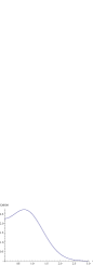
Figure 1: Scalar profile of the toy model

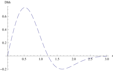
Figure 2: Vector profile of the toy model

Figures 1 and 2 show these scalar and vector profiles, respectively, in arbitrary units to avoid unessential global coefficients and because we prefer to compare shapes. There is no need to stress how different their shapes are.

5 Discussion

We set out to investigate the possible role of the spin density matrix in the construction of the density functional for nuclei. Such spin densities have played an important role in atomic and molecular physics. However, the severe constraints of rotational invariance and parity for nuclei led to the result that the vector part of the spin density essentially vanishes in a nuclear DF that properly takes into account such symmetries, namely, in an RDF. Thus, there is no way, in this approach, to explicitly describe spin properties in a nuclear RDF. On the other hand, the vector part becomes a signature of parity violation allowed in the RDF theory. We were able to legitimize the use of a spin density RDF, at the cost of introducing an external perturbation that has negative parity and transforms as a vector. Future studies are needed to understand the role of the spin-density-matrix formalism, when symmetries are broken by external forces.

Acknowledgments: B.R.B.and B.G.G. thank B.K. Jennings and T. Papenbrock for stimulating and helpful discussions. B.R.B. and B.G.G. also thank TRIUMF, Vancouver, B. C., Canada, for its hospitality, where part of this work was done. The Natural Science and Engineering Research Council of Canada is thanked for financial support. TRIUMF receives federal funding via a contribution agreement through the National Research Council of Canada. B.R.B. also thanks Institut de Physique Théorique, CEA Saclay, France, for its hospitality, where part of this work was carried out, and acknowledges partial support by NSF grants PHY-0555396 and PHY-0854912 and by Institut de Physique Théorique, CEA Saclay.

References

• [1] UNEDF SciDAC Collaboration, www.unedf.org/
• [2] J. E. Drut, R. J. Furnstahl, and L. Platter, Prog. Part. Nucl. Phys. 64, 120 (2010) and references cited therein; arXiv:nucl-th:0906.1463 (2009),
• [3] O. Gunnarson and B. J. Lundqvist, Phys. Rev. B 13, 4274 (1976).
• [4] A. Görling, Phys. Rev. A 47, 2783 (1993).
• [5] B.G. Giraud, Phys. Rev. C 78, 014307 (2008).
• [6] W. Kohn and L. J. Sham, Phys. Rev. 140, A1133 (1965). .
• [7] M. Levy, PNAS 76 6062 (1979); E.H. Lieb, Int. J. Quant. Chem. 24, 243 (1983).