Flux periodicities in loops and junctions with $d$-wave superconductors

Abstract

The magnetic flux periodicity in superconducting loops is reviewed. Whereas quantization of the magnetic flux with $hc/2e$ prevails in sufficiently thick loops with current free interior, the supercurrent in narrow loops is either $hc/2e$ or $hc/e$ periodic with the external magnetic flux. The periodicity depends on the properties of the condensate state, in particular on the Doppler shift of the energy spectrum. For an $s$-wave superconductor in a loop with diameter larger than the coherence length $\xi_{0}$, the Doppler shift is small with respect to the energy gap, and the $hc/2e$ periodic behavior of its flux dependent thermodynamic properties is maintained. However, for smaller $s$-wave loops and, more prominently, narrow $d$-wave loops of any diameter $R$, the Doppler shift has a strong effect on the supercurrent carrying state; as a consequence, the fundamental flux periodicity is in fact $hc/e$. It is shown analytically and numerically that the $hc/e$ periodic component in the supercurrent decays only algebraically as $1/R$ for large $d$-wave loops. For nodal superconductors the discrete nature of the eigenergies close to the Fermi energy has to be respected in the evaluation of the Doppler shift. Furthermore, we investigate, whether the Doppler shift modifies the supercurrent through Josephson junctions with $d$-wave superconductors. For transparent junctions, the Josephson current behaves similar to the persistent supercurrent in a loop. These distinct physical phenomena can be compared, if the magnetic flux $\Phi=\phi\cdot hc/e$ is identified with the phase variation of the order parameter $\delta\varphi$ through $2\pi\phi=\delta\varphi/2$. Correspondingly, the Josephson current can display a $4\pi$ periodicity in $\delta\varphi$, if the Doppler shift is sufficiently strong which is true for transparent junctions of $d$-wave superconductors. Moreover, a $4\pi$ periodicity is also valid for the current-flux relation of field-threaded junctions. In the tunneling regime the microscopic theory reproduces the results of the Ginzburg-Landau description for sufficiently wide Josephson junctions.

I Introduction

The quantum mechanical wave function $\psi$ of particles moving in a multiply connected geometry has to be a unique function of the spatial coordinate. This condition leads to a discrete energy spectrum, because the phase difference of the wave function accumulated on a closed path has to be $2\pi k$, where the integer $k$ serves as a quantum number of the wave function. For a circular geometry, this phase winding number $k$ represents the angular momentum $\hbar k$ of the particles.

In the presence of a magnetic field ${\bf B}({\bf r})=\nabla\times{\bf A}({\bf r})$, an additional term adds to the phase of the wave function: $\psi^{\prime}=\psi\exp(-{\rm i}\,2\pi(e/hc)\int_{{\bf r}_{0}}^{\bf r}{\rm d}{\bf r}^{\prime}\cdot{\bf A}({\bf r}^{\prime}))$, where ${\bf A}({\bf r})$ is the vector potential, $e$ the charge of the electron, $c$ the velocity of light, $h$ is Planck’s constant, and ${\bf r}_{0}$ an arbitrary space point within the system. The gauge transformed wave function $\psi^{\prime}$ satisfies the Schrödinger equation with the vector potential ${\bf A}$ eliminated from the kinetic energy term. The new condition is that $\psi^{\prime}$ acquires the phase factor $\exp(-i2\pi(e/hc)\Phi)$ for a path $C$ enclosing the magnetic flux $\Phi=\int_{C}{\rm d}{\bf r}\cdot{\bf A}({\bf r})$. This leads to a total phase difference of $2\pi(k-e\Phi/hc)$ on the closed path $C$. Because physical quantities are obtained by a thermal average over all possible $k$, they are periodic in $\Phi$ with the fundamental period

$$\Phi_{0}=hc/e,$$ (1)

which is the flux quantum in the normal state. In particular, the persistent current $J(\Phi)$ induced by the magnetic flux vanishes whenever $\Phi/\Phi_{0}$ is an integer.

The effect described above is present in any system with sufficient phase coherence, and best known from the periodic resistance modulations of a microscopic metallic loop, predicted first by Ehrenberg and Siday in 1948 ehrenberg and in 1959 by Aharonov and Bohm AB . Already ten years earlier, London predicted the manifestation of a similar effect in superconducting loops, where the phase coherence is naturally macroscopic London : the magnetic flux threading the loop is quantized in multiples of $\Phi_{0}$, because the interior of a superconductor has to be current free. London did not know about the existence of $\Phi_{0}/2$ flux quanta in superconductors, but he already speculated that the supercurrent might be carried by pairs of electrons with charge $2e$ and that the superconducting flux quantum and hence the flux periodicity of the supercurrent is rather $\Phi_{0}/2$. This point of view became generally accepted after the ‘Theory of Superconductivity’ by Bardeen, Cooper, and Schrieffer (BCS) was published in 1957 bcs . Direct measurements of magnetic flux quanta $\Phi_{0}/2$ trapped in superconducting rings followed in 1961 by Doll and Näbauer Doll and by Deaver and Fairbank Deaver , corroborated later by the detection of $\Phi_{0}/2$ flux lines in the vortex phase of type II superconductors Abrikosov ; Essmann .

For thin superconducting loops with walls thinner than the penetration depth $\lambda$, finite currents are flowing throughout the entire superconductor. The magnetic flux is consequently not quantized, but London introduced instead the quantity $\Phi^{\prime}=\Phi+\Lambda/c\oint{\rm d}{\bf r}\cdot{\bf J}({\bf r})$, the quantized “fluxoid”. The flux $\Phi$ is the total flux threading the loop, which already includes the current induced flux. $\Lambda$ is a phenomenological constant parametrizing the strength of the current response of the superconductor to the applied magnetic field; $\Lambda$ is related to the penetration depth via $\Lambda=4\pi\lambda^{2}/c^{2}$ through the London equation London . Thin superconducting loops therefore react periodically to the continuous variable $\Phi$.

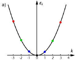
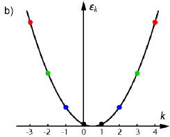
Figure 1: Scheme of the pairing of angular-momentum eigenstates in a one dimensional metal loop for (a) $\Phi=0$ and (b) $\Phi=\Phi_{0}/2$, as used by Schrieffer in schrieffer to illustrate the origin of the $\Phi_{0}/2$ periodicity in superconductors. Paired are states with equal energy, which leads to pairs with a center-of-mass angular momentum $q=0$ in (a) and $q=1$ in (b) in units of $\hbar$.

It is tempting to relate the $\Phi_{0}/2$ flux periodicity of superconducting loops to the charge $2e$ of the Cooper pairs onsager:61 which carry the supercurrent, but the pairing of electrons alone is not sufficient to explain the half-integer flux periodicity. A theoretical description of its true origin was found independently in 1961 by Byers and Yang Byers and by Brenig brenig:61 on the basis of the BCS theory by realizing that there are two distinct classes of superconducting wave functions that are not related by a gauge transformation. An intuitive picture illustrating these two types of states is contained in Schrieffer’s book on superconductivity schrieffer , using the energy spectrum of a one-dimensional metallic ring: The first class of superconducting wave functions is related to pairing of electrons with angular momenta $k$ and $-k$ and equal energies without an applied magnetic field, as schematically shown in Fig. 1 (a). The Cooper pairs in this state have a center-of-mass angular momentum $q=0$. The wave functions of the superconducting state for all flux values $\Phi$, which are integer multiples of $\Phi_{0}$ and correspond to even pair momenta $q$, are related to the wave function for $\Phi=0$ by a gauge transformation. For a flux value $\Phi_{0}/2$, pairing occurs between degenerate electrons with angular momenta $k$ and $-k+1$ [Fig. 1 (b)], and leads to a pair momentum $q=1$. The corresponding wave function is again related by a gauge transformation to the states for flux values $\Phi$ which are half-integer multiples of $\Phi_{0}$ and correspond to odd pair momenta.

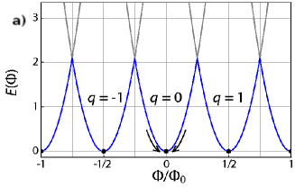
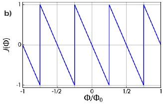
Figure 2: (a) Energy $E(\Phi)$ and (b) supercurrent $J(\Phi)$ as a function of flux $\Phi$ for a conventional superconducting loop at $T=0$. The minima in $E(\Phi)$ correspond to superconducting states with different pair momenta $q$. The screening currents in the superconductor drive the system to the closest minimum for each flux value (black points), if the walls of the loop are thicker than $\lambda$.

The two types of pairing states described above are qualitatively different. For the $\Phi_{0}/2$ periodicity, it is further required that the two types of states are degenerate. Byers and Yang as well as Brenig showed that this is indeed the case in the thermodynamic limit with a continuous density of states. The energy $E(\Phi)$ is then determined by a series of intersecting parabolae with minima at integer multiples of $\Phi_{0}$ (corresponding to even pair momenta $q$) and half integer multiples of $\Phi_{0}$ (corresponding to odd pair momenta $q$) [Fig. 2 (a)]. If the loop is thicker than $\lambda$, the system locks into the minimum closest to the value of the external flux. In finite systems however, the degeneracy of the even and odd $q$ minima is lifted, but their position is fixed by gauge invariance. The flux periodicity in thin loops is thus not necessarily $\Phi_{0}/2$, but the superconducting flux quantum remains $\Phi_{0}/2$. The circulating supercurrent $J(\Phi)$ is proportional to $\partial E(\Phi)/\partial\Phi$ and forms a $\Phi_{0}/2$ periodic saw-tooth pattern in the thermodynamic limit as shown in Fig. 2 (b).

II Flux periodicities in cylinders: An analytic approach

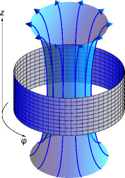
Figure 3: As a model system we use a thin-wall cylinder constructed from a two-dimensional discrete lattice. The interior of the cylinder is threaded by a magnetic flux $\Phi$; we assume that the flux does not penetrate into the cylinder wall. $\Phi$ can be chosen arbitrarily, since quantization applies to the fluxoid and not the flux itself.

For the discussion of the magnetic flux periodicity of $d$-wave superconductors we choose to bend a discrete two-dimensional $N\times M$ square lattice to a cylinder (Fig. 3) with circumference $Na$ and height $Ma$. For two reasons we expect nodal superconductors to support a $\Phi_{0}=hc/e$ rather than a $\Phi_{0}/2$ periodicity. The first arises from the discrete nature of the eigenenergies in a finite system. For the thin cylinder shown in Fig. 3 the mean level spacing in the vicinity of the Fermi energy $E_{\rm F}$ is $\delta_{F}\propto 1/(NM)$; in $s$-wave superconductors with an order parameter $\Delta\gg\delta_{F}$, $\delta_{F}$ matters little. For superconducting states with gap nodes, the situation is different. In $d$-wave superconductors with an order parameter $\Delta_{{\bf k}}\propto k_{\varphi}^{2}-k_{z}^{2}$, the nodal states closest to $E_{\rm F}$ have to fulfill the condition $k_{z}=k_{\varphi}$, thus there are fewer possible eigenstates and $\delta_{F}\propto 1/N$.

The second reason is that for gapless superconductors with a finite density of states close to $E_{\rm F}$, the occupation probabilities of these states change with flux. The flux dependence of the occupation enhances the difference of current matrix elements for integer and half-integer flux values loder:08 ; loder:08.2 ; juricic:07 ; barash:07 . This effect is best understood in terms of the spatial extent of a Cooper pair. In $s$-wave superconductors, the occupation probability remains constant for all $\Phi$, if the diameter of the cylinder is larger than the coherence length $\xi_{0}$. If this condition is fulfilled, the constituents of a Cooper pair cannot circulate separately, i.e. the pair does not feel the multiply connected geometry of the cylinder. But for nodal superconducting states, the lengthscale which characterizes their coherence, diverges in the nodal directions and there are always Cooper pairs which extend around the circumference of the cylinder. Therefore nodal superconductors have no characteristic length scale above which the superconducting state is unaffected by the geometry of the system. These two combined effects are investigated on the basis of an analytic model in Sec. II.2.

II.1 Superconductivity in a flux-threaded cylinder

The properties of a finite-size multiply connected superconductor depend sensitively on the discrete energy spectrum in the normal state. On the $N\times M$ square lattice, the flux values where levels cross have a high degeneracy for special ratios $N/M$; for $N=M$, the degree of degeneracy is $M$. For the latter case, the differences between the spectrum for integer and half-integer flux values are most pronounced. For $N=M\pm 1$, the spectrum is almost $\Phi_{0}/2$-periodic. Away from these special choices of $N$ and $M$, the degeneracies are lifted, indicated by the blue shaded patches in Fig. 4. The size of the normal persistent current circulating around the cylinder is controlled by the change of the density of states near $E_{\rm F}$ upon increasing $\phi=\Phi/\Phi_{0}$. Since normal persistent currents in clean metallic rings are typically $\Phi_{0}$ periodic AB ; washburn:92 , we will choose $N=M$ and a half-filled system with the chemical potential $\mu=0$ for our model study, where the $\Phi_{0}$ periodicity of the spectrum is most clearly established. Whenever an energy level crosses $E_{\rm F}$ with increasing flux, the current reverses its sign. The current is $\Phi_{0}$-periodic for even $N$ and either paramagnetic or diamagnetic in the vicinity of $\phi=0$. For odd $N$, the current is $\Phi_{0}/2$-periodic. This lattice-size dependence persists also in rings with electron-electron interactions fye ; Sharov:05 ; waintal or in mesoscopic superconducting islands mineev .

We choose in the following $N$ and $M$ even, which leads to a normal state spectrum of the type shown in Fig. 4. This is not an obvious choice, but we will see in chapter 3 that one obtains this type of spectrum also for a square loop to which we will compare the results obtained for the cylinder geometry.

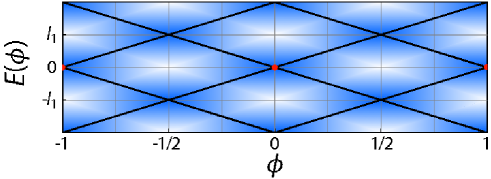
Figure 4: The energy spectrum of a cylinder in the normal state depends on the numbers $N$ and $M$, which parametrize the circumference and the height of the cylinder loder:09 . The black lines represent the energy levels for a one-dimensional ring with $M=1$ and $N$ an integer, where level crossings occur for integer values of $\phi=\Phi/\Phi_{0}$. $l_{1}$ is the maximum Doppler shift for $\phi=1/2$ (see Sec. II.2). For $M\gg 1$, the levels split and form a quasi continuous spectrum that depends on the ratio $N/M$ (blue patches).

The starting point for our analysiss is the BCS theory for a flux threaded cylinder with circumference $Na=2\pi Ra$ and height $Ma$, where $R$ is the dimensionless radius of the cylinder and $a$ the lattice constant. The pairing Hamiltonian is given by

$${\cal H}=\sum_{{\bf k},s}\epsilon_{\bf k}(\phi)c_{{\bf k}s}^{\dagger}c_{{\bf k}s}+\sum_{{\bf k}}\left[\Delta^{*}({\bf k},{\bf q})c_{{\bf k}\uparrow}c_{-{\bf k}+{\bf q}\downarrow}+\Delta({\bf k},{\bf q})c^{\dagger}_{-{\bf k}+{\bf q}\downarrow}c^{\dagger}_{{\bf k}\uparrow}\right],$$ (2)

where ${\bf k}=(k_{\varphi},k_{z})$ with $k_{\varphi}=n/R$ and $n\in\{-N/2+1,\dots,N/2\}$. The open boundary conditions in the $z$-direction along the axis of the cylinder allow for even-parity solutions with $k_{z}=(2m_{e}-1)\pi/M$ and odd-parity solutions with $k_{z}=2\pi m_{o}/M$, where $m_{e},m_{o}\in\{1,\dots,M/2\}$. The operators $c^{\dagger}_{{\bf k}s}$ and $c_{{\bf k}s}$ create and annihilate electrons with angular momentum $\hbar k_{\varphi}/a$ and momentum $\hbar k_{z}/a$ in $z$ direction. For convenience, we choose $k_{\varphi}$, $k_{z}\in[0,2\pi]$. The eigenenergies of free electrons moving on a discrete lattice on the surface of the flux threaded cylinder have the form

$$\epsilon_{\bf k}(\phi)=-2t\left[\cos\left(k_{\varphi}-\frac{\phi}{R}\right)+\cos k_{z}\right]-\mu.$$ (3)

For $R\gg 1$, $\epsilon_{\bf k}(\phi)$ is expanded to linear order in $\phi/R$;

$$\epsilon_{\bf k}(\phi)-\epsilon_{\bf k}(0)\approx-2t\frac{\phi}{R}\sin k_{\varphi}$$ (4)

is commonly called the Doppler shift.

The superconducting order parameter in the pairing Hamiltonian (2) is defined through

$$\Delta({\bf k},{\bf q})\equiv\Delta_{q}(\phi)g({\bf k}-{\bf q}/2)=\frac{1}{2}\sum_{{\bf k}^{\prime}}V({\bf k},{\bf k}^{\prime},{\bf q})\langle c_{-{\bf k}^{\prime}+{\bf q}\downarrow}c_{{\bf k}^{\prime}\uparrow}-c_{-{\bf k}^{\prime}+{\bf q}\uparrow}c_{{\bf k}^{\prime}\downarrow}\rangle,$$ (5)

where $V({\bf k},{\bf k}^{\prime},{\bf q})$ is the pairing interaction. Here we choose a $d$-wave interaction in separable form: $V({\bf k},{\bf k}^{\prime},{\bf q})=V_{1}g({\bf k}-{\bf q}/2)g({\bf k}^{\prime}-{\bf q}/2)$ with $g({\bf k})=\cos(k_{\varphi})-\cos(k_{z})$; $V_{1}$ is the pairing interaction strength Loder2010 . The order parameter $\Delta({\bf k},{\bf q})$ represents spin-singlet Cooper pairs with pair momentum $\hbar{\bf q}/a$. On the cylinder, the coherent motion of the Cooper pairs is possible only in the azimuthal direction, therefore ${\bf q}=(q/R,0)$ with $q\in\{-N/2+1,\dots,N/2\}$. The quantum number $q$ is obtained from minimizing the free energy. The $\phi$-dependence of $\Delta_{q}(\phi)$ enters through the self-consistency condition and has been discussed extensively in czajka:05 and loder:08.2 for $s$-wave pairing, where $g({\bf k})\equiv{\rm const}$. As verified numerically, $\Delta_{q}(\phi)$ varies only little with $\phi$, and we start our analytic calculation with a $\phi$ and $q$ independent order parameter $\Delta({\bf k},{\bf q})\equiv\Delta({\bf k})$ and $\Delta_{q}(\phi)\equiv\Delta$. As in our preceding work loder:08.2 , we take $q={\rm floor}(2\phi+1/2)$ in a first step. Since the Hamiltonian (2) is invariant under the simultaneous transformation $\phi\rightarrow\phi\pm 1$ and $q\rightarrow q\pm 2$, it is sufficient to consider $q=0$ or $1$ and the corresponding flux sectors $-1/4\leq\phi<1/4$ and $1/4\leq\phi<3/4$, respectively.

The diagonalization of the Hamiltonian (2) leads to the quasiparticle dispersion

$$E_{\pm}({\bf k},{\bf q},\phi)=\frac{\epsilon_{\bf k}(\phi)-\epsilon_{-{\bf k}+{\bf q}}(\phi)}{2}\pm\sqrt{\Delta^{2}({\bf k})+\epsilon^{2}({\bf k},{\bf q},\phi)},$$ (6)

with $\epsilon({\bf k},{\bf q},\phi)=[\epsilon_{\bf k}(\phi)+\epsilon_{-{\bf k}+{\bf q}}(\phi)]/2$. Expanding $E_{\pm}({\bf k},{\bf q},\phi)$ to linear order in both $\phi/R$ and $q/R$ gives

$$E_{\pm}({\bf k},{\bf q},\phi)\approx-e_{q}({\bf k})\pm\sqrt{\Delta^{2}({\bf k})+\left[\epsilon_{\bf k}(0)-l_{q}({\bf k})\right]^{2}},$$ (7)

where

$$e_{q}({\bf k})=\frac{\phi-q/2}{R}2t\sin k_{\varphi}\hskip 28.45274pt{\rm and}\hskip 28.45274ptl_{q}({\bf k})=\frac{tq}{R}\sin k_{\varphi}.$$ (8)

In the normal state $\Delta=0$, the additive combination of $e_{q}({\bf k})$ and $l_{q}({\bf k})$ leads to the ${\bf q}$-independent dispersion (3). For $\Delta>0$, the dispersion (7) differs for even and odd $q$, except for special ratios of $N$ and $M$, as discussed above. This difference is crucial for nodal superconductors: The condition $k_{\varphi}\approx k_{z}$ for levels close to $E_{\rm F}$ causes a level spacing $\delta_{F}\approx 2l_{1}({\bf k}_{F})$ for small $\Delta$, where ${\bf k}_{F}$ is the Fermi momentum. For $N$ and $M$ even and $q=0$, the degenerate energy level at $E=E_{\rm F}=0$ splits into $M$ levels for increasing $\Delta$, which spread between $-\Delta$ and $\Delta$. For $q=1$, the degenerate levels closest to $E_{\rm F}$ are located at $E=\pm|l_{1}({\bf k}_{F})|$, thus a gap of $2l_{1}({\bf k}_{F})$ remains in the superconducting spectrum. If $N$ and $M$ are odd, the spectra for even and odd $q$ are interchanged, and if either $N$ or $M$ is odd, the spectrum is a superposition.

The gauge invariant circulating supercurrent is given by

$$J(\phi)=\frac{e}{h}\sum_{{\bf k},s}v_{\bf k}n_{s}({\bf k}),$$ (9)

where $v_{\bf k}={\partial\epsilon_{\bf k}(\phi)}/{\partial(Rk_{\varphi})}$ is the group velocity of the single-particle state with eigenenergy $\epsilon_{\bf k}(\phi)$. The spin independent occupation probability of this state is

$$n_{s}({\bf k})=\langle c_{{\bf k}s}^{\dagger}c_{{\bf k}s}\rangle=u^{2}({\bf k},{\bf q},\phi)f(E_{+}({\bf k},{\bf q},\phi))+v^{2}({\bf k},{\bf q},\phi)f(E_{-}({\bf k},{\bf q},\phi))$$ (10)

with the Fermi function $f(E)$ and the Bogoliubov amplitudes

$$u^{2}({\bf k},{\bf q},\phi)=\frac{1}{2}\left[\frac{\epsilon({\bf k},{\bf q},\phi)}{E({\bf k},{\bf q},\phi)}+1\right]\hskip 28.45274pt{\rm and}\hskip 28.45274ptv^{2}({\bf k},{\bf q},\phi)=\frac{1}{2}\left[\frac{\epsilon({\bf k},{\bf q},\phi)}{E({\bf k},{\bf q},\phi)}-1\right].$$ (11)

From Eqs. (9) and (10), the supercurrent in the cylinder is obtained by evaluating the sum either numerically or from the approximative analytic solution in Sec. II.2, which allows insight into the origin of the $\Phi_{0}$-periodicity in nodal superconductors. First, the analytic solution, which was introduced in Ref. loder:09 , is reviewed.

II.2 Analytic solution and qualitative discussion

An analytic evaluation of the supercurrent is possible in the thermodynamic limit where the sum over discrete eigenstates is replaced by an integral. For a multiply connected geometry, this limit is not properly defined because the supercurrent or the Doppler shift vanish in the limit $R\rightarrow\infty$. Care is needed to modify the limiting procedure in a suitable way to access the limit of a large but non-infinite radius of the cylinder loder:09 . In this limit it is mandatory to consider the supercurrent density $j(\phi)=J(\phi)/M$ rather than the supercurrent $J(\phi)$. In this scheme, we treat the density of states as a continuous function in any energy range where the level spacing is $\propto 1/NM$, but we keep the finite energy gap of width $2l_{q}({\bf k}_{F})\propto 1/R\propto 1/N$ around $E_{\rm F}$ in the odd-$q$ sectors. For the tight-binding dispersion in Eq. (3), the density of states is a complete elliptic integral of the first kind. For the purpose of an analytic calculation, a quadratic dispersion with a constant density of states is therefore a more suitable starting point. We use the expanded form of Eq. (3):

$$\epsilon_{\bf k}(\phi)=t\left[\left(k_{\varphi}-\frac{\phi}{R}\right)^{2}+k_{z}^{2}\right]-\mu^{\prime},$$ (12)

where $\mu^{\prime}=\mu+4t$.

Some algebraic steps are needed to rearrange the sum in Eq. (9) suitably to convert it into an integral. For finite $\phi$, $\epsilon_{\bf k}(\phi)\neq\epsilon_{-{\bf k}}(\phi)$, and consequently the sum has to be decomposed into contributions with $k_{\varphi}\geq 0$ and $k_{\varphi}<0$. We therefore take $k_{\varphi}\geq 0$ and decompose $v_{\bf k}$ as

$$v_{\pm{\bf k}}=\frac{2t}{R}\left(\pm k_{\varphi}-\frac{\phi}{R}\right)=v_{d}({\bf k})\pm v_{p}({\bf k}),$$ (13)

into a diamagnetic contribution $v_{d}({\bf k})=-2t\phi/R^{2}$ and a paramagnetic contribution $v_{p}({\bf k})=2tk_{\varphi}/R$ scalapino:93 .

In a continuous energy integration, the Doppler shift is noticeable only in the vicinity of $E_{\rm F}$. On the Fermi surface $k_{\varphi}$ and $k_{z}$ are related by

$$k_{\varphi,F}(k_{z})=\sqrt{\frac{\mu^{\prime}}{t}-k_{z}^{2}}.$$ (14)

We therefore approximate $e_{q}({\bf k})$ and $l_{q}({\bf k})$ by $e_{q}(k_{z})\approx 2t(\phi-q/2)k_{\varphi,F}(k_{z})/R$ and $l_{q}(k_{z})\approx tqk_{\varphi,F}(k_{z})/R$, respectively. The eigenenergies (7) near $E_{\rm F}$ are thereby rewritten as

$$E_{+}(\pm k_{\varphi},k_{z},{\bf q},\phi)=\mp e_{q}(k_{z})+\sqrt{\Delta_{\bf k}^{2}+\left(\epsilon_{\bf k}(0)\mp l_{q}(k_{z})\right)^{2}}$$

$$E_{-}(\pm k_{\varphi},k_{z},{\bf q},\phi)=\mp e_{q}(k_{z})-\sqrt{\Delta_{\bf k}^{2}+\left(\epsilon_{\bf k}(0)\mp l_{q}(k_{z})\right)^{2}}$$ (15)

The supercurrent $J(\phi)$ in Eq. (9) is now evaluated by an integral over $k_{\varphi}$ and $k_{z}$, which is decomposed into an integral over the normal state energy $\epsilon$ and an angular variable $\theta$. Within this scheme the density of states becomes gapless in the limit $M\rightarrow\infty$ for $q=0$, although $N$ is kept finite. For $q=1$ instead, a $k_{z}$-dependent gap $2|l_{1}(k_{z})|$ remains. Thus we replace $\epsilon_{\bf k}(0)\mp|l_{q}(k_{z})|$ by the continuous quantity $\epsilon\pm|l_{q}(E_{\rm F},\theta)|$ where we use the parametrization

$$\left(\begin{array}[]{l}k_{\varphi}\\ k_{z}\end{array}\right)=\left(\begin{array}[]{l}k\cos\theta\\ k\sin\theta\end{array}\right)=\sqrt{\frac{\epsilon+\mu^{\prime}}{t}}\left(\begin{array}[]{l}\cos\theta\\ \sin\theta\end{array}\right),$$ (16)

with $\epsilon=tk^{2}-\mu^{\prime}$. The energy integral extends over the whole tight-binding band width with $E_{\rm F}=0$ in the center of the band. Correspondingly, we integrate from $-\mu^{\prime}$ to $\mu^{\prime}$. Furthermore, the Doppler shift is parametrized for $\epsilon\approx E_{\rm F}$ as

$$e_{q}(\theta)=\frac{\phi-q/2}{R}2t\sqrt{\mu^{\prime}/t}\cos\theta\hskip 42.67912pt{\rm and}\hskip 42.67912ptl_{q}(\theta)=\frac{tq}{R}\sqrt{\mu^{\prime}/t}\cos\theta,$$ (17)

where the function $l_{q}(\theta)$ is positive for $|\theta|\leq\pi/2$. The supercurrent thus becomes

$$j(\phi) =\frac{1}{M}\frac{e}{h}\left[\sum_{k_{\varphi}>0,k_{z},s}v_{\bf k}n_{{\bf k}s}({\bf q})+\sum_{k_{\varphi}<0,k_{z},s}v_{\bf k}n_{{\bf k}s}({\bf q})\right]$$ (18)

$$\approx 2{\cal N}\frac{e}{h}\!\int_{-\pi/2}^{\pi/2}\!\!{\rm d}\theta\int_{-\mu^{\prime}}^{\mu^{\prime}}\!{\rm d}\epsilon[n_{q+}(\epsilon,\theta)v_{+}(\epsilon,\theta)+n_{q-}(\epsilon,\theta)v_{-}(\epsilon,\theta)],$$

where $n_{q\pm}(\epsilon,\theta)=n_{\pm{\bf k}(\epsilon,\theta)}({\bf q})$ and $v_{\pm}(\epsilon,\theta)=v_{\pm{\bf k}(\epsilon,\theta)}$. The constant density of states in the normal state is ${\cal N}=R/4\pi t$. We collect the terms proportional to $v_{d}(\epsilon,\theta)=-2t\phi/R^{2}$ into a diamagnetic current contribution $j_{\rm d}$ and those proportional to $v_{p}(\epsilon,\theta)=2tk_{\varphi,F}(\epsilon,\theta)/R$ into a paramagnetic contribution $j_{\rm p}$. Using $f(-E)=1-f(E)$, $j_{\rm d}$ and $j_{\rm p}$ become

$$j_{\rm d}(q,\phi) =4{\cal N}\frac{e}{h}\!\int_{-\pi/2}^{\pi/2}{\rm d}\theta\int_{l_{q}(\theta)}^{\mu^{\prime}}{\rm d}\epsilon\,v_{d}\left(\epsilon,\theta\right)\frac{\epsilon}{\sqrt{\Delta^{2}+\epsilon^{2}}}\left[f(E+e_{q}(\theta))-f(-E+e_{q}(\theta))\right],$$ (19)

$$j_{\rm p}(q,\phi) =4{\cal N}\frac{e}{h}\!\int_{-\pi/2}^{\pi/2}{\rm d}\theta\int_{l_{q}(\theta)}^{\mu^{\prime}}{\rm d}\epsilon\,v_{p}\left(\epsilon,\theta\right)\left[f(-E-e_{q}(\theta))-f(-E+e_{q}(\theta))\right],$$ (20)

Here, the integration is over positive $\epsilon$ only, and the lower boundary of the energy integration is controlled by $l_{q}(\theta)$. In Eq. (19) we used the abbreviations $\Delta=\Delta(\theta)$ and $E=E(\epsilon,\theta)=\sqrt{\Delta^{2}(\theta)+\epsilon^{2}}$. The current $j_{\rm d}$ is diamagnetic in the even-$q$ flux sectors and paramagnetic in the odd-$q$ sectors. For even $q$, it is equivalent to the diamagnetic current obtained from the London equations pethick:79 ; tinkham . The current $j_{\rm p}$ has always the reverse sign of $j_{\rm d}$ and is related to the quasiparticle current as shown below. To analyze the flux dependent properties of the spectra and the current in the even-$q$ and odd-$q$ sectors, we explicitly distinguish $s$-wave pairing and $d$-wave pairing with nodes in the gap function.

II.2.1 $s$-wave pairing symmetry

For $s$-wave pairing, $\Delta(\epsilon,\theta)\equiv\Delta$ is constant. Therefore, if we assume that $\Delta\geq e_{q}(\theta)$ for all $\theta$, the lower energy integration boundary in Eqs. (19) and (20) is $\Delta$. Thus $j(\phi)=j_{\rm d}+j_{\rm p}$ is equal in both the even-$q$ and the odd-$q$ flux sectors and the flux periodicity is $\Phi_{0}/2$. However, if $\Delta<\max_{\theta}e_{q}(\theta)$, different calculational steps have to be followed in the evaluation of Eq. (9), the results of which have been presented in loder:08.2 .

With $\epsilon=\sqrt{E^{2}-\Delta^{2}}$, Eqs. (19) and (20) transform into integrals over $E$ with ${\rm d}\epsilon=D_{s}(E)\,{\rm d}E$, where

$$D_{s}(E)=\frac{\partial\epsilon}{\partial E}=\left\{\begin{array}[]{lll}E\,(E^{2}-\Delta^{2})^{-1/2}\hskip 14.22636pt{\rm for}\hskip 14.22636ptE\geq\Delta\\ 0\hskip 82.51282pt{\rm for}\hskip 14.22636ptE<\Delta\end{array}\right.$$ (21)

is the density of states for $s$-wave pairing. This leads to

$$j_{\rm d} = 4{\cal N}\frac{e}{h}\!\int_{-\pi/2}^{\pi/2}{\rm d}\theta\int_{\Delta}^{\mu^{\prime}}{\rm d}Ev_{d}\left(\sqrt{E^{2}-\Delta^{2}},\theta\right)\left[f(E+e_{q}(\theta))-f(-E+e_{q}(\theta))\right],$$ (22)

$$j_{\rm p} = 4{\cal N}\frac{e}{h}\!\int_{-\pi/2}^{\pi/2}{\rm d}\theta\int_{\Delta}^{\mu^{\prime}}{\rm d}ED_{s}(E)v_{p}\left(\sqrt{E^{2}-\Delta^{2}},\theta\right)\left[f(-E-e_{q}(\theta))\!-\!f(-E+e_{q}(\theta))\right].$$ (23)

At $T=0$, we obtain

$$j_{\rm d} = -4{\cal N}\frac{e}{h}\!\int_{-\pi/2}^{\pi/2}{\rm d}\theta\int_{\Delta}^{\mu^{\prime}}{\rm d}E\,2t\frac{\phi-q/2}{R^{2}}=-2(\mu^{\prime}-\Delta)\frac{e}{h}\frac{\phi-q/2}{R},$$ (24)

$$j_{\rm p} = 4{\cal N}\frac{e}{h}\!\int_{-\pi/2}^{\pi/2}{\rm d}\theta\int_{\Delta}^{e_{q}(\theta)}{\rm d}ED_{s}(E)\frac{2t}{R}\sqrt{\frac{\epsilon+\mu^{\prime}}{t}}\cos\theta$$ (25)

$$= \frac{8t{\cal N}}{R}\frac{e}{h}\sqrt{\frac{\mu^{\prime}}{t}}\int_{-\pi/2}^{\pi/2}{\rm d}\theta\cos\theta\int_{\Delta}^{e_{q}(\theta)}{\rm d}ED_{s}(E)+{\cal O}\left(\frac{\epsilon}{t}\right)^{2}.$$

The current $j_{\rm d}$ becomes independent of the superconducting density of states. Its size is proportional to $E_{\rm F}$, as long as $\mu^{\prime}\gg\Delta$ holds.

If $\Delta>e_{q}(\theta)$ for all values of $\theta$, then $j_{\rm p}=0$ and the supercurrent $j(\phi)=j_{\rm d}$ is diamagnetic. For $T>0$, $j_{\rm d}$ decreases slightly. The current $j_{\rm p}$ increases with increasing $T$ and reaches its maximum value at $T_{\rm c}$. For finite temperatures $j_{\rm p}$ is referred to as the quasiparticle current. The supercurrent is always the sum of the diamagnetic current $j_{\rm d}$ and the quasiparticle current $j_{\rm p}$, and therefore decreases with increasing temperature and vanishes at $T_{\rm c}$ vonoppen:92 . The quasiparticle current has the same flux periodicity as the supercurrent, even though it is carried by quasiparticle excitations. In the normal state ($\Delta=0$),

$$j_{\rm p}=\frac{8t{\cal N}}{R}\frac{e}{h}\sqrt{\frac{\mu^{\prime}}{t}}\int_{-\pi/2}^{\pi/2}{\rm d}\theta\cos\theta\int_{0}^{e_{q}(\theta)}{\rm d}E=4\mu^{\prime}\frac{e}{h}\frac{\phi-q/2}{R\pi}\int_{-\pi/2}^{\pi/2}{\rm d}\theta\cos^{2}\theta=2\mu^{\prime}\frac{e}{h}\frac{\phi-q/2}{R}$$ (26)

which cancels $j_{\rm d}$ exactly in the limit $M\rightarrow\infty$.

II.2.2 Unconventional pairing with gap nodes

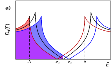
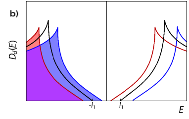
Figure 5: Scheme for the density of states of a $d$-wave superconductor for $\phi=1/4$, where $e_{q}=l_{1}/2$ loder:09 . The center-of-mass angular momentum $\hbar q/aR$ of the Cooper pairs is (a) $q=0$ and (b) $q=1$. The energies are Doppler shifted to higher (red) or lower energies (blue). This results in a double-peak structure; for $q=0$ the upper and lower band overlap in the region $-e_{0}<E<e_{0}$ khavkine:04 and states in the upper band become partially occupied. For $q=1$ there is a gap $l_{1}$ of the size of the maximum Doppler shift at $\phi=1/4$. The black line represents the density of states (a) for $\phi=0$ and (b) for $\phi=1/2$.

Equation (24) for $j_{\rm d}$ is valid also for unconventional order parameter symmetries. Physically, $j_{\rm d}$ reflects the difference in the density of states of quasiparticle states with orbital magnetic moments parallel and anti-parallel to the external magnetic field. The former states are Doppler shifted to lower energies, whereas the latter are Doppler shifted to higher energies. This is schematically shown in Fig. 5 for $d$-wave pairing (c.f. khavkine:04 ). In this picture, $j_{\rm d}$ is proportional to the difference between the area beneath the red and and blue curves representing the density of states arising from $E_{-}(\pm|{\bf k}|,{\bf q},\phi)<0$. Therefore we approximate $j_{\rm d}$ for $\Delta(\theta)\ll\mu^{\prime}=E_{\rm F}+4t$ by

$$j_{\rm d}=-2\mu^{\prime}\frac{e}{h}\frac{\phi-q/2}{R},$$ (27)

as given in equation (24) with $\Delta=0$. On the other hand, $j_{\rm p}$ is represented by the occupied quasiparticle states in the overlap region of $E_{+}({\bf k},{\bf q},\phi)$ and $E_{-}({\bf k},{\bf q},\phi)$ with width $2e_{q}({\bf k}_{F})$. It therefore strongly depends on the density of states in the vicinity of $E_{\rm F}$. In Fig. 5 (a), which refers to even $q$, the current $j_{\rm p}$ is determined by the small triangular patch where the upper and lower bands overlap. For odd $q$, the two bands do not overlap, therefore $j_{\rm p}=0$.

We will now analyze such a scenario for $d$-wave pairing with an order parameter $\Delta_{\bf k}=\Delta(k_{\varphi}^{2}-k_{z}^{2})\approx\Delta\cos 2\theta$. Again, we assume $\Delta>e_{q}(\theta)$ for all $\theta$; then the integral in Eq. (20) contains only the nodal states closest to $E_{\rm F}$, for which the $d$-wave symmetry demands $k_{\varphi}\approx k_{z}$. Jointly with Eq. (14) this condition fixes the Doppler shift at $E_{\rm F}$ to the ${\bf k}$-independent value $e_{q}=(\phi-q/2)\sqrt{2t\mu^{\prime}}/R$ and $l_{q}=(q/R)\sqrt{t\mu^{\prime}/2}$. With the density of states

$$D_{d}(E)=\frac{1}{\sqrt{E^{2}-\Delta^{2}\cos^{2}2\theta}},$$ (28)

Eq. (20) for the paramagnetic current $j_{\rm p}$ at $T=0$ takes the form

$$j_{\rm p}=4{\cal N}\frac{e}{h}\!\int_{l_{q}}^{e_{q}}{\rm d}E\int_{-\pi/2}^{\pi/2}{\rm d}\theta D_{d}(E)\frac{2t}{R}\sqrt{\frac{\epsilon+\mu^{\prime}}{t}}\sin\theta.$$ (29)

In the odd-$q$ flux sectors, $l_{q}\geq e_{q}$ for all values of $\phi$, therefore $j_{\rm p}=0$. In the $q=0$ sector, $l_{q}=0$ and

$$j_{\rm p}\approx\frac{2e}{h\pi}\sqrt{\frac{\mu^{\prime}}{t}}\int_{0}^{e_{q}}{\rm d}E\int_{-\pi/2}^{\pi/2}{\rm d}\theta\sin\theta\frac{1}{\sqrt{E^{2}-\Delta^{2}\cos^{2}2\theta}}\approx\frac{2e}{\pi h}\sqrt{\frac{\mu^{\prime}}{t}}\int_{0}^{e_{q}}{\rm d}E\frac{E}{\Delta}$$

$$=\frac{e}{\pi h\Delta}\sqrt{\frac{\mu^{\prime}}{t}}e_{q}^{2}=\frac{2}{\pi\Delta}\sqrt{t\mu^{\prime 3}}\frac{e}{h}\left(\frac{\phi-q/2}{R}\right)^{2},$$ (30)

where the same approximations as in the $s$-wave case are applied. The dominant contribution to the integral over $\theta$ originates from the nodal parts (see e.g. mineev ).

In the even-$q$ sectors, the total current $j(\phi)=j_{\rm d}+j_{\rm p}$ becomes

$$j(\phi)=-2\mu^{\prime}\frac{e}{h}\frac{\phi}{R}\left[1-\frac{\sqrt{t\mu^{\prime}}}{\pi\Delta}\frac{\phi}{R}\right],$$ (31)

which results in the ratio of the two current components

$$\frac{j_{\rm p}}{j_{\rm d}}=\frac{\sqrt{t\mu^{\prime}}}{\pi\Delta}\frac{\phi}{R}\equiv b\phi.$$ (32)

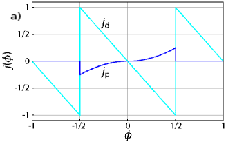
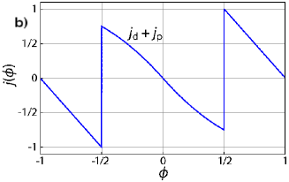
Figure 6: The supercurrent density $j(\phi)=j_{\rm d}+j_{\rm p}$ in a thin $d$-wave cylinder as a function of flux $\phi$ (arbitrary units) loder:09 . Shown is the result of the analytic model calculation [Eq. (33)] for the characteristic value $b=0.4$. For $-1/4<\phi<1/4$, where $q=0$, the current is reduced by a contribution proportional to $\phi^{2}$, whereas it is linear in $\phi$ otherwise. This leads to an overall flux periodicity of $\Phi_{0}$.

In the odd-$q$ flux sectors $j_{\rm p}=0$ and the supercurrent is $j(\phi)=j_{\rm d}$. $j(\phi)$ is consequently $\Phi_{0}$ periodic; within one flux period from $-1/2$ to $1/2$ we represent it as

$$j(\phi)=-2\frac{\mu^{\prime}}{R}\frac{e}{h}\left\{\begin{array}[]{llrl}\phi+1/2&{\rm for}&-1/2\leq&\phi<-1/4,\\ \phi(1-b\phi)&{\rm for}&-1/4\leq&\phi<1/4,\\ \phi-1/2&{\rm for}&1/4\leq&\phi<1/2,\end{array}\right.$$ (33)

(c.f. Fig. 6). The difference of the supercurrent in the even-$q$ and odd-$q$ flux sectors is represented best by the Fourier components $j_{n}=\int_{-1/2}^{1/2}{\rm d}\phi\;j(\phi)e^{2\pi in\phi}$. For the first ($j_{1}$) and the second Fourier component ($j_{2}$) we obtain

$$j_{1}=-2\frac{\mu^{\prime}}{R}\frac{e}{h}b\frac{8-\pi^{2}}{16\pi^{3}}\hskip 28.45274pt{\rm and}\hskip 28.45274ptj_{2}=-2\frac{\mu^{\prime}}{R}\frac{e}{h}\frac{4\pi i-b}{16\pi^{2}}.$$ (34)

To leading order in $1/R$, the ratio of the $\Phi_{0}$ and the $\Phi_{0}/2$ Fourier component is therefore

$$\left|\frac{j_{1}}{j_{2}}\right|=\frac{\pi^{2}-8}{4\pi^{2}}\frac{\sqrt{2t\mu^{\prime}}}{\Delta R},\hskip 42.67912pt\lim_{\mu\rightarrow 0}\left|\frac{j_{1}}{j_{2}}\right|\approx 0.07\frac{2t}{\Delta R},$$ (35)

and scales with the inverse ring diameter. This $1/R$-law is the direct consequence of the $d$-wave density of states $D_{d}(E)\propto E$. Using Eq. (35) to estimate this ratio for a mesoscopic cylinder with a circumference $Ra=2600a\approx 1\,\mu$m and a ratio $\Delta/t=0.01$, we obtain $j_{1}/j_{2}\approx 0.03$.

II.3 Further aspects

We have shown that in rings of unconventional superconductors with gap nodes, there is a paramagnetic, quasiparticle-like contribution $j_{\rm p}>0$ to the supercurrent at $T=0$. This current is generated by the flux-induced reoccupation of nodal quasiparticle states slightly below and above $E_{\rm F}$. Formally a coherence length $\hbar v_{F}/\Delta({\bf k},{\bf q})>2R$ can be ascribed to these reoccupied states, which are therefore affected by the symmetry of the system. If the normal state energy spectrum has a flux periodicity of $\Phi_{0}$, than the superconducting spectrum is $\Phi_{0}$ periodic, too. The normal state spectrum of a cylinder with a discrete lattice strongly depends on the number of lattice sites. This problem is characteristic for rotationally symmetric systems and is much less pronounced in geometries with lower symmetry, such as the square frame discussed in Sec. 3. In the latter system impurities do not change the spectrum qualitatively. For modelling an experimental arrangement a square loop geometry is therefore preferable.

The $\Phi_{0}$ periodicity is best visible in the current component $j_{\rm p}$ at $T=0$. For $d$-wave-pairing $j_{\rm p}\propto 1/R^{2}$, and the $\Phi_{0}$ periodic Fourier component decays like the inverse radius of the cylinder, relative to the $\Phi_{0}/2$ periodic Fourier component. The lack of a characteristic length scale in nodal superconductors, such as the coherence length for $s$-wave pairing, generates this algebraic decay. Although $j_{\rm p}$ is larger for small $\Delta$, it almost vanishes close to $T_{\rm c}$, if $\Delta\gg\delta_{F}$, and variations of $T_{\rm c}$ with flux, as in the Little-Parks experiment Little ; Parks , do not differ for $s$- and $d$-wave superconductors.

III Flux periodicity in square frames: Bogoliubov – de Gennes approach

So far we have presented the principles of the crossover from $\Phi_{0}$ to $\Phi_{0}/2$ flux periodicity in conventional and unconventional superconductors and the mechanisms that leads to the persistence of $\Phi_{0}$ periodicity in large loops of nodal superconductors. Now we present an alternative approach in real space via the Bogoliubov – de Gennes equations, which we introduce in Sec. III.1. The information we obtain from this technique is complementary to Sec. II where we followed the momentum-space formulation. The latter proved useful to understand the physical concepts and to describe large systems. The price paid was the restriction to highly symmetric systems with intriguing energy spectra in the normal state. This raises the question whether the $\Phi_{0}$ periodicity is detectable in realistic setups, or whether it is rather an artifact of the high degeneracy of energy levels in clean and highly symmetric systems? On the other hand, the Bogoliubov – de Gennes equations in real space allow to determine the spectrum of “natural” system geometries with reduced symmetry or systems containing lattice defects, impurities, magnetic fields or correlations in real space. Limitations of computational power, however, restrict the system size, and therefore the particular effects introduced by discreteness are unavoidably present.

The combination of momentum- and real-space methods can provide answers to the questions above. In the following, we first discuss the multi-channel loop for a square lattice: a square frame, as shown in Fig. 7, with a square hole at the center, threaded by a magnetic flux $\Phi$. We use this system in Sec. III.2 to study the flux periodicity in clean symmetric square frames; a part of this section is contained in loder:08 . In Sec. IV, we investigate different Josephson junction devices that respond periodically to magnetic fields. Junctions are modeled in real space by inserting potential barriers. In this context, we investigate also the effect of impurities and lattice defects on the energy spectrum of the square frame.

III.1 The Bogoliubov – de Gennes equations

The Hamiltonian which we use in the following section has the form

$${\cal H}=\!\sum_{\langle ij\rangle,s}t_{ij}c^{\dagger}_{is}c_{js}+\!\sum_{i}\left[\Delta^{\!*}_{i}c_{i\downarrow}c_{i\uparrow}+\Delta_{i}c^{\dagger}_{i\uparrow}c^{\dagger}_{i\downarrow}\right]+\!\sum_{\langle ij\rangle}\left[\Delta^{\!*}_{ji}c_{j\downarrow}c_{i\uparrow}+\Delta_{ij}c^{\dagger}_{i\uparrow}c^{\dagger}_{j\downarrow}\right]+\!\sum_{i,s}(U_{i}-\mu)c^{\dagger}_{is}c_{is},$$ (36)

where $c^{\dagger}_{is}$, $c_{is}$ are creation and annihilation operators for an electron on lattice site $i$ with spin $s$, and $\mu$ is the chemical potential. The sum $\sum_{i}$ runs over all lattice sites and the sum $\sum_{\langle ij\rangle}$ is restricted to nearest-neighbor sites $i$ and $j$ only, and $t_{ij}=te^{\varphi_{ij}}$ with the hopping amplitude $t$ and the Peierls phase factor

$$\varphi_{ij}=\frac{e}{\hbar c}\int_{i}^{j}{\rm d}{\bf r}\cdot{\bf A}({\bf r}).$$ (37)

Additionally, we include an impurity term consisting of potential scatterers with repulsive potentials $U_{i}>0$, which we align to model tunnel junctions. A Hamiltonian of the form (36) has often been used before for the numeric investigation of vortices in $d$-wave superconductors and the technique is described in detail in a number of articles soininen:94 ; wang:95 ; zhu:00 ; Zhu:01 ; ghosal:02 ; chen:03 .

In the Hamiltonian Eq. (36) two types of spin-singlet pairing are included. The on-site order parameter $\Delta_{i}$ represents conventional $s$-wave pairing originating from an on-site interaction. The order parameter $\Delta_{ij}$ originates from a nearest-neighbor interaction between the sites $i$ and $j$. They are defined through

$$\Delta_{i}=V_{0}\langle c_{i\downarrow}c_{i\uparrow}\rangle\quad{\rm and}\quad\Delta_{ij}=\frac{V_{1}}{2}\left[\langle c_{j\downarrow}c_{i\uparrow}\rangle-\langle c_{i\downarrow}c_{j\uparrow}\rangle\right].$$ (38)

with the interaction strengths $V_{0}$ and $V_{1}$. To diagonalize the Hamiltonian (36) we use the Bogoliubov transformation

$$c_{i\uparrow}=\sum_{n}\left[u_{n_{i}}a_{n\uparrow}-v^{*}_{n_{i}}a^{\dagger}_{n\downarrow}\right],\hskip 42.67912ptc_{i\downarrow}=\sum_{n}\left[u_{n_{i}}a_{n\downarrow}+v^{*}_{n_{i}}a^{\dagger}_{n\uparrow}\right],$$ (39)

where the coefficients $u_{n_{i}}$ and $v_{n_{i}}$ are obtained from the eigenvalue equation

$$\left(\begin{array}[]{c@{\quad}c}{\hat{t}}&{\hat{\Delta}}\\ {\hat{\Delta}^{\!*}}&-\hat{t}^{*}\end{array}\right){{\bf u}_{n}\choose{\bf v}_{n}}=E_{n}{{\bf u}_{n}\choose{\bf v}_{n}}.$$ (40)

The operators $\hat{t}$ and $\hat{\Delta}$ act on the vectors ${\bf u}_{n}$ and ${\bf v}_{n}$ as

$$\hat{t}u_{n_{i}}=\sum_{j}t_{ij}u_{nj}+(U_{i}-\mu)u_{n_{i}}\quad{\rm and}\quad\hat{\Delta}v_{n_{i}}=\Delta_{i}v_{n_{i}}+\sum_{j}\Delta_{ij}v_{nj},$$ (41)

where $j$ labels the nearest-neighbor sites of site $i$. Inserting the transformation (39) into Eq. (38) leads to the self-consistency conditions

$$\Delta_{i}=V_{0}\sum_{n}u_{n_{i}}v^{*}_{n_{i}}\tanh\left(\frac{E_{n}}{2T}\right)\;,\qquad\Delta_{ij}=\frac{V_{1}}{2}\sum_{n}\left[u_{n_{i}}v^{*}_{nj}+u_{nj}v^{*}_{n_{i}}\right]\tanh\left(\frac{E_{n}}{2T}\right).$$ (42)

Equations (42) together with Eq. (40) represent the Bogoliubov – de Gennes equations.

The bond order parameters $\Delta_{ij}$ can be projected onto a $d$-wave component and an extended $s$-wave component defined as

$$\Delta^{s}_{i}=\frac{1}{4}\left[\Delta_{i,i+\hat{x}}e^{i\varphi_{i,i+\hat{x}}}+\Delta_{i,i-\hat{x}}e^{i\varphi_{i,i-\hat{x}}}+\Delta_{i,i+\hat{y}}e^{i\varphi_{i,i+\hat{y}}}+\Delta_{i,i-\hat{y}}e^{i\varphi_{i,i-\hat{y}}}\right],$$ (43)

$$\Delta^{d}_{i}=\frac{1}{4}\left[\Delta_{i,i+\hat{x}}e^{i\varphi_{i,i+\hat{x}}}+\Delta_{i,i-\hat{x}}e^{i\varphi_{i,i-\hat{x}}}-\Delta_{i,i+\hat{y}}e^{i\varphi_{i,i+\hat{y}}}-\Delta_{i,i-\hat{y}}e^{i\varphi_{i,i-\hat{y}}}\right].$$ (44)

In a uniform system with nearest-neighbor pairing interaction only, the self-consistency Eq. (42) selects a pure $d$-wave superconducting state, i.e. $\Delta^{s}_{i}=0$. Impurities, potentials or boundaries generate an extended $s$-wave contribution $\Delta^{s}_{i}>0$ franz:96 . The expectation value of the current $J_{ij}$ (cf. bagwell:94 ) from site $i$ to $j$ is given by

$$J_{ij}=-8t\,\Phi_{0}\sum_{n}\mbox{Im}\left(u_{nj}u_{in}^{*}e^{-i\varphi_{ij}}\right)f(E_{n}).$$ (45)

III.2 Flux periodicity in square frames

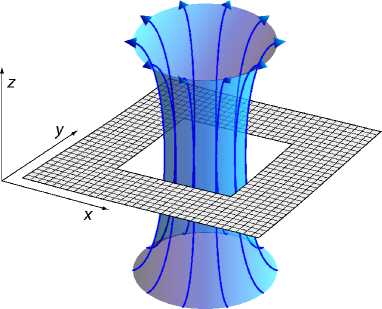
Figure 7: Illustration of a square loop threaded by a magnetic flux. For the investigation of the flux periodicity of $d$-wave superconductors using the Bogoliubov – de Gennes equations in real space, we use a discrete square lattice with open boundary conditions and a square hole in the center the frame, which is pierced by the magnetic flux $\Phi$.

The Bogoliubov – de Gennes equations introduced above are now applied to the square frame geometry shown in Fig. 7, consisting of a discrete $N\times N$ lattice with a centered $L\times L$ square hole threaded by a magnetic flux $\phi$, where $\phi=\Phi/\Phi_{0}$. The external magnetic field ${\bf B}$ threading the hole is supposed not to penetrate into the frame, and we restrict it to the center of the hole. ${\bf B}$ is generated by a vector potential of the form ${\bf A}({\bf r})=2\pi\phi/|{\bf r}|^{2}(y,-x,0)$.

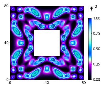
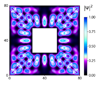
Figure 8: Real-space representations of a square loop with a typical electronic probability density $|\Psi|^{2}$. We show two eigenstates of the $d$-wave pairing Hamiltonian with slightly different energies in the gap region, calculated for a square-loop with 80$\times$80 lattice sites and a pairing interaction $V_{1}=0.3t$. The hole in the center has a size of 28$\times$28 unit cells. To enhance the contrast of the complicated pattern, the special color code shown on the right is used and the discrete lattice points are smoothly interpolated.

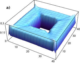
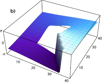
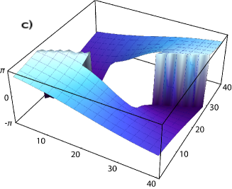
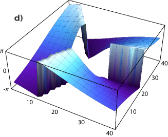
Figure 9: (a) Absolute value of the $d$-wave order parameter $\Delta^{d}_{i}$ (in units of $t$) in a $40\times 40$ square frame with a $14\times 14$ hole at the center for $q=0$, $\phi=0$, and $V_{1}=0.3t$. For this interaction strength, the suppression of $\Delta^{d}_{i}$ for $\phi\neq 0$ is small and not visible in this plot. The phase of $\Delta^{d}_{i}$ is shown for winding numbers $q=1,2,3$ in (b), (c) and (d), respectively.

In the normal state the Bogoliubov – de Gennes equations reduce to the discrete Laplace equation. While the low-energy states do not differ much from free plane waves, the higher-energy states near $E_{F}$ on the square frame develop some peculiar, frame-specific features. The wavelength of a state near $E_{\rm F}$ is close to two lattice constants, therefore the probability density divides into two sublattices. In the square frame, structures on different sublattices can overlap, which results in the characteristic real-space density profiles which persist in the nodal states of a $d$-wave superconductor. Figure 8 shows two such examples.

The characterization of the superconducting solutions of the Bogoliubov – de Gennes equations in the square frame is analogous to those on the cylinder in the momentum space analysis. The absolute value of the $d$-wave order parameter $|\Delta^{d}_{i}|$ is shown in Fig. 9 (a) for $\phi=0$. The open boundary conditions cause a decrease on the boundaries and are responsible for Friedel oscillations visible along the diagonal. In multiply connected geometries, the Bogoliubov – de Gennes equations generally allow for solutions where $\Delta^{d}_{i}$ acquires a phase gradient such that the phase difference on a closed path around the hole is $2\pi q$ with integer $q$. As in Secs. I and II, this phase winding number $q$ represents the center-of-mass motion of a Cooper pair, although it cannot be identified with the angular momentum in the square geometry. The different numerical solutions are obtained by choosing appropriate initial values for the phase of $\Delta^{d}_{i}$, and the phases of the self-consistent results are shown in Figs. 9 (b), (c) and (d) for $q=1$, $2$ and $3$ and flux values $\phi=1/2$, $1$ and $3/2$, respectively.

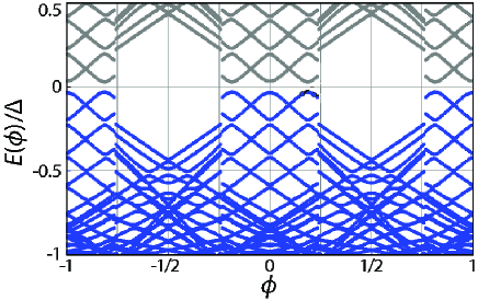
Figure 10: Energy spectrum for a $d$-wave superconductor on a square frame. The eigenenergies in the gap region are shown for a square 40$\times$40 loop with a 14$\times$14 hole and pair interaction $V_{1}=0.3t$ as a function of flux $\phi$ (in units of $\Phi_{0}$). The energies are given in units of the superconducting order parameter $\Delta$ at $\phi=0$ ($\Delta\approx 0.22t$). The superconducting condensate consists of the states below $E_{\rm F}=0$. Reconstruction of the condensate takes place near $\phi=\pm(n+1)/2$, where the eigenenergies jump abruptly (after Ref. loder:08 .

To assess the $E(\phi)$ and the current $J(\phi)$, the evolution of the eigenenergies with magnetic flux has to be calculated first. The eigenstates with energies below $E_{\rm F}$ form the ground-state condensate (Fig. 10). Here we discuss only flux values $\phi$ between 0 and $1/2$, because all quantities are either symmetric or antisymmetric with respect to flux reversal $\phi\rightarrow-\phi$. The spectrum for a square frame with $N=40$ and $L=14$ is shown in Fig. 10 for half filling, i.e., $\mu=0$. Because the number of lattice sites on straight paths around the hole is a multiple of four in a square frame, the spectrum is almost identical to the one for a cylinder with an even number of lattice sites and with the same number $N-L=26$ of transverse channels (compare to Fig. 6 in Ref. loder:09 ). For the square frame, the energy levels do not actually cross $E_{\rm F}$, because the lack of rotational symmetry leads to hybridization of the levels and level repulsion. Nevertheless, the same clearly distinct flux regimes are found: the flux intervals between 0 and $1/4$ and from $1/4$ to $1/2$ (in units of $\Phi_{0}$).

Up to $\phi\simeq 1/4$ the current $J(\phi)$ generates a magnetic field which tends to reduce the applied field by a continuous shift of the eigenenergies in the condensate. At $\phi=0$, pairs of states with opposite circulation compensate their respective currents, thus $J=0$. The well separated states at $\phi=0$ in Fig. 10 are the states in the vicinity of the nodes of the $d$-wave superconductor. Away from $E_{\rm F}$, the density of states increases towards the states near the maximum energy gap $\Delta$ that provide most of the condensation energy. For $\phi>0$, the energy of the states with orbital magnetic moment anti-parallel (parallel) to the magnetic field is increased (decreased). Correspondingly the supercurrent, which is carried by these states, depends on the details of level crossings and avoidings. The main contribution to the supercurrent arises from the occupied levels closest to $E_{\rm F}$, because the contributions from the lower-lying states tend to cancel in adjacent pairs.

As the highest occupied state shifts with increasing flux to lower energies, the current in the square loop first increases for small $\phi$ (Fig. 11), then decreases when the highest occupied level with an orbital moment opposite to the applied magnetic field starts to dominate. With increasing flux this state approaches $E_{\rm F}$. A current-carrying state in the vicinity of the nodes is replaced upon a slight increase of $\phi$ by a state of opposite current direction. The states of the condensate are thereby continuously changing near the extrapolated crossing points. As a consequence, the energy “parabola” centered at zero flux is different from the ground-state energy parabola centered at $\phi=1/2$ [Fig. 11 (a)]. The deviation from a parabolic shape near zero flux is due to the evolution of the near-nodal states; the vertical offset of the energy minima at $\phi=n$ results mostly from the flux dependence of the states near the maximum value of the anisotropic gap.

For flux values near $\phi=1/4$ the condensate reconstructs. The superconducting state beyond $1/4$ belongs to the class of wave functions introduced by Byers and Yang Byers in which, for a circular geometry, each pair acquires a center-of-mass angular momentum $\hbar$ schrieffer . Remarkably, in the flux interval from near $1/4$ to $1/2$, a full energy gap exists also for $d$-wave superconductors (Fig. 10). Here the circulating current enhances the magnetic field; the paramagnetic orbital moment of the current is parallel to the field. The resulting energy gain is responsible for the field-induced energy gap. This reconstruction of the condensate is the origin of the $\Phi_{0}$ periodicity in energy and current.

These calculations show that a $d$-wave superconducting loop in a square geometry has almost identical properties to a flux threaded cylinder. This is remarkable, because on a closed path in the square frame, the phase of the $d$-wave order parameter $\Delta^{d}_{i}$ rotates by $2\pi$, whereas in the cylinder, the order parameter rotates with the lattice. Therefore, while changes in the geometry and the number of transverse channels modify the spectrum and the $J(\phi)$ characteristics in detail, they do not eliminate the $\Phi_{0}$ periodic component. The reduction of the symmetry, here to the four-fold rotational symmetry of the square frame, stabilizes the spectrum compared to the cylinder geometry.

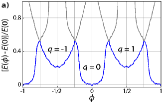
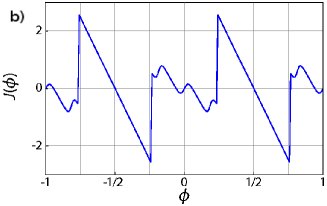
Figure 11: Flux dependence of energy and current for the square frame. Energy $[E(\phi)-E(0)]/E(0)$ (a) and circulating current $J(\phi)$ (b) for a square 40$\times$40 loop with a 14$\times$14 hole and pair interaction $V_{1}=0.3t$. $J(\phi)$ is given in units of $t/\Phi_{0}=6\times 10^{-5}{\rm A}$ for the choice of $t=250$ meV. The condensate states with even and odd winding number $q$ are clearly distinct, which is reflected, e.g., in the deformation of the $q=0$-parabola. The overall $\phi$ periodicity for $E(\phi)$ and $J(\phi)$ is $\Phi_{0}$ (from Ref. loder:08 ).

IV Flux periodicity of Josephson junctions

All energy levels are Doppler shifted in current carrying systems, not only in flux threaded loops but also in wires or at the surface of bulk superconductors. In the latter systems, the phase gradient of the superconducting order parameter typically does not reach the value necessary to drive the superconductor into a finite-momentum pairing state with $q\neq 0$, which is why the influence of finite momentum pairing on the flux periodicity has not been discussed in the literature until recently. An exception are systems with strong inhomogeneities of the order parameter, which act as Josephon junctions. The phase gradient accumulates at the junctions and they behave periodically with the phase gradient, as described by the Josephson relation. From what has been discussed for the flux periodicity in multiply connected geometries, it appears natural that the Doppler shift of nodal states might also influence the periodicity of Josephson junctions.

A Josephson junction is intrinsically a more complicated system than a superconducting loop. Several parameters are needed to characterize the junction as well as the superconducting states on each side of the junction. Most junctions can be classified either as transparent or as tunnel junctions, regardless whether they consist of a geometrical constriction, a potential barrier, or a normal metal bridge. This classification is closely related to the Doppler shift of single energy levels in the system, as will be explained below. In the following we will therefore discuss the Josephson relations in both the tunneling and the transparent regimes.

IV.1 Current-phase relation

The current-phase relation, which expresses the supercurrent $J$ over a Josephson junction as a function of the phase difference $\delta\varphi$ of the order parameters on both sides of the junction is:

$$J=J_{\rm c}\sin(\delta\varphi).$$ (46)

$J_{\rm c}$ is the critical current over the junction, above which the zero voltage state breaks down. This relation was predicted by Josephson in 1962 josephson and can be directly derived from a Ginzburg-Landau description tinkham . For transparent junctions, $\sin(\delta\varphi)$ in Eq. (46) distorts into a saw-tooth pattern similar to the current-flux relation in superconducting loops golubov:04 . It is crucial to realize that the phase gradient of the order parameter is twice that of the superconducting wave function. If the phase difference of the order parameter on both sides of the junction is $\delta\varphi$, then the phase difference of the wave function is $\delta\varphi/2$. Because the wave function of the system has to be $2\pi$-periodic, the periodicity of the energy spectrum and the order parameter of a finite system is $4\pi$. The current contributions from all energy levels add up to a $2\pi$ periodic supercurrent only in the thermodynamic limit. In this section we analyze whether the Doppler shift of the energy levels leads to the same doubling of the periodicity in $\delta\varphi$ of a junction as it does for the flux periodicity of loops. While for the tunneling regime we rely on a simple linear-junction model, we will analyze transparent junctions by inserting a Josephson junction into a square frame. This has the advantage of a remarkable stability of the energy spectrum against the insertion of impurities and lattice defects, as will be seen in Sec. IV.1.2.

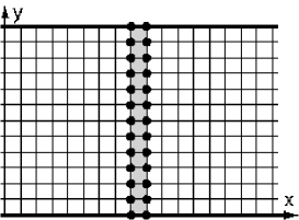
Figure 12: To model a Josephson junction we choose a discrete square lattice with $N$ sites in $x$-direction, and $M$ sites in $y$-direction. The junction itself is modeled by one or two lines of potential scatterers (black points) each with a repulsive potential $U>0$.

IV.1.1 Tunnel junctions

A simple model of a tunnel junction is a square lattice with $N$ sites in $x$-direction and $M$ sites and periodic boundary conditions in $y$-direction. The junction is modeled in the tunneling regime by one or two lines of potential scatterers with a repulsive potential $U>4t$ (Fig. 12). In the absence of a magnetic field, this system is homogeneous in $y$-direction, and the Fourier transformation with respect to the $y$-coordinate will allow the diagonalization of larger systems andersen .

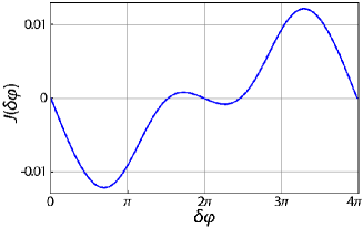
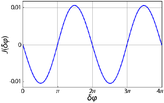
Figure 13: Current-phase relation calculated for Josephson junctions in the tunneling regime. Left panel: $N=18$, $M=12$, $V_{1}=0.3t$, and $U=4.5t$. The $\sin(\delta\varphi)$ relation is considerably deformed, which is typical for narrow junctions with very few channels. Right panel: $N=20$, $M=200$, $V_{1}=t$, and $U=5t$. This junction has a sufficiently many channels to exhibit the known current-phase relation. The overall sign depends on the choice of the sign in the phase factor of the hopping matrix elements.

The Bogoliubov – de Gennes equations are slightly modified in this case: the eigenvalue equation (40) for nearest-neighbor interaction is now defined through the relations

$$\hat{t}u_{n_{i_{x}k_{y}}}=\sum_{j_{x}}t_{ij}u_{n_{j_{x}k_{y}}}+(\epsilon_{k_{y}}+U_{i_{x}})u_{n_{i_{x}k_{y}}}\hskip 8.5359pt,\hskip 8.5359pt\\ \hat{\Delta}v_{n_{i_{x}k_{y}}}=\sum_{j_{x}}\Delta_{ij}v_{n_{j_{x},k_{y}}}+\Delta_{k_{y}}v_{n_{i_{x}k_{y}}},$$ (47)

where $\epsilon_{k_{y}}=-2t\cos(k_{y})-\mu$ and $\Delta_{k_{y}}=\Delta_{y}\cos(k_{y})$. The indices of the eigenvectors ${\bf u}_{n}$ and ${\bf v}_{n}$ are the $x$-coordinate of the site and the wave number $k_{y}$ in $y$-direction. The corresponding self-consistency equations are

$$\Delta_{ij}=\frac{V_{1}}{2}\sum_{n,k_{y}}\left[u_{n_{i_{x}k_{y}}}v^{*}_{n_{j_{x}k_{y}}}+u_{n_{j_{x}k_{y}}}v^{*}_{n_{i_{x}k_{y}}}\right]\tanh\left(\frac{E_{n}(k_{y})}{2k_{\rm B}T}\right),$$ (48)

if $j=i\pm\hat{x}$, and if the bonds are along the $y$ direction

$$\Delta_{y}=V_{1}\sum_{n,k_{y}}u_{n_{i_{x}k_{y}}}v^{*}_{n_{i_{x}k_{y}}}\cos(k_{y})\tanh\left(\frac{E_{n}(k_{y})}{2k_{\rm B}T}\right).$$ (49)

The self-consistency equation for the $s$-wave order parameter $\Delta_{i}$ with on-site interaction is analogous to (49), but without the factor $\cos(k_{y})$.

To induce a finite phase gradient of the order parameter and a supercurrent, we introduce a “phase jump” $\delta\varphi$ in the matrix elements $t_{ij}$ for hopping from $i_{x}=N-1$ back to $i_{x}=0$, and a jump $-\delta\varphi$ for the corresponding hopping in the opposite direction. An alternative, but physically equivalent choice for the phase of $t_{ij}$ is a constant phase factor $e^{i\varphi_{ij}}$ with $\varphi_{ij}=\delta\varphi/N$ for all hopping processes along the $x$-direction, which is mathematically identical to a cylinder threaded by a flux $\Phi=(hc/e)\,\phi$ with $2\pi\phi=\delta\varphi/2$. In the fully transparent case with $U=0$, this leads to a homogeneous phase gradient of $\Delta^{d}_{i}=(\Delta_{i,i+\hat{x}}+\Delta_{i,i-\hat{x}})/2+\Delta_{y}$ (or $\Delta_{i}$, respectively), whereas far in the tunneling regime for $U>4t$, the phase of the order parameter drops only across the junction. The current across the junction is calculated as in Eq. (45). The results for two typical situations are shown in Fig. 13. The left panel displays the current-phase relation of a narrow Josephson junction with a width of $M=12$ sites. The usual current-phase relation is considerably deformed in this case, as is typical for junctions with very few channels golubov:04 . The exact form of the current-phase relation is characteristic for each junction; it depends on the structure of the energy spectrum, which changes strongly upon increasing or decreasing the system size or adding impurities. For increasing $M$, the current-phase relation approaches (46), as the level spacing becomes negligible. This is the regime of wide junctions, shown in Fig. 13 (right panel), which is well described by the Ginzburg-Landau approach.

Figure 14: The top 14 energy levels below $E_{F}$ calculated for a linear Josephson juntion with $N=18$, $M=12$ and $V_{1}=0.6t$ as a function of the repulsive potential $U$ on the junction.

Our numerical analysis shows that the Josephson relation (46) describes wide junctions in the tunneling regime very well; a doubling of the period is not observed, even for $d$-wave superconductors with small antinodal energy gap. The reason for this is twofold: (1) Along with the suppression of the critical current $J_{\rm c}$ across the junction, the Doppler shift decreases strongly with increasing repulsive potential $U$. In the tunneling regime ($U>4t$), $J_{\rm c}$ decreases by a factor $>10^{3}$. Consequently no energy levels (or negligibly few in very large systems) approach $E_{\rm F}$ as a function of $\delta\varphi$ and the effects related to a reversal of single particle currents are absent. (2) For tunnel junctions, the thermodynamic Ginzburg-Landau limit is reached also for $d$-wave superconductors, if the density of states close to $E_{\rm F}$ becomes quasi-continuous, in contrast to the flux threaded loop. The deformation of the current-phase relation in narrow tunnel junctions is generically not due to levels reaching $E_{\rm F}$. The deformation is induced, if the total current is carried by very few states, each with a period of $4\pi$. The $2\pi$-asymmetric terms do not cancel and the critical current is $4\pi$-periodic.

IV.1.2 Transparent junctions

Transparent junctions are more involved than tunnel junctions. One reason for their complexity is the strong coupling of the superconducting states on both sides of the junction,which does not allow to choose the phases of the corresponding order parameters independently. Consequently the phase difference $\delta\varphi$ is not an adequate variable for describing the current across the junction. Another reason is that the energy spectrum in a linear junction of the type shown in Fig. 12 changes strongly upon changing microscopic details of the system, such as the strength of the repulsive potential $U$ on the impurity sites in this case. This is illustrated vividly by Fig. 14 showing the evolution of the highest occupied energy levels with increasing $U$.

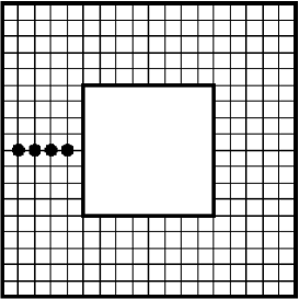
Figure 15: For the description of transparent junctions, we choose the square-frame geometry and model the junction with potential scatterers arranged on a line crossing one side on the frame (black points). The current is driven by a magnetic flux threading the frame.

These problems can be resolved by using a square-frame geometry as in Sec. III.2. Here the Josephson junction is modeled by adding potential scatterers on a line as shown in Fig. 15, and the current is driven by a magnetic flux $\phi$ threading the frame. For a tunnel junction, this would induce a phase jump of $4\pi\phi$ in the order parameter aross the junction and thus a $\sin(4\pi\phi)$ current-flux relation. In transparent junctions, the jump is smaller and vanishes in a clean frame. For this topology the magnetic flux $\Phi=\phi\cdot hc/e$ is related to the phase variation of the order parameter $\delta\varphi$ by $2\pi\phi=\delta\varphi/2$.

For sufficiently large $U$, say $U=100t$, these impurities act as a geometrical constriction. Figure 16 shows explicitly that the spectrum of a square frame remains qualitatively invariant upon inserting a small number of impurities, even sufficiently strong to block the current over the impurity site completely. Figures 16 (b) and (c) show the spectra versus $\phi$ for two and four impurities for a $20\times 20$ square frame with a $8\times 8$ square hole. In the presence of impurities, bound states arise at $E_{\rm F}$ in a $d$-wave superconductor zhu:00 ; franz:96 , which are nearly flux independent. These bound states are easily identified in Figs. 16 (a) and (b) near the Fermi energy. Otherwise, the spectrum in Fig. 16 (b) is very similar to that of the clean frame discussed in Sec. III.2 (Fig. 10). Clearly visible is the discontinuity of the spectrum where the condensate reconstructs to a superconducting state with different winding number $q$. The relevance of $q$ is a characteristic property of transparency and directly connected to a discontinuity of the supercurrent (see Fig. 16 (a) for one and two impurities).

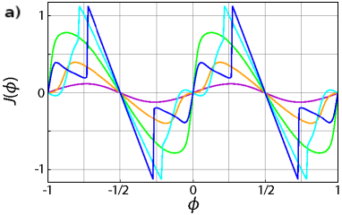
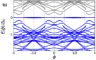
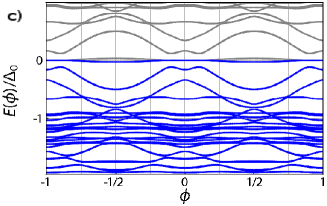
Figure 16: Supercurrent $J(\phi)$ and energy spectrum $E(\phi)$ of a $20\times 20$ square frame with an $8\times 8$ hole containing a Josephson junction. The width of the arms for the frame is six sites. The impurity potential is $U=100t$. (a) $J(\phi)$ for one (blue), two (turquoise), three (green), four (orange), and five (purple) impurity sites. Energy spectrum for (b) two and (c) four impurity sites.

For three to five impurities, the supercurrent is continuous, as is the spectrum shown in Fig. 16 (c) for four impurities. Nevertheless, the typical features of the square-frame spectrum are still present, in particular the gap in the odd flux regimes and one energy level approaching $E_{\rm F}$ in the even $q$ regime. This level causes the wiggle in the supercurrent around $\phi=0$; its slope and that of a few others remain almost as steep as in a clean frame, which indicates the existence of channels with free current flow. The Doppler shift of nodal states is therefore not negligible in the calculation of the supercurrent across transparent Josephson junctions, and it may cause appreciable deviations from the $\sin(4\pi\phi)$ current-flux relation even in the case of wide junctions. The $\sin(4\pi\phi)$ is expected for the thermodynamic Ginzburg-Landau limit.

Finally we note that for five impurities, only one channel through the junction remains, which is almost blocked by the bound state. Thus the spectrum becomes nearly flux independent, leading to a junction in the tunneling regime. However, the supercurrent does not follow the expected $\sin(4\pi\phi)$ but rather a $\sin(2\pi\phi)$ current-phase relation. This is due to the point-contact like character of the junction and the extreme limit of the deformation of the current-flux relation as shown in Fig. 13 – similar to the left panel, however with $J(\delta\varphi)\sim-\sin(\delta\varphi/2)$.

IV.2 Field-threaded junctions

A magnetic field threading a Josephson junction modifies the phase difference of the order parameters of the superconductors on both sides and thus alters the supercurrent. This behavior is well understood on the basis of the Ginzburg-Landau approach. The current-flux relation of a linear junction that is homogeneous in $y$-direction has the shape of a Fraunhofer diffraction pattern tinkham , although it deviates from the Fraunhofer form for all other junction geometries. Despite these deviations it preserves the characteristic flux periodicity of $\Phi_{0}/2$ for conventional Josephson junctions. The magnetic field dependent critical current of Josephson junctions is therefore another key property where the Doppler shift might cause a doubling of the flux period.

Here we use again the linear junction model of Sec. IV.1.1 and fix the phase difference to $\delta\varphi=\pi/2$, for which the absolute value of the current across the junction in the tunneling regime is largest. In order to introduce a magnetic field threading the junction, we construct the junction from single plaquettes with potential scatterers on each of its sites. All plaquette $l$ which belong to the junction are threaded by a magnetic flux $\phi^{l}$, generating Peierls phase factors $\varphi^{l}_{ij}$. We restrict our discussion to a homogeneous field distribution inside the junction, $\phi^{l}=\phi$ for all $l$, and the repulsive potential on the respective sites is $U$. In the presence of a magnetic field, the system is not homogeneous in $y$-direction, and we have to diagonalize it in real space. This restricts the maximum system size for our analysis.

IV.2.1 Current-flux relation of tunnel junctions

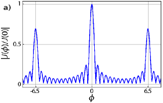
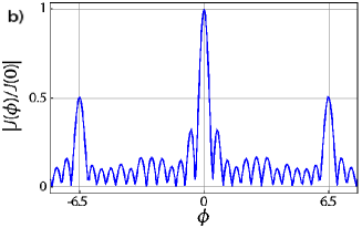
Figure 17: Absolute value of the maximum current flowing across a tunnel junction versus the total applied magnetic flux $\phi$ (in units of $hc/e$) obtained from the Bogoliubov – de Gennes equations solved on a lattice with $N=16$, $M=14$, $U=5t$, and $\delta\varphi=\pi/2$ in units of $J(0)$. (a) $s$-wave pairing with $V_{0}=t$. (b) $d$-wave pairing with $V_{1}=0.7t$. Here $\phi$ is the flux within the junction.

The simplest model of a field-threaded Josephson junction consists of two lines of impurity sites as used in Sec. IV.1.1 (Fig. 12). The current-flux relation of such a junction as obtained from the Bogoliubov – de Gennes equations is shown in Fig. 17 for $s$- and $d$-wave junctions with a length of 14 sites and thus 13 plaquettes. Upon first glance, the current-flux relation of the $s$-wave junction [Fig. 17 (a)] appears to be similar to the Fraunhofer pattern known from the Ginzburg-Landau approach for linear Josephson junctions tinkham , as does the current-flux relation for the $d$-wave junction [Fig. 17 (b)]. The characteristics are a central peak around $\phi=0$ with width $\Phi_{0}$ and side peaks of decreasing height with width $\Phi_{0}/2$. They display the expected global periodicity of $13\Phi_{0}$, enforced by gauge invariance, if each plaquette is threaded by an integer multiple of $\Phi_{0}$. On closer inspection of Fig. 17 (a) one finds that the $s$-wave junction has one maximum surplus in one period of $13\Phi_{0}$, whereas the $d$-wave junction has not. The width of the peaks in Fig. 17 (a) is therefore slightly smaller than the expected value $\Phi_{0}$. In the following, we explain this effect jointly with an investigation of the current-flux relation of inhomogeneous junctions by analyzing the Ginzburg-Landau approach for a lattice model.

We consider a two-dimensional superconductor which is divided by a thin, quasi one-dimensional Josephson junction of width $d$ oriented along the $y$-direction with $d\ll\lambda$, such that screening currents are negligible; $\lambda$ is the London penetration depth. If the junction is threaded by a constant magnetic field $B_{z}(x,y)=B_{z}$, the supercurrent across the junction derived from the Ginzburg-Landau equations is

$$J=\int{\rm d}y\,j_{\rm c}(y)\sin(ky),$$ (50)

where $k=\pi B_{z}d/\Phi_{0}$. The critical current density $j_{\rm c}(y)$ is controlled by the microscopic structure of the junction. If $j_{\rm c}(y)$ is constant, one obtains the well known Fraunhofer pattern

$$\left|\frac{J(\Phi)}{J(0)}\right|=\left|\frac{\sin(\pi\Phi/\Phi_{0})}{\pi\Phi/\Phi_{0}}\right|$$ (51)

for the current across the junction; $\Phi$ is the total magnetic flux through the area of the junction.

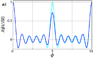
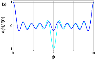
Figure 18: Current-flux relation of a Josephson junction as in Fig. 17 but with $M=11$ (10 plaquettes) as obtained from the Bogoliubov – de Gennes equations (blue) and from the discrete Ginzburg-Landau approach (turquoise). (a) $s$-wave pairing: The peaks at $\phi=(M-1)/2$ and $\phi=0$ have the same sign. (b) $d$-wave pairing: The peaks at $\phi=(M-1)/2$ and $\phi=0$ have the opposite sign.

On a discrete square lattice with $M$ lattice sites in $y$-direction and an order parameter defined on the lattice sites ($s$-wave), Eq. (50) becomes

$$J=\sum_{i=1}^{M}j_{{\rm c},i}\sin(ky_{i}).$$ (52)

If $j_{{\rm c},i}$ is equal for all $i$, one obtains a flux dependence similar to the Fraunhofer pattern:

$$\frac{J(\phi)}{J(0)}=\sum_{i=1}^{M}\sin(ky_{i})/(M+1)=\frac{\sin\left(k(M+1)/M\right)}{(M+1)\sin\left(k/M\right)}.$$ (53)

This formula reproduces the flux dependence of the supercurrent as obtained from the Bogoliubov – de Gennes equations (shown in Fig. 18), apart from slight deviations in the amplitude around the central peak at $\phi=(M-1)/2$. It explains naturally the deviation from the $\Phi_{0}/2$ periodicity: it is an effect of discreteness, caused by the fact that the number of lattice sites in $y$-direction exceeds the number of plaquettes by one.

¿From what has been explained for an $s$-wave junction, we construct a simple Ginzburg-Landau analogon for a $d$-wave junction. In a $d$-wave superconductor, the order parameter is defined on the bonds between two neighboring lattice sites, and we therefore define the corresponding supercurrent as

$$J=\sum_{i=1}^{M-1}j_{{\rm c},i}\sin(k(y_{i}+1/2)).$$ (54)

For a constant $j_{{\rm c},i}$ we obtain

$$\frac{J(\phi)}{J(0)}=\sum_{i=1}^{M-1}\sin(k(y_{i}+1/2))/M=\frac{\sin\left(k\right)}{M\sin\left(k/M\right)},$$ (55)

which indeed reproduces the $\Phi_{0}/2$ periodic Fraunhofer pattern obtained from the Bogoliubov – de Gennes equations with nearest-neighbor pairing. The deviations in the amplitude are larger than for the $s$-wave junction telling that the $d$-wave junctions fulfill the Ginzburg-Landau conditions not as well as the $s$-wave junction.

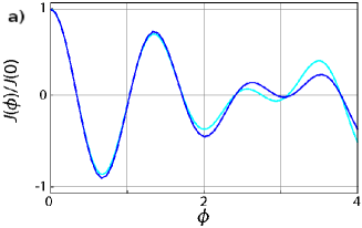
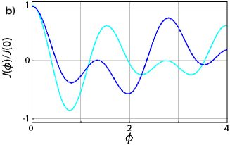
Figure 19: Current-flux relation calculated for a Josephson junction with $M=11$ and an inhomogeneous impurity distribution. Top panel: The gray plaquettes in the profile of the junction have a scattering potential $U=100t$, while the white plaquettes have $U=2t$, thus leaving two transparent channels through which almost the entire current flows. Blue: Bogoliubov – de Gennes equations and turquoise: Ginzburg-Landau model for (a) $s$-wave pairing and (b) $d$-wave pairing.

The Ginzburg-Landau formulae (52) and (54) are suitable also to calculate the supercurrent flowing across junctions with an inhomogeneous impurity distribution. It is instructive to compare also in this case the supercurrent to results obtained from the Bogoliubov – de Gennes equations. Figure 19 shows such a comparison for a junction with $M=11$ and current flowing only through the two “gaps” between the white plaquettes in the top panel of Fig. 19. In the microscopic model, this is achieved by setting strong repulsive potentials $U=100t$ on the sites of the gray plaquettes and a small potential $U=2t$ on the white plaquettes. In the Ginzburg-Landau approach, we set $j_{{\rm c},i}=0$ except for the two transparent channels. This system appears to be quite far from respecting the conditions for the validity of the Ginzburg-Landau equations. Nevertheless, for the $s$-wave junction, the results obtained from the Bogoliubov – de Gennes and Ginzburg-Landau equations are remarkably close. Even for the $d$-wave junction, the simple implementation of the Ginzburg-Landau equations reproduces the same features as the Bogoliubov – de Gennes equations, in particular it has maxima for similar values, but the amplitudes of the oscillations deviate strongly.

These considerations jointly lead to the conclusion that, even for small junctions where discreteness is pronounced, we do not find any indications that the Doppler shift has an effect on the current-flux relation of Josephson junctions in the tunneling regime. The essential characteristics of the current-flux relation, especially the position of the current maxima, agree quite well with the Ginzburg-Landau approach, where these effects are not included.

IV.2.2 Current-flux relation of transparent junctions

A magnetic field threading a Josephson junction generates a supercurrent circulating around the junction, similar to a vortex in a type II superconductor, but with the complete flux confined to the junction. If the junction is sufficiently transparent, the order parameter reacts to the current loop with a phase winding as in a flux-threaded ring, with a winding number $q$ that minimizes the total energy. The superconducting state in a transparent junction is therefore characterized similarly as a loop by the quantum number $q$ related to a center-of-mass motion of the Cooper pairs and the supercurrent across the junction changes sign when the condensate reconstructs to another $q$. Remarkably, if the transparency is reduced, the discontinuities vanish smoothly, the current-flux relation of the superconducting state with fixed $q$ becomes periodic in $\phi$, and in the tunneling regime, all states with different $q$ become equivalent. This behavior is illustrated in Fig. 20, which shows $E(\phi)$, $J(\phi)$, and the spectrum for a uniform junction with nearest-neighbor pairing and $U=2t$. The total energy consists of a series of parabolae, which correspond to different phase winding numbers. The kinks in $E(\phi)$ and in the flux dependence of the spectrum are sharp for small values of $\phi$, but the finite repulsion on the junction smoothens the discontinuities in the supercurrent. Although the Doppler shift of the energy levels is not strongly pronounced in Fig. 20, the physical phenomena typical for multiply connected geometries govern the field dependence of the supercurrent across a Josephson junction, if its transparency is sufficiently high.

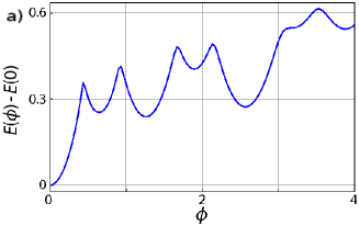
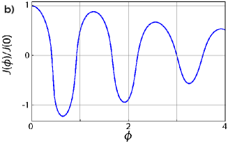
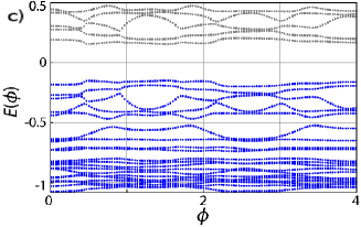
Figure 20: Characteristics of a transparent junction as obtained from the Bogoliubov – de Gennes equations in a system with $N=14$ and $M=12$ and a homogeneous impurity distribution with repulsive potential $U=2t$. (a) The total energy, (b) the Josephson current, and (c) the energy spectrum of the system versus the external flux through the junction.

V Conclusions

For unconventional nodal superconductors we established within a momentum-space formulation for superconducting loops that $hc/e$ oscillations are present in the flux dependence of the ground state. The calculations in momentum space were restricted to rotationally symmetric systems like a cylinder, the energy spectrum of which depends sensitively on microscopic details. In Sec. III.2 we have provided an analysis of the flux periodicity in a square frame with $d$-wave pairing symmetry analogous to the cylinder geometry of Sec. II with remarkably similar results. Nevertheless, the real-space calculations contributed to the understanding of the flux periodicity. We verified that the characteristic flux dependence of the $d$-wave energy spectrum does not depend on the geometry or the absence of impurities.

Within the real-space formulation, we constructed and analyzed more complex systems, in particular we investigated the periodicity of Josephson junctions. The idea that the Doppler shift drives energy levels through the Fermi energy in junctions between $d$-wave superconductors, and thereby doubles the periodicity of the current-phase relation, seemed natural, but the physics turned out to be more subtle. Narrow junctions with only a few channels always display a period in the phase difference of $4\pi$, even for $s$-wave superconductors, and the Doppler shift in tunnel junctions is too small to influence the current-phase relation. Only for transparent junctions does the Doppler shift become important; in this regime the supercurrent across a Josephson junction behaves similar to the persistent supercurrent in a loop. These observations are also valid for the current-flux relation of field-threaded junctions. The microscopic theory excellently reproduced the results from the Ginzburg-Landau description of Josephson junctions in the tunneling regime, even for nanoscopically small systems with $d$-wave pairing.

We thank R. Frésard, S. Graser, C. Schneider, and D. Vollhardt for insightful discussions and J. Mannhart for valuable contributions. This work was supported by the Deutsche Forschungsgemeinschaft through SFB 484 and TRR 80.

References

- (1) W. Ehrenberg, R. E. Siday, Proc. Phys. Soc. B 62, 8 (1949)
- (2) Y. Aharonov, D. Bohm, Phys. Rev. 115, 485 (1959)
- (3) F. London, Superfluids, John Wiley & Sons, New York (1950)
- (4) J. Bardeen, L. N. Cooper, J. R. Schrieffer, Phys. Rev. 108, 1175 (1957)
- (5) R. Doll, M. Näbauer, Phys. Rev. Lett. 7, 51 (1961)
- (6) B. S. Deaver, W. M. Fairbank, Phys. Rev. Lett. 7, 43 (1961)
- (7) A. A. Abrikosov, Soviet Physics – JETP 5, 1174 (1957)
- (8) U. Essmann, H. Träuble,. Phys. Lett. A 24, 526 (1967)
- (9) L. Onsager, Phys. Rev. Lett. 7, 50 (1961)
- (10) N. Byers, C. N. Yang, Phys. Rev. Lett. 7, 46 (1961)
- (11) W. Brenig, Phys. Rev. Lett. 7, 337 (1961)
- (12) J. R. Schrieffer, Theory of Superconductivity, Addison Wesley (1964), chapter 8
- (13) F. Loder, A. P. Kampf, T. Kopp, J. Mannhart, C. Schneider, Yu. S. Barash, Nature Phys. 4, 112 (2008)
- (14) F. Loder, A. P. Kampf, T. Kopp, Phys. Rev. B 78, 174526 (2008)
- (15) V. Juričić, I. F. Herbut, Z. Tešanović, Phys. Rev. Lett. 100, 187006 (2008)
- (16) Yu. S. Barash, Phys. Rev. Lett. 100, 177003 (2008)
- (17) S. Washburn, R. A. Webb, Rep. Prog. Phys. 55, 1311 (1992)
- (18) R. M. Fye, M. J. Martins, D. J. Scalapino, J. Wagner, W. Hanke, Phys. Rev. B 44, 6909 (1991); Phys. Rev. B 45, 7311 (1992)
- (19) S. V. Sharov, A. D. Zaikin, Phys. Rev. B 71, 014518 (2005)
- (20) X. Waintal, G. Fleury, K. Kazymyrenko, M. Houzet, P. Schmitteckert, D. Weinmann, Phys. Rev. Lett. 101, 106804 (2008)
- (21) V. P. Mineev, K. V. Samokhin, Introduction to Unconventional Superconductivity, Gordon and Breach Science Publishers (1999), chapters 5, 8, and 17
- (22) F. Loder, A. P. Kampf, T. Kopp, Phys. Rev. B 81,020511(R) (2010)
- (23) K. Czajka, M. M. Maśka, M. Mierzejewski, Z. Śledź, Phys. Rev. B 72, 035320 (2005)
- (24) D. J. Scalapino, S. R. White, S. Zhang, Phys. Rev. B 47, 7995 (1993)
- (25) C. J. Pethick, H. Smith, Annals of Physics 119, 133 (1979)
- (26) M. Tinkham, Superconductivity, McGraw-Hill Internation Editions (1996), chapters 3 and 6
- (27) F. von Oppen, E. K. Riedel, Phys. Rev. B 46, 3203 (1992)
- (28) I. Khavkine, H.-Y. Kee, K. Maki Phys. Rev. B. 70, 184521 (2004)
- (29) W. A. Little, R. D. Parks, Phys. Rev. Lett. 9, 9 (1962)
- (30) R. D. Parks, W. A. Little, Phys. Rev. 133, A97 (1964)
- (31) P. I. Soininen, C. Kallin, A. J. Berlinsky, Phys. Rev. B 50, 13883 (1994)
- (32) Y. Wang, A. H. MacDonald, Phys. Rev. B 55, R3876 (1995)
- (33) J.-X. Zhu, T. K. Lee, C. S. Ting, C.-R. Hu, Phys. Rev. B 61, 8667 (2000)
- (34) J.-X. Zhu, C. S. Ting, Phys. Rev. Lett. 87, 147002 (2001)
- (35) A. Ghosal, C. Kallin, A. J.Berlinsky, Phys. Rev. B 66, 214502 (2002)
- (36) Y. Chen, Z. D. Wang, C. S. Ting, Phys. Rev. B 67, 220501 (2003)
- (37) M. Franz, C. Kallin, A. J. Berlinsky, Phys. Rev. B 54, R6897 (1996)
- (38) P. F. Bagwell, Phys. Rev. B 49, 6841 (1994)
- (39) F. Loder, A. P. Kampf, T. Kopp, J. Mannhart, New J. Phys. 11, 075005 (2009)
- (40) D. B. Josephson, Phys. Lett. 1, 251 (1962)
- (41) A. A. Golubov, M. Y. Kupriyanov, E. Il’ichev, Rev. Mod Phys. 76, 411 (2004)
- (42) P. G. de Gennes, Superconductivity of Metals and Alloys, Addison Wesley (1966), chapter 5
- (43) B. M. Andersen, I. V. Bobkova, P. J. Hirschfeld, Yu. S. Barash, Phys. Rev. B 72, 184510 (2005); Phys. Rev. Lett 96, 117005 (2006)
- (44) J. Cayssol, T. Kontos, G. Montambaux, Phys. Rev. B 67, 184508 (2003)