Computation of ground-state properties of strongly correlated many-body systems by a two-subsystem ground-state approximation

Abstract

We present a new approach to compute low lying eigenvalues and corresponding eigenvectors for strongly correlated many-body systems. The method was inspired by the so-called Automated Multilevel Sub-structuring Method (AMLS). Originally, it relies on subdividing the physical space into several regions. In these sub-systems the eigenproblem is solved, and the regions are combined in an adequate way. We developed a method to partition the state space of a many-particle system in order to apply similar operations on the partitions. The tensorial structure of the Hamiltonian of many-body systems make them even more suitable for this approach.

The method allows to break down the complexity of large many-body systems to the complexity of two spatial sub-systems having half the geometric size. Considering the exponential size of the Hilbert space with respect to the geometric size this represents a huge advantage. In this work, we present some benchmark computations for the method applied to the one-band Hubbard model.

1 Introduction

In modern solid-state physics strongly correlated many-body systems play an increasingly important role, as e.g. in the case of the high temperature superconductors, the manganites and vanadates, and more recently also in light-matter- and ion trap quantum simulators. The numerical problem of addressing strong correlations leads to eigenvalue problems of matrices whose size depend exponentially on the geometric size and the particle number.

Several methods have been introduced to solve problems of this kind. Quantum Monte-Carlo (QMC, [1]) is a powerful method to deal with finite-temperature systems, where large system sizes can be reached. On the downside, many system configurations cannot be addressed efficiently due to the so-called sign-problem [2]. Another powerful method is the Density Matrix Renormalization Group (DMRG, [3]) which allows to solve for ground-state properties of comparatively large-scale electronic structures. Its disadvantages include the lack of possibility of treating problems apart from 1D or pseudo-1D problems. Newer methods like the Variational Cluster Perturbation Theory (VCPT) also deliver promising results.

For this work we followed a new approach to break down the numerical complexity of such systems. Rather than starting from a physical point of view we let ourselves be inspired by other fields of numerical simulations, which also deal with large-scale eigenvalue calculations. The Automated Multilevel Sub-structuring Method (AMLS, [4, 5]) e.g. for linear elastodynamics relies on partitioning the physical space into smaller pieces wherein the eigenproblem is solved as a starting point for the calculation of the full system eigenvalues. We refer to our approach as Two Sub-system Ground-state Approximation (TSGSA).

2 Partitioning the occupation number state space

In second quantization the ab initio and approximation free form of the Hamiltonian for the electronic degrees of freedom reads

$$\hat{H} =\sum_{\nu,\nu^{\prime}}t_{\nu\nu^{\prime}}\hat{a}^{\dagger}_{\nu}\hat{a}^{\phantom{\dagger}}_{\nu^{\prime}}+\sum_{\nu,\nu^{\prime},\mu,\mu^{\prime}}V_{\nu\nu^{\prime}\mu\mu^{\prime}}\hat{a}^{\dagger}_{\nu}\hat{a}^{\dagger}_{\mu}\hat{a}^{\phantom{\dagger}}_{\nu^{\prime}}\hat{a}^{\phantom{\dagger}}_{\mu^{\prime}}\;,$$

where the operator $\hat{a}^{\dagger}_{\nu}$ ($\hat{a}^{\phantom{\dagger}}_{\nu}$) creates (annihilates) a fermion in orbital $\phi_{\nu}$. The quantity $\nu=(i,\alpha,\sigma)$ represents a combined index including the site- (unit cell-) index $i$, the index $\alpha$ of the basis function to describe the orbitals of the various atoms within a unit cell, and the spin $\sigma$. $t$ and $V$ are the corresponding matrix elements for the single particle part (hopping) and the interaction, respectively. A suitable basis for the many-body problem in second quantization is the occupation basis $|\{n_{\nu}\}\rangle$, where the occupation $n_{\nu}$ for fermions can only be 0 or 1, in accordance with the Pauli principle. There are three sources for the intricacy of a many-body problem. The first one is the number of orbital degrees of freedom per unit cell, required for a quantitatively accurate description of the band structure. The second concerns the overwhelming number of basis states for a true many-body calculation. Let $L_{r}$ be the number of unit cells and $L_{b}$ the number of orbitals within a unit cell then there are $L=L_{r}L_{b}$ different index tuples $\nu=(i,\alpha)$ for each electron spin direction. There are correspondingly $L$ occupation numbers $n_{\nu}$ which can either be 0 or 1. The number of many-body basis states to describe a system of $N_{\uparrow}$ ($N_{\downarrow}$) electrons with spin up (down) is given by the number of possibilities to distribute $N_{\uparrow}$ entries 1 and $N-N_{\uparrow}$ entries 0 among the $L$ occupation numbers and likewise for the spin down electrons. Hence the number $M$ of many-body basis states is

$$M={L\choose N_{\uparrow}}{L\choose N_{\downarrow}}\;.$$

It is needless to emphasize that a true many-body ab-initio calculation is out of reach.

In order to study the generic properties of strongly correlated many-body systems qualitatively it is, however, sufficient to reduce the number of orbital degrees of freedom to a minimum. Common many-body models include up to $L_{b}=3$ orbitals per unit cell.

But even with a strongly reduced number of orbital degrees of freedom there remains a third problem, the structure of the interaction part, which is still too complicated for an exact treatment, as well by numerical as by analytical means. There is reason to believe that the genuine many-body effects can already by described and understood when only short ranged density-density terms of the form

$$\hat{H}_{\text{int}} =\sum_{\nu\nu^{\prime}}V_{\nu\nu^{\prime}}\hat{n}_{\nu}\hat{n}_{\nu^{\prime}}\;,$$

are retained in the model. The density operator is given by $\hat{n}_{\nu}=\hat{a}^{\dagger}_{\nu}\hat{a}^{\phantom{\dagger}}$.

Though not really necessary, but in order to keep the number of parameters small, the hopping part is commonly approximated by a tight-binding form, allowing for nearest neighbor hopping only. The following extended Hubbard-model with one orbital degree of freedom per unit cell includes an on-site and a next-nearest neighbor interaction:

$$\hat{H} =-t\sum_{\langle i,j\rangle,\sigma}\hat{a}^{\dagger}_{i,\sigma}\hat{a}_{j,\sigma}+U\sum_{i}\hat{n}_{i,\uparrow}\hat{n}_{j,\downarrow}+V\sum_{\langle i,j\rangle}\hat{n}_{i}\hat{n}_{j}\;.$$

Here, we will consider the two most simple and common fermionic models, the case of spin-less fermions (only one spin-species) with nearest neighbor interaction and the Hubbard model (only on-site Coulomb interaction).

For spin-less fermions the Hamiltonian reads

$$\hat{H} =-t\sum_{\langle ij\rangle}\hat{a}^{\dagger}_{i}\hat{a}^{\phantom{dagger}}_{j}+V\sum_{\langle ij\rangle}\hat{n}_{i}\hat{n}_{j}\;,$$

where $i$ stands for the unit cells and $\langle ij\rangle$ indicates that the unit cells $i$ and $j$ are nearest neighbors.

The Hubbard Hamiltonian is given by

$$\hat{H} =-t\sum_{\langle ij\rangle,\sigma}\hat{a}^{\dagger}_{i\sigma}\hat{a}^{\phantom{dagger}}_{j\sigma}+U\sum_{i}\hat{n}_{i\uparrow}\hat{n}_{i\downarrow}\;.$$

Despite of the strong reduction in degrees of freedom, the number of many-body basis states is still very large and increases exponentially with increasing number of orbitals (sites) $L$. In the case of spin-less fermions we have $M={L\choose N}$ and for the Hubbard model, it reads as mentioned before $M={L\choose N_{\uparrow}}{L\choose N_{\downarrow}}$.

For example, a system of spin-less fermions on $L=20$ sites with $N=10$ electrons has $M=184,756$ many-body basis states, while a system of half the size, i.e. $L=10$ sites with $N=5$ has merely $M=252$. For the Hubbard model the situation is even more pronounced. Again for a half filled system with 20 sites and 10 electrons of each species, we find $M\approx 3\cdot 10^{10}$, while the half filled system on 10 sites has $M\approx 6\cdot 10^{4}$. So the numerical complexity increases by roughly $10^{6}$ if we double the geometrical size of the system.

The idea of the present paper is to exploit systematically the fact that smaller sub-systems have a significantly reduced Hilbert space.

2.1 Sectors in occupation number state space

The full Hamiltonian, be it the Hubbard or the spin-less fermion model, conserves the number of particles per spin direction $N_{\sigma}$. Therefore, the Hamilton matrix is block diagonal in the occupation number basis due to the conservation of particle numbers and we solve the eigenvalue problem for fixed number of particles $(N_{\uparrow},N_{\downarrow})$ separately. The case of the spin-less fermion model can be traced back to the Hubbard case by assuming only one spin direction. Here we restrict the discussion to an even number of lattice sites $L=2L_{h}$ and an even number of electrons per spin direction $N_{\sigma}=2N_{h,\sigma}$. Although the generalization is straightforward, it would hamper the discussion unnecessarily.

Now we split the lattice into two sub-systems $A$ and $B$ of equal size. In the approach to be discussed below, we will start from the case of completely decoupled sub-systems, i.e. all hopping and interaction effects between the two sub-systems are ignored. Consequently, the numbers of electrons per spin direction are conserved in each sub-system separately. Due to the particle number conservation in the sub-systems, the corresponding occupation number state space can be split into different sectors $(l_{\uparrow},l_{\downarrow})$, which are characterized by the number of particles per spin direction $(N_{\uparrow}=N_{h,\uparrow}+l_{\uparrow},N_{\downarrow}=N_{h,\downarrow}+l_{\downarrow})$ in the sub-systems under consideration. Here we have introduced a the quantity $l_{\sigma}$ which specifies the deviation of the actual particle number for spin $\sigma$ from the reference value $N_{h,\sigma}$. Obviously, $l_{\sigma}$ can range from $-N_{h,\sigma}$ to $+N_{h,\sigma}$.

Next we construct a complete basis for the entire system, by tensor-products of the eigenvectors of the decoupled sub-systems. In order to achieve the correct particle numbers per spin direction for the entire system, only specific sectors $(l_{\alpha,\uparrow},l_{\alpha\downarrow})$ of the two sub-systems can be combined, $(l_{\uparrow},l_{\downarrow})$ for sub-system $A$ and $(-l_{\uparrow},-l_{\downarrow})$ for sub-system $B$. It will turn out expedient to introduce the Manhattan distance in the $(l_{\alpha,\uparrow},l_{\alpha\downarrow})$-plain, which is given by $d((l_{\alpha,\uparrow},l_{\alpha\downarrow})=|l_{\alpha,\uparrow}|+|l_{\alpha,\downarrow}|$. Sectors of the same Manhattan distance form shells, which are of equal importance as far as eigenvectors and eigenvalues are concerned.

In fig. 1 different shells up to to Manhattan distances 2 are depicted. As pointed out before, within one shell there are always two opposite $(l_{\uparrow},l_{\downarrow})$-pairs, one for each sub-system, which form a particle number partition which is used in the tensor-product basis for the full system. One such example is indicated in the figure by the yellow line. The central square denotes the sector with Manhattan distance 0, i.e. ($l_{\uparrow}=l_{\downarrow}=0$).

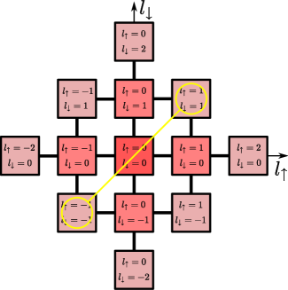
Figure 1: Particle number sectors ($(l_{\uparrow},l_{\downarrow})$) for a Hubbard system. Shells of sectors with the same Manhattan have the same color. The yellow line marks a possible combination of sectors to build a partition.

2.2 Hamilton operator of the sub-systems

It is expedient to introduce a combined site index $i\rightarrow(\alpha,i)$, where $\alpha\in\{A,B\}$ refers to the sub-systems and and henceforth $i\in\{1,\ldots,N_{h}\}$ enumerates the sites within each sub-system. The Hamiltonian can be decomposed into three parts

$$\hat{H} =\underbrace{\hat{H}_{A}+\hat{H}_{B}}_{:=\hat{H}_{0}}+\hat{H}_{AB}\;.$$

For spin-less fermions the parts of the Hamiltonian are

$$\hat{H}_{\alpha} = -t\sum_{\braket{i,j}}\hat{a}^{\dagger}_{\alpha,i}\hat{a}^{\phantom{dagger}}_{\alpha,j}+V\sum_{\braket{i,j}}\hat{n}_{\alpha,i}\hat{n}_{\alpha,j}\;;\quad\alpha\in\{A,B\}$$

$$\hat{H}_{AB} = \underbrace{-t{\sum_{i,j}}^{\prime}\bigg{(}\hat{a}^{\dagger}_{A,i}\hat{a}^{\phantom{dagger}}_{B,j}+\hat{a}^{\dagger}_{B,j}\hat{a}^{\phantom{dagger}}_{A,i}\bigg{)}}_{=:\hat{H}_{AB}^{\text{kin}}}+\underbrace{V{\sum_{i,j}}^{\prime}\hat{n}_{A,i}\hat{n}_{B,j}}_{=:\hat{H}_{AB}^{\text{int}}}$$

where $\sum^{\prime}$ indicates that the indices $i,j$ have to be chosen such that $(A,i)$ and $(B,j)$ belong to nearest neighbor sites.

For the Hubbard model the splitting yields

$$\hat{H}_{\alpha} =-t\sum_{\braket{i,j},\sigma}\hat{a}^{\dagger}_{\alpha,i,\sigma}\hat{a}^{\phantom{dagger}}_{\alpha,j,\sigma}+U\sum_{i}\hat{n}_{\alpha,i\uparrow}\hat{n}_{\alpha,i\downarrow}\;;\;\alpha\in\{A,B\}$$

$$\hat{H}_{AB} =-t{\sum_{i,j,\sigma}}^{\prime}\bigg{(}\hat{a}^{\dagger}_{A,i,\sigma}\hat{a}^{\phantom{dagger}}_{B,j,\sigma}+\hat{a}^{\dagger}_{B,j,\sigma}\hat{a}^{\phantom{dagger}}_{A,i,\sigma}\bigg{)}$$

In case of the spin-less fermion model there is a two-particle coupling term between the two sub-systems ($\hat{H}_{AB}^{\text{int}}$) which is detrimental for cluster perturbation theory (CPT or VCA, [6, 7]). In the present approach it does not make any difference at all.

Now, the particle numbers in the two sub-systems are not conserved, due to the inter-sub-system hopping, and in principle all particle numbers between $0$ and $N$ are conceivable for each sub-system. However, the most probable number of particles in the sub-systems is $N_{A}=N_{B}=N_{h}$. The particle number fluctuations in the two sub-systems is subject to the constraint $N_{A}+N_{B}=N$ and likewise for the two spin species $N_{A,\sigma}+N_{B,\sigma}=N_{h,\sigma}$. If the two sub-systems are decoupled, i.e. for $\hat{H}_{AB}=0$ the particle numbers in each sub-system are conserved as well.

In the case of the Hubbard model the partitioning concerns both spin species separately. A partition $(l_{\uparrow},l_{\downarrow})$ therefore represents the situation of $N_{A,\sigma}=N_{h\sigma}+l_{\sigma}$ and $N_{B,\sigma}=N_{h\sigma}-l_{\sigma}$, respectively. Typical configurations for partitions with $l=0$ and $l=\pm 1$ are depicted in fig. 2.

Figure 2: Partitioning the occupation number state space by number of particles in each sub-system. Here, representatives of each partition are depicted.

The eigenvectors of $\hat{H}_{0}$ are simply tensor products of the eigenvectors of the separate sub-system Hamiltonians $\hat{H}_{\alpha}$ and the eigenvalues are given by the sum of the corresponding eigenvalues. Let the eigenvalue problem of sub-system $\alpha$ with $N_{\alpha}=N+l$ electrons be given by

$$\hat{H}_{\alpha}\ket{\Psi_{\nu}^{(l)}}_{\alpha} =E^{(l)}_{\nu}\ket{\Psi_{\nu}^{(l)}}_{\alpha}\,.$$

Here the meaning of the the indices is as follows. The lower outer index $\alpha$ stands for the sub-system, the upper index ${(l)}$ represents the particle number ($N_{\alpha}=N_{h}+l$), and the lower index $\nu$ enumerates the eigenvalues and eigenvectors for this particle number. Note, that the eigenvalue spectrum is the same for both sub-systems if they are occupied by the same number of electrons.

The eigenvectors and eigenvalues of $H_{0}$ in partition $l$ are given by

$$\ket{\psi^{(l)}_{\nu}} :=\ket{\Psi_{\nu_{A}}^{(l)}}_{A}\otimes\ket{\Psi_{\nu_{B}}^{(-l)}}_{B}$$

$$E^{(l)}_{\nu} :=E^{(l)}_{\nu_{A}}+E^{(-l)}_{\nu_{B}}\;,$$

where the index $\nu$ represents the entire system with $\nu=(\nu_{A},\nu_{B})$.

Due to the missing coupling of the sub-systems, the eigenvalue problem of $\hat{H}_{0}$ has a strongly reduced complexity. If we add $\hat{H}_{AB}$ by perturbation theory, there will be a first order contribution only from the interaction term in the spin-less fermion case. The hopping terms do not contribute in first order, as they change the number of particles in the sub-systems.

The ground-state of $\hat{H}_{0}$ is obtained for $N_{A}=N_{B}=N_{h}$, i.e. it belongs to partition $l=0$. The second order energy correction is given by

$$\Delta E^{(2)} =\sum_{l=-N_{h}}^{N_{h}}{\sum_{\nu}}^{\prime}\frac{\big{|}\langle\psi^{(l)}_{\nu}|\hat{H}_{AB}|\psi^{(0)}_{0}\rangle\big{|}^{2}}{E^{(l=0)}_{0}-E^{(l)}_{\nu}}\;.$$

As usual $\sum^{\prime}$ indicates that $(l=0\wedge\nu=0)$ is excluded from the sum. Only $l=0$ and $l=\pm 1$ contribute to the energy correction, because only one electron can hop at a time across the border . In other words, the partitions $l=\pm 1$ come into play. The importance of the unperturbed eigenvectors of partitions $l=\pm 1$ is determined by the matrix the element $M_{\nu}^{(l=\pm 1)}:=\langle\psi^{(l=\pm 1)}_{\nu}|\hat{H}_{AB}|\psi^{(0)}_{0}\rangle$ and the inverse of the energetic distance $E^{(l=0)}_{0}-E^{(l)}_{\nu}$. The latter implies that low eigenstates of the unperturbed system are more important for the ground-state of the entire system than those with higher energies. In addition the kinetic coupling matrix element is driven by the hopping across the border and yields for the spin-less fermion model

$$M_{\nu}^{(l=\pm 1)} =-t{\sum_{ij}}^{\prime}\langle\psi^{(\pm 1)}_{\nu}|\big{(}\hat{a}^{\dagger}_{A,i}\hat{a}^{\phantom{\dagger}}_{B,j}+\hat{a}^{\dagger}_{B,j}\hat{a}^{\phantom{\dagger}}_{A,i}\big{)}|\psi^{(0)}_{0}\rangle$$

$$M_{\nu}^{(l=+1)} =-t{\sum_{ij}}^{\prime}\langle\psi^{(+1)}_{\nu_{A}}|\hat{a}^{\dagger}_{A,i}|\psi^{(0)}_{0}\rangle_{A}\langle\psi^{(-1)}_{\nu_{B}}|\hat{a}^{\phantom{\dagger}}_{B,j}|\psi^{(0)}_{0}\rangle_{B}\;.$$

Hence the relevance of eigenvectors of the sub-systems for the partition $l=+1$ depends on the occupation of the border sites in those states. We obtain a similar result for $M^{(l=-1)}_{\nu}$. From these considerations we can derive a criterion for the importance of the contribution of excited eigenvectors of the sub-systems to the total ground-state of the entire system.

We observe that the partitions $l=\pm 1$ contribute to second order energy or rather first order vector correction. The second order correction for the eigenvectors depend on the partitions $|l|=2$ and generally the $n$^th order correction requires $|l|=n$. This conclusion can also be obtained by starting a Lanczos iteration with the eigenvectors of the unperturbed system. Each Lanczos iteration then increase the required partition $|l|$ by one.

In the Hubbard model we have to deal with the pair $l=(l_{\uparrow},l_{\downarrow})$. Starting from $l=(0,0)$, to which the ground-state of $\hat{H}_{0}$ belongs, each Lanczos iteration modifies one of the values $l_{\sigma}$ by $\pm 1$. I.e. the first iteration includes all partitions with Manhattan distance 1 from the center $l=(0,0)$, the second iteration adds all partitions with Manhattan distance 2 and so forth.

3 Block structure of the Hamiltonian

The partitioning described in the previous section leads to a natural block structure of the Hamiltonian, which is depicted for the spin-less fermion model in fig. 3.

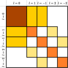
Figure 3: Block-structure of the Hamiltonian for the spin-less fermion model. As explained in the text, $N_{A}=N_{h}+l$ and $N_{B}=N_{h}-l$. Only partitions up to $l=\pm 2$ are depicted. White spaces represent blocks with zero matrix elements.

The upper-left block corresponds to partition $l=0$ that contains all many-body basis vectors in occupation number representation $\ket{\{n\}}$ with equal number of electrons in both sub-systems.

In general the basis vectors in partition $l$ are a tensor product of the contributions of the sub-systems

$$\ket{n^{(l)}_{\nu}} =\ket{n^{(l)}_{\nu_{A}}}_{A}\otimes\ket{n^{(-l)}_{\nu_{B}}}_{B}\;,$$

where $\nu=(\nu_{A},\nu_{B})$ enumerates the basis vectors of the entire system, while $\nu_{\alpha}$ enumerates the basis vectors of sub-system $\alpha$. The occupation number basis vectors of the two sub-systems have an outer index $\alpha\in\{A,B\}$ indicating the sub-system they belong to and they are constructed by the corresponding creation operators

$$\ket{n^{(l)}_{\nu}}_{\alpha} =\prod_{i=1}^{L_{h}}\big{(}a^{\dagger}_{\alpha,i}\big{)}^{n_{\nu}(\alpha,i)}\;\ket{0}_{\alpha}\;;$$

$$\sum_{i}n_{\nu}(\alpha,i) =N_{h}\pm l\;;\quad n_{\nu}(\alpha,i)\in\{0,1\}\;,$$

where $\ket{0}_{\alpha}$ represents the vacuum vector of sub-system $\alpha$. As a consequence of the representation by creation operators, the two factors of the tensor product do not commute. Commuting the factors yield an additional sign $(-1)^{N_{A}N_{B}}$. Similarly, there could be an additional sign when computing matrix elements in the tensor basis. Due to the tensor structure of the basis the computation of the matrix elements of $\hat{H}$ can be simplified significantly. The contribution of $\hat{H}_{0}$ to the diagonal block of partition $l$ reads

$$\big{(}H_{0}\big{)}^{(l,l)}_{\nu^{\prime},\nu} =\braket{n^{(l)}_{\nu^{\prime}_{A}}}{\hat{H}_{A}}{n^{(l)}_{\nu_{A}}}_{A}\delta_{\nu^{\prime}_{B},\nu_{B}}$$

$$+\delta_{\nu^{\prime}_{A},\nu_{A}}\braket{n^{(-l)}_{\nu^{\prime}_{B}}}{\hat{H}_{B}}{n^{(-l)}_{\nu_{B}}}_{B}\;.$$

As the diagonal blocks contain a fixed number of electrons in each sub-system there is no contribution stemming from the hopping part of $\hat{H}_{AB}$. However, in the spin-less fermion case the interaction term $\hat{H}_{AB}^{\text{int}}$ contributes to the diagonal block as well

$$\left(H^{\text{int}}_{AB}\right)^{(l,l)}_{\nu^{\prime},\nu} =V{\sum_{ij}}^{\prime}\braket{n^{(l)}_{\nu_{A}}}{\hat{n}_{A,i}}{n^{(l)}_{\nu_{A}}}_{A}\braket{n^{(-l)}_{\nu_{B}}}{\hat{n}_{B,j}}{n^{(-l)}_{\nu_{B}}}_{B}\;.$$

In both models under consideration the off-diagonal blocks are solely due to the hopping part in $\hat{H}_{AB}$, which changes the number of particles in the sub-systems by $\pm 1$. Consequently, only those blocks possess non-zero entries for which the partition indices differ by $|l^{\prime}-l|=1$ in the spin-less fermion case. In the case of the Hubbard model the condition for non-zero blocks reads $|l_{\uparrow}-l^{\prime}_{\uparrow}|+|l_{\downarrow}-l^{\prime}_{\downarrow}|=1$. I.e. in the $l_{\uparrow},l_{\downarrow}$ plain only those sites are coupled which have Manhattan distance 1. The corresponding spin resolved block structure is depicted in fig. 4.

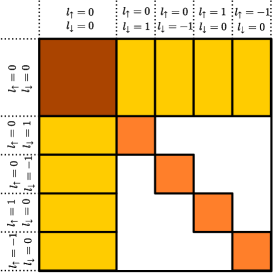
Figure 4: Block-structure of the Hubbard Hamiltonian. The meaning of $l_{\sigma}$ is explained in the text. Partitions up to Manhattan distance 1 are depicted. White spaces represent blocks with zero matrix elements.

For the Hubbard model the matrix elements in the off-diagonal blocks with $l^{\prime}>l$ are

$$\big{(}H_{AB}\big{)}^{(l^{\prime},l)}_{\nu^{\prime},\nu} =-t{\sum_{i,j,\sigma}}^{\prime}\langle n^{(l^{\prime})}_{\nu^{\prime}_{A}}|\hat{a}^{\dagger}_{A,i,\sigma}|n^{(l)}_{\nu_{A}}\rangle_{A}\langle n^{(-l^{\prime})}_{\nu^{\prime}_{B}}|\hat{a}^{\phantom{\dagger}}_{B,j,\sigma}|n^{(-l)}_{\nu_{B}}\rangle_{B}\;.$$

Due to the reordering of the creation/annihilation operators there is an additional sign factor $s=(-1)^{N_{h}+l}$. The matrix elements for $l^{\prime}<l$ follow from the hermiticity $M^{(l,l^{\prime})}_{\nu,\nu^{\prime}}=\big{(}M^{(l^{\prime},l)}_{\nu^{\prime},\nu}\big{)}^{\dagger}$. The matrix elements for the spin-less fermion case are obtained by restricting the sum over the spins to one spin species, to $\sigma=\uparrow$ say.

All block matrices have the structure

$$M^{(l^{\prime},l)}_{\nu^{\prime},\nu} =\sum_{\kappa}\big{(}M^{(A)}_{\kappa}\big{)}^{(l^{\prime},l)}_{\nu^{\prime}_{A},\nu_{A}}\big{(}M^{(B)}_{\kappa}\big{)}^{(l^{\prime},l)}_{\nu^{\prime}_{B},\nu_{B}}\;,$$ (1)

which will be exploited later on.

4 Ground-state eigenvalue problem

In the present approach we first solve the eigenvalue problem of the decoupled sub-systems for the different partitions.

$$\big{(}H_{0}\big{)}^{(l,l)}V^{(l)} =V^{(l)}D^{(l)}\;,$$

where $V^{(l)}$ is the unitary matrix of eigenvectors and the diagonal matrix $D^{(l)}$ contains the eigenvalues for partition $l$. As before, in the case of the Hubbard model $l$ stands for $l=(l_{\uparrow},l_{\downarrow})$.

We begin with $l=0$ $(l_{\uparrow}=l_{\downarrow}=0)$ and include gradually partitions of increasing Manhattan distance. We always include all partitions to a a given Manhattan distance, like $(l_{\uparrow},l_{\downarrow})\in\{(1,0),(-1,0),(0,1),(0,-1)\}$. From the set of eigenvectors $\{\ket{\psi^{(l)}_{\nu}}\}$ of these partitions we keep a certain number, which we call cropping number. Next we form the eigenvector of the entire system by a linear combination of those selected eigenvectors of the partitions included so far, i.e.

$$\ket{\Psi_{0}^{(l^{*})}} =\sum_{l=0}^{l^{*}}{\sum_{\nu}}C^{(l^{*})}_{l,\nu}\ket{\psi^{(l)}_{\nu}}\;.$$ (2)

If all partitions and all corresponding eigenvectors are included the result will be exact. Below, we will give a detailed study of the convergence as far as the upper partition number $l^{*}$ and the cropping numbers are concerned.

Given $l^{*}$ and the set of retained eigenvectors $\{\ket{\psi^{(l)}_{\nu}}\}$ for $l\leq l^{*}$, the coefficient vectors $C^{(l^{*})}_{l,\nu}$ is given by the eigenvectors of the matrix

$$\tilde{H}^{(l^{\prime},l)}_{\nu^{\prime},\nu} =\braket{\psi^{(l^{\prime})}_{\nu^{\prime}}}{\hat{H}}{\psi^{(l)}_{\nu}}\;,$$ (3)

spanned by the restricted set of unperturbed eigenvectors $\{\ket{\psi^{(l)}_{\nu}}\}$ for $l\leq l^{*}$. The approximated matrix $\tilde{H}$ has the same block structure in the partition numbers as the original matrix. Moreover, the matrix $\tilde{H}^{(l^{\prime},l)}$ of block $l^{\prime},l$ is given by

$$\tilde{H}^{(l^{\prime},l)} =\big{(}\tilde{V}^{(l^{\prime})}\big{)}^{\dagger}H^{(l^{\prime},l)}\tilde{V}^{(l)}\;,$$

where the matrix $\tilde{V}^{(l)}$ contains column-wise those the orthonormal eigenvectors of the diagonal block $H^{(0)}_{l,l}$, which are used in the expansion (2).

The contribution of $H_{0}$ to the diagonal block $\tilde{H}^{(l,l)}$ is diagonal, containing the retained eigenvalues $D^{(l)}$. For the computation of the block matrices resulting from $\hat{H}_{AB}$ one can exploit the tensor structure outlined in eq.(1) along with the tensor structure of $\tilde{V}^{(l)}$

$$\tilde{V}^{(l)}_{\nu^{\prime},\nu} =\tilde{V}^{(A,l)}_{\nu^{\prime}_{A},\nu_{A}}\tilde{V}^{(B,-l)}_{\nu^{\prime}_{B},\nu_{B}}\;,$$

where the columns of $\tilde{V}^{\alpha,l}$ contain the eigenvectors of $\hat{H}_{\alpha}$ retained by the cropping process. So we see that all operations are restricted to vectors and matrices of the size given by the sub-systems.

Fig. 5 illustrates the construction of the overall unitary matrix $\tilde{V}$.

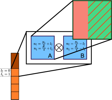
Figure 5: Illustration of the construction of the TSGSA basis $\tilde{V}$. Each partition corresponds to a fixed number of spin-up and spin-down particles in both sub-systems, which eigenvectors are combined tensorially (blue) to $\tilde{V}^{(l)}$. For each sub-system A and B the vectors are obtained by solving the corresponding eigenvalue problem. The eigenvectors are truncated e.g. by keeping only the vectors on the lower end of the spectrum (red).

The overall unitary transformation from the orthonormal occupation number basis to the orthonormal basis of the eigenvectors of $H_{0}$ has a block structure, corresponding to the partitions $(l_{\uparrow},l_{\downarrow})$. The partitions are enumerated with increasing Manhattan distance and within a shell of fixed distance $d$ counter clockwise beginning with $(l_{\uparrow}=d,l_{\downarrow}=0)$.

$$V =\begin{pmatrix}V^{(1)}&0&0&\ldots\\ 0&V^{(2)}&0&\ldots\\ 0&0&V^{(3)}&\ldots\\ \vdots&\vdots&&\ddots\end{pmatrix}\;,$$

where the columns are the eigenvectors of $H_{0}$ in the various partitions. Zeros are the corresponding zero matrices. If we only retain the restricted set of eigenvalues we obtain a $N_{b}\times m$ matrix, where $m$ is the number of retained eigenvectors

$$\tilde{V} =\begin{pmatrix}\tilde{V}^{(1)}&0&0&\ldots\\ 0&\tilde{V}^{(2)}&0&\ldots\\ 0&0&\tilde{V}^{(3)}&\ldots\\ \vdots&\vdots&&\ddots\end{pmatrix}\;,$$

the zero matrices are adjusted appropriately. $\tilde{V}$ is no longer unitary, but $\tilde{V}^{\dagger}\tilde{V}=I$ still holds for $I$ being the $m\times m$ identity matrix. The matrix $P:=\tilde{V}\tilde{V}^{\dagger}$ is the projection matrix into the space spanned by the retained eigenvectors. The above procedure corresponds to the eigenvalue problem of the projected Hamiltonian matrix $\tilde{H}=PHP$.

5 Numerical results

In order to determine how well the ground-state of a Hubbard model is approximated by the present approach a series of numerical simulations was performed and compared to exact values achieved by standard algorithms like the Lanczos method.

Croppings	$E$	$|E-E_{\text{exact}}|$	rel. error
80/60	-3.114643	0.1177	0.0361
80/60/30	-3.221613	0.0108	0.0033
80/60/40	-3.222737	0.0096	0.0030
80/60/50	-3.224861	0.0075	0.0023
80/60/50/20	-3.226303	0.0060	0.0019

Table 1: Ground-state energies of a Hubbard system ($L=12,N_{\uparrow}=N_{\downarrow}=6,pbc.,U=10$) as estimated by TSGSA compared to Exact Diagonalization (Lanczos). The exact solutions is $E_{0}=-3.232383$ and the basis size of the full Hamiltonian is 853,776. The first column shows the croppings for the individual partitions used (e.g. for the first line $80$ eigenmodes were used for the primary partition $l=0$; $60$ for the partition $l=\pm 1$, and so on).

As can be seen in tab. 1 the exact eigenvalues are approximated well by a comparably small vector space. Furthermore, the approximations can be enhanced by using a limited amount of additional eigenmodes of the sub-systems.

$L$	$N_{\sigma}$	Croppings	TSGSA	DMRG	rel. error
4	2	4/2	-0.882	-0.911	0.032
8	4	36/24	-1.937	-1.975	0.019
12	6	50/25	-2.949	-3.041	0.030
16	8	50/25	-3.961	-4.109	0.036
20	10	50/25	-5.021	-5.178	0.030
24	12	50/25	-6.090	-6.245	0.025

Table 2: TSGSA for multiple Hubbard system sizes (obc.), compared with DMRG.

A study for different system sizes can be seen in tab. 2. Here, the DMRG implementation by Reinhard Noak was used for comparison. Note, that the relative error is stable to decreasing with system size for constant number of eigenmodes taken into account. This is due to the fact that with increasing system sizes the primary partition becomes more important and hoppings over the sub-system boundary have less weight.

The largest Hubbard-type eigensystem calculation by exact diagonalization known to the author was preformed at the Earth Simulator [8]. The Hamiltonian used ($L=22$, $N_{\uparrow}=9$, $N_{\downarrow}=8$) had $1.59\cdot 10^{11}$ unknowns. Tab. 3 shows the convergence of a system ($L=22$, $N_{\uparrow}=N_{\downarrow}=11$) for the for physics important case of half-filling evaluated by the presented approach. The corresponding full basis size exceeds the mentioned world-record size by a factor of 3 ($5.0\cdot 10^{11}$). The calculations were performed using a parallelized implementation on a 8 QuadCore-Opteron CPU cluster at Graz University of Technology.

Croppings	$N_{\text{cores}}$	$t$ [s]	TSGSA	rel. error
25/25/25	5	2223	-5.5101	0.066
50/50/50	10	5123	-5.5305	0.061
75/75/75	10	15916	-5.5322	0.061
100/100/100	20	23369	-5.8169	0.013

Table 3: Convergence of the method for a Hubbard-type system ($L=22$, $N_{\uparrow}=N_{\downarrow}=11$, pbc., $U=10$), compared with DMRG (ground-state energy: $-5.8907$). $N_{\text{cores}}$ indicates the number of computation cores used, $t$ gives the total run-time in seconds.

6 Implementation

A key to the success of the algorithm is to find a scheme for calculation of more than just a few lowest eigenvectors, say in the order of 100. For this purpose an Implicitly Restarted Lanczos algorithm was used. Note, that the final, transformed Hamiltonian does not have to be calculated explicitly but a method for its application on a vector can be derived using the sub-system eigenvalues and eigenvectors.

Before combining the individual partitions to the effective Hamiltonian the calculations of the individual sub-systems can be done completely independent. So a parallelization of the calculation scheme could be done rather easily by dividing the different sub-system occupation configurations to different computation cores and solve the according eigensystems without need for communication. For larger systems this may not be practical, as the imbalance of numerical complexities among the different sub-systems makes a straight forward parallelization more inefficient. For this cases a parallelized version of the Implicitly Restarted Lanczos using algorithm was used.

The algorithm was implemented in the C++ programming language, as a parallelization framework OpenMPI was used.

7 Conclusions and Outlook

The presented approach may lead to a new way of performing calculations in strongly correlated material sciences. The results are promising compared to exact diagonalization. Although other sophisticated methods like DMRG, VCPT, or QMC exist, the TSGSA has the advantage of producing an explicit matrix representation. Furthermore it is not limited to one dimensional systems. It can be easily extended to more dimensions. In this case the off-equilibrium partitions may become more important due to larger interfaces between the sub-systems.

A further possibility for developing the algorithm are an intelligent way of selecting eigenmodes of the sub-system. It can be shown that many of them do not contribute to the full system ground-state.

References

• vonย der Linden [1992] W.ย vonย der Linden, A quantum monte carlo approach to many-body physics, Physics Reports 220 (1992) 53 โ€“ 162.
• Evertz [2003] H.ย G. Evertz, The loop algorithm, Advances in Physics 52 (2003) 1.
• Schollwรถck [2005] U.ย Schollwรถck, The density-matrix renormalization group, Rev. Mod. Phys. 77 (2005) 259โ€“315.
• Bekas and Saad [2005] C.ย Bekas, Y.ย Saad, Computation of smallest eigenvalues using spectral schur complements, SIAM J. Sci. Comput. 27 (2005) 458โ€“481.
• Bennighof and Lehoucq [2004] J.ย K. Bennighof, R.ย B. Lehoucq, An automated multilevel substructuring method for eigenspace computation in linear elastodynamics, SIAM Journal on Scientific Computing 25 (2004) 2084โ€“2106.
• Sรฉnรฉchal etย al. [2002] D.ย Sรฉnรฉchal, D.ย Perez, D.ย Plouffe, Cluster perturbation theory for hubbard models, Phys. Rev. B 66 (2002) 075129.
• Potthoff [2003] M.ย Potthoff, Self-energy-functional approach: Analytical results and the mott-hubbard transition, The European Physical Journal B - Condensed Matter and Complex Systems 36 (2003) 335โ€“348.
• Yamada etย al. [2008] S.ย Yamada, T.ย Imamura, M.ย Machida, 16.14 tflops eigenvalue solver on the earth simulator: Exact diagonalization for ultra largescale hamiltonian matrix, High-Performance Computing 4759 (2008) 402โ€“413.