Ab initio statistical mechanics of surface adsorption
and desorption: II. Nuclear quantum effects

Abstract

We show how the path-integral formulation of quantum statistical mechanics can be used to construct practical ab initio techniques for computing the chemical potential of molecules adsorbed on surfaces, with full inclusion of quantum nuclear effects. The techniques we describe are based on the computation of the potential of mean force on a chosen molecule, and generalise the techniques developed recently for classical nuclei. We present practical calculations based on density functional theory with a generalised-gradient exchange-correlation functional for the case of H₂O on the MgO (001) surface at low coverage. We note that the very high vibrational frequencies of the H₂O molecule would normally require very large numbers of time slices (beads) in path-integral calculations, but we show that this requirement can be dramatically reduced by employing the idea of thermodynamic integration with respect to the number of beads. The validity and correctness of our path-integral calculations on the H₂O/MgO (001) system are demonstrated by supporting calculations on a set of simple model systems for which quantum contributions to the free energy are known exactly from analytic arguments.

1 Introduction

In a recent paper [1], referred to here as paper I, we described an ab initio scheme for calculating the chemical potential and other thermodynamic properties of systems of adsorbed molecules, with full inclusion of entropy effects. We presented illustrative calculations based on density functional theory (DFT) for H₂O at low coverage on the MgO (001) surface, and showed how the chemical potential, and hence the desorption rate can be calculated without statistical-mechanical approximations, apart from the treatment of the nuclei as classical particles. That initial study was intended as a first step in developing ab initio methods for calculating the thermodynamic properties of adsorbate systems with better than chemical accuracy, i.e. better than 1 kcal/mol. As a contribution to these developments, we present here a practical scheme for including quantum nuclear effects in the ab initio statistical mechanics of adsorbates, and we report here some results for H₂O on MgO (001) at low coverage.

Quantum effects are likely to have a very significant effect on the properties of some adsorbates, particularly those containing protons, such as H₂O. The zero-point energies $\frac{1}{2}\hbar\omega$ of the symmetric and antisymmetric stretching modes and the bending mode of the H₂O molecules are 227, 233 and 99 meV respectively (5.23, 5.37 and 2.28 kcal/mol) [2]. Since partial or complete dissociation of adsorbed H₂O occurs quite commonly [3, 4, 5, 6, 7], it is clear that inclusion of quantum nuclear effects will sometimes be essential for accurate calculations. Needless to say, the future achievement of chemical accuracy will also depend crucially on the development of ab initio methods which go beyond conventional DFT, and that is currently the object of intensive research [8, 9, 10, 11]. However, the availability of improved ab initio methods is not our immediate concern here.

We emphasised in paper I that we aim to avoid statistical-mechanical approximations, and in particular we do not allow ourselves to resort to harmonic approximations, since these will not be satisfactory for the disordered adsorbates that are of ultimate interest. The overall strategy we shall present here closely resembles that of paper I, the main new feature being that the path-integral formulation of quantum mechanics is used to treat the nuclei. We noted in paper I that the chemical potential determines the ratio between the surface adsorbate density and the gas-phase density with which it is in equilibrium, and that this ratio can be expressed as an integral over the normalised density distribution $y(z)$ of molecules as a function of height $z$ above the surface. Since $y(z)$ can be expressed in terms of a potential of mean force $\phi(z)$, it can be computed from a sequence of thermal-equilibrium simulations in each of which the mean force on a chosen molecules is calculated, with the height $z$ of this molecule above the surface being constrained to have a fixed value. As we shall see, these relationships remain true in path-integral theory.

Path-integral statistical mechanics is based on the well known isomorphism between a quantum system of $N$ particles and a classical system of $N$ cyclic chains, each consisting of $P$ beads (time slices), with neighbouring beads in each chain being coupled by harmonic springs [12, 13, 14, 15, 16, 17, 18]. The meaning of this is that each cyclic chain represents the propagation of an individual quantum particle in imaginary time $\tau$ from $\tau=0$ to $\tau=\beta\hbar$. The ratio between the densities of adsorbed and gas-phase molecules, and the expression for this ratio in terms of a probability distribution $y(z)$ retain their validity when the nuclei are described by quantum mechanics, and we shall show that $y(z)$ can be expressed in terms of a potential of mean force $\phi(z)$ which can be derived from appropriately constrained simulations on the system of cyclic chains given by the path-integral isomorphism. In this sense, the generalisation of the methods of paper I to include quantum nuclear effects is in principle straightforward.

We shall use the example of H₂O on MgO (001) to show that it is practically feasible to calculate the chemical potential of an adsorbate using ab initio path-integral methods. The illustrative calculations are for the case of low coverage, i.e. isolated molecules, because we are not yet able to perform the statistical sampling at higher coverages. For isolated H₂O molecules on MgO (001), the changes of vibrational frequencies on adsorption are not large, so that quantum nuclear effects do not lead to great changes of the chemical potential. Nevertheless, the technical challenges of the calculations are interesting and substantial, because the high vibrational frequencies mean that the number of path-integral beads needs to be very high to achieve the required accuracy. To meet this challenge, we had to develop a new technique, in which thermodynamic integration is performed with respect to the number of beads. A significant part of the paper is concerned with the tests we have developed to demonstrate that our path-integral techniques work correctly.

The rest of the paper is organised as follows. The techniques themselves are laid out in Sec. 2: we start with a brief reminder of the methods developed in paper  I, and a summary of basic path-integral theory; then we explain how this theory can be used to create a path-integral generalisation of paper I that correctly yields the chemical potential with full inclusion of quantum nuclear effects; techniques for improving the computational efficiency and for performing thermodynamic integration with respect to the number of beads are also outlined; at the end of Sec. 2, we note the DFT techniques used in our practical calculations. Sec. 3 describes the tests we have performed on the path-integral machinery; these tests consist of simulations on a set of harmonic vibrational models involving the H₂O molecule acted on by various external fields, for which the results can be checked against values known from analytical formulas. The calculations on the chemical potential of the H₂O molecule adsorbed at finite temperature on MgO (001) are presented in Sec. 4. Finally, the implications of the work and the prospects for future applications and developments are discussed in Sec. 5.

2 Techniques

2.1 Chemical potential of adsorbed molecules: classical approximation

The classical theory of paper I is expressed in terms of the spatial distribution $\bar{\rho}(z)$ of molecules when there is full thermal equilibrium between the gas phase and the adsorbate. This distribution is defined so that $\bar{\rho}(z)\,d{\bf r}$ is the probability of finding a molecule in volume element $d{\bf r}$ at height $z$ above the surface, averaged over positions in the plane parallel to the surface. The detailed form of $\bar{\rho}(z)$ depends on which point within the molecule (e.g. centre of mass, position of a specified atom in the molecule, etc.) is chosen to construct the distribution; we refer to this as the “monitor point” [1]. In practice, it is convenient to work with the normalised function $y(z)\equiv\bar{\rho}(z)/\rho_{0}$, where $\rho_{0}$ is the mean density of molecules in the gas phase. The ratio of the density $\sigma$ of adsorbate molecules (number per unit area on the surface) and the gas-phase density $\rho_{0}$ is:

$$\sigma/\rho_{0}=\int_{-\infty}^{z_{0}}dz\,y(z)\;,$$ (1)

where $z_{0}$ is the height above the surface below which molecules are counted as being “adsorbed”. This ratio is also related to the excess chemical potentials of gas-phase and adsorbed molecules: $\sigma/\rho_{0}=d\exp[\beta\Delta\mu^{\dagger}(\sigma,T)]$, where $\Delta\mu^{\dagger}\equiv\mu_{\rm gas}^{\dagger}-\mu_{\rm ads}^{\dagger}$ is the difference of excess chemical potentials, defined in paper I, $\beta=1/k_{\rm B}T$ and $d$ is a length chosen for the purpose of defining $\mu_{\rm ads}^{\dagger}$. We refer to $\Delta\mu^{\dagger}$ as the “excess chemical potential difference” (ECPD). In principle, the choice of $z_{0}$ affects $\sigma$, and hence $\Delta\mu^{\dagger}$; but in most situations of interest $y(z)$ for $z<z_{0}$ is enormously greater than the gas-phase value $y(z\rightarrow\infty)=1$, so that in practice the dependence of $\sigma/\rho_{0}$ on $z_{0}$ can be neglected. For the same reason, the dependence of $\sigma/\rho_{0}$ and $\Delta\mu^{\dagger}$ on the choice of monitor point is extremely weak.

Since $y(z)>>1$ in the adsorption region $z<z_{0}$, the computation of $y(z)$ is a “rare event” problem. To overcome this problem, $y(z)$ is expressed as $y(z)=\exp(-\beta\phi(z))$, where the potential of mean force $\phi(z)$ represents the free energy of the entire system when the height of the molecule above the surface is constrained to have value $z$, with the condition $\phi(z\rightarrow\infty)=0$. To compute $\phi(z)$, we use the fact that $\langle F_{z}\rangle_{z}=-d\phi/dz$ is the $z$-component of the thermal average force acting on the molecule when its height is constrained to be $z$. In the practical calculations of paper I, ab initio molecular dynamics (m.d.) simulation was used to perform the constrained statistical sampling in the canonical ensemble, and hence the computation of $\langle F_{z}\rangle_{z}$. Integration of $\langle F_{z}\rangle_{z}$ then yields $\phi(z)$ and hence $y(z)$. Related techniques have been developed by other groups (see e.g. Ref. [19]).

2.2 Basic path-integral methods

We summarise briefly the path-integral background needed in this work; for details, the many reviews should be consulted [12, 13, 15, 16, 17, 18]. The Helmholtz free energy $F$ of a general system at temperature $T$ is $F=-k_{\rm B}T\ln Z$, where the partition function is $Z={\rm Tr}\,[\exp(-\beta\hat{H})]$, with $\beta=1/k_{\rm B}T$ and $\hat{H}=\hat{T}+\hat{V}$ the Hamiltonian of the system. Here $\hat{T}$ is the operator for the sum of kinetic energies of all the nuclei, and $\hat{V}=U(\{{\bf r}_{i}\})$ in the present work represents the electronic ground-state energy of the system when the nuclei are fixed at positions ${\bf r}_{i}$ ($i=1,2,\ldots N$).

As usual in path-integral theory, $Z$ is rewritten as $Z={\rm Tr}\,\left[(\hat{\rho}(\beta/P))^{P}\right]$, where $\hat{\rho}(\beta/P)=\exp(-(\beta/P)\hat{H})$ is the propagator for imaginary time $\beta\hbar/P$, which is approximated by the Trotter short-time formula:

$$\hat{\rho}(\beta/P)\simeq e^{-\beta\hat{V}/2P}\hat{\rho}_{0}(\beta/P)e^{-\beta\hat{V}/2P}\;,$$ (2)

with $\hat{\rho}_{0}(\beta/P)$ the free-particle propagator, given in coordinate representation by:

$$\rho_{0}({\bf R},{\bf R}^{\prime};\beta/P)\equiv\langle{\bf R}|\hat{\rho}_{0}(\beta/P)|{\bf R}^{\prime}\rangle=A_{P}\exp\left[-\sum_{i=1}^{N}\frac{m_{i}P}{2\beta\hbar^{2}}|{\bf r}_{i}-{\bf r}_{i}^{\prime}|^{2}\right]\;.$$ (3)

Here, ${\bf R}$ and ${\bf R}^{\prime}$ are points in the configuration space of the whole system, specified by the collections of positions $\{{\bf r}_{i}\}$ and $\{{\bf r}_{i}^{\prime}\}$, and the prefactor $A_{P}$ is given by:

$$A_{P}=\prod_{i=1}^{N}\left(\frac{m_{i}P}{2\pi\beta\hbar^{2}}\right)^{3/2}\;,$$ (4)

with $m_{i}$ the mass of nucleus $i$. The resulting approximation to the partition function, denoted here by $Z_{P}$, is then:

$$Z_{P}=\left(A_{P}\right)^{P}\int\prod_{s=0}^{P-1}\prod_{i=1}^{N}d{\bf r}_{is}\,\exp[-\beta(T_{P}(\{{\bf r}_{is}\})+V_{P}(\{{\bf r}_{is}\})]\;,$$ (5)

where ${\bf r}_{is}$ is the position of nucleus $i$ at time-slice $s$, and $T_{P}$ and $V_{P}$ are given by:

$$T_{P}(\{{\bf r}_{is}\}) = \sum_{s=0}^{P-1}\sum_{i=1}^{N}\frac{1}{2}\kappa_{P,i}|{\bf r}_{i\,s+1}-{\bf r}_{is}|^{2}$$

$$V_{P}(\{{\bf r}_{is}\}) = \frac{1}{P}\sum_{s=0}^{P-1}U(\{{\bf r}_{is}\})\;.$$ (6)

The spring constants $\kappa_{P,i}$ are given by $\kappa_{P,i}=m_{i}P/\beta^{2}\hbar^{2}$. The formula for $Z_{P}$ expresses the widely used approximation to the partition function of the $N$-particle quantum system in terms of the partition function of a classical system of $N$ cyclic chains, each consisting of $P$ “beads” (time slices), with neighbouring beads in each cyclic chain being coupled by harmonic springs. The exact partition function is recovered in the limit $P\rightarrow\infty$.

The spatial distributions of the positions of beads belonging to a particular time-slice in the classical system of cyclic chains have a special significance, because they are equal (in the $P\rightarrow\infty$ limit) to the corresponding equal-time spatial distributions in the quantum system. For example, the probability density of finding a particular nucleus at a particular spatial point ${\bf r}$ in the quantum system is equal to the probability density of finding a chosen bead on the cyclic chain representing that nucleus at point ${\bf r}$. This means that appropriate potentials of mean force in the classical cyclic-chain system allow us to calculate spatial probability distributions in the quantum system.

2.3 Constraints and mean force in path-integral scheme

In the case treated later of H₂O adsorbed on MgO (001), we could choose to take as monitor point the position of the O atom in the H₂O molecule. In that case, the normalised height distribution $y(z)$ of this monitor point in the quantum system is equal to the height distribution $y(z)$ of a chosen bead on the cyclic chain representing that O atom in the classical cyclic-chain system. Alternatively, if we took as monitor point the centre of mass of the H₂O molecule, i.e. the position ${\bf r}^{\rm cm}=(m_{\rm O}{\bf r}_{1}+m_{\rm H}{\bf r}_{2}+m_{\rm H}{\bf r}_{3})/(m_{\rm O}+2m_{\rm H})$ in an obvious notation, then the height distribution $y(z)$ of the $z$-component $z^{\rm cm}$ of this position in the quantum system is equal to the height distribution $y(z)$ of the quantity $z^{\rm cm}$ constructed from the O and H positions, all at the same chosen time-slice in the classical cyclic-chain system. Just as in the classical theory of paper I, the detailed form of $y(z)$ will depend on the choice of monitor point, but the integral $\int_{-\infty}^{z_{0}}dz\,y(z)$ will not depend appreciably on this choice (see above). In the quantum case, there are also other possible ways of constructing monitor points. One possibility is that we monitor the centre of mass of the centroids of the cyclic paths of the O and the two H atoms of the H₂O molecule. (The centroid of the cyclic chain of nucleus $i$ is the average ${\bar{\bf r}}_{i}=P^{-1}\sum_{s=1}^{P}{\bf r}_{is}$.) If we do this, then $y(z)$ for the classical system of cyclic chains does not necessarily correspond to any obervable of the quantum system. Nevertheless, the integral $\int_{-\infty}^{z_{0}}dz\,y(z)$ will still be the same as for other choices of monitor point. This choice of “centroid centre of mass” is the one that we use in the present work.

For any of the foregoing choices of monitor point, the distribution $y(z)$ can be computed from the potential of mean force $\phi(z)$, defined in the usual way as $y(z)=\exp(-\beta\phi(z))$, and the derivative $-d\phi/dz$ is $\langle F_{z}\rangle_{z}$, the mean value of the $z$-component of the force on the monitor point, when the $z$-component of the position of this monitor point is constrained to have a particular value.

2.4 Thermal sampling

When performing constrained thermal-equilibrium simulations of the cyclic chain system in order to calculate quantities such as $\langle F_{z}\rangle_{z}$, we can choose to use any simulation method that samples configuration space in the required manner. As in paper I, we use molecular dynamics (m.d.) simulation with Nosé [20] and Andersen [21] thermostats to perform sampling according to the canonical ensemble. We noted in paper I that with this approach we are free to choose the m.d. masses of the particles in any way that helps to improve the sampling efficiency, since spatial averages do not depend on these masses. When we use m.d. to perform thermal sampling of the system of cyclic chains, it is therefore essential to distinguish between the real nuclear masses $m_{i}$ appearing in the spring constants $\kappa_{i}$ from the m.d. “sampling masses” employed to sample the configuration space. In paper I, the sampling masses were chosen as $M_{\rm H}=8$, $M_{\rm O}=16$ and $M_{\rm Mg}=24$ a.u.

It is well known that if m.d. simulation is used to perform thermal sampling in the path-integral technique, with each bead on every chain being give a chosen mass, then the sampling efficiency is very poor, because of the very wide frequency spread of the vibration modes of each chain. The method we use to overcome this problem, which resembles the techniques used by other workers (see e.g. Ref. [22]), employs a mass matrix on each cyclic chain, so that the Hamiltonian governing the m.d. evolution is:

$$H=\frac{1}{2}\sum_{i=1}^{N}\sum_{s=0}^{P-1}\sum_{t=0}^{P-1}{\bf p}_{is}\cdot{\bf A}_{i\,st}\cdot{\bf p}_{it} + \frac{1}{2}\sum_{i=1}^{N}\sum_{s=0}^{P-1}\kappa_{i}|{\bf r}_{i\,s+1}-{\bf r}_{i\,s}|^{2}$$ (7)

$$+ P^{-1}\sum_{s=0}^{P-1}U({\bf r}_{1s}\,\ldots{\bf r}_{Ns})\;,$$

where ${\bf A}_{i\,st}$ are the elements of the (positive definite) inverse mass matrix for the cyclic chain representing nucleus $i$. Each mass matrix is chosen so that the vibration frequencies of all modes of each chain are similar, and so that the total mass of each chain has a value that would be suitable for the sampling mass in the classical system. This is achieved if we take:

$$A_{i\,st}=\frac{1}{M_{i}}\sum_{n=0}^{P-1}\frac{(C_{i}/P)\cos[2\pi n(s-t)/P]}{(C_{i}/P)+2\kappa_{i}(1-\cos(2\pi n/P))}\;.$$ (8)

The total sampling mass $M_{i}$ of each chain is chosen exactly as in the classical simulations of paper I (see above). The spring constants $C_{i}$ are chosen so that $(C_{i}/M_{i})^{1/2}$ is a typical frequency characterising the dynamics of nucleus $i$ in the classical simulations performed with masses $M_{i}$.

2.5 Switching number of beads

In some of our calculations, it is helpful to obtain the free energy by successive approximations. First, we calculate $F_{P}=-k_{\rm B}T\ln Z_{P}$ with a number of beads $P$ which is known to be insufficient. We then obtain a more accurate value $F_{2P}$ by adding the difference $F_{2P}-F_{P}$. If the accuracy is still insufficient, we repeat the process. There is a simple way of using thermodynamic integration to calculate the difference $F_{2P}-F_{P}$, which we now explain.

We define a generalised form of the free energy $F_{2P}$ for the system having $2P$ time slices by introducing weights $w_{s}$ ($s=0,\ldots 2P-1$) into the definition of the potential energy $V$ of eqn (6):

$$V_{2P}(\{{\bf r}_{is}\})=\frac{1}{2P}\sum_{s=0}^{2P-1}w_{s}U(\{{\bf r}_{is}\})\;.$$ (9)

The partition function $Z_{2P}$ and the free energy $F_{2P}$ are now functions of the $w_{s}$. We choose the $w_{s}$ to have the form $w_{s}=1+\lambda$ for even $s$ and $w_{s}=1-\lambda$ for odd $s$, so that the partition function $Z_{2P}$ is given by:

$$Z_{2P}=\left(A_{2P}\right)^{2P}\int\prod_{s=0}^{2P-1}\prod_{i=1}^{N}d{\bf r}_{is}\,\exp\left[-\beta\left(T_{2P}(\{{\bf r}_{is}\})+\frac{1}{2P}\sum_{s=0}^{2P-1}(1+(-1)^{s}\lambda)U(\{{\bf r}_{is}\})\right)\right]\;.$$ (10)

Clearly, $Z_{2P}$ and hence the free energy $F_{2P}$ depend on $\lambda$. From eqn (10), we readily obtain a formula for the variation of $F_{2P}$ with $\lambda$:

$$\partial F_{2P}/\partial\lambda=-\left\langle\frac{1}{2P}\sum_{s=0}^{P-1}\left(U(\{{\bf r}_{i\,2s+1}\})-U(\{{\bf r}_{i\,2s}\}\right)\right\rangle_{\lambda}\;.$$ (11)

Now the quantity $F_{2P}(\lambda=0)$ is just the usual approximation to the free energy calculated with $2P$ beads, as is clear from eqn (10). On the other hand, $F_{2P}(\lambda=1)$ is identical to $F_{P}(\lambda=0)$, which is the normal free energy calculated with $P$ beads. To see this, we note from eqn (10) that for $\lambda=1$ the potential term in the Boltzmann factor becomes:

$$\frac{1}{2P}\sum_{s=0}^{2P-1}(1+(-1)^{s})U(\{{\bf r}_{is}\})=\frac{1}{P}\sum_{s=0}^{P-1}U(\{{\bf r}_{i\,2s}\})\;,$$ (12)

which is the potential term that appears in $F_{P}(\lambda=0)$. But this means that we can integrate over all the positions ${\bf r}_{is}$ for odd $s$, since these no longer appear in the potential term. In doing the integrations, we use the fact that:

$$\left(A_{2P}\right)^{2}\int\prod_{i=1}^{N}d{\bf r}_{i\,2s+1}\!\!\!\!\! \!\!\!\!\!\exp\left[-\beta\sum_{i=1}^{N}\frac{1}{2}\kappa_{2P,i}|{\bf r}_{i\,2s+1}-{\bf r}_{i\,2s}|^{2}\right]\exp\left[-\beta\sum_{i=1}^{N}\frac{1}{2}\kappa_{2P,i}|{\bf r}_{i\,2s+2}-{\bf r}_{i\,2s+1}|^{2}\right]=$$ (13)

$$A_{P}\exp\left[-\beta\sum_{i=1}^{N}\frac{1}{2}\kappa_{P,i}|{\bf r}_{i\,2s+2}-{\bf r}_{i\,2s}|^{2}\right]\;,$$

which expresses the fact that $\hat{\rho}_{0}(\beta/(2P))\hat{\rho}_{0}(\beta/(2P))=\hat{\rho}_{0}(\beta/P)$. On using eqns (12) and (13) in eqn (10), we obtain $F_{2P}(\lambda=1)=F_{P}(\lambda=0)$.

It follows from this, and from eqn (11), that:

$$F_{2P}-F_{P}=\int_{0}^{1}d\lambda\,\left\langle\frac{1}{2P}\sum_{s=0}^{P-1}(U(\{{\bf r}_{i\,2s+1}\})-U(\{{\bf r}_{i\,2s}\})\right\rangle_{\lambda}\;.$$ (14)

This is the formula we use to calculate accurate values of free energy by successive approximation.

2.6 Ab initio techniques

Our practical simulations, like those of paper I, were made with the projector-augmented-wave implementation of DFT [23, 24], using the VASP code [25]. The DFT computations on all the $P$ path-integral images of the system (i.e. beads, or time-slices) are performed in parallel, with the operations for each image also distributed over groups of processors (typically, there are 16 processors allocated to each image for our full calculations on the MgO slab with or without H₂O). As in paper I, we use the PBE exchange-correlation functional [26], with a plane-wave cut-off of 400 eV and an augmentation-charge cut-off of 605 eV.

3 Testing the path-integral machinery

To verify that the path-integral techniques work correctly, we have used them to calculate the free energy changes when various external potentials are applied to an isolated H₂O molecule in free space. We have designed these potentials so that they mimic the changes that occur when a molecule passes from free space to the adsorbed state: the formation of vibrational and librational modes from free translations and rotations, and the alteration of intramolecular vibration modes. The potentials are designed so that the changes of free energy are known exactly. These tests also give us information about the number of beads $P$ needed to obtain results of specified accuracy. All the tests are performed with appropriately modified versions of the VASP code, with the technical settings mentioned above (Sec. 2.6).

3.1 Vibration of centre of mass

To mimic the conversion of free translations to vibrations, we introduce a potential that acts only the centre of mass of the molecule. This potential leaves molecular rotations and internal vibrations completely unchanged. We use the notation ${\bf r}_{i}$ for the positions of the three atoms in the molecule, with $i=1$, 2, 3 corresponding to the O atom and the two H atoms respectively. The position of the physical centre of mass is ${\bf r}^{\rm cm}\equiv(m_{\rm O}{\bf r}_{1}+m_{\rm H}({\bf r}_{2}+{\bf r}_{3}))/M$, where $M=m_{\rm O}+2m_{\rm H}$ is the total mass of the molecule. The total energy $U_{0}({\bf r}_{1},{\bf r}_{2},{\bf r}_{3})$ of the molecule in free space depends only on relative positions, such as ${\bf r}_{2}-{\bf r}_{1}$ and ${\bf r}_{3}-{\bf r}_{1}$, since it is translationally invariant. We add to $U_{0}$ an external potential $U_{\rm ext}(z^{\rm cm})$ depending only on the $z$-coordinate of the centre of mass. We want $U_{\rm ext}(z^{\rm cm})$ to consist of a harmonic well of spring constant $\alpha$ and depth $V_{0}$, and we want it to go to zero as $z\rightarrow\infty$. To obtain this, we adopt the form:

$$U_{\rm ext}(z) = -V_{0}+\frac{1}{2}\alpha(z-z_{0})^{2}\;,\;\;\;\;\;z<z_{1}$$ (15)

$$= -\frac{1}{2}\beta(z-z_{2})^{2}\;,\;\;\;\;\;z_{1}<z<z_{2}$$

$$= 0\;,\;\;\;\;\;z_{2}<z\;.$$

The constants are chosen so that $U_{\rm ext}$ and its first derivative are continuous at $z=z_{1}$. In this model, the rotational and internal-vibrational properties of the molecule are completely unchanged, and the only effect of $U_{\rm ext}$ is to produce harmonic oscillations of the centre of mass in the $z$-direction when $z<z_{1}$. We take the potential parameters and $T$ to be such that, when the molecule is in thermal equilibrium in the potential well, the probability of finding the centre of mass outside the region $z<z_{1}$ is negligible. Then the values of $\Delta\mu^{\dagger}$ in the quantum and classical cases are exactly $k_{\rm B}T\ln[2\sinh(\hbar\omega/2k_{\rm B}T)]$ and $k_{\rm B}T\ln(\hbar\omega/k_{\rm B}T)$, so that their difference (quantum minus classical) is $k_{\rm B}T\ln[\sinh(\hbar\omega/2k_{\rm B}T)/(\hbar\omega/2k_{\rm B}T)]$, where $\omega=\sqrt{\alpha/M}$ is the oscillation frequency of the centre of mass.

In the classical case, simulations are superfluous, since if the $z$-component of the centre of mass position is constrained to be $z$, then the force on the centre of mass is simply $F_{z}=-dU_{\rm ext}/dz$. In the quantum case, the coordinate we choose to constrain is the $z$-component of the centre of mass of the centroids ${\bar{z}}^{\rm cm}\equiv m_{\rm O}{\bar{z}}_{1}+m_{\rm H}({\bar{z}}_{2}+{\bar{z}}_{3}))/M$. Now it is readily shown that for a perfectly harmonic system in thermal equilibrium, the probability distribution of the path centroid is identical to that of the corresponding classical system. This implies that the mean force is also identical, and that the potentials of mean force in the quantum and classical cases can differ by at most a constant. In the present case of a piecewise harmonic $U_{\rm ext}$, the mean force is therefore the same in the quantum and classical systems, except for those ${\bar{z}}^{\rm cm}$ values for which beads are distributed on both sides of the “join” position $z_{1}$. Contributions to the quantum-classical difference of $\Delta\mu^{\dagger}$ therefore come only from this join region.

We have performed practical tests on this model for a variety of parameter values. An example is the case $\alpha=31.975$ eV/Ų, which gives a centre-of-mass oscillation frequency of 20.8 THz. With $|z_{1}-z_{0}|=0.5$ Å (we take $\beta=\alpha/25$), the centre of mass is almost completely confined to the region $z<z_{1}$ in both the quantum and classical cases at $T=100$ K. In this example, the exact quantum-classical difference of $\Delta\mu^{\dagger}$ is 23.2 meV. Our path-integral calculations of mean force for this case, performed with $P=8$ (spot checks with $P=16$ showed no appreciable differences), gave a difference of $23.2\pm 0.5$ meV, in perfect agreement with the exact value.

3.2 Libration of normal to molecular plane

To illustrate the conversion of free rotations to librations, we take a potential that acts on the vector normal to the molecular plane of the H₂O molecule. A suitable vector is:

$${\bf Q}_{\perp}=({\bf r}_{2}-{\bf r}_{1})\times({\bf r}_{3}-{\bf r}_{1})\;,$$ (16)

and we define the potential as:

$$V_{\rm ext}=\frac{1}{2}\alpha(n_{x}^{2}+n_{y}^{2})\;,$$ (17)

where the unit vector ${\bf n}$ is ${\bf Q}_{\perp}/|{\bf Q}_{\perp}|$. For $\alpha=0$, the molecule rotates freely, but for large positive $\alpha$ the normal executes small oscillations about the $z$-axis. If $\alpha$ is large enough, these oscillations are harmonic, and their frequencies are $\omega_{1}=(\alpha/I_{1})^{1/2}$ and $\omega_{2}=(\alpha/I_{2})^{1/2}$, where $I_{1}$ and $I_{2}$ are the moments of inertia for rotations about the two symmetry axes in the molecular plane. In-plane rotations (moment of inertia $I_{3}$) are unaffected. The free energy in the presence of $V_{\rm ext}$ is then the free energy of the two librations plus that of the free in-plane rotation. For the free energy in the absence of $V_{\rm ext}$, we use the standard expression for the free energy of an asymmetric top [27]. The free energy increase $\Delta F$ caused by switching on $V_{\rm ext}$ is thus known almost exactly. For our tests, we take $\alpha=2.00$ eV and $T=100$ K; under these conditions, the two librational modes are almost exactly in the quantum ground state. The free energy increase is $\Delta F=111$ meV.

We test the path-integral methods using a series of simulations with scaled external potential $\lambda V_{\rm ext}$, with $\lambda$ going from 0 to 1. The thermal average of $V_{\rm ext}$ in the path-integral system was calculated using $\lambda$ values of 0.0, 0.03, 0.06, 0.125, 0.25, 0.5 1.0, the reason for taking closely spaced $\lambda$ values near $\lambda=0$ being that the thermal average varies rapidly with $\lambda$ in this region (see Table 1). Numerical integration gives $\Delta F=102\pm 1$ meV, and $\Delta F=106\pm 1$ meV using $P=8$ and $P=16$ respectively. The small free energy difference obtained between $P=8$ and $P=16$ was also reproduced by directly calculating it using eqn (14), which gives $\Delta F_{16}-\Delta F_{8}=5\pm 1$ meV. Using eqn (14), we also obtained $\Delta F_{32}-\Delta F_{16}=1.5\pm 0.5$ meV, so that our best estimate for $\Delta F$ is $108.5\pm 2$ meV, which agrees with the exact value within the statistical errors.

	$P$
$\lambda$	8	16
0.0	$680\pm 11$	$664\pm 12$
0.03	$405\pm 12$	$443\pm 15$
0.06	$256\pm 8$	$247\pm 10$
0.125	$153\pm 4$	$144\pm 5$
0.25	$97\pm 2$	$101\pm 3$
0.5	$65\pm 1$	$70\pm 2$
1.0	$41\pm 1$	$47\pm 1$
$\Delta F$	$102\pm 1$	$106\pm 1$

Table 1: Thermal average $\langle V_{\rm ext}\rangle_{\lambda}$ as function of $\lambda$ and free energy change $\Delta F$. Units are meV.

3.3 Alteration of asymmetric stretch frequency

Surface adsorption will alter the intramolecular vibration frequencies, and to mimic this effect we apply an external potential having the form:

$$Z_{\rm ext}=\frac{1}{2}\kappa\xi^{2}\;,$$ (18)

where $\xi=({\bf r}_{2}+{\bf r}_{3}-2{\bf r}_{1})\cdot({\bf r}_{3}-{\bf r}_{2})$. Clearly, this has no effect on translations or rotations. By symmetry, $\xi$ remains zero in the presence of symmetric stretch and bond-angle oscillations. The only mode that is affected by $Z_{\rm ext}$ is thus the asymmetric stretch mode. In the absence of $Z_{\rm ext}$, our DFT calculations give the frequency $\omega_{\rm a}/2\pi=114.8$ THz. We have done tests with the value $\kappa=5.0236$ eV/Å⁴, which gives the increased frequency $\omega_{\rm a}/2\pi=151.2$ THz. At $T=100$ K, this vibrational mode is in its quantum ground state, so that the free energy change caused by $Z_{\rm ext}$ is $\Delta F=\frac{1}{2}\hbar(\omega_{\rm a}-\omega_{\rm a}^{0})=77.3$ meV.

In our path-integral simulations, we calculate the thermal average of $Z_{\rm ext}$ as a function of $\lambda$ in the presence of the scaled potential $\lambda Z_{\rm ext}$, with $\lambda$ going from 0 to 1. These calculations were done with several different numbers of time-slices $P$, going from 8 to 96. The computed results for the free energy change $\Delta F$ (Table 2) show that $P=96$ gives essentially exact results, and $P=64$ is also acceptable, but smaller values give seriously inaccurate results. This indicates that if we wished to calculate the chemical potential of adsorbed H₂O by brute force path-integral simulation, we would have to use at least $P=64$, which would be exceedingly expensive.

$P$	$\Delta F$(meV)
96	$78\pm 1.5$
64	$75\pm 1.5$
32	$59\pm 1.5$
16	$41\pm 1$
8	$21\pm 1.5$

Table 2: Free energy of the water molecule (in meV) in the external potential $Z_{\rm ext}$ at 100 K calculated using path integral simulations with different values of $P$.

This gives us an opportunity to test our technique of thermodynamic integration with respect to $P$. To apply this, we first calculate the free energy change as $\lambda$ goes from 0 to 1, using $P=8$. The resulting value of $\Delta F$ is in error by nearly 50 meV (Table 2). To correct this, we now calculate the free energy changes $F(P)-F(P/2)$, both for the free molecule and for the molecule acted on by $Z_{\rm ext}$. The resulting correction gives us $\Delta F(8)+\Delta F(8\rightarrow 64)=70\pm 6$ meV, which agrees within statistical error with the directly calculated value $\Delta F(64)=75\pm 1.5$ meV.

3.4 Other tests

As a further test of librational effects, we have compared path-integral calculations with quasi-exact results for the case where potentials act both on the normal to the molecular plane and on the direction of the molecular bisector. This is achieved by adding to the potential $V_{\rm ext}$ of Sec. 3.2 a potential $W_{\rm ext}$ defined by:

$$W_{\rm ext}=\frac{1}{2}\gamma q_{x}^{2}\;,$$ (19)

where $q_{x}$ is the $x$-component of the unit vector given by ${\bf q}=({\bf r}_{2}+{\bf r}_{3}-2{\bf r}_{1})/|{\bf r}_{2}+{\bf r}_{3}-2{\bf r}_{1}|$. The tests were done with $\gamma=2.00$ eV, which gives a frequency of $\sim 16$ THz for in-plane librations. The potential $W_{\rm ext}$ also induces a small change in the frequency of the asymmetric stretch mode. As before, the free energy change caused by switching on $V_{\rm ext}+W_{\rm ext}$ agrees within statistical error with the quasi-exact value.

In addition to all these tests on the ab initio free molecule, we have also made a completely different kind of test involving PMF calculations on the molecule as it is brought onto the surface of the rigid MgO slab (see Appendix). The methods are the same as those used for the full path-integral calculations presented in the next Section.

4 Full path-integral calculations for H₂O on MgO (001)

The PMF techniques of Sec. 2 are now applied to the full calculation of the ECPD $\Delta\mu^{\dagger}\equiv\mu_{\rm gas}^{\dagger}-\mu_{\rm ads}^{\dagger}$, both with and without nuclear quantum effects. We denote the difference of $\Delta\mu^{\dagger}$ values (quantum minus classical) by $(\Delta\mu^{\dagger})_{\rm qc}$. We know from the tests of Sec. 3 that in order to obtain values for $(\Delta\mu^{\dagger})_{\rm qc}$ that are correct to better than $\sim 5$ meV, the number of beads $P$ must be no less than 64. Our strategy is to perform all PMF calculations with $P=8$, and then to correct the results by performing thermodynamic integration with respect to the number of beads, for the free molecule, for the slab-molecule system, and for the clean slab. All the parameters of the simulated system were set exactly as in paper I: we use a 3-layer $2\times 2$ slab (16 ions per layer, for a total of 48 ions per repeating unit of the MgO slab), with a vacuum gap of 12.7 Å, a lattice parameter of 4.23 Å (the PBE bulk equilibrium value at $T=0$ K), and $\Gamma$-point electronic sampling. We use a time-step of 1 fs, and m.d. sampling masses of 24.3, 16.0 and 8.0 a.u. for Mg, O and H, in conjunction with the mass-matrix technique (Sec. 2.4). With these parameters, the conservation of the constant of motion was of the same quality as that obtained in the classical simulation of paper I. The calculations were performed at $T=100$ K, with an Andersen thermostat [21], and constrained simulations were made at 13 different values of height $z$. We find that simulations of 20 ps suffice to give a statistical error on the PMF at its minimum of less than 6 meV, which, as shown in paper I (Appendix A), is approximately equal to the error in the ECPD $\Delta\mu^{\dagger}$.

The mean forces $\langle F_{z}\rangle_{z}$ and the PMFs $\phi(z)$ calculated with $P=8$ and $P=1$ (classical case) are shown in Fig. 1. We see that quantum effects are small, but are easily detectable within the statistical errors. In particular, we notice that the classical mean force is slightly lower than the quantum value almost everywhere, apart from the region $4.8\leq z\leq 5.2$ Å, where it is higher. By integrating the PMFs, we obtain a quantum-classical difference of EPCD of $(\Delta\mu^{\dagger})_{\rm qc}=-22\pm 7$ meV.

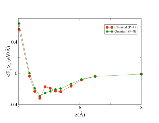
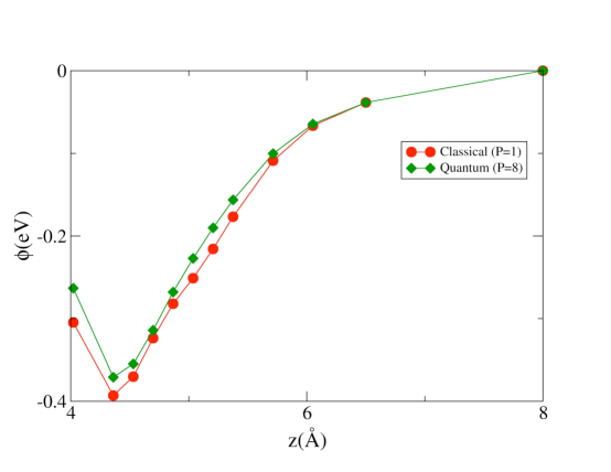
Figure 1: Mean force $\langle F_{z}\rangle_{z}$ and potential of mean force $\phi(z)$ of H₂O on MgO (001) calculated here using path-integral simulation with $P=8$ beads (diamonds), compared with the classical results of paper I (circles). Units are Å and eV. Statistical error bars are smaller than the size of the points.

In computing the free energy changes on going from $P=8$ to $P=64$ for the isolated molecule and slab-molecule system, we used 4, 3 and 2 values of $\lambda$ for the $8\rightarrow 16$, $16\rightarrow 32$ and $32\rightarrow 64$ contributions (simulations at $\lambda=0$ are unnecessary, since $\langle U_{P}-U_{2P}\rangle_{\lambda=0}=0$). For the clean slab, we needed only two values of $\lambda$, since the $P=8\rightarrow 64$ corrections for this system are rather small. In Fig. 2, we show the values of $\langle U_{P}-U_{2P}\rangle_{\lambda}$ as a function of $\lambda$ for the three systems. We see that most of the nuclear quantum contribution comes from the step $8\rightarrow 16$, but the other two contributions are not negligible. However, when we combine the contributions from the three systems, the three contributions $8\rightarrow 16$, $16\rightarrow 32$ and $32\rightarrow 64$ are all very small, and the total change of $\Delta\mu^{\dagger}$ (64 beads minus 8 beads) amounts to only $-8\pm 3$ meV.

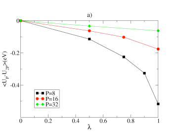
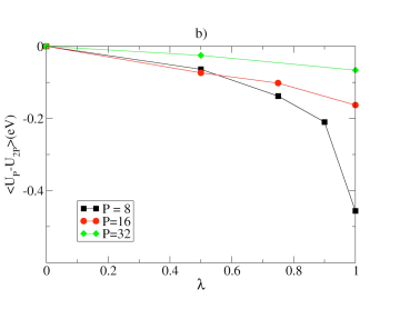
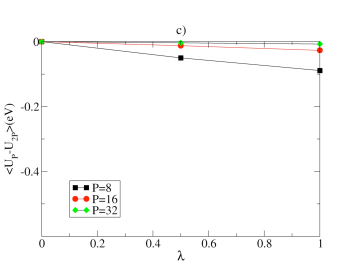
Figure 2: Computed results for the quantity $\langle U_{P}-U_{2P}\rangle_{\lambda}$ (eV units) used to calculate the difference $F_{P}-F_{2P}$ between path-integral free energies for numbers of beads $P$ and $2P$. Panels (a), (b) and (c) show results for the slab-molecule system, the free molecule, and the bare slab respectively. Results for $P=8$, 16 and 32 are shown by squares, circles and diamonds. Statistical error bars are smaller than the size of the points.

Including now the correction due to going from $P=8$ to 64 beads, the final result for the nuclear quantum correction to the ECPD comes to $(\Delta\mu^{\dagger})_{\rm qc}=-30\pm 8$ meV.

5 Discussion and conclusions

The main purpose of this work has been to establish the practical possibility of calculating the chemical potential of adsorbed molecules using ab initio methods with full inclusion of nuclear quantum effects, but without resorting to harmonic approximations. We have shown that within the path-integral formulation of quantum mechanics this can be achieved by a generalisation of the ab initio methods that have already been used for the case of classical nuclei. In particular, the method based on computing the mean force acting on a single molecule in a series of constrained simulations generalises naturally to the path-integral framework. Our practical calculations on the chemical potential of H₂O on MgO (001) at low coverage show that available computer power suffices to reduce statistical errors to $\sim 10$ meV, if required. However, this is achievable only thanks to a techniques we have introduced for performing thermodynamic integration with respect to the number of beads (time-slices).

Naturally, future calculations of this kind will be of greatest interest when the nuclear quantum effects are large, and this will typically be true when very high intra-molecular vibrational frequencies are strongly affected by surface adsorption. Many examples of this are known, among which are water adsorption on both oxide and metal surfaces. For example, it has recently been shown that for water layers on some transition-metal surfaces the traditional distinction between covalent and hydrogen bonds can be partially or almost entirely lost [35]. However, for the H₂O/MgO (001) case studied here, nuclear quantum effects turn out to have a rather small net effect on the chemical potential, changing it by only 30 meV. This is not because the the zero-point energies are small (they are not), but because the intra-molecular vibrational frequencies of H₂O are not greatly changed on adsorption, and the effects of the changes are partly cancelled by the zero-point energies of the new molecule-surface modes created from translational and rotational modes of the free molecule. However, this will not be the case for many other water-adsorption systems, and we believe there is ample scope for interesting applications of our methods.

The practical calculations of this paper and paper I were on the H₂O/MgO (001) system at very low coverage, where interactions between adsorbed molecules can be ignored. However, we focused on this low-density limit out of necessity rather than choice. In most practical situations, intermolecular interactions play a major role, and certainly have a strong effect on thermal desorption rates and on the surface coverage in thermal equilibrium with a given gas-phase pressure. For ab initio statistical mechanics, calculations away from the low-density limit present two kinds of problem. First, the simulated systems need to be larger, in order to reduce system-size errors to an acceptable level. Second, memory times, and hence sampling times usually become much longer, because molecules tend to hinder each other’s translational and rotational motion. We know from our own work with empirical interaction models for H₂O/MgO (001) [33, 34] that, if we use the PMF approach, simulation times need to be at least 10 times as long at higher coverage than in the low-density limit. Nevertheless, with empirical interaction models, the calculation of adsorption isotherms (coverage as a function of chemical potential at fixed $T$) has been routinely practiced for many years, using grand canonical Monte Carlo (GCMC) [36, 37] and other techniques. It is clearly an important challenge for the immediate future to develop the techniques that will allow the same to be done with ab initio methods, and ultimately with ab initio path-integral methods. This will not necessarily be done with GCMC, though, because there may be more effective strategies.

Before concluding, we return briefly to the issue of improving ab initio accuracy, which we noted in the Introduction. Improvements are much needed, because DFT energetics of surface systems often depends significantly on the approximation used for exchange-correlation energy. Increasingly effective methods for applying highly-correlated quantum chemistry to extended systems [32, 28, 8, 29, 30, 31], the growing power of quantum Monte Carlo techniques [38, 39, 40, 41, 42, 9, 43], and progress with improved van der Waals DFT functionals [44] give promising signs that ab initio calculations on surface adsorbates with chemical accuracy or better are now coming within reach. These improvements will enhance the importance of being able to account for nuclear quantum corrections.

In conclusion, we have presented ab initio path-integral techniques which allow the calculation of the chemical potential of adsorbate molecules in thermal equilibrium, with the nuclei treated fully quantum mechanically. We have verified that the techniques give correct results by applying them to a set of models where the quantum corrections are exactly known. We have demonstrated the practical effectiveness of the techniques by applying them to the H₂O molecule adsorbed on the MgO (001) surface. We find that in this case nuclear quantum corrections to the chemical potential are only $\sim 30$ meV, but we have noted the possibility of applying the techniques to other systems where the corrections should be much larger.

Appendix: Test by adsorption on the rigid surface

In Sec. 3, we presented some tests of the path-integral techniques applied to models in which carefully chosen external potentials act on the molecule in free space. We summarise here a different kind of test, in which full path-integral calculations of the mean force as a function of height $z$ are used to calculate the chemical potential for surface adsorption, but with the MgO slab held rigid. These calculations are of exactly the same kind as the full calculations reported in Sec. 4, in that the entire system (MgO slab + H₂O molecule) is treated by DFT. However, we modify the system to ensure that it is closely harmonic with the molecule on the surface by adding artificial potentials of the kind already used in Sec. 3; this enables us to obtain quasi-exact values for the difference between the quantum and classical values of the chemical potential, which can be used to validate the path-integral methods.

The potentials that we have added to the DFT total energy to ensure almost harmonic behaviour have the form $V_{\rm ext}+W_{\rm ext}+K_{\rm ext}$. Here, $V_{\rm ext}$ is the potential acting on the normal to the molecular plane (Sec. 3.2), and $W_{\rm ext}$ is the potential acting on the molecular bisector (Sec. 3.4). The potential $K_{\rm ext}$ is a harmonic potential confining the motion of the molecular centre of mass in the plane parallel to the surface:

$$K_{\rm ext}=\frac{1}{2}\beta((x^{\rm cm})^{2}+(y^{\rm cm})^{2})\;,$$ (20)

with ${\bf r}^{\rm cm}$ the centre-of-mass position defined in Sec. 3.1. The $V_{\rm ext}$ potential is zero when the normal to the molecular plane points along the $z$-axis, which in the present context means the normal to the MgO (001) surface. The $W_{\rm ext}$ potential is zero when the molecular bisector points along the $x$-axis, and we take this to be a cubic axis of the crystal parallel to the surface. Finally, we take the $K_{\rm ext}$ potential to be zero at a point near a surface Mg ion. All three potentials $V_{\rm ext}$, $W_{\rm ext}$ and $K_{\rm ext}$ are invariant under translation of the molecule along the $z$-direction, and they act on the molecule in exactly the same way when it is far from the surface as when it is on the surface. The values of the spring constants $\alpha$, $\gamma$ and $\beta$ are chosen to be 2.00 eV, 2.00 eV and 10.0 eV/Ų respectively. From the harmonic vibration frequencies of the molecule on the surface and in free space, we easily derive the chemical potential $\Delta\mu^{\dagger}$ at any temperature $T$, using either classical or quantum theory. At $T=100$ K, we find that the difference $(\Delta\mu^{\dagger})_{\rm qc}$ (quantum minus classical) has the small value 9 meV.

As in Sec. 4, the potential of mean force calculations were performed with 8 beads, and the results were then corrected by thermodynamic integration with respect to number of beads, going from 8 to 16 to 32 to 64 beads. For comparison, the PMF calculations were also performed with classical nuclei. We find that with 8 beads the quantum-classical difference $(\Delta\mu^{\dagger})_{\rm qc}$ is $-13\pm 1$ meV, which differs substantially from the quasi-exact value of 9 meV. However the corrections from thermodynamic integration over the number of beads are large, and they do not cancel between gas and surface. In the gas phase, the change of free energy on going from 8 to 64 heads is $198\pm 3$ meV, while on the surface the change is $180\pm 4$ meV. This means that going from 8 to 64 beads stabilises the molecule on the surface by 18 meV, and the resulting corrected value for $(\Delta\mu^{\dagger})_{\rm qc}$ comes to $5\pm 5$ meV, which agrees well with the quasi-exact value within statistical errors.

References

- [1] D. Alfè and M. J. Gillan, J. Chem. Phys., 127, 114709 (2007).
- [2] J. Tennyson, N. F. Zobov, R. Williamson, O. L. Polyansky, P. F. Bernath, J. Phys. Chem. Ref. Data, 30, 735 (2001).
- [3] W. Langel and M. Parrinello, Phys. Rev. Lett., 73, 504 (1994).
- [4] L. Giordano, J. Goniakowski and S. Suzanne, Phys. Rev. Lett., 81, 1271 (1998).
- [5] P. J. D. Lindan, N. M. Harrison and M. J. Gillan, Phys. Rev. Lett., 80, 762 (1998).
- [6] R. Schaub, P. Thostrup, N. Lopez, E. Laegsgaard, I. Stensgaard, J. K. Norskov and F. Besenbacher, Phys. Rev. Lett., 87, 266104 (2001).
- [7] Y. Yu, Q. Guo, S. Liu, E. Wang, P. Moller, Phys. Rev. B, 68, 115414 (2003).
- [8] B. Li, A. Michaelides and M. Scheffler, Surf. Sci., 602, L135 (2008).
- [9] J. Ma, D. Alfè, A. Michaelides and E. G. Wang, J. Chem. Phys., 130, 154303 (2009).
- [10] C. Muller, K. Hermansson and B. Paulus, Chem. Phys., 362, 91 (2009).
- [11] B. Paulus and K. Rosciszewski, Int. J. Quantum Chem., 109, 3055 (2009).
- [12] R. P. Feynman and A. R. Hibbs, Quantum Mechanics and Path Integrals (McGraw-Hill, New York, 1965).
- [13] R. P. Feynman, Statistical Mechanics (Addison-Wesley, Redwood City, 1972).
- [14] M. Parrinello and A. Rahman, J. Chem. Phys., 80, 860 (1984).
- [15] B. J. Berne and D. Thirumalai, Annu. Rev. Phys. Chem., 37, 401 (1986).
- [16] M. J. Gillan, in Computer Modelling of Fluids, Polymers and Solids, ed. C. R. Catlow, S. C. Parker and M. P. Allen (Kluwer, Dordrecht, 1990).
- [17] D. Marx and M. Parrinello, J. Chem. Phys., 104, 4077 (1996).
- [18] M. E. Tuckerman, D. Marx, M. L. Klein and M. Parrinello, J. Chem. Phys., 104, 5579 (1996).
- [19] K. A. Fichthorn and R. A. Miron, Phys. Rev. Lett., 89, 196103 (2002).
- [20] S. Nosé, Molec. Phys, 52, 255 (1984); J. Chem. Phys., 81, 511 (1984).
- [21] H. C. Andersen, J. Chem. Phys., 72, 2384 (1980).
- [22] S. D. Ivanov, A. P. Lyubartsev and A. Laaksonen, Phys. Rev. E, 67, 066710 (2003).
- [23] P. Blöchl, Phys. Rev. B, 50, 17953 (1994).
- [24] G. Kresse and D. Joubert, Phys. Rev. B, 59, 1758 (1999).
- [25] G. Kresse and J. Furthmüller, Phys. Rev. B, 54, 11169 (1996).
- [26] J. P. Perdew, K. Burke and M. Ernzerhof, Phys. Rev. Lett., 77, 3865 (1996).
- [27] K. F. Stripp and J. G. Kirkwood, J. Chem. Phys., 19, 1131 (1951).
- [28] F. R. Manby, D. Alfè, M. J. Gillan, Phys. Chem. Chem. Phys., 8, 5178 (2006).
- [29] S. Nolan, M. J. Gillan, D. Alfè, N. R. Allan, and F. R. Manby, Phys. Rev. B, 80, 165109 (2009).
- [30] M. Marsman, A. Gruneis, J. Paier, G. Kresse, J. Chem. Phys., 130, 184103 (2009).
- [31] J. Harl and G. Kresse, Phys. Rev. Lett., 103, 056401 (2009).
- [32] B. Paulus, Phys. Rep., 248, 1 (2006).
- [33] H. Fox, M. J. Gillan and A. P. Horsfield, Surf. Sci., 601, 5016 (2007).
- [34] H. Fox, M. J. Gillan and A. P. Horsfield, Surf. Sci., 603, 2171 (2009).
- [35] X. Z. Li, M. I. J. Probert, A. Alavi and A. Michaelides, Phys. Rev. Lett., 104, 066102 (2010).
- [36] G. E. Norman and V. S. Filinov, High Temp. (USSR), 7, 216 (1969).
- [37] D. Frenkel and B. Smit, Understanding Molecular Simulation, 2nd edition (Academic Press, San Diego, 2002), chapter 5.
- [38] D. Alfè and M. J. Gillan, J. Phys. Cond. Matt., 18, L435 (2006).
- [39] I.G. Gurtubay and R.J. Needs, J. Chem. Phys., 127, 124306 (2007).
- [40] N.D. Drummond and R.J. Needs, Phys. Rev. Lett., 99, 166401 (2007).
- [41] M. Pozzo and D. Alfè, Phys. Rev. B, 78, 245313 (2008); Phys. Rev. B, 77, 104103 (2008).
- [42] S. J. Binnie, E. Sola, D. Alfè, and M. J. Gillan, Mol. Sim., 35 609 (2009).
- [43] E. Sola and D. Alfè, Phys. Rev. Lett., 103, 078501 (2009).
- [44] J. Klimeš, D. R. Bowler and A. Michaelides, J. Phys: Condens. Matter, 22, 022201 (2010).