Quantum Phase Transitions in Bosonic Heteronuclear Pairing Hamiltonians

Abstract

We explore the phase diagram of two-component bosons with Feshbach resonant pairing interactions in an optical lattice. It has been shown in previous work to exhibit a rich variety of phases and phase transitions, including a paradigmatic Ising quantum phase transition within the second Mott lobe. We discuss the evolution of the phase diagram with system parameters and relate this to the predictions of Landau theory. We extend our exact diagonalization studies of the one-dimensional bosonic Hamiltonian and confirm additional Ising critical exponents for the longitudinal and transverse magnetic susceptibilities within the second Mott lobe. The numerical results for the ground state energy and transverse magnetization are in good agreement with exact solutions of the Ising model in the thermodynamic limit. We also provide details of the low-energy spectrum, as well as density fluctuations and superfluid fractions in the grand canonical ensemble.

I Introduction

In the last few years there has been considerable experimental and theoretical interest in studying Feshbach resonances between different atomic species and isotopes. This activity encompasses pairing interactions and molecule formation in a wide variety of Fermi–Fermi, Bose–Fermi, and Bose–Bose mixtures. Such systems provide many possibilities for novel phases and phenomena, ranging from dipolar condensates Santos:Dipolar ; Baranov:Dipolar to highly controllable chemical reactions Ospelkaus:Reactions . Recent examples include heteronuclear resonances in ${}^{85}{\rm Rb}$–${}^{87}{\rm Rb}$ Papp:Hetero ; Papp:Tunable ; Ticknor:Multiplet , ${}^{41}{\rm K}$–${}^{87}{\rm Rb}$ Weber:Assoc ; Thalhammer:Double ; Thalhammer:Coll ; Barontini:Obs ; Catani:Entropy ; Lamporesi:Mixed , ${}^{39}{\rm K}$–${}^{87}{\rm Rb}$ Simoni:Near , and ${}^{87}{\rm Rb}$–${}^{133}{\rm Cs}$ Pilch:Obs Bose mixtures over a range of experimental parameters.

Motivated by these developments, we recently investigated the phase diagram of two-component bosons pairing in an optical lattice Bhaseen:Feshising . Amongst our findings, we identified a paradigmatic Ising quantum phase transition occurring within the second Mott lobe. The principal aim of this manuscript is to provide a more detailed overview of this heteronuclear system, and to extend the scope of physical observables presented in Ref. Bhaseen:Feshising . We expand our previous exact diagonalization results in several directions, and confirm the additional Ising critical exponents, $\alpha=0$, $\gamma=7/4$ and $\delta=15$. We also provide results for the low-energy spectrum, as well as density fluctuations and superfluid fractions in the grand-canonical ensemble. We supplement this with a discussion of the evolution of the phase diagram with system parameters, and its direct connection to Landau theory.

The layout of this manuscript is as follows. In Sec. II we describe the heteronuclear model with Feshbach interactions. In Secs. III and 8 we discuss the mean field phase diagram and the Landau theory description. In Sec. V we focus on the Mott states and present a derivation of the effective quantum Ising model. We confirm these findings in Sec. VI by exact diagonalization of the one-dimensional bosonic Hamiltonian. We conclude in Sec. VII. We incorporate the principal results of Ref. Bhaseen:Feshising .

II The Model

We consider two-component bosons with a “spin” index $\downarrow,\uparrow$, which may be different hyperfine states, isotopes or species. These components may form molecules, $m$, as described by the Hamiltonian

$$H =\sum_{i\alpha}\epsilon_{\alpha}n_{i\alpha}-\sum_{\langle ij\rangle}\sum_{\alpha}t_{\alpha}\left(a_{i\alpha}^{\dagger}a_{j\alpha}+{\rm h.c.}\right)$$ (1)

$$\hskip 28.45274pt+\sum_{i\alpha\alpha^{\prime}}\frac{U_{\alpha\alpha^{\prime}}}{2}:n_{i\alpha}n_{i\alpha^{\prime}}:+\,H_{\text{F}}.$$

Here, $a_{i\alpha}$ are Bose annihilation operators, where $i$ labels the lattice sites, $n_{i\alpha}=a_{i\alpha}^{\dagger}a_{i\alpha}$, and $\alpha=\downarrow,\uparrow,m$; $\epsilon_{\alpha}$ are on-site potentials, $t_{\alpha}$ are hopping parameters, $\langle ij\rangle$ denotes summation over nearest neighbor bonds, and $U_{\alpha\alpha^{\prime}}$ are interactions. Molecule formation is described by the s-wave interspecies Feshbach resonance term

$$H_{\text{F}}=g\sum_{i}(a^{\dagger}_{im}a_{i\uparrow}a_{i\downarrow}+{\rm h.c.}).$$ (2)

Similar problems have been studied in the continuum limit with s-wave Zhou:PS and p-wave resonances Radzi:spinor . Closely related homonuclear systems have also been considered in the continuum Timmermans:Feshbach ; Rad:Atmol ; Romans:QPT ; Koetsier:Bosecross ; Radzi:Resonant and on the lattice Dickerscheid:Feshbach ; Sengupta:Feshbach ; Rousseau:Fesh ; Rousseau:Mixtures . Normal ordering implies ${:n_{i\alpha}n_{i\alpha}:}=n_{i\alpha}(n_{i\alpha}-1)$ for like species, and ${:n_{i\alpha}n_{i\alpha^{\prime}}:}=n_{i\alpha}n_{i\alpha^{\prime}}$ for distinct species. For simplicity we consider hardcore atoms and molecules and set $U_{m\uparrow}=U_{m\downarrow}\equiv U$ and $U_{\uparrow\downarrow}\equiv V$. We begin work in the grand canonical ensemble with $H_{\mu}=H-\mu_{\rm T}N_{\rm T}-\mu_{\rm D}N_{\rm D}$, where $N_{\rm T}\equiv\sum_{i}(n_{i{\uparrow}}+n_{i\downarrow}+2n_{im})$ is the total atom number, including a factor of two for molecules, and $N_{\rm D}\equiv\sum_{i}(n_{i\uparrow}-n_{i\downarrow})$ is the up-down population imbalance. The chemical potentials may be absorbed into the coefficients, $\tilde{\epsilon}_{\uparrow}\equiv\epsilon_{\uparrow}-\mu_{\rm T}-\mu_{\rm D}$, $\tilde{\epsilon}_{\downarrow}\equiv\epsilon_{\downarrow}-\mu_{\rm T}+\mu_{\rm D}$, and $\tilde{\epsilon}_{m}\equiv\epsilon_{m}-2\mu_{\rm T}$. For the numerical investigation of the Ising transition we shall subsequently switch to the canonical ensemble with a fixed total density, $\rho_{\rm T}\equiv n_{\uparrow}+n_{\downarrow}+2n_{m}=2$.

III Phase Diagram

Figure 1: Zero hopping phase diagram showing the minimum energy eigenstates in the basis $|n_{\downarrow},n_{\uparrow};n_{m}\rangle$. The Feshbach coupling mixes $|1,1;0\rangle$ and $|0,0;1\rangle$ to yield $|\pm\rangle$ with energies $E_{\pm}=\tilde{\epsilon}_{m}-h/2\pm\sqrt{(h/2)^{2}+g^{2}}$, where $h\equiv\epsilon_{m}-\epsilon_{\downarrow}-\epsilon_{\uparrow}-V$. The other states have $E(n_{\downarrow},n_{\uparrow};n_{m})=\sum_{\alpha}\tilde{\epsilon}_{\alpha}n_{\alpha}+Vn_{\uparrow}n_{\downarrow}+Un_{m}(n_{\uparrow}+n_{\downarrow})$. The total density $\rho_{\rm T}\equiv n_{\downarrow}+n_{\uparrow}+2n_{m}$ is pinned to integer values and increases with $\mu_{\rm T}$. Increasing (decreasing) $\mu_{\rm D}$ favors up (down) atoms. The topology changes with the system parameters and depends on the signs of the energy gaps, $\Delta_{\pm}$, defined in the text. We set $\epsilon_{\downarrow}=\epsilon_{\uparrow}=g=1$, $U=0$ and (a) $\epsilon_{m}=2$, $V=0$, (b) $\epsilon_{m}=3.5$, $V=1$, (c) $\epsilon_{m}=3$, $V=1.2$, (d) $\epsilon_{m}=2.5$ $V=1$. The panels shown in Fig. 2 correspond to vertical slices through diagram (a).

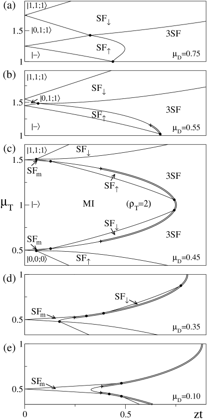
Figure 2: Evolution of the mean field phase diagram with $\mu_{\rm D}$, corresponding to vertical scans through Fig. 1(a). We set $\epsilon_{\uparrow}=\epsilon_{\downarrow}=1$, $\epsilon_{m}=2$, $g=1$, $U=V=0$, $t_{\uparrow}=t_{\downarrow}=t$, and $t_{m}=t/2$. We indicate the one-component up, down and molecular superfluids, by ${\rm SF}_{\uparrow}$, ${\rm SF}_{\downarrow}$ and ${\rm SF}_{m}$, while MI denotes a Mott insulator. Phase 3SF has all three components superfluid. We denote first order (continuous) transitions by double (single) lines. Junctions between phases are indicated by a dot, and the termination of first order lines by a cross.

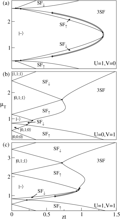
Figure 3: Mean field phase diagram in the presence of interactions, $U$ and $V$. We set $\epsilon_{\uparrow}=\epsilon_{\downarrow}=1$, $\epsilon_{m}=2$, $g=1$, $t_{\uparrow}=t_{\downarrow}=t$, $t_{m}=t/2$ and $\mu_{\rm D}=0.45$ as in Fig. 2(c), and consider the effects of $U$ and $V$ in turn. (a) $U=1$, $V=0$, showing the increase in extent of the $|-\rangle$ Mott lobe. (b) $U=0$, $V=1$, showing the appearance of asymmetry. (c) $U=1$, $V=1$ showing the combined effect of both interactions. The characteristic phases and phase transitions mirror those seen in the $U=V=0$ limit shown in Fig. 2.

As discussed in Ref. Bhaseen:Feshising , in elucidating the zero temperature phase diagram the zero hopping limit provides a useful anchor point. In particular, the topology of the zero hopping phase diagram depends on the Hamiltonian parameters via the energy difference between proximate phases; see Fig. 1. In this respect it is convenient to define the energy gap, $\Delta_{-}\equiv E(0,0;0)-E_{-}$, between the vacuum state and the second Mott lobe, evaluated at the intersection point $E(1,0;0)=E(0,1;0)=E(0,0;0)$, where we label the energies $E(n_{\downarrow},n_{\uparrow};n_{m})$ in the occupation basis. Similarly, we define $\Delta_{+}\equiv E_{-}-E(1,1;1)$, between the second and upper Mott lobes, where $E(1,0;1)=E(0,1;1)=E_{-}$. This yields $\Delta_{\pm}=\sqrt{g^{2}+(h/2)^{2}}-V\pm h/2$, where $h\equiv\epsilon_{m}-\epsilon_{\downarrow}-\epsilon_{\uparrow}-V$. One obtains the structure shown in Fig. 1(a) for $\Delta_{\pm}>0$, (b) for $\Delta_{+}>0$ and $\Delta_{-}<0$, (c) for $\Delta_{\pm}<0$, and (d) for $\Delta_{+}<0$ and $\Delta_{-}>0$.

For simplicity, we begin with the parameters used in Fig. 1(a), where $U=V=0$. Since we include Feshbach resonant interactions, $g$, this limit captures many of the principal features and phases of the interacting problem, including the presence of Mott states. We will incorporate the effects of finite $U$ and $V$ in the subsequent discussion. The mean field phase diagram is obtained by minimizing the effective Hamiltonian

$$H=H_{0}-\sum_{\alpha}zt_{\alpha}\left(a_{\alpha}^{\dagger}\phi_{\alpha}+\phi_{\alpha}^{\ast}a_{\alpha}-|\phi_{\alpha}|^{2}\right),$$ (3)

where $H_{0}$ is the single site zero hopping contribution to (1), $z$ is the coordination, and $\phi_{\alpha}\equiv\langle a_{i\alpha}\rangle$; see Fig. 2. The phase diagram is symmetric under $\mu_{\rm T}\rightarrow 2-\mu_{\rm T}$ due to invariance of the Hamiltonian (1) under particle-hole and spin flip operations, $a_{\alpha}\leftrightarrow a_{\alpha}^{\dagger}$, $\mu_{\rm T}\rightarrow\epsilon_{m}+U-\mu_{\rm T}$, $a_{\downarrow}\leftrightarrow a_{\uparrow}$, when $t_{\downarrow}=t_{\uparrow}$ and $h=0$; this extends the “top-bottom” symmetry in Fig. 1(a). Likewise, the system is invariant under $\mu_{\rm D}\rightarrow\epsilon_{\uparrow}-\epsilon_{\downarrow}-\mu_{\rm D}$, $a_{\downarrow}\leftrightarrow a_{\uparrow}$ and $t_{\downarrow}\leftrightarrow t_{\uparrow}$, which extends the “left-right” symmetry in Fig. 1. The phase diagram has a rich structure and exhibits distinct Mott insulators, single component atomic and molecular condensates, and a phase with all three species superfluid. However, two-component superfluids are absent due to the structure of the Feshbach term Bhaseen:Feshising ; Zhou:PS . The main panel shown in Fig. 2(c) also displays an intricate network of continuous quantum phase transitions, quantum critical points and first order phase transitions, where the latter are inferred by discontinuities in the order parameters and derivatives of the ground state energy. In particular, the first order segments shroud the second Mott lobe and overextend beyond the junctions of the proximate superfluid phases. Similar features also emerge in the two-component Bose–Hubbard model in the absence of Feshbach interactions Kuklov:Commens . As may be seen by tracking the evolution with $\mu_{\rm D}$, these first order segments emerge from an underlying tetracritical point, as shown in panels (a) and (b). In a similar way, the tetracritical points shown in Fig. 2(c) may bifurcate into segments connected by first order transitions as shown in panels (d) and (e). As we shall discuss in Sec. 8, the presence and transmutation of these elementary critical points and first order segments may be seen from a reduced two-component Landau theory. Before embarking on this discussion, let us note that these principal features also emerge for non-vanishing $U$ and $V$, as shown in Fig. 3. Although finite interactions induce quantitative distortions of the phase diagram depicted in Fig. 2, the characteristic phases and phase transitions are nonetheless present in the $U=V=0$ limit.

IV Landau Theory

To understand the structure of the mean field phase diagram we develop a Landau theory description. The eigenenergies of the effective single site Hamiltonian (3) may be calculated by treating the off-diagonal hopping contribution as a perturbation,

$${\mathcal{V}}=-\sum_{\alpha}zt_{\alpha}(a^{\dagger}_{\alpha}\phi_{\alpha}+\text{h.c.}),$$ (4)

where $\alpha=\downarrow,\uparrow,m$. In principle, this may be performed to arbitrary order using the general formalism in Ref. Messiah:QM . To illustrate the observed topology it is sufficient to obtain the appropriate eigenenergy to fourth order

$$\begin{split}&E_{r}=E^{0}_{r}+\langle r|{\mathcal{V}}S^{1}_{r}{\mathcal{V}}|r\rangle+\langle r|{\mathcal{V}}S^{1}_{r}{\mathcal{V}}S^{1}_{r}{\mathcal{V}}|r\rangle\\ &+\langle r|{\mathcal{V}}S^{1}_{r}{\mathcal{V}}S^{1}_{r}{\mathcal{V}}S^{1}_{r}{\mathcal{V}}|r\rangle-\langle r|{\mathcal{V}}S^{1}_{r}{\mathcal{V}}|r\rangle\langle r|{\mathcal{V}}S^{2}_{r}{\mathcal{V}}|r\rangle+\dots,\end{split}$$ (5)

where $r$ labels the zero hopping Mott state, and the operator $S^{k}_{r}=\sum_{n\neq r}|n\rangle\langle n|/(E^{0}_{r}-E^{0}_{n})^{k}$ is introduced Messiah:QM . The expansion (5) takes on a simplified form due to the off-diagonal nature of the perturbation. One obtains

$$\begin{split}E=E_{0}&+\frac{1}{2}\sum_{\alpha}m_{\alpha}|\phi_{\alpha}|^{2}+\frac{\gamma}{2}\left(\phi^{*}_{m}\phi_{\uparrow}\phi_{\downarrow}+\text{h.c.}\right)\\ &+\frac{1}{4}\sum_{\alpha\beta}\lambda_{\alpha\beta}|\phi_{\alpha}|^{2}|\phi_{\beta}|^{2}+\mathcal{O}(\phi^{6}),\end{split}$$ (6)

where the explicit parameters, but not the overall structure, depend on the unperturbed Mott state. The transition to the one-component superfluids is determined by the vanishing of the quadratic mass terms; expressions for these coefficients are given in App. A. The function (6) is minimized when $\arg(\gamma\phi^{*}_{m}\phi_{\downarrow}\phi_{\uparrow})=\pi$, and without loss of generality we may take the fields to be real. To see how a Landau theory of this type gives rise to the observed evolution of the tetracritical points we consider the situation where one of the fields is massive with $m\gg 0$. Replacing this field by its saddle point solution one obtains the energy in terms of the two remaining fields. As a concrete example let us consider the vicinity of the lower tetracritical point shown in Fig. 2(c), where $m_{\downarrow}\gg 0$. The value of $\phi_{\downarrow}$ which minimizes the energy is given by

$$\begin{split}0=\frac{\partial E}{\partial\phi_{\downarrow}}&=m_{\downarrow}\phi_{\downarrow}+\gamma\phi_{m}\phi_{\uparrow}+\lambda_{\downarrow\downarrow}\phi_{\downarrow}^{3}\\ &+\lambda_{\downarrow\uparrow}\phi_{\downarrow}\phi_{\uparrow}^{2}+\lambda_{\downarrow m}\phi_{\downarrow}\phi_{m}^{2}.\end{split}$$ (7)

Taking $\phi_{\downarrow}=-\gamma\phi_{m}\phi_{\uparrow}/m_{\downarrow}+\mathcal{O}(\phi^{4})$ we obtain a reduced two-component Landau theory

$$E=E_{0}+\frac{1}{2}\sum_{\alpha}m_{\alpha}\phi_{\alpha}^{2}+\frac{1}{4}\sum_{\alpha\beta}\Lambda_{\alpha\beta}\phi_{\alpha}^{2}\phi_{\beta}^{2}+\mathcal{O}(\phi^{6}),$$ (8)

where $\alpha,\beta=\uparrow,m$, and the interspecies density-density interaction has been renormalized to $\Lambda_{\uparrow m}=\lambda_{\uparrow m}-\gamma^{2}/m_{\downarrow}$ whilst $\Lambda_{\alpha\alpha}=\lambda_{\alpha\alpha}$ remains unchanged. The behavior of this Landau theory is governed by the sign and magnitude of $\Lambda_{\uparrow m}$ Chaikin:Book .

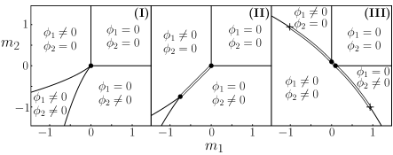
Figure 4: Topologies of the reduced Landau theory (8) with $\alpha,\beta\equiv 1,2$ and a term $(\phi_{1}^{6}+\phi_{2}^{6})/6$ added for stability. We set $\Lambda_{11}=\Lambda_{22}=1$ and consider the evolution with $\Lambda_{12}$. We denote first order (continuous) transitions by double (single) lines. Junctions between phases are indicated by a dot, and the termination of first order lines by a cross. (I) $\Lambda_{12}^{2}<\Lambda_{11}\Lambda_{22}$: tetracritical point for $\Lambda_{12}=0.8$. (II) $\Lambda_{12}>\sqrt{\Lambda_{11}\Lambda_{22}}$: first order transition between one-component condensates for $\Lambda_{12}=1.5$. (III) $\Lambda_{12}<-\sqrt{\Lambda_{11}\Lambda_{22}}$: first order transition with condensation of both order parameters for $\Lambda_{12}=-1.5$.

There are three distinct cases to consider as illustrated in Fig. 4; (I) if $\Lambda_{\uparrow\uparrow}\Lambda_{mm}>\Lambda^{2}_{\uparrow m}$ this describes a tetracritical point; (II) if $\Lambda_{\uparrow m}>\sqrt{\Lambda_{\uparrow\uparrow}\Lambda_{mm}}$ then there is a first order transition between the two single component superfluids; (III) if $\Lambda_{\uparrow m}<-\sqrt{\Lambda_{\uparrow\uparrow}\Lambda_{mm}}$ then the system is unstable at fourth order indicating the presence of a first order transition to condensation of both order parameters. For the parameters used in Fig. 2 we find explicit examples of types (I) and (III); see Figs. 5 and 6.

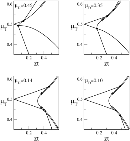
Figure 5: Magnified portion of the lower left region of Fig. 2 showing the underlying tetracritical points as $\mu_{\rm D}$ is varied. The lower and middle tetracritical points bifurcate at $\mu_{\rm D}\approx 0.203$ and $\mu_{\rm D}\approx 0.445$ respectively. The former corresponds to the reduced Landau theory criterion $\Lambda_{\uparrow m}=-\sqrt{\Lambda_{\uparrow\uparrow}\Lambda_{mm}}$ obtained by saddle point elimination of $\phi_{\downarrow}$ in the perturbation expansion around the vacuum state, $|0,0;0\rangle$. The latter corresponds to $\Lambda_{\downarrow m}=-\sqrt{\Lambda_{\downarrow\downarrow}\Lambda_{mm}}$ after eliminating $\phi_{\uparrow}$ in the perturbation expansion around the second Mott lobe, $|-\rangle$.

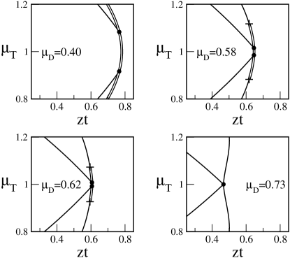
Figure 6: Magnified portion of the second lobe tip in Fig. 2 showing the retreat of the first order transitions and the emergence of a tetracritical point at $\mu_{\rm D}\approx 0.715$. This is given by the reduced Landau theory criterion, $\Lambda_{\uparrow\downarrow}=-\sqrt{\Lambda_{\uparrow\uparrow}\Lambda_{\downarrow\downarrow}}$, obtained after saddle point elimination of $\phi_{m}$ in perturbation theory around the second Mott lobe, $|-\rangle$.

At the lower tetracritical point in Fig. 2(c), where $m_{\uparrow}=m_{m}=0$, the Landau coefficients are given by $\Lambda_{\uparrow\uparrow}=4\tilde{\epsilon}_{\uparrow}$,

$$\Lambda_{mm}=\frac{4[g^{2}-\tilde{\epsilon}_{m}({\tilde{\epsilon}}_{m}-h)]}{h-\tilde{\epsilon}_{m}}\left[\frac{g^{4}+g^{2}(h-\tilde{\epsilon}_{m})^{2}}{(h-2\tilde{\epsilon}_{m})(h-\tilde{\epsilon}_{m})^{3}}+1\right],$$ (9)

and

$$\Lambda_{\uparrow m}=-\frac{2g^{2}}{\tilde{\epsilon}_{\downarrow}}\left[\frac{g^{2}\tilde{\epsilon}_{\downarrow}+{\mathcal{E}}(\tilde{\epsilon}^{2}_{\uparrow}-\tilde{\epsilon}_{\downarrow}^{2}-2\tilde{\epsilon}_{\downarrow}\tilde{\epsilon}_{\uparrow})}{{\mathcal{E}}(\tilde{\epsilon}_{\uparrow}+\tilde{\epsilon}_{\downarrow})^{2}}+\frac{\tilde{\epsilon}_{\uparrow}}{\tilde{\epsilon}_{\downarrow}-\tilde{\epsilon}_{\uparrow}}\right],$$ (10)

where $\mu_{\rm T}=(\epsilon_{\downarrow}+\epsilon_{\uparrow})/2+(\nu-\sqrt{3g^{2}+\nu^{2}})/3$ for $2t_{m}=t_{\downarrow}=t_{\uparrow}=t$, $\nu\equiv h+(\tilde{\epsilon}_{\uparrow}-\tilde{\epsilon}_{\downarrow})/4$ and $\mathcal{E}\equiv\tilde{\epsilon}_{\uparrow}+\tilde{\epsilon}_{m}$. Setting $h=0$ as appropriate for Fig. 2, the bifurcation condition $\Lambda_{\uparrow m}=-\sqrt{\Lambda_{\uparrow\uparrow}\Lambda_{mm}}$ yields $\mu_{\rm D}\approx 0.203g+(\epsilon_{\uparrow}-\epsilon_{\downarrow})/2$. This is in quantitative agreement with the bifurcation point shown in Figs. 2 and 5, where $g=1$. In a similar fashion, for the parameters used in Fig. 2, the $|-\rangle$ lobe tetracritical points bifurcate at $\mu_{\rm D}\approx 0.445$ and $\mu_{\rm D}=(4/\sqrt{7}-1)^{1/2}\approx 0.715$; see Figs. 5 and 6.

V Magnetic Description

Having discussed the phase diagram we turn our attention to the Mott state with total density $\rho_{\rm T}=2$. This reveals Ising transitions in both the heteronuclear and homonuclear lattice problems Bhaseen:Feshising . To explore this second Mott lobe, where the Feshbach term is operative, we adopt a magnetic description. With a pair of atoms or a molecule at each site, we introduce effective spins $|\!\Downarrow\rangle\equiv|1,1;0\rangle$, $|\!\Uparrow\rangle\equiv|0,0;1\rangle$; see Fig. 7. The operators

$$S^{+}=a_{m}^{\dagger}a_{\uparrow}a_{\downarrow},\quad S^{-}=a_{\downarrow}^{\dagger}a_{\uparrow}^{\dagger}a_{m},\quad S^{z}=\frac{1}{2}\left(n_{m}-n_{\downarrow}n_{\uparrow}\right)$$ (11)

or equally $S^{z}=[n_{m}-(n_{\downarrow}+n_{\uparrow})/2]/2$, form a representation of ${\rm su}(2)$ on this reduced Hilbert space. Although the spin representation (11) contains three bosons it is closely related to the more familiar Schwinger construction Auerbach:Interacting . Deep within the Mott phase we perform a strong coupling $t/U$ expansion Duan:Control :

$$H=J\sum_{\langle ij\rangle}S_{i}^{z}S_{j}^{z}+\sum_{i}\left(hS_{i}^{z}+\Gamma S_{i}^{x}\right),$$ (12)

where $\Gamma=2g$, $h=\epsilon_{m}-\epsilon_{\downarrow}-\epsilon_{\uparrow}-V$, and the exchange interaction is given by

$$J=2\left(\frac{t_{\downarrow}^{2}+t_{\uparrow}^{2}}{U-V}+\frac{t_{m}^{2}}{2U}\right).$$ (13)

Here we focus on the antiferromagnetic case with $J>0$. In writing (12) we have omitted the constant, $\tilde{\epsilon}_{m}-h/2-Jz/8$ per site which is necessary for quantitative comparisons; see App. B. More generally, in the presence of asymmetry between $U_{m\uparrow}$ and $U_{m\downarrow}$

$$J=2\left(\frac{t_{\downarrow}^{2}}{U_{m\downarrow}-U_{\uparrow\downarrow}}+\frac{t_{\uparrow}^{2}}{U_{m\uparrow}-U_{\uparrow\downarrow}}+\frac{t_{m}^{2}}{U_{m\downarrow}+U_{m\uparrow}}\right).$$ (14)

The structure of this exchange is readily seen from the energy cost for each individual hopping process in second order perturbation theory. The Hamiltonian (12) takes the form of a quantum Ising model in a longitudinal and transverse field. The longitudinal field, $h$, reflects the energetic asymmetry between a molecule $|\!\!\Uparrow\rangle$, and a pair of atoms $|\!\!\Downarrow\rangle$. The transverse field, $\Gamma\equiv 2g$, encodes Feshbach conversion and induces quantum fluctuations in the ground state; see Fig. 7. In particular, in one dimension and with $h=0$, the model (12) is exactly solvable by fermionization. It exhibits a quantum phase transition at $\Gamma=J/2$ from an ordered to disordered phase Lieb:Two ; Schultz:2D ; Pfeuty:TFI . For $h\neq 0$, the location of this transition is modified; see for example Ref. Ovchinnikov:Mixed .

Figure 7: Schematic representation of the second Mott lobe with $\rho_{\rm T}=2$ showing the presence of a pair of atoms $\Downarrow$ or a molecule $\Uparrow$ at each site. XY exchange involves interchanging a molecule and a pair of atoms, and is suppressed relative to the Ising interaction for small hoppings.

VI Numerical Simulations

The model (12) plays an important role in quantum magnetism and quantum phase transitions Sondhi:Continuous ; Sachdev:QPT . To verify this realization in our bosonic model (1), we perform exact diagonalization on the 1D quantum system (1) with periodic boundary conditions, at zero temperature. The large Hilbert space $\propto 2^{3N}$ of the multicomponent system under consideration restricts our simulations to $N\leq 8$ sites. In Sec. VI.1 we present results for the overall phase diagram in the grand canonical ensemble (allowing all possible states) for $N=6$ sites, before moving on to a detailed canonical ensemble study (allowing only states with fixed total density $\rho_{\rm T}=2$) of the Ising quantum phase transition in Sec. VI.2. Comparing directly to results for the Ising model at a given system size provides a good understanding of finite-size effects in the bosonic problem.

VI.1 Grand Canonical Phase Diagram

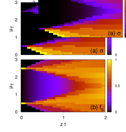
Figure 8: (Color online) (a) Density fluctuations and (b) superfluid fraction for the 1D bosonic model (1) obtained by exact diagonalization for $N=6$ sites. We set $\epsilon_{\downarrow}=\epsilon_{\uparrow}=1$, $\epsilon_{m}=2$, $U=1$, $V=0$, $t=t_{\downarrow}=t_{\uparrow}=2t_{m}$ and $\mu_{\rm D}=0.45$. The extent of the Mott lobes is in good agreement with the mean field predictions in Fig. 3(a). The system sizes are insufficient to resolve the quantum phase transitions between the distinct superfluids shown in Figs. 2 and 3.

In Fig. 8 we present results for the fluctuations in the total density, $\sigma=\sqrt{\langle n_{\rm T}^{2}\rangle-\langle n_{\rm T}\rangle^{2}}$ where $n_{\text{T}}=\sum_{\alpha}n_{i\alpha}$ for an arbitrary site $i$, and the total superfluid fraction

$$f_{\text{s}}=\frac{N}{\sum_{\alpha}t_{\alpha}\langle n_{\alpha}\rangle}\frac{E_{\rm gs}(\Theta)-E_{\rm gs}(0)}{\Theta^{2}}\,.$$ (15)

Here we impose a phase twist $\Theta\ll\pi$ and calculate the change in the ground state energy $E_{\rm gs}(\Theta)$ Roth:Twocolor ; Silver:BHC . These key observables show the onset of superfluidity, and the results are in good qualitative agreement with each other, and with the mean field phase diagram shown in Fig. 3(a). As found in the single component Bose–Hubbard model Fisher:Bosonloc , the Mott lobes develop sharpened tips due to enhanced fluctuations in one dimension Kuhner:Phases ; Kuhner:1DBH . However here, the Mott lobe remains symmetric around the mid-point due to the symmetry of the Hamiltonian (1) under particle-hole and spin flip operations, $a_{\alpha}\leftrightarrow a_{\alpha}^{\dagger}$, $\mu_{\rm T}\rightarrow\epsilon_{m}+U-\mu_{\rm T}$, $a_{\downarrow}\leftrightarrow a_{\uparrow}$, for our chosen parameters with $t_{\downarrow}=t_{\uparrow}$ and $h=0$. The system sizes accessible by exact diagonalization are insufficient to resolve the quantum phase transitions between the distinct superfluids shown in Figs. 2 and 3. However, as we will demonstrate in Sec. VI.2, they provide compelling evidence for the magnetic structure of the Mott phases Bhaseen:Feshising .

VI.2 Ising Transition in the Second Mott Lobe

To employ greater system sizes we switch to the canonical ensemble with fixed density, $\rho_{\rm T}=2$. To study the Ising transition we work in the region of small hopping parameters,

Figure 9: (a) Pseudo staggered magnetization, $m$, versus $\Gamma=2g$, obtained from exact diagonalization of the 1D bosonic model (1) for different system sizes, $N$, at density $\rho_{\rm T}=2$. We take $\epsilon_{\downarrow}=\epsilon_{\uparrow}=1$, $\epsilon_{m}=2$ (corresponding to $h=0$), $U=1$, $V=0$ and set $t=t_{\downarrow}=t_{\uparrow}=2t_{m}=0.01$ corresponding to $J=17t^{2}/4$. (b) Finite size rescaling of $mN^{\beta}$ versus $\Gamma=2g$ showing the presence of the Ising quantum phase transition at $\Gamma=\Gamma_{\text{c}}\approx 2.08\times 10^{-4}$ and the critical exponent $\beta=1/8$ of the 2D classical Ising model. The critical coupling $\Gamma_{c}\approx 0.49J$ is close to the small hopping Ising result, $\Gamma_{c}=J/2$. (c) Scaling collapse as a function of $(\Gamma-\Gamma_{\text{c}})N^{1/\nu}$ corresponding to $\nu=1$.

and begin with $h=0$ before exploring finite fields. Due to the absence of spontaneous symmetry breaking in finite systems, the staggered magnetization vanishes in the absence of an applied staggered field. In view of this we focused our previous numerical investigation Bhaseen:Feshising on the pseudo staggered magnetization, $m\equiv\langle|\sum_{i}(-1)^{i}S_{i}^{z}|\rangle/N$ Um:FiniteTFI , where $S_{i}^{z}=\left[n_{im}-(n_{i\uparrow}+n_{i\downarrow})/2\right]/2$ and additional modulus signs are incorporated. As shown in Fig. 9(a), this quantity is rendered finite. Adopting the finite-size scaling form, $m=N^{-\beta/\nu}\bar{m}\left[(\Gamma-\Gamma_{\text{c}})N^{1/\nu}\right]$ Um:FiniteTFI , we plot $mN^{1/8}$ versus $g$ for different system sizes, $N$, in Fig. 9(b). The curves cross close to the critical coupling, $\Gamma_{\text{c}}=J/2$, of the purely transverse field Ising model. Moreover, the scaling collapse shown in Fig. 9(c) is consistent with the critical exponents $\beta=1/8$ and $\nu=1$ for the 2D classical model. In spite of this evident success, it is clearly desirable to examine this transition in direct physical observables, and we turn our attention to this below. In particular, we establish a direct connection with analytical results and confirm additional Ising critical exponents.

As shown in Fig. 10, the correlation length exponent, $\nu=1$, also follows directly from the gap data. Here we plot $(\Delta/J)N^{\nu}$ versus $\Gamma=2g$, where $\Delta\equiv E_{\rm ex}-E_{\rm gs}$ is the energy gap between the first excited state and the ground state. As indicated in Fig. 10(d),

Figure 10: (a) Dimensionless energy gap $\Delta/J$ versus $\Gamma=2g$ obtained by exact diagonalization of the 1D bosonic Hamiltonian (1) for different system sizes, $N$. We set $\epsilon_{\downarrow}=\epsilon_{\uparrow}=1$, $\epsilon_{m}=2$, $U=1$, $V=0$, $t=t_{\downarrow}=t_{\uparrow}=2t_{m}=0.01$. (b) Scaled energy gap $(\Delta/J)N^{\nu}$ versus $\Gamma=2g$ showing the presence of the Ising quantum phase transition at the numerically extracted value, $\Gamma_{\text{c}}\approx 2.08\times 10^{-4}$, and the correlation length exponent $\nu=1$. (c) Scaling collapse as a function of $(\Gamma-\Gamma_{\text{c}})N^{1/\nu}$ corresponding to $\nu=1$. (d) The numerically extracted critical coupling, $\Gamma_{\text{c}}\approx 2.08\times 10^{-4}$, obtained from the crossing point in Fig. 10 (b) is consistent with the gap closing in the thermodynamic limit, $N\rightarrow\infty$. We set $\Gamma$ equal to multiples of $J/2$ (or the numerically extracted bosonic coupling, $\Gamma_{\text{c}}$) for the Ising (bosonic) model.

Figure 11: (a) Staggered magnetic susceptibility obtained by exact diagonalization of the 1D bosonic Hamiltonian (1) revealing the Ising quantum phase transition at $\Gamma_{\text{c}}\approx 2.08\times 10^{-4}$, and the critical exponent $\gamma=7/4$. We set $\epsilon_{\downarrow}=\epsilon_{\uparrow}=1$, $\epsilon_{m}=2$, $U=1$, $V=0$, $t=t_{\downarrow}=t_{\uparrow}=2t_{m}=0.01$. (b) Scaling collapse showing $\nu=1$. (c) The transverse magnetic susceptibility, $\chi_{\perp}$, plays an analogous role to the specific heat capacity of the 2D classical Ising model. (d) The logarithmic divergence at the critical point yields $\alpha=0$ Um:FiniteTFI . (e) $\log(m_{\text{st}})$ versus $\log(h_{\text{st}}/J)$ to extract the exponent $\delta=15$ for the bosonic model (1) using $m_{\text{st}}\sim h_{\rm st}^{1/\delta}$ for $\Gamma=\Gamma_{\text{c}}\approx 2.08\times 10^{-4}$.

the values of the gap are also in very good quantitative agreement with finite-size simulations of the Ising model.

In a similar fashion we obtain the exponent, $\gamma=7/4$, from the magnetic susceptibility $\chi=\left.\partial m_{\rm st}/\partial h_{\rm st}\right|_{h\rightarrow 0^{+}}$, where $m_{\rm st}\equiv\langle\sum_{i}(-1)^{i}S_{i}^{z}\rangle/N$ and $h_{\rm st}$ is a staggered magnetic field applied to the bosonic Hamiltonian (1), $\Delta H=-h_{\rm st}\sum_{i}(-1)^{i}S_{i}^{z}$; see Figs. 11(a) and (b). A significant advantage of this somewhat more involved procedure is that the staggered magnetic field couples directly to the genuine order parameter, $m_{\text{st}}$, without the need for modification. Likewise, we compute the transverse susceptibility, $\chi_{\perp}=\partial m_{\perp}/\partial\Gamma$, where $m_{\perp}=\sum_{i}\langle S_{i}^{x}\rangle/N$ is the transverse magnetization. Since the transverse field acts to disorder the system, this plays a similar role to the specific heat capacity of the 2D classical Ising model Um:FiniteTFI . The dependence shown in Fig. 11(d) is consistent with the Ising critical exponent $\alpha=0$. At criticality, the relation, $m_{\text{st}}\sim h_{\text{st}}^{1/\delta}$, is also furnished with $\delta=15$ as shown in Fig. 11(e).

All of the above diagnostics confirm the consistency of the measured Ising critical point Bhaseen:Feshising , and we may track this transition within the Mott lobe. The results in Fig. 12 show clear Ising behavior at small hoppings corresponding to $\Gamma_{\text{c}}\approx J/2$.

Figure 12: Ising quantum phase transition in the bosonic model (1) showing the emergence of the critical line, $\Gamma_{c}=J/2$, in the regime of small hoppings. We set $\epsilon_{\downarrow}=\epsilon_{\uparrow}=1$, $\epsilon_{m}=2$, $U=1$, $V=0$, $t=t_{\downarrow}=t_{\uparrow}=2t_{m}$ and vary the hopping, $t$, corresponding to different values of $J=17t^{2}/4$.

With increasing hopping the boundary peels away from this linear slope and we find $\Gamma_{\text{c}}<J/2$. Additionally, enhanced finite-size effects result in slightly different estimates of $\Gamma_{\text{c}}$ from $m$, $\Delta$ and $\chi$; see Fig. 12. This will be explored in future density matrix renormalization group (DMRG) work Ejima:inprep .

As shown in Fig. 13 (a), the results obtained for $N=8$ sites are in good agreement with exact results pertaining to the thermodynamic limit of the quantum Ising model for both the ground-state energy density Pfeuty:TFI

$$e_{\infty}=-\frac{1}{4\pi}\int_{0}^{\pi}dk\sqrt{4\Gamma^{2}+J^{2}+4\Gamma J\cos k},$$ (16)

and the transverse magnetization Pfeuty:TFI ; Hieida:Reentrant

$$\langle S_{i}^{x}\rangle=-\int_{0}^{\pi}\frac{dk}{2\pi}\frac{2\Gamma+J\cos k}{\sqrt{4\Gamma^{2}+J^{2}+4\Gamma J\cos k}}.$$ (17)

In this comparison we define $E_{\rm gs}^{\prime}\equiv E_{\rm gs}-({\tilde{\epsilon}}_{m}-h/2-Jz/8)N$ for the bosonic system (1) in order to take into account the constant offset in the mapping (12).

Figure 13: Comparison of (a) the shifted ground state energy $E_{\rm gs}^{\prime}\equiv E_{\rm gs}-({\tilde{\epsilon}}_{m}-h/2-Jz/8)N$, and (Inset) transverse magnetization $m_{\perp}=\sum_{i}\langle S_{i}^{x}\rangle$/N of the bosonic model (1) and the exact thermodynamic results (16) and (17) for the Ising model. We set $\epsilon_{\downarrow}=\epsilon_{\uparrow}=1$, $\epsilon_{m}=2$, $U=1$, $V=0$, $t=t_{\downarrow}=t_{\uparrow}=2t_{m}=0.01$. (b) Finite size corrections for $E_{\rm gs}^{\prime}$ of the bosonic model (1), with $\Gamma=\Gamma_{\text{c}}\approx 2.08\times 10^{-4}$. We use the finite size scaling result, $E_{\rm gs}^{\prime}/JN=e_{\infty}^{\prime}/J-\pi c(v/J)/6N^{2}$. The intercept at -0.3164 is in good agreement with the exact Ising result (16) in the thermodynamic limit, $e_{\infty}^{\prime}/J=-1/\pi\approx-0.3183$ when $\Gamma=J/2$. The slope, $-\pi c/12$, yields the central charge, $c\approx 0.52$, where we use the characteristic velocity $v=J/2$. (c) Comparison of the low-energy spectra obtained by exact diagonalization for $N=8$ sites in the bosonic model (1) with the same parameters as used in panel (a) with $\Gamma=2g=2J$, and the Ising model (12) with $J=17t^{2}/4$, $h=0$, and $\Gamma=2J$.

The residual finite size effects may be used to find the central charge of the bosonic system. With periodic boundary conditions the ground state energy depends on the system size, $L=Na$, according to $E_{\rm gs}=e_{\infty}L-\pi cv/6L+\dots$, where $e_{\infty}$ is the ground state energy density in the thermodynamic limit, $v$ is the effective velocity in the linearized low energy dispersion, and $c$ is the central charge Blote:Conformal ; Affleck:Universal ; Cardy:scal . For the 1D Ising model (12), the dispersion relation may be obtained by fermionization Lieb:Two ; Schultz:2D ; Pfeuty:TFI . This yields the characteristic velocity, $v=\left.\partial\varepsilon_{k}/\partial k\right|_{k=0}=J/2$. The recovery of the Ising model central charge, $c=1/2$ BPZ ; Francesco:CFT , is shown in Fig. 13(b). Although the majority of our discussion has been on the ground state properties, and the first excited state, the agreement between the Ising model description and the bosonic Hamiltonian also extends to the low-energy spectrum shown in Fig. 13(c).

Having provided a thorough description of the Ising quantum phase transition in the absence of a magnetic field, let us now consider its effect. In the presence of a finite longitudinal field, $h$, the location of the Ising critical point is modified as shown in Fig. 14(a).

Figure 14: (a) Evolution of the Ising quantum phase transition with the longitudinal field, $h$, in the 1D bosonic model (1). Here $\epsilon_{m}=2+h$ and all other parameters as in Fig. 9. (b) Quadratic correction to the ground state energy for the bosonic Hamiltonian (1) due to a longitudinal magnetic field, $h$, in the vicinity of the $h=0$ Ising critical point. We set $\epsilon_{\downarrow}=\epsilon_{\uparrow}=1$, $\epsilon_{m}=2$, $U=1$, $V=0$, $t=t_{\downarrow}=t_{\uparrow}=2t_{m}=0.01$ and $\Gamma=\Gamma_{\text{c}}\approx 2.08\times 10^{-4}$. The results are close to the theoretical value, $\delta E_{\rm gs}^{(2)}\approx-0.0706h^{2}N$, at $\Gamma=\Gamma_{c}$ Ovchinnikov:Mixed .

The results obtained from the pseudo staggered magnetization, magnetic susceptibility, and gap data are in good agreement with exact diagonalization and DMRG results Ovchinnikov:Mixed for the Ising model. Finite-size effects increase with increasing magnetic field, and for $h/J\gtrsim 0.6$ and $N=4,6,8$, clean scaling is observed for $m$, but not for $\Delta$ and $\chi$. In addition, departures from the $h=0$ critical point yield the expected quadratic dependence of the ground state energy on the longitudinal field, $h$. The relation $\delta E_{\rm gs}^{(2)}=-0.0706h^{2}N$ Ovchinnikov:Mixed ; Muller:Sus is recovered in Fig. 14(b). These results show the persistence of an Ising quantum phase transition in the bosonic model without the need to fine tune to zero magnetic field.

VII Conclusions

In this work we have provided a detailed study of bosonic heteronuclear mixtures with Feshbach resonant pairing in optical lattices. The model displays a rich phase diagram with an intricate network of quantum critical points and phase transitions, and we have anchored this behavior to the predictions of a reduced two-component Landau theory. We have substantiated our previous findings of an Ising quantum phase transition occurring within the second Mott lobe Bhaseen:Feshising by significantly extending the range of physical observables. In particular, we have confirmed the additional Ising critical exponents, $\alpha=0$, $\gamma=7/4$, and $\delta=15$, for the one-dimensional bosonic system. There are many directions for further investigation including the superfluid properties, and studies away from the hardcore limit. Cold atoms in optical lattices may represent ideal systems in which to explore magnetization distributions Lamacraft:OPS and quantum quenches Rossini:Thermal ; Calabrese:Quench in quantum Ising models.

Appendix A Landau Coefficients

To calculate the phase boundaries delimiting the single component superfluids from the Mott lobes it is sufficient to examine where the relevant mass terms change sign. In particular, for the second Mott lobe, $|-\rangle$, we find

$$E_{-}=E_{-}^{0}+\frac{1}{2}\sum_{\nu}m_{\nu}\phi_{\nu}^{2}+\dots$$ (18)

where

$$m_{m}=zt_{m}\left\{1-zt_{m}\frac{\chi(\chi+U)+\frac{h}{2}(\frac{h}{2}-{\tilde{\epsilon}}_{m}-U)}{\chi\left[(\chi+U)^{2}-(\frac{h}{2}-{\tilde{\epsilon}}_{m}-U)^{2}\right]}\right\},$$ (19)

and

$$m_{\uparrow\downarrow}=zt_{\uparrow\downarrow}\left\{1-zt_{\uparrow\downarrow}\frac{\chi(\chi-\beta)+\frac{h}{2}({\tilde{\epsilon}}_{\uparrow\downarrow}+\alpha)}{\chi\left[(\chi-\beta)^{2}-({\tilde{\epsilon}}_{\uparrow\downarrow}+\alpha)^{2}\right]}\right\}.$$ (20)

Here we denote $\chi=\sqrt{g^{2}+(h/2)^{2}}$, $\alpha=h/2+(U+V)/2$ and $\beta=(V-U)/2$. The coefficients for $|0,0;0\rangle$ read

$$m_{\uparrow\downarrow}(0,0;0) =zt_{\uparrow\downarrow}\left(1-\frac{zt_{\uparrow\downarrow}}{\tilde{\epsilon}_{\uparrow\downarrow}}\right),$$ (21)

$$m_{m}(0,0;0) =zt_{m}\left(1-\frac{zt_{m}(h-\tilde{\epsilon}_{m})}{\chi^{2}-(\tilde{\epsilon}_{m}-\frac{h}{2})^{2}}\right),$$ (22)

whilst those pertaining to $|1,0;0\rangle$ read

$$m_{m}(1,0;0) =zt_{m}\left(1-\frac{zt_{m}}{\tilde{\epsilon}_{m}+U}\right),$$ (23)

$$m_{\downarrow}(1,0;0) =zt_{\downarrow}\left(1+\frac{zt_{\downarrow}}{\tilde{\epsilon}_{\downarrow}}\right),$$ (24)

$$m_{\uparrow}(1,0;0) =zt_{\uparrow}\left(1+\frac{h+\tilde{\epsilon}_{\uparrow}+V}{\chi^{2}-(\frac{h}{2}+\tilde{\epsilon}_{\uparrow}+V)^{2}}\right).$$ (25)

The remaining coefficients may be obtained by interchanging particles and holes and ups and downs as appropriate. For example, the coefficients $m_{\alpha}(0,1;0)$ are obtained by interchanging $\downarrow\leftrightarrow\uparrow$ in equations (23) — (25). Likewise, the coefficients $m_{\alpha}(1,1;1)$ are obtained by the particle–hole transformation, $\tilde{\epsilon}_{\uparrow\downarrow}\rightarrow-(\tilde{\epsilon}_{\uparrow\downarrow}+U+V)$ and $\tilde{\epsilon}_{m}\rightarrow-(\tilde{\epsilon}_{m}+2U)$, on equations (21) and (22).

Appendix B Derivation of the Ising Hamiltonian

In this Appendix we derive the effective spin model describing the second Mott lobe of the heteronuclear Hamiltonian. Employing the spin operators as defined in equation (11) and noting the form of the zero hopping eigenstates we may re-write the bosonic Hamiltonian (1) as

$$H=NE_{0}\mathcal{P}_{0}+H^{0}+H^{\prime},$$ (26)

where $N$ is the number of lattice sites,

$$H^{0}=\left(\sum_{i\alpha}\tilde{\epsilon}_{\alpha}n_{i\alpha}+\sum_{i\alpha\alpha^{\prime}}\frac{U_{\alpha\alpha^{\prime}}}{2}:n_{i\alpha}n_{i\alpha^{\prime}}:\right)(1-\mathcal{P}_{0}),$$ (27)

and

$$H^{\prime}=\sum_{i,\sigma=\pm}\sigma\chi|\sigma_{i}\rangle\langle\sigma_{i}|-\sum_{\langle ij\rangle,\alpha}t_{\alpha}(a^{\dagger}_{i\alpha}a_{j\alpha}+\text{h.c.}).$$ (28)

Here, $E_{0}=\tilde{\epsilon}_{m}-h/2$, and $\mathcal{P}_{0}=\prod_{i}|\!\!\Downarrow_{i}\rangle\langle\Downarrow_{i}\!\!|+|\!\!\Uparrow_{i}\rangle\langle\Uparrow_{i}\!\!|$ is the projection operator onto the quasi-degenerate subspace of a molecule or two atoms on each site. The effective Hamiltonian within this subspace is Messiah:QM

$$H_{S}=NE_{0}\mathcal{P}_{0}+\mathcal{P}_{0}H^{\prime}\mathcal{P}_{0}+\mathcal{P}_{0}H^{\prime}{S^{\prime}}^{1}H^{\prime}\mathcal{P}_{0}+\mathcal{O}({H^{\prime}}^{3}),$$ (29)

where ${S^{\prime}}^{1}=\sum_{m\neq\Uparrow,\Downarrow}|m\rangle\langle m|/(NE_{0}-E_{|m\rangle})$. Since only the hopping contribution to $H^{\prime}$ connects this subspace to the other states one immediately finds

$$\begin{split}\mathcal{P}_{0}H^{\prime}\mathcal{P}_{0}&=\mathcal{P}_{0}\sum_{i,\sigma=\pm}\sigma\chi|\sigma_{i}\rangle\langle\sigma_{i}|\mathcal{P}_{0}\\ &=\mathcal{P}_{0}\sum_{i}\left[g(S^{+}_{i}+S^{-}_{i})+hS^{z}_{i}\right]\mathcal{P}_{0}.\end{split}$$ (30)

The only process contributing at second order is a particle hopping to a neighboring site and back:

$$\begin{split}\mathcal{P}_{0}H^{\prime}{S^{\prime}}^{1}H^{\prime}\mathcal{P}_{0}&=\sum_{\alpha,\langle ij\rangle}t^{2}_{\alpha}\mathcal{P}_{0}a^{\dagger}_{i\alpha}a_{j\alpha}{S^{\prime}}^{1}a_{i\alpha}a^{\dagger}_{j\alpha}\mathcal{P}_{0}\\ &\qquad+(i\leftrightarrow j).\end{split}$$ (31)

Noting that

$$a^{\dagger}_{im}a_{jm}\mathcal{P}_{0} =|1,1;1\rangle_{i}|0,0;0\rangle_{j}\langle\Uparrow_{j}\Downarrow_{i}\!|\mathcal{P}_{0},$$ (32)

$$a^{\dagger}_{i\uparrow}a_{j\uparrow}\mathcal{P}_{0} =|0,1;1\rangle_{i}|1,0;0\rangle_{j}\langle\Downarrow_{j}\Uparrow_{i}\!|\mathcal{P}_{0},$$ (33)

$$a^{\dagger}_{i\downarrow}a_{j\downarrow}\mathcal{P}_{0} =|1,0;1\rangle_{i}|0,1;0\rangle_{j}\langle\Downarrow_{j}\Uparrow_{i}\!|\mathcal{P}_{0},$$ (34)

one obtains

$$\begin{split}&\mathcal{P}_{0}H^{\prime}{S^{\prime}}^{1}H^{\prime}\mathcal{P}_{0}=\\ &\mathcal{P}_{0}\sum_{\langle ij\rangle}\left(-\frac{t_{m}^{2}}{2U}+\frac{t_{\downarrow}^{2}+t^{2}_{\downarrow}}{V-U}\right)|\Uparrow_{j}\Downarrow_{i}\rangle\langle\Uparrow_{j}\Downarrow_{i}|\mathcal{P}_{0}+(i\leftrightarrow j),\end{split}$$ (35)

where $U_{m\uparrow}=U_{m\downarrow}=U$ and $U_{\uparrow\downarrow}=V$. Using the identity

$$|\!\Uparrow_{j}\Downarrow_{i}\rangle\langle\Uparrow_{j}\Downarrow_{i}\!|=(1/2+S^{z}_{j})(1/2-S^{z}_{i})$$ (36)

one obtains

$$\begin{split}\mathcal{P}_{0}H^{\prime}{S^{\prime}}^{1}H^{\prime}\mathcal{P}_{0}&=-\mathcal{P}_{0}J\sum_{\langle ij\rangle}\left(\frac{1}{4}-S^{z}_{i}S^{z}_{j}\right)\mathcal{P}_{0},\end{split}$$ (37)

where $J$ is given by equation (13). We conclude that

$$\begin{split}H&=\mathcal{P}_{0}\left[\sum_{i}\left(\tilde{\epsilon}_{m}-\frac{h}{2}-\frac{zJ}{8}\right)+J\sum_{\langle ij\rangle}S^{z}_{i}S^{z}_{j}\right.\\ &\left.\hskip 56.9055pt+\Gamma\sum_{i}S^{x}_{i}+h\sum_{i}S_{i}^{z}\right]\mathcal{P}_{0},\end{split}$$ (38)

as stated in equation (12). In the zero hopping limit the eigenstates of Hamiltonians (1) and (38) coincide, including the mixing induced by the Feshbach coupling.

References

- (1) L. Santos, G. V. Shlyapnikov, P. Zoller, and M. Lewenstein, Phys. Rev. Lett. 85, 1791 (2000)
- (2) M. A. Baranov, Phys. Rep. 464, 71 (2008)
- (3) S. Ospelkaus, K.-K. Ni, D. Wang, M. H. G. de Miranda, B. Neyenhuis, G. Quéméner, P. S. Julienne, J. L. Bohn, D. S. Jin, and J. Ye, Science 327, 853 (2010)
- (4) S. B. Papp and C. E. Wieman, Phys. Rev. Lett. 97, 180404 (2006)
- (5) S. B. Papp, J. M. Pino, and C. E. Wieman, Phys. Rev. Lett. 101, 040402 (2008)
- (6) C. Ticknor, C. A. Regal, D. S. Jin, and J. L. Bohn, Phys. Rev. A 69, 042712 (2004)
- (7) C. Weber, G. Barontini, J. Catani, G. Thalhammer, M. Inguscio, and F. Minardi, Phys. Rev. A 78, 061601(R) (2008)
- (8) G. Thalhammer, G. Barontini, L. D. Sarlo, J. Catani, F. Minardi, and M. Inguscio, Phys. Rev. Lett. 100, 210402 (2008)
- (9) G. Thalhammer, G. Barontini, J. Catani, F. Rabatti, C. Weber, A. Simoni, F. Minardi, and M. Inguscio, New J. Phys. 11, 055044 (2009)
- (10) G. Barontini, C. Weber, F. Rabatti, G. Catani, G. Thalhammer, M. Inguscio, and F. Minardi, Phys. Rev. Lett. 103, 043201 (2009)
- (11) J. Catani, G. Barontini, G. Lamporesi, F. Rabatti, G. Thalhammer, F. Minardi, S. Stringari, and M. Inguscio, Phys. Rev. Lett. 103, 140401 (2009)
- (12) G. Lamporesi, J. Catani, G. Barontini, Y. Nishida, M. Inguscio, and F. Minardi, Phys. Rev. Lett. 104, 153202 (2010)
- (13) A. Simoni, M. Zaccanti, C. D’Errico, M. Fattori, G. Roati, M. Inguscio, and G. Modugno, Phys. Rev. A 77, 052705 (2008)
- (14) K. Pilch, A. D. Lange, A. Prantner, G. Kerner, F. Ferlaino, H.-C. Nägerl, and R. Grimm, Phys. Rev. A 79, 042718 (2009)
- (15) M. J. Bhaseen, A. O. Silver, M. Hohenadler, and B. D. Simons, Phys. Rev. Lett. 103, 265302 (2009)
- (16) L. Zhou, J. Qian, H. Pu, W. Zhang, and H. Y. Ling, Phys. Rev. A 78, 053612 (2008)
- (17) L. Radzihovsky and S. Choi, Phys. Rev. Lett. 103, 095302 (2009)
- (18) E. Timmermans, P. Tommasini, M. Hussein, and A. Kerman, Phys. Rep. 315, 199 (1999)
- (19) L. Radzihovsky, J. Park, and P. B. Weichman, Phys. Rev. Lett. 92, 160402 (2004)
- (20) M. W. J. Romans, R. A. Duine, S. Sachdev, and H. T. C. Stoof, Phys. Rev. Lett. 93, 020405 (2004)
- (21) A. Koetsier, P. Massignan, R. A. Duine, and H. T. C. Stoof, Phys. Rev. A 79, 063609 (2009)
- (22) L. Radzihovsky, P. B. Weichman, and J. I. Park, Ann. Phys. 323, 2376 (2008)
- (23) D. B. M. Dickerscheid, U. Al Khawaja, D. van Oosten, and H. T. C. Stoof, Phys. Rev. A 71, 043604 (2005)
- (24) K. Sengupta and N. Dupuis, Europhys. Lett. 70, 586 (2005)
- (25) V. G. Rousseau and P. J. H. Denteneer, Phys. Rev. Lett 102, 015301 (2009)
- (26) V. G. Rousseau and P. J. H. Denteneer, Phys. Rev. A 77, 013609 (2008)
- (27) A. Kuklov, N. Prokof’ev, and B. Svistunov, Phys. Rev. Lett. 92, 050402 (2004)
- (28) A. Messiah, Quantum Mechanics (Dover, 1999)
- (29) P. M. Chaikin and T. C. Lubensky, Principles of Condensed Matter Physics (Cambridge University Press, 1995)
- (30) A. Auerbach, Interacting Electrons and Quantum Magnetism (Springer, 1994)
- (31) L. M. Duan, E. Demler, and M. D. Lukin, Phys. Rev. Lett. 91, 090402 (2003)
- (32) E. Lieb, T. Schultz, and D. Mattis, Ann. Phys. 16, 407 (1961)
- (33) T. D. Schultz, D. C. Mattis, and E. H. Lieb, Rev. Mod. Phys. 36, 856 (1964)
- (34) P. Pfeuty, Ann. Phys. 57, 79 (1970)
- (35) A. A. Ovchinnikov, D. V. Dmitriev, V. Y. Krivnov, and V. O. Cheranovskii, Phys. Rev. B 68, 214406 (2003)
- (36) S. L. Sondhi, S. M. Girvin, J. P. Carini, and D. Shahar, Rev. Mod. Phys. 69, 315 (1997)
- (37) S. Sachdev, Quantum Phase Transitions (Cambridge University Press, 1999)
- (38) R. Roth and K. Burnett, Phys. Rev. A 68, 023604 (2003)
- (39) A. O. Silver, M. Hohenadler, M. J. Bhaseen, and B. D. Simons, Phys. Rev. A 81, 023617 (2010)
- (40) M. P. A. Fisher, P. B. Weichman, G. Grinstein, and D. S. Fisher, Phys. Rev. B 40, 546 (1989)
- (41) T. D. Kühner and H. Monien, Phys. Rev. B 58, R14741 (1998)
- (42) T. D. Kühner, S. R. White, and H. Monien, Phys. Rev. B 61, 12474 (2000)
- (43) J. Um, S.-I. Lee, and B. J. Kim, J. Korean Phys. Soc. 50, 285 (2007)
- (44) S. Ejima et al, in preparation
- (45) Y. Hieida, K. Okunishi, and Y. Akutsu, Phys. Rev. B 64, 224422 (2001)
- (46) H. W. J. Blöte, J. L. Cardy, and M. P. Nightingale, Phys. Rev. Lett. 56, 742 (1986)
- (47) I. Affleck, Phys. Rev. Lett. 56, 746 (1986)
- (48) J. Cardy, Scaling and Renormalization in Statistical Physics (Cambridge University Press, 1996)
- (49) A. A. Belavin, A. M. Polyakov, and A. B. Zamolodchikov, Nucl. Phys. B241, 333 (1984)
- (50) P. D. Francesco, P. Mathieu, and D. Sénéchal, Conformal Field Theory (Springer, 1997)
- (51) G. Müller and R. E. Shrock, Phys. Rev. B 30, 5254 (1984)
- (52) A. Lamacraft and P. Fendley, Phys. Rev. Lett. 100, 165706 (2008)
- (53) D. Rossini, A. Silva, G. Mussardo, and G. E. Santoro, Phys. Rev. Lett. 102, 127204 (2009)
- (54) P. Calabrese and J. Cardy, Phys. Rev. Lett. 96, 136801 (2006)