Finding and Classifying Critical Points of 2D Vector Fields: A Cell-Oriented Approach Using Group Theory

Abstract

We present a novel approach to finding critical points in cell-wise barycentrically or bilinearly interpolated vector fields on surfaces. The Poincaré index of the critical points is determined by investigating the qualitative behavior of 0-level sets of the interpolants of the vector field components in parameter space using precomputed combinatorial results, thus avoiding the computation of the Jacobian of the vector field at the critical points in order to determine its index. The locations of the critical points within a cell are determined analytically to achieve accurate results. This approach leads to a correct treatment of cases with two first-order critical points or one second-order critical point of bilinearly interpolated vector fields within one cell, which would be missed by examining the linearized field only. We show that for the considered interpolation schemes determining the index of a critical point can be seen as a coloring problem of cell edges. A complete classification of all possible colorings in terms of the types and number of critical points yielded by each coloring is given using computational group theory. We present an efficient algorithm that makes use of these precomputed classifications in order to find and classify critical points in a cell-by-cell fashion. Issues of numerical stability, construction of the topological skeleton, topological simplification, and the statistics of the different types of critical points are also discussed.

Keywords: Vector field topology, interpolation, barycentric interpolation, linear interpolation, bilinear interpolation, level sets, higher-order singularities, computational group theory, colorings.

1 Introduction

The visualization of vector field topology is a problem that arises naturally when studying the qualitative structure of flows that are tangential to some surface. As usual, we use the term surface for a real, smooth 2-manifold (equipped with an atlas consisting of charts), see for example [O’N83] for an introduction to Riemannian Geometry. Having its roots in the theory of dynamical systems, the topological skeleton of a Hamiltonian flow on a surface with isolated critical points consists of these critical points and trajectories (streamlines) of the vector field that lie at the boundary of a hyperbolic sector and connect two of the critical points. Helman and Hesselink [HH90] introduced the concept of the topology of a planar vector field to the visualization community and proposed the following construction scheme: (1) critical points are located, (2) classified, and then (3) trajectories along hyperbolic sectors are traced and connected to their originating and terminating critical points or boundary points. Step (2)—the classification of a critical point—is usually based on the Jacobian of the vector field, see [Per91]. Trajectories of step (3) are typically constructed by solving an ordinary differential equation for particle tracing.

Although a vast body of previous work in the field of flow visualization focuses on the problem of how to extend the method of Helman and Hesselink to vector fields on arbitrary surfaces as well as the second and third step of the above algorithm, not much attention has been paid to the first step. In this paper, we specifically address the identification and classification of critical points in parameter space.

As efficient computer-based visualization algorithms usually work with discrete parametrized versions of the surfaces involved — examples of popular discretization schemes are for example triangulated or quadrangulated versions of the surface — we will in this paper not focus on the well-researched field of how to parametrize a given surface (see [FH05] for a recent survey) but assume that a surface always comes equipped with a globally continuous discrete parametrization that allows a cell-wise (local) barycentric or bilinear interpolation scheme of a vector field tangential to the surface in parameter space.

While this task is rather easy for linear vector fields, the problem setting becomes more interesting for bilinearly interpolated fields. Bilinear interpolation is ubiquitous in scientific visualization because it is popular for widely used uniform or curvilinear grids representing planar or curved surfaces. Since bilinear interpolation is not linear, it can lead to higher-order critical points, which are neglected by often-used linearization approaches.

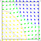
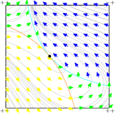
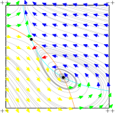
(a)	(b)	(c)

Figure 1: Classification of critical points for three intersection cases for the $0$-level sets of the two vector field components $f_{1}$ (cyan) and $f_{2}$ (orange) of a bilinearly interpolated vector field $\vec{f}=(f_{1},f_{2})^{T}$: (a) no intersection of the level sets, (b) touching of the level sets yielding one critical point, (c) double intersection of the level sets yielding two critical points (one saddle and one non-saddle). The colors of the vector arrows encode the types of characteristic areas as defined in Section 4.2 (green=$++$, yellow=$+-$, blue=$-+$, red=$--$), a set of streamlines is shown in gray, and critical points lying in the intersection set of the two level sets are shown as black dots. Each vertex of a square is marked with $++$, $+-$, $-+$, $--$ according to the sign of $f_{1}$ and $f_{2}$ at that vertex.

In this paper, we introduce a new method that locates and classifies all critical points within piecewise linearly (barycentrically) or bilinearly interpolated two-dimensional grids. Our method determines the index of a critical point without the need to evaluate the Jacobian of the vector field in the critical point in order to determine its Poincaré index. For the case of bilinearly interpolated vector fields, our method is able to detect higher-order critical points and the presence of two first-order critical points within one cell, which, to our knowledge, has not been achieved with the common methods [HH91] for the bilinear interpolation scheme before. Figure 1 shows a corresponding example and illustrates our classification method. Our approach is based on the idea that investigating the qualitative behavior of 0-level sets of the components of the interpolated vector field provides information needed to compute the Poincaré index of a critical point. All qualitatively different possibilities of this behavior and the types of critical points yielded by each possibility are completely classified using the computational group theory tool GAP (Groups, Algorithms, and Programming) [GAP06]. See the enumeration of cases for marching cubes and generic substitope algorithms by Banks et al. [BLS04] for a previous example of an application of computational group theory in the field of scientific visualization. Furthermore, we discuss a cell-based topology simplification method as well as the question of numerical stability. Our approach results in an efficient, accurate, and robust cell-based algorithm for detecting all critical points of barycentrically or bilinearly interpolated 2D vector fields.

The paper is organized as follows. First, we will give a short review of the visualization literature dealing with vector field topology. Then, the theoretical foundations of vector field topology, namely the theory of the qualitative behavior of second-order dynamical systems along with such fundamental notions as those of critical points, separatrices, and the Poincaré index of a critical point are reviewed. Following this, we will present our new approach—first the general framework will be discussed and then applied to two cases: barycentrically and bilinearly interpolated vector fields. Then, we will deal with open issues such as critical points on the boundary of cells and numeric stability followed by a more detailed description of the cell-based algorithm. We will conclude giving results and a short review of our method.

This paper has accompanying material in the form of online resources, namely the GAP programs used in this paper (Online Resource 3) and lists of equivalence classes of colored cells referred to in Theorem 5.3 (Online Resource 1) and Theorem 6.7 (Online Resource 2).

2 Previous Work

Topology-based methods for planar vector fields were first proposed to the visualization community by Helman and Hesselink [HH90], employing methods from the theory of dynamical systems [ALGM73] to planar linear (or linearized) vector fields in order to visualize flow characteristics. Their work has triggered a large body of further research on topology-based flow visualization, an overview of which is given by Post et al. [PVH⁺03] and Scheuermann and Tricoche [ST05].

The case of a planar linear vector field is relatively simple to deal with, but it has a couple of drawbacks, most notably that only first-order critical points can be detected. Much effort has been put into methods to overcome this drawback imposed by the interpolation scheme and to addresses the issue of detecting and processing higher-order critical points of interpolated vector fields, also of vector fields on arbitrary surfaces [LCJK⁺09]. Such higher-order critical points can be found, for example, by using piecewise linear interpolation schemes in combination with a clustering of first-order critical points according to Tricoche et al. [TSH00]. Another example is the work by Theisel [The02], who proposes a method for designing piecewise linear planar vector fields of arbitrary topology. Nonlinear interpolation schemes have been investigated by Scheuermann et al. [SHK⁺97] and Zhang et al. [ZMT06]. Scheuermann et al. [SKMR98] propose a way to approximate higher-order critical points using Clifford algebra. Li et al. [LVRL06] use interpolation schemes based on a polar coordinate representation to detect vector field singularities on a surface.

In contrast to the global variational approach taken in [PP03] in which the authors construct a discrete Hodge decomposition in order to obtain location and type of critical points of vector fields on polyhedral surfaces, our approach is local and cell-oriented. It may thus be easier to implement when a discrete parametrization of the surface is already given and can be used in conjunction with other local, grid-based methods.

3 Theoretical Background

The methods used for extracting vector field topology are founded upon the theory of the qualitative behavior of dynamical systems. Most of the brief review of the essential theory in this section is taken from the books [DLA06, Per91, ALGM73].

3.1 Dynamical Systems

Definition 3.1.

A dynamical system on $E\subset\mathbb{R}^{n}$, an open subset of $\mathbb{R}^{n}$, is a $C^{1}$ map $\vec{\phi}:\mathbb{R}\times E\rightarrow E$, where $\vec{\phi}=\vec{\phi}(t,\vec{x})$ with $t\in\mathbb{R}$, $\vec{x}\in E$, that satisfies

1. $\vec{\phi}(0,\vec{x})=\vec{x}$ $\forall_{\vec{x}\in E}$,

2. $\vec{\phi}(s,\vec{x})\circ\vec{\phi}(t,\vec{x})=\vec{\phi}(s+t,\vec{x})$ $\forall_{\vec{x}\in E,\leavevmode\nobreak\ u,v\in\mathbb{R}}$.

Dynamical systems are closely related to autonomous systems of differential equations. On the one hand, let $E\subset\mathbb{R}^{n}$ be open and let $\vec{f}\in C^{1}(E)$ be Lipschitz continuous on $E$. Then the initial value problem of the autonomous system of differential equations

$$\dot{\vec{x}}=\frac{d\vec{x}}{dt}=\vec{f}(\vec{x}),$$ (3.1)

with $\vec{x}(0)=\vec{x}_{0}$ for any $\vec{x}_{0}\in E$ has a unique solution defined for all $t\in\mathbb{R}$ by virtue of the Picard–Lindelöf theorem. For each initial value $\vec{x}_{0}\in E$ this induces a mapping $\vec{\phi}(t,\vec{x_{0}}):\mathbb{R}\times E\rightarrow E$ referred to as a trajectory of the system (3.1). The mapping $\vec{\phi}$ then lies in $C^{1}(\mathbb{R}\times E)$ and thus is a dynamical system in the sense of Definition 3.1. It is called the dynamical system induced by the system of differential equations (3.1). On the other hand, if $\vec{\phi}(t,\vec{x})$ is a dynamical system on $E\subset\mathbb{R}^{n}$, then

$$\vec{f}(\vec{x})=\frac{d}{dt}\vec{\phi}(t,\vec{x})|_{t=0}$$

defines a $C^{1}$ vector field $f$ on $E$ and for each $\vec{x}_{0}\in E$, $\vec{\phi}(t,\vec{x}_{0})$ is the solution to the initial value problem with $\vec{x}=\vec{x}_{0}$ of (3.1).

3.2 Critical Points

An important concept in the field of dynamical systems is the notion of a critical point:

Definition 3.2.

An equilibrium or critical point $\vec{x_{0}}\in\mathbb{R}^{n}$ of a dynamical system $\vec{\phi}$ is a point where $\vec{\phi}(t,\vec{x_{0}})=\vec{x}_{0}$ $\forall_{t\in\mathbb{R}}$. If the dynamical system is induced by a system of differential equations (3.1), then a critical point $\vec{x}_{0}$ of $\vec{\phi}$ is a point where $\vec{f}(\vec{x_{0}})=\vec{0}$. If the Jacobian $D\vec{f}(\vec{x_{0}})$ has only eigenvalues with nonvanishing real part, $\vec{x_{0}}$ is called a hyperbolic critical point. If $\det D\vec{f}(\vec{x_{0}})\neq 0$, then $\vec{x_{0}}$ is called non-degenerate or first-order critical point. Otherwise it is called degenerate or higher-order critical point.

A system of differential equations can be approximated by its linearization around a critical point $\vec{x_{0}}$ without changing its qualitative behavior if $\vec{x_{0}}$ is a hyperbolic critical point of that system (Hartman-Grobman theorem [Per91]). For planar linear systems, only certain types of critical points can occur and these can be classified in terms of the eigenvalues of the Jacobian as shown in Fig. 2 (here only non-degenerate cases with $\det D\vec{f}(\vec{x_{0}})\neq 0$ are considered).

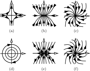
Figure 2: First-order critical points of planar vector fields classified in terms of the eigenvalues $\lambda_{1},\lambda_{2}$ of the Jacobian: (a) saddle ($\Re(\lambda_{1})\Re(\lambda_{2})<0$, $\Im(\lambda_{1})=\Im(\lambda_{2})=0$), (b) attracting node ($\Re(\lambda_{1}),\Re(\lambda_{2})<0$, $\Im(\lambda_{1})=\Im(\lambda_{2})=0$), (c) attracting focus ($\Re(\lambda_{1}),\Re(\lambda_{2})<0$, $\Im(\lambda_{1}),\Im(\lambda_{2})\neq 0$), (d) center ($\Re(\lambda_{1})=\Re(\lambda_{2})=0$, $\Im(\lambda_{1}),\Im(\lambda_{2})\neq 0$), (e) repelling node ($\Re(\lambda_{1}),\Re(\lambda_{2})>0$, $\Im(\lambda_{1})=\Im(\lambda_{2})=0$), (f) repelling focus ($\Re(\lambda_{1}),\Re(\lambda_{2})>0$, $\Im(\lambda_{1}),\Im(\lambda_{2})\neq 0$).

3.3 Poincaré Index of a Critical Point

In order to classify critical points of vector fields one can use the notion of the Poincaré index (or index for short) of a critical point.

Definition 3.3.

Let $\vec{f}=(f_{1},f_{2})^{T}$ be a $C^{1}(E)$ vector field on some open $E\subset\mathbb{R}^{2}$. If $\vec{x_{0}}$ is an isolated critical point of $\vec{f}$ and $\Gamma\subset E$ a Jordan curve such that $\vec{x_{0}}$ is the only critical point of $\vec{f}$ in its interior, then the Poincaré index of $\vec{x_{0}}$ (or index for short) is

$$I_{\vec{f}}(\vec{x_{0}}):=I_{\vec{f}}(\Gamma):=\frac{1}{2\pi}\oint_{\Gamma}d\theta\in\mathbb{Z},$$

with $\theta=\arctan\frac{f_{2}}{f_{1}}$.

It can be shown that isolated first-order critical points (i.e. isolated critical points for which the Jacobian of the vector field in the critical point has no eigenvalue of 0) have a Poincaré index of $\pm$1 and that a saddle has a Poincaré index of $-$1, whereas non-saddles have a Poincaré index of $+$1 (see Fig. 2).

3.4 Topological Equivalence and Sectors

Let us now establish the fundamental notion of topological equivalence of vector fields:

Definition 3.4.

Suppose that $\vec{f}\in C^{1}(E)$ and $\vec{g}\in C^{1}(F)$ with open sets $E,F\subset\mathbb{R}^{n}$. The two autonomous systems of differential equations $\dot{\vec{x}}=\vec{f}(\vec{x})$ and $\dot{\vec{x}}=\vec{g}(\vec{x})$ and thier induced vector fields are said to be topologically equivalent if there exists an orientation preserving homeomorphism that maps trajectories of the first system onto trajectories of the seconds system.

Markus [Mar54] showed that for planar $C^{1}$ systems of differential equations the condition of being topologically equivalent is equivalent to the systems having the same separatrix configurations, where a separatrix of a system (3.1) is a trajectory of (3.1) which is either a critical point, a limit cycle, or a trajectory lying on the boundary of a hyperbolic sector as defined below. This justifies the use of the term vector field topology for the topological skeleton of a vector field consisting of separatrices of that field.

The notion of sectors was first introduced by Poincaré [Poi93] to investigate higher-order critical points of planar systems, and later extended by Bendixon [Ben01] and Andronov [ALGM73]. The idea is that one can describe the qualitative behavior of a planar $C^{1}$ vector field $\vec{f}$ in a suitable neighborhood $N(\vec{x}_{0})$ of an isolated critical point $\vec{x_{0}}$ of $\vec{f}$ in terms of connected regions, so called sectors, which form a partition of $N(\vec{x}_{0})$. Within each sector the trajectories of $f$ exhibit a behavior that is characteristic for this type of sector. It can be shown that there exist three topologically different types of sectors:

Definition 3.5.

A sector of a critical point $\vec{x_{0}}$ can be classified as a hyperbolic, parabolic, or elliptic sector according to its topological structure as shown in Fig. 3.

Figure 3: The three distinct topological sectors of the vector field around an isolated critical point with nonvanishing Jacobian (modulo the operation of reversing the vector field direction): (a) hyperbolic sector (with two separatrices), (b) parabolic sector, (c) elliptic sector.

Tricoche et al. [TSH00] also used the idea of sectors to model higher-order critical points with a piecewise linear interpolation scheme.

3.5 Bifurcation Theory

Bifurcation theory is based on the notion of structural stability of a vector field due to Andronov and Pontryagin [AP37]: if the qualitative behavior of a dynamical system (3.1) does not change for small perturbations of the vector field $\vec{f}$, then that vector field is called structurally stable. If $\vec{f}$ is not structurally stable, the topological skeleton of the vector field changes even under small perturbations of the vector field $\vec{f}$ and $\vec{f}$ is said to be structurally unstable or to lie within the bifurcation set.

The perturbation of the vector field is usually modeled by an additional parameter $\mu\in\mathbb{R}$:

$$\frac{d\vec{x}}{dt}=\vec{f}(\vec{x},\mu).$$ (3.2)

A value of $\mu=\mu_{0}\in\mathbb{R}$ for which the system (3.2) lies in the bifurcation set is called a bifurcation point of (3.2) and $\mu_{0}$ is then called bifurcation value of (3.2).

Bifurcation theory has been studied extensively, see for example the book by Guckenheimer and Holmes [GH90]. It also explains the splitting of higher-order critical points into several nearby first-order critical points: it can be shown that, if a vector field $\vec{f}$ has an isolated critical point $\vec{x_{0}}$ of higher order, there exists a perturbation of $\vec{f}$ such that $\vec{x_{0}}$ splits into several isolated first-order critical points nearby.

4 Classifying Critical Points Without Using the Jacobian

In this section, we show how the Poincaré index of an isolated first-order critical point can be computed by evaluating the sign configuration of the vector field’s components on a finite set of sample points in a neighborhood of the critical point, reminiscent of the marching-cubes classification applied to isosurfaces in scalar fields.

4.1 Setting

From now on let $\vec{f}\in C^{1}(E)$ be a vector field $\vec{f}:E\subset\mathbb{R}^{2}\rightarrow\mathbb{R}^{2}$ defined on an open $E\subset\mathbb{R}^{2}$ such that $\vec{f}$ is Lipschitz continuous on $E$ and only has non-degenerate first-order isolated critical points.

4.2 $\omega$-level sets, Areas of Characteristic Behavior

We introduce the notion of areas of characteristic behavior that will enable us to calculate the index of a critical point.

Lemma 4.1.

Let $\vec{f}=(f_{1},f_{2})^{T}$ be a vector field like in 4.1 and $\vec{x_{0}}\in E$ an isolated first-order critical point of $\vec{f}$, i.e. $\det D\vec{f}(\vec{x_{0}})$
$\neq 0$. Then, $\vec{x_{0}}$ lies in the intersection of the 0-level sets $c_{1}$ and $c_{2}$ of $f_{1}$ and $f_{2}$. Furthermore, there exists an $\epsilon>0$ such that $c_{1}$ and $c_{2}$ are infinitesimally straight lines (i.e. lie infinitesimally close to straight lines) in an $\epsilon$-neighborhood of $\vec{x_{0}}$.

Proof.

By definition, a critical point of $\vec{f}$ has to lie in the intersection set of the 0-level sets of the components of $\vec{f}$. Since $\vec{f}$ is linearizable around $\vec{x_{0}}$, Taylor’s theorem leads to $\vec{f}(\vec{x})\approx\vec{f}(\vec{x_{0}})+D\vec{f}(\vec{x_{0}})(\vec{x}-\vec{x_{0}})$ with $\vec{x}$ in the $\epsilon$-ball $B_{\epsilon}(\vec{x_{0}})$. Since $D\vec{f}(\vec{x_{0}})$ has full rank, the 0-level sets of $D\vec{f}(\vec{x_{0}})$ are straight lines intersecting in $\vec{x_{0}}$. $\square$

Definition 4.2.

Let $\vec{f}=(f_{1},f_{2})^{T}$ be a vector field like in 4.1 and $\vec{x_{0}}\in E$ an isolated first-order critical point of $\vec{f}$. Then for an $\epsilon>0$ the 0-level sets $c_{1}$ of $f_{1}$ and $c_{2}$ of $f_{2}$ partition the $\epsilon$-ball $B_{\epsilon}(\vec{x_{0}})$ of $\vec{x_{0}}$ into four disjoint open subsets $A_{1},\dots,A_{4}$ called areas of characteristic behavior or areas for short.

In each area, the signs of $f_{1}$ and $f_{2}$ do not change, i.e. for arbitrary $1\leq i\leq 4$ and ${\vec{x},\vec{y}\in A_{i}}$ the following holds:

$$f_{j}\neq 0\text{ and }\text{sgn}(f_{j}(\vec{x}))=\text{sgn}(f_{j}(\vec{y}))\text{ for $j=1,2$}.$$

The set of areas $A_{1},\dots,A_{4}$ around a critical point can be seen as an ordered, cyclic sequence of areas according to the order in which they intersect with the boundary of $B_{\epsilon}(\vec{x_{0}})$, as illustrated in Fig. 4. We consider clockwise traversal direction unless otherwise noted.

Since each of the two vector field components can either be positive or negative in one area, there exist four different types of characteristic areas as shown in Fig. 5(a). In the following, areas are written as ordered 2-tuples over the set $\{+,-\}$ or equivalently as elements of the set $\{1,2,3,4\}$, where $1=(+,+)$, $2=(+,-)$, $3=(-,+)$, $4=(-,-)$. Area sequences can then be written as ordered 4-tuples over the set of areas, i.e. as ordered 4-tuples over the set $\{1,\dots,4\}$. Two areas that lie next to each other are called adjacent areas. As $A_{1}$ and $A_{4}$ are adjacent, the indices of the areas in the area sequence are cyclic, i.e. the area sequence $A_{1},\dots,A_{4}$ is glued together at $A_{1}$ and $A_{4}$.

Remark 4.3.

For two adjacent areas $A_{i},A_{i+1}$ of an area sequence with $\vec{x}\in A_{i}$, $\vec{y}\in A_{i+1}$, either

$$\text{sgn}(f_{1}(\vec{x}))\neq\text{sgn}(f_{1}(\vec{y}))\wedge\text{sgn}(f_{2}(\vec{x}))=\text{sgn}(f_{2}(\vec{y}))\text{\leavevmode\nobreak\ \leavevmode\nobreak\ or}$$

$$\text{sgn}(f_{1}(\vec{x}))=\text{sgn}(f_{1}(\vec{y}))\wedge\text{sgn}(f_{2}(\vec{x}))\neq\text{sgn}(f_{2}(\vec{y}))$$

holds, i.e. exactly one component flips its sign for two adjacent areas but not both.

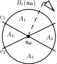
Figure 4: Area sequence ($A_{1},\dots,A_{4}$) around an isolated critical point of a $C^{1}$ vector field $\vec{f}=(f_{1},f_{2})^{T}$ defined by the 0-level sets $c_{1}$ and $c_{2}$ of $f_{1}$ and $f_{2}$. The area sequence of a critical point $\vec{x}_{0}$ can be constructed by walking monotonously around the boundary of an $\epsilon$-ball $B_{\epsilon}(\vec{x}_{0})$ of $\vec{x}_{0}$ starting at an arbitrary position (shown as dashed line above) and collecting the intersection points of $c_{1}$ and $c_{2}$ with $B_{\epsilon}(\vec{x}_{0})$.

4.3 Area Sequence and Types of Critical Points

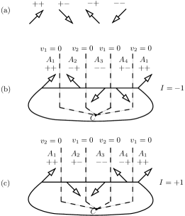
Figure 5: Areas of characteristic behavior and area sequences around a critical point $C$: (a) the four types of characteristic areas $A_{i}$, (b) counterclockwise and (c) clockwise turning behavior of the areas, yielding a critical point of index $-$1 and $+$1, respectively.

Definition 4.4.

Let $\vec{x_{0}}$ be an isolated first-order critical point of $\vec{f}$ defined like above with an area sequence
$(A_{1},\dots,A_{4})$. Then for a pair $A_{i},A_{i+1}$ of adjacent characteristic areas of the area sequence of $\vec{x_{0}}$ (see Fig. 5(a)), a turning in the characteristic behavior of the vector field can be defined. This turning can either be a clockwise turning or a counterclockwise turning as defined in Figs. 5(b) and 5(c), respectively. Since Figs. 5(b) and 5(c) contain all 8 possible configurations of pairs of characteristic areas, only a clockwise or counterclockwise turning behavior can occur and the list in Figs. 5(b) and 5(c) is complete.

Remark 4.5.

One adjacent pair of characteristic areas already determines the whole area sequence in terms of its turning behavior. This is the case because the vector field components whose signs flip are alternating in the area sequence. Thus, an area sequence can either show a clockwise turning behavior or a counterclockwise turning behavior, but not a mixture of these and we will also speak of a clockwise or counterclockwise turning behavior of the area sequence as a whole—a clockwise or counterclockwise area sequence for short.

We can use the turning behavior of area sequences around a critical point to determine its Poincaré index:

Theorem 4.6.

Let $\vec{f}\in C^{1}(E)$ be a vector field like in 4.1 and let $\vec{x_{0}}\in E$ be an isolated critical point of $\vec{f}$ of first order, such that $D\vec{f}(\vec{x_{0}})$ has full rank. If the area sequence of $\vec{x_{0}}$ is counterclockwise, then the Poincaré index of $\vec{x_{0}}$ is $I_{\vec{f}}(\vec{x_{0}})=-1$ and $\vec{x_{0}}$ is a topological saddle of $\vec{f}$. If the area sequence of $\vec{x_{0}}$ is clockwise, then $I_{\vec{f}}(\vec{x_{0}})=+1$ and $\vec{x_{0}}$ is a non-saddle first-order critical point of $\vec{f}$.

Proof.

The area sequence can also be interpreted as a sequence of four qualitative samples of the vector field values lying on a piecewise linear closed curve $\Gamma\subset B_{\epsilon}(\vec{x_{0}})$ that contains $\vec{x_{0}}$ (qualitative in the sense that just the signs of the vector field components are sampled). We will now prove that summing up the angle change of the vector field between these discrete samples and performing this for all four samples yields the same result as evaluating the continuous integral of the change of angle of $\vec{f}$ over a continuous Jordan curve $\hat{\Gamma}$ around $\vec{x_{0}}$, only containing one critical point $\vec{x_{0}}$. Therefore, the Poincaré index of $\vec{x_{0}}$ can be computed by just identifying the sequence of characteristic areas around $\vec{x_{0}}$.

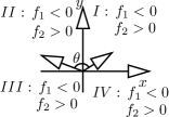
Figure 6: The change of angle of the vector field for two adjacent areas; since only one component flips sign, the two vectors lie in adjacent quadrants I–IV and one has $|\theta|<\pi$.

Let $\tilde{\vec{f}}$ be the linearized system of $\vec{f}$ defined on an $\epsilon$-ball around $\vec{x_{0}}$. Since for two adjacent areas only the sign of one component of $\vec{f}$ changes, the vector at the first sampling point and the vector at the second sampling point lie in two different but adjacent quadrants around $\vec{x_{0}}$ (see Fig. 6). As the value of the linear approximation $\tilde{\vec{f}}$ changes linearly on $\Gamma$ between two sample points and $\tilde{\vec{f}}$ is continuous, the turning behavior is uniquely determined by the two sample points; and since the two sample points lie in adjacent quadrants defined by the coordinate axes, the vector rotates about an angle $\theta$ with $|\theta|<\pi$ when walking on $\Gamma$ from one sample point to the next. Thus, the whole area sequence (for four pairs of areas) yields the total change in angle $\Theta$, with $|\Theta|<4\pi$. As the area sequence wraps around the critical point, the first and the last vector of our sample sequence are the same and thus the change in angle of the vector field has to be $2k\pi$ with $k\in\mathbb{Z}$, see Fig. 5(b) and Fig. 5(c). As $\det D\vec{f}(\vec{x_{0}})\neq 0$, for some $\epsilon$ also $\det D\vec{f}(\vec{x})\neq 0$ for $\vec{x}\in B_{\epsilon}(\vec{x_{0}})$, i.e. the vector field is not constant in a neighborhood of $\vec{x_{0}}$ and one has $k\neq 0$. It is $|k|<2$ because $|\Theta|<4\pi$. Thus, only $k=\pm 1$ is possible and the critical point of the linearized field $\tilde{\vec{f}}$ is of Poincaré index $I_{\tilde{\vec{f}}}(\vec{x_{0}})=\pm 1$.

Since for linear systems all critical points of index $\pm 1$ have been classified (see Sections 3.2 and 3.3 as well as Fig. 2), a critical point can either be a saddle (for $I_{\tilde{\vec{f}}}(\vec{x_{0}})=-1$), if the area sequence shows a counterclockwise turning behavior, or a non-saddle (i.e. a source or sink for $I_{\tilde{\vec{f}}}(\vec{x_{0}})=-1$), if the area sequence shows a clockwise turning behavior. According to the Hartman-Grobman theorem, the Poincaré indices of first-order isolated critical points are invariant under linearization and $\tilde{\vec{f}}$ has a saddle in $\vec{x_{0}}$ if and only if $\vec{f}$ has a topological saddle in $\vec{x_{0}}$, which completes the proof of the theorem. $\square$

4.4 Invariant Operations on the Area Sequence

There are 8 possible area sequences as there are four different areas and each area sequence can be clockwise or counterclockwise. Since these sequences yield only two types of critical points distinguishable by their Poincaré index, it is desirable to build equivalence classes of area sequences that yield critical points of the same Poincaré index. These equivalence classes can be directly constructed using elementary group theory. We refer to the book [Hup67] for a comprehensive overview of the theory of finite groups.

First it is obvious but nonetheless interesting to observe that the turning behavior of the area sequence is invariant under rotation and also invariant under a simultaneous sign flip of both vector field components. Figure 5 illustrates this: for example, the first and the last area pair of Fig. 5(b) and Fig. 5(c) can be related through a sign flip, likewise the second and third area pair.

Rotations and sign flips can be modeled as group operations. Given a group $G$ and a set $X$, a (left) group action of $G$ on $X$ is a mapping $\circ:G\times X\rightarrow X$ denoted $(g,x)\mapsto g\cdot x$ such that $e\cdot x=x$ for all $x\in X$ (here $e$ denotes the neutral element in $G$) and $(gh)\cdot x=g\cdot(h\cdot x)$ for all $g,h\in G$ and all $x\in X$. The orbit of an element $x\in X$ under a group action of $G$ on $X$ is the set $O(x)=\{g\cdot x:g\in G\}$. Orbits of a group action on a set $X$ define equivalence classes on $X$, and the set of all orbits is a partition of $X$.

The rotation of the area sequence is identical to the operation of the cyclic group $C_{4}$ on the indices of the area sequence. The sign flip can be modeled as the operation of a group isomorphic to the symmetric group $S_{2}$ on the signs of the components. From now on, the first group is referred to as the shape group $G_{s}$ and the second group as the (sign) flip group $G_{f}$. The direct product of $G_{s}$ and $G_{f}$ is called the coloring group $G_{c}=G_{s}\times G_{f}$.

Now we define the group action of $G_{c}$ on the set of area sequences. Let $\pi_{r}:G_{c}\rightarrow G_{s}$ be the projection of $G_{c}$ onto $G_{s}$ and $\pi_{f}:G_{c}\rightarrow G_{f}$ the projection of $G_{c}$ onto $G_{f}$. Further, let $g\in G_{c}$ be an element of the coloring group $G_{c}$ with its projections $\pi_{r}(g)=s\in G_{s}$ and $\pi_{f}(g)=f\in G_{f}$ onto the shape group and the flip group, respectively. Then, $g$ acts on an area sequence $(A_{1},\dots,A_{4})$ as defined below:

$$g(A_{1},\dots,A_{4}):=(fA_{s(1)},\dots,fA_{s(4)}),$$

where $s$ is a permutation of the indices $\{1,\dots,4\}$ and $f$ a self-inverse permutation on the set of areas, $\{1,\dots,4\}$. $f$ can be interpreted as an element that flips the signs of all components of the vector field: areas of type $(+,+)=\text{1}$ are mapped to areas of type $(-,-)=\text{4}$ and vice versa; an area of type 2 is interchanged with an area of type 3.

The orbits of this group action on the set of all possible area sequences yield equivalence classes of area sequences such that each equivalence class contains all area sequences that can be mapped onto each other by rotations and sign flips.

4.5 Interpolated Vector Fields

Typical vector field data is given on a grid. Therefore, the vector field needs to be interpolated to obtain values at non-grid points. Local (i.e. cell-wise) interpolation schemes are often chosen for the sake of simplicity and speed. In the following two sections, we will have a closer look at two interpolation schemes: barycentric interpolation on triangles and bilinear interpolation on rectangles.

Both interpolation schemes share some important properties. On the one hand, inside cells, both interpolation schemes are of class $C^{\infty}$ and thus linearizable. On the other hand, they are defined locally or in a piecewise way: a different interpolant is used for each cell. The interpolation is only of class $C^{0}$ across cell boundaries and it is linear and continuous along cell boundaries. Basic concepts and tools are developed for the simpler case of the barycentric interpolant. Then, these tools are adapted and extended for bilinear interpolation.

Note that the case of linear interpolation on triangular meshes can equally efficiently be solved by calculating the rotation along each triangle directly. As there can either be no or exactly one critical point of Poincaré index $\pm 1$ inside each cell, a cell with zero rotation has no critical point on its inside, whereas a nonzero rotation implies that there is a critical point inside the cell and already determines its Poincaré index. None the less we will describe the barycentric setting in the following as the notions introduced there will also be used in the more subtle case of the bilinear interpolant.

5 Barycentric Case

A $d$-simplex $s$ on $d+1$ vertices offers a natural way for the linear interpolation via barycentric coordinates. For the following, we will again restrict the dimension to $d=2$, where a simplex is identical with a triangle.

5.1 Cells

From now, a cell $T$ denotes a triangle with vertices $\vec{x}_{1}$, $\vec{x}_{2}$, $\vec{x}_{3}\in\mathbb{R}^{2}$ and with one real 2D vector (from the vector field) attached to each vertex such that a cell becomes a 3-tuple $T=((\vec{x}_{1},\vec{v}_{1}),(\vec{x}_{2},\vec{v}_{2}),(\vec{x}_{3},\vec{v}_{3}))\subset(\mathbb{R}^{2}\times\mathbb{R}^{2})^{3}$. Most of the time, we are only interested in the vector field values and not the position of the vertices, just writing $T=(\vec{v}_{1},\vec{v}_{2},\vec{v}_{3})$. The vector field inside a cell $T$ will be written $\vec{f}:|T|\rightarrow\mathbb{R}^{2}$, when $|T|\subset\mathbb{R}^{2}$ is the set of convex combinations of the vectors $\vec{x}_{1},\vec{x}_{2},\vec{x}_{3}$. Further, let $\vec{f}=(f_{1},f_{2})^{T}$. We restrict the vector field values on the vertices to be non-zero such that the interpolated vector field has isolated singularities only.

5.2 Sector Sequences and level sets of the Interpolant

The vector field is interpolated component-wise inside the cell using barycentric coordinates. The interpolation is linear, and the interpolant is continuous in the cell and on its boundaries.

Definition 5.1.

Given the cell $T$, let us look only at one component of $\vec{f}$, say $f_{1}$ ($f_{2}$). If two adjacent vertices (i.e. two endpoints of an edge of the cell) have values of $f_{1}$ ($f_{2}$) such that one value is smaller than $\omega$ and the other one bigger than $\omega$, then by virtue of continuity and linearity of the interpolant on cell edges there exists exactly one point on the edge with an $f_{1}$-value ($f_{2}$-value) of $\omega$. Such an edge is called an $\omega$-active edge for $f_{1}$ ($f_{2}$). If the two values are both smaller or bigger than $\omega$, there exists no such point and the edge is called an $\omega$-inactive edge for $f_{1}$ ($f_{2}$).

Remark 5.2.

We can now observe the following:

1) For one cell, there exist at most two $\omega$-active edges for each component and, thus, at most two points on the cell boundary with value $\omega$ for each component if all vertex values of each component differ from $\omega$.

2) Since a critical point of the interpolated vector field can only occur in a crossing point of the 0-level sets of the components of the vector field, a cell with an interior critical point requires two active edges per component. Furthermore, there can at most be one critical point inside a cell because the 0-level sets of the interpolant are straight lines.

3) Since there can only be one critical point inside a cell, the sector sequence around a critical point can be found by looking for intersections of the 0-level sets of the components with the cell boundary. Each active edge yields exactly one 0-value point on a boundary edge, the position of which can be obtained through linear interpolation between adjacent vertices.

If one collects the sequence of 0-value points of the components while traversing the boundary of the cell (as shown in Fig. 7), one can not only construct the area sequence but also determine whether the 0-level sets cross and thus whether there is a critical point of the interpolated vector field. Let $a$ denote a 0-value point of the first component and let $b$ denote a 0-value point of the second component of the vector field. Then, for the sequences $aabb$, $bbaa$, $abba$, or $baab$, the cell does not contain a critical point, whereas for the sequences $abab$ and $baba$, there is a critical point. These $\binom{4}{2}=6$ intersection sequences are all possible sequences for the barycentric interpolant because there can be at most two 0-value points for each component on the boundary of the cell.

The sequence of the crossings of the 0-level sets of the components together with the information of how the signs of the components change defines the sequence of characteristic areas around a critical point and thus its Poincaré index as we have shown in Section 4.3. We will make use of this in the following section.

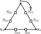
Figure 7: Triangle cell data structure with two edge slots on each edge. An edge slot is identified with a possible 0-value point of one of the vector field components. $S_{ij}$ refers to the $j$-th slot of edge $i$.

5.3 An Edge-Coloring Problem

Before we can classify critical points, a suitable data structure for describing the area sequence around a critical point is needed. Just looking at the sign configuration of the components in the vertices (which can be seen as a coloring of the vertices) does not allow us to distinguish the types of critical points because the area sequence is not fully determined just by the signs of the components in the vertices (see Fig. 8).

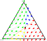
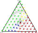
(a)	(b)

Figure 8: Different types of critical points for the same vertex sign configuration: (a) saddle with area sequence $(++,+-,--,-+)$, (b) attracting node with area sequence $(++,-+,--,+-)$.

We use an edge-based data structure to uniquely describe the sequence of 0-values of the vector field components on the boundary of the cell and the area sequence: each cell edge is given two slots that can be filled with 0-value points of the components (see Fig. 7). The slots represent the order of the two components’ zero values while walking around the boundary of a cell. The slots also indicate whether a component changes from positive to negative or from negative to positive values as it passes through a 0-value point. There is no more than one 0-value for each component along a boundary edge of a cell because of the linearity of the interpolation along cell edges. Hence each edge can be given two slots and 13 types of boundary edges can occur, as listed in Table 1. The notation $(f_{1}:+\rightarrow-,f_{2}:-\rightarrow+)$ denotes that $f_{1}$ changes from a positive value to a negative value, $f_{2}$ changes from a negative value to a positive value, and the sign change of $f_{1}$ occurs before the sign change of $f_{2}$ as one traverses the edge on the cell boundary in clockwise direction. If a component is not listed, it indicates that this component has no sign change on that edge and thus no 0-value.

Table 1: The thirteen edge colorings.

Edge type	0-values of components
$\xi_{1}$	no 0-value, neither for $f_{1}$ nor for $f_{2}$
$\xi_{2}$	$(f_{1}:+\rightarrow-)$
$\xi_{3}$	$(f_{1}:-\rightarrow+)$
$\xi_{4}$	$(f_{2}:+\rightarrow-)$
$\xi_{5}$	$(f_{2}:-\rightarrow+)$
$\xi_{6}$	$(f_{1}:+\rightarrow-,f_{2}:+\rightarrow-)$
$\xi_{7}$	$(f_{1}:+\rightarrow-,f_{2}:-\rightarrow+)$
$\xi_{8}$	$(f_{1}:-\rightarrow+,f_{2}:+\rightarrow-)$
$\xi_{9}$	$(f_{1}:-\rightarrow+,f_{2}:-\rightarrow+)$
$\xi_{10}$	$(f_{2}:+\rightarrow-,f_{1}:+\rightarrow-)$
$\xi_{11}$	$(f_{2}:+\rightarrow-,f_{1}:-\rightarrow+)$
$\xi_{12}$	$(f_{2}:-\rightarrow+,f_{1}:+\rightarrow-)$
$\xi_{13}$	$(f_{2}:-\rightarrow+,f_{1}:-\rightarrow+)$

For a triangle cell, each of the three edges can now be of types $\xi_{1}$–$\xi_{13}$, which represent a coloring of the triangle edges with 13 colors. Therefore, such an edge-coloring can be seen as an ordered 3-tuple over the set of the 13 colors. Note that not every possible 3-tuple over the set of colors is a valid coloring as there exist the following types of invalid colorings, i.e. colorings that are not (or not uniquely) mappable to a sign configuration of the vector field at the cell vertices:

1) Colorings that have an invalid number of active edges: For each component, the cell has to have at least two active edges and the number of active edges has to be even.
Example: the coloring $(\xi_{2},\xi_{4},\xi_{1})$ would have one active edge for both $f_{1}$ and $f_{2}$ and would thus be an invalid coloring.

2) Colorings that are not mappable to a sign configuration of the vector field in the cell vertices at all.
Example: a component, say $f_{1}$, cannot change from $+$ to $-$ twice in a row. Thus, for example, a coloring $(\xi_{2},\xi_{2},\xi_{2})$ would be invalid.

Each valid coloring of a triangle can by construction be uniquely mapped to a sign configuration of the values of the vector field components on the vertices (see Fig. 11). However, the edge-coloring of a triangle carries more information than just the sign configuration of the vector field components on the vertices (namely a unique description of the intersection topology of the 0-level sets with the cell boundaries) such that several colorings of the triangle may be mapped to the same sign configuration.

5.4 Classification

As discussed in Section 4.4, there are certain operations that leave the clockwise and counterclockwise turning behavior of the area sequence invariant. These operations can be modeled as a group action of a certain group on the set of area sequences.

Since there exists a bijective map from the set of edge-colorings of a cell $T$ to the set of area sequences (each coloring describes exactly one area sequence), one can make use of the ideas presented in Section 4.4 to construct equivalence classes of cell colorings yielding the same area sequence. Then, all possible edge colorings of a cell can be constructed and classified by using a group action that builds equivalence classes of equivalent colorings. Colorings related by rotation or color flip thus yield the same type of critical point.

Theorem 5.3.

Every configuration of a cell $T$ (as a coloring of the cell) that results in an intersection of the level sets of the two components inside of $T$ and thus contains a critical point is topologically equivalent to one of 8 representative configurations of which four contain a saddle first-order critical point (Poincaré index $-1$) and four contain a non-saddle first-order critical point (Poincaré index $+1$). Representatives for the 8 orbits are listed in Table 2 and visualized (Online Resource 1). Colorings that are not included in this list do not contain a critical point.

Table 2: Representatives of the 8 equivalence classes of colorings of a triangle cell.

Class	Cell coloring	Index
1	$(1,6,9)$	$-1$
2	$(1,7,8)$	$+1$
3	$(1,10,13)$	$+1$
4	$(1,11,12)$	$-1$
5	$(2,4,9)$	$-1$
6	$(2,5,8)$	$+1$
7	$(2,11,5)$	$-1$
8	$(2,13,4)$	$+1$

Proof.

This theorem is proven using a GAP program, see (Online Resource 3).

The basic idea is as follows. Using a combinatoric description, all possible colorings of a cell are constructed: the set of all ordered 3-tuples over the set of all possible colors. Then, a group action on that set is considered to build equivalence classes of colorings such that all pairs of elements of an equivalence class can be mapped onto each other by means of operations leaving the type of critical point invariant, as described in Section 4.4.

Let $\mathcal{C}=\{\xi_{1},\dots,\xi_{13}\}$ be the set of colors as described above and let the set of 3-tuples over $\mathcal{C}$, $\mathcal{T}=\{t=(t_{1},\dots,t_{3}):t_{i}\in\mathcal{C}\}$ be the set of colored cells or tiles. For the coloring group $G_{c}$, which is the direct product of the shape group $G_{s}$ and the flip group $G_{f}$ (see Section 4.4), an action of $G_{c}$ on the set of all colored tiles $\mathcal{T}$ can be defined. Here, the shape group $G_{s}$ is the cyclic group $C_{3}$ as the subgroup of rotations of the symmetry group of the combinatoric triangle (which is given by the symmetric group $S_{3}$). The color flip group is chosen to be $G_{f}=\langle(2,3)(4,5)(6,9)(7,8)(10,13)(11,12)\rangle$, which is isomorphic to $S_{2}$; the numbers in the cycles correspond to the color indices of edge colors. The choice of generator for $G_{f}$ is obvious and unique since simultaneous flipping of signs of the two components results in an interchange of edges with color $\xi_{2}$ and $\xi_{3}$, $\xi_{4}$ and $\xi_{5}$, etc.

Using our GAP program, first all possible colorings of a cell are generated and for each orbit a representative is checked for the validity of the coloring. Elimination of invalidly colored cells can be done on a representative level: if the representative of an orbit is an invalid coloring, all other elements in the orbit are invalid because they are equivalent colorings. Thus, one can talk of invalidly colored orbits.

After discarding all invalidly colored orbits, for the remaining orbits the sequence of 0-value points of the components on the cell boundary is extracted from the coloring. Since the 0-level sets of the components are straight lines, the sequence of 0-value points determine whether the 0-level sets intersect within the cell (thus yielding a critical point) or not (no critical point). If the 0-level sets intersect within the cell, the area sequence and its turning behavior are extracted to classify the type of critical point as saddle (Poincaré index $-$1) or non-saddle (Poincaré index $+$1). As all critical points are of first-order, this classification by the Poincaré index covers all possible types of critical points. Since all possible colorings have been considered the list of equivalence classes is complete. See (Online Resource 1) for a list of all equivalence classes, including sample visualizations. $\square$

6 Bilinear Case

In this section, the concepts developed in the previous section are transferred to the bilinear case. Most elements can be immediately adopted, but some caution has to be taken because the interpolant is no longer linear.

6.1 Interpolation Scheme and Cells

Bilinear interpolation is an extension of linear interpolation for interpolating functions of two variables. This interpolation scheme is simple, fast to implement, and widely used in many visualization algorithms working in a cell-wise fashion on uniform, rectilinear, or curvilinear 2D grids.

A cell $Q$ is represented by an ordered 4-tuple on the points $\vec{x}_{1},\dots,\vec{x}_{4}\in\mathbb{R}^{2}$ with one real-valued 2D vector (the vector field values) attached to each vertex such that a cell becomes a 4-tuple $Q=((\vec{x}_{1},\vec{v}_{1}),\dots,(\vec{x}_{4},\vec{v}_{4}))\subset(\mathbb{R}^{2}\times\mathbb{R}^{2})^{4}$. Mostly, we are only interested in the vector field values, just writing $Q=(\vec{v}_{1},\dots,\vec{v}_{4})$.

Any uniform, rectilinear, or convex curvilinear cell can be transformed to the unit square $[0,1]^{2}$ in terms of a diffeomorphism, yielding local Euclidean coordinates $s,t\in[0,1]$ within the cell. Without loss of generality we therefore only consider the case of Euclidean coordinates in the following, i.e. the setting when the interpolation scheme is employed in parameter space. We use the following notation for bilinear interpolation:

Let $B_{i}:[0,1]\times[0,1]\rightarrow\mathbb{R}$, $i=1,2$, be bilinear functions for the two vector components (corresponding to $x$ and $y$), defined by

$$B_{i}(s,t):=(1-s,s)\begin{bmatrix}{v_{1i}}&{v_{2i}}\\ {v_{3i}}&{v_{4i}}\end{bmatrix}\left(\begin{array}[]{c}1-t\\ t\end{array}\right),$$

where $s,t\in[0,1]\subset\mathbb{R}$ are local coordinates within one cell and $\vec{v}_{1}=({v_{11}},{v_{12}})^{T}$,…,$\vec{v}_{4}=({v_{41}},{v_{42}})^{T}$ are the values of the vector field components at the four vertices $\vec{x}_{1},\dots,\vec{x}_{4}$. Then $\vec{B}=(B_{1},B_{2})^{T}$ is called the bilinear interpolant of $\vec{v}_{1},\dots,\vec{v}_{4}$.

Remark 6.1.

The bilinear functions can be rewritten as

$$B_{i}(s,t)=a_{i}s+b_{i}t+c_{i}st+d_{i},$$ (6.1)

with $a_{i}={(v_{3i}-v_{1i})}$, $b_{i}={(v_{2i}-v_{1i})}$,
$c_{i}={(v_{1i}-v_{2i}-v_{3i}+v_{4i})}$ and $d_{i}=v_{1i}$.

The following properties of the interpolant will be of importance throughout the rest of the section:

1. The $\omega$-level sets of $B_{i}$ are hyperbolas, which can be seen when writing the interpolants in standard form (6.1) and interpreting them as conic sections. Some examples of $\omega$-level sets of $B_{i}$ are depicted in Fig. 9.

2. The interpolation is linear in each dimension and continuous. Furthermore, the interpolation along edges of the cell is linear: analogously to the barycentric case in Section 5, one can define $\omega$-active and $\omega$-inactive cell edges. There exist four points on a cell boundary with value $\omega$ and thus most four $\omega$-active edges, if all vertex values differ from $\omega$.

3. In the case $c_{i}=0$, $B_{i}(s,t)$ is a linear function. If $c_{i}\neq 0$, $B_{i}(s,t)$ is nonlinear and when looking at the partial derivatives $\frac{\partial}{\partial s}B_{i}(s,t)=c_{i}t+a_{i}$ and $\frac{\partial}{\partial t}B_{i}(s,t)=c_{i}s+b_{i}$, one sees that $B_{i}(s,t)$ has an extremal point at $S_{i}(-\frac{b_{i}}{c_{i}}|-\frac{a_{i}}{c_{i}})$. This extremal point is a saddle because the Jacobian $DB_{i}$ is singular at $S_{i}$ and for all $s,t\in\mathbb{R}$ the Hessian $H_{i}$ of $B_{i}$ has a negative determinant (and thus its eigenvalues are of opposite sign; see Figs. 9 and 12 for examples).

6.2 Bilinear Interpolation of Scalar Fields

Let us look at the qualitative behavior of a bilinearly interpolated scalar fields before extending this to vector fields. We only consider one $B_{i}$ here, say $B_{1}$, as a placeholder for a scalar field. The qualitative behavior of the interpolant within the cell can be described in terms of its vertex configuration:

Theorem 6.2.

Given $\omega\in\mathbb{R}$ and a cell $Q$ with vertex values $v_{11}$, $v_{21}$, $v_{31}$ and $v_{41}$, $v_{i1}\neq\omega$ for $1\leq i\leq 4$, four cases for the qualitative behavior of $\omega$-level sets of the interpolant $B_{1}(s,t)$ within a cell can occur: Fig. 9 summarizes these cases that depend on the classification of vertex values $v_{i1}$ being greater or less than $\omega$. Here, active and inactive edges for a cell $Q$ are defined in the same way as for the barycentric interpolant in Definition 5.1. Please note that we use the terminology saddle cell (see Fig. 9) to describe a configuration of vertex values $v_{i1}$, which is different from the classification of a critical point as a saddle point. In the following, we denote the first always by the compound term saddle cell.

All of the statements follow immediately from the continuity of the interpolant and its linearity along cell boundaries.

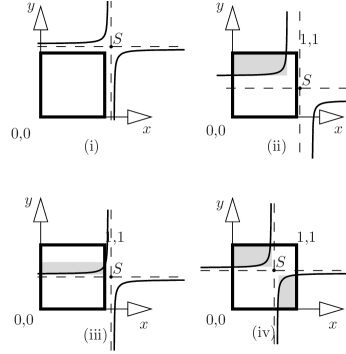
Figure 9: Examples of the four qualitatively distinct configurations of 0-level sets of bilinearly interpolated scalar fields: (i) inactive cell, (ii) single active cell, (iii) couple active cell, (iv) saddle cell. Bounding boxes (see Lemma 6.4) are shown in gray.

Remark 6.3.

For an easier notation of the different cell types in terms of the definitions of Theorem 6.2, we write a cell $Q=(\vec{v}_{1},\vec{v}_{2},\vec{v}_{3},\vec{v}_{4})$ as a 4-tuple over the set $\{+,-\}$ where the $i$-th entry of that tuple is set to $+$ if $\vec{v}_{i}>\omega$ and to $-$ otherwise. Table 3 summarizes this tuple notation, referred to as vertex sign configuration, as in the barycentric case.

Table 3: Different cell types by vertex sign configuration.

Cell type	Vertex sign configuration
inactive	$(-,-,-,-),(+,+,+,+)$
single active	$(-,-,-,+),(+,-,-,-),(+,+,+,-),$
	$(-,+,-,-),(-,-,+,-),(-,+,+,+),$
	$(+,-,+,+),(+,+,-,+)$
double active	$(-,-,+,+),(+,-,-,+),(+,+,-,-),$
	$(-,+,+,-)$
saddle cell	$(-,+,-,+),(+,-,+,-)$

Lemma 6.4 (Bounding-box lemma).

Let $B_{i}(s,t)$ be a bilinear interpolant on a rectangular grid cell $Q$ and let the cell be $0$-active. For each curve of the $0$-level set connecting two $0$-value points $A(A_{x}|A_{y})$, $B(B_{x}|B_{y})$ on the boundary of the cell, the Cartesian product

$$\begin{array}[]{@{}lll@{}}L&=&[\min\{A_{x},B_{x}\},\max\{A_{x},B_{x}\}]\\ &&\times[\min\{A_{y},B_{y}\},\max\{A_{y},B_{y}\}]\end{array}$$

defines a bounding box: the curve of the $0$-level set of $B_{i}$ is inside $L$ except at the $0$-value points at the border of the cell. See Fig. 9 for an illustration of the set $L$ for some sample configurations.

Proof.

We only give a sketch of the proof. The basic idea is the following.

Let the bounding box $L$ be given as the convex hull of the four points

$$\begin{array}[]{l}P_{1}(\min\{A_{x},B_{x}\}|\min\{A_{y},B_{y}\}),\\ P_{2}(\min\{A_{x},B_{x}\}|\max\{A_{y},B_{y}\}),\\ P_{3}(\max\{A_{x},B_{x}\}|\max\{A_{y},B_{y}\}),\\ P_{4}(\max\{A_{x},B_{x}\}|\min\{A_{y},B_{y}\}).\end{array}$$

Note that $A,B\in L$. Then, the bilinear interpolant $B_{i}(s,t)$ restricted to the bounding box $L$ can be expressed in terms of another bilinear interpolant $\hat{B}_{i}(\hat{s},\hat{t})$ defined on $L$ and interpolating the values of the points $P_{1},\dots,P_{4}$. To leave $L$, a 0-isoline of $\hat{B}_{i}$ has to cross the boundary of $L$. Thus, a crossing 0-isoline can only occur where the value of $\hat{B}_{i}$ on the boundary of $L$ is 0. One can then show that apart from the two 0-values in the corner points $A$ and $B$ of a $L$, there exist no other boundary points of $L$ with 0-value. Therefore, such a crossing cannot occur and the 0-level set of $\hat{B}_{i}$ completely lies inside $L$ and cannot leave $L$.

Since the interpolation function $\hat{B}_{i}$ along the boundary of $L$ is continuous and linear, it is sufficient to show that only two points in the set $L$ have 0-value. It then follows immediately that these are the only points on the boundary with zero value. This can be shown easily for a representative of each of the cases listed in Theorem 6.2 and Fig. 9. $\square$

6.3 Analytical Computation of the Position of Critical Points

The position of critical points of the bilinear interpolant $\vec{B}=(B_{1},B_{2})$ can be computed as intersection points of 0-level sets of $B_{1}$ and $B_{2}$ by solving

$$\vec{B}(s,t)=\left(\begin{array}[]{c}B_{1}(s,t)\\ B_{2}(s,t)\end{array}\right)=\left(\begin{array}[]{c}a_{1}s+b_{1}t+c_{1}st+d_{1}\\ a_{2}s+b_{2}t+c_{2}st+d_{2}\end{array}\right)=\vec{0}.$$ (6.2)

Since both $B_{1}(s,t)=0$ and $B_{2}(s,t)=0$ are linear or quadratic equations in $s,t$, the system can either be combined into a single linear or quadratic equation in $s$ or $t$. We will refer to this equation as the intersection equation. Since the linear case occurring here can be treated in exactly the same way as the barycentric case described in Section 5, this degenerate case will be excluded in the following and we will only speak of the (quadratic) intersection equation with discriminant $\Delta$. The equation can either have no real solution ($\Delta<0$), two different real solutions ($\Delta>0$), or a double real solution ($\Delta=0$), and the number of solutions of the intersection equation gives the number of critical points, see Fig. 10.

Since the sign of the discriminant $\Delta$ determines whether the vector field has no, one, or two critical points, it can be interpreted as a bifurcation parameter of a dynamical system, where $\Delta=0$ is the bifurcation value. Also $\Delta$ can be interpreted as a measure for the stability of the critical point—critical points with $\Delta=0$ are generally not stable, whereas the case with two ($\Delta>0$) or no intersection points ($\Delta<0$) can be more or less stable according to the magnitude of $|\Delta|$.

Given a rectangular cell with the vector field values
$\vec{v}_{1},\dots,\vec{v}_{4}$ one can write the components of the bilinear interpolant in normal form like done in (6.2) (see Remark 6.1).

The intersection points of the 0-level sets of the components are obtained by solving (6.2). First, we determine which of the interpolants is linear in $s$ and $t$ (i.e. for which $c_{i}=0$); if both are linear, (6.2) becomes a linear system and can be solved separately yielding one or no solution (and not infinitely many solutions as the singularities are restricted to be isolated). If one of the interpolants is linear and the other nonlinear, the linear one can be solved for $s$ or $t$ and this can be plugged into the other to yield a quadratic equation in $s$ or $t$. If both interpolants are nonlinear, one can be solved for $s$ or $t$ and plugged into the other.

All these equations have at most two real solutions yielding one coordinate of the 0-value points of the interpolated vector field. The other coordinate can be obtained through the linear or quadratic equation between $s$ and $t$ from the first step. A solution within the cell is found by restricting the coordinates to be in $[0,1]^{2}$. Note that the vector field values for each component are always restricted to be nonzero at cell vertices and that the two components are assumed not to be exactly the same.

6.4 Level Sets and Sector Sequences

Each solution of (6.2) lies in the intersection set of the 0-level sets of $B_{1}$ and $B_{2}$. The following cases can occur when looking at the intersections of level sets of $B_{1}$ and $B_{2}$:

Theorem 6.5.

Let $c_{1}$, $c_{2}$ be the 0-level sets of $B_{1}$, $B_{2}$ and let $\Delta\in\mathbb{R}$ be the discriminant of the intersection equation for a cell $Q$. Then, the following cases can occur:

1. $\Delta<0$ $\leavevmode\nobreak\ \Leftrightarrow\leavevmode\nobreak\$ $c_{1}$, $c_{2}$ are disjoint and there is no critical point (see Fig. 10(a)),

2. $\Delta=0$ $\leavevmode\nobreak\ \Leftrightarrow\leavevmode\nobreak\$ $c_{1}$, $c_{2}$ touch in one point (see Fig. 10(b)),

3. $\Delta>0$ $\leavevmode\nobreak\ \Leftrightarrow\leavevmode\nobreak\$ $c_{1}$, $c_{2}$ intersect in two points (see Fig. 10(c)).

Proof.

Clearly one has: $c_{1}$ and $c_{2}$ are disjoint $\leavevmode\nobreak\ \Leftrightarrow\leavevmode\nobreak\$ $\Delta<0$ which proves 1). The same holds for 2). Now it remains to show 2), i.e. that $c_{1}$ and $c_{2}$ cannot touch twice and that the intersection equation has a double solution iff $c_{1}$ and $c_{2}$ touch in one point.

Suppose that $c_{1}$ and $c_{2}$ touch in one point as shown in Fig. 10(b). A small perturbation of the vector field values now either results in a case where the hyperbola branches do not intersect (i.e. $\Delta<0$) as shown in Fig. 10(a), or it yields a case where $c_{1}$ and $c_{2}$ intersect in two points, i.e. where the intersection equation has two different solutions as shown in Fig. 10(c). As each pair of branches can be perturbed separately a double touching case cannot exist as this could be perturbed to yield a triple intersection of the branches which is a contradiction to the maximum number of real solutions of the intersection equation. This proves 3). $\square$

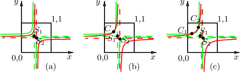
Figure 10: Intersection cases for the 0-level sets (red and green lines) of the two vector field components: (a) no intersection with $\Delta<0$, (b) one touching point $C$ with $\Delta=0$, and (c) two intersection points $C_{1}$ and $C_{2}$ with $\Delta>0$. The saddle points $S_{i}$ $(i=1,2)$ of the two interpolants $B_{i}$ and their asymptotes (dashed lines) are depicted in red for $B_{1}$ and green for $B_{2}$.

6.5 Critical Points and Area Sequences

Let us now look at the types of critical points yielded for the different intersection cases for the 0-level sets of the components as investigated in Theorem 6.5.

1) The case $\Delta<0$, where the 0-level sets do not intersect, is trivial.

2) For the case $\Delta>0$, when the 0-level sets of the components intersect twice, yielding two first-order isolated critical points of the interpolated vector field of first order as none of the directional derivatives is $\vec{0}$ in the intersection points. For each critical point separately, the same things hold as for critical points in the barycentric case; in particular we can look at area sequences, turning behavior of those, etc. for each critical point separately.

Remark 6.6.

The area sequences of the two critical points always share three characteristic areas and these are traversed in opposite directions for each of the points (i.e. clockwise turning for an area pair becomes a counterclockwise turning and vice versa). Therefore, one of the two points has a Poincaré index of $-1$ and the other one has a Poincaré index of $+1$. Another way to see this is the fact that to first observe that there are at most two critical points inside a cell and that the Poincaré index of a cell can either be $-1$, $0$ or $+1$. Now, by virtue of the summation theorem for the Poincaré index, two critical points inside a cell of the same index would force the cell to have an index of $\pm 2$, a contradiction.

3) For the touching case ($\Delta=0$) of the 0-level sets, the tools developed in the previous sections cannot be applied: when linearizing the field around the touching point, the 0-level sets of the two components are tangential to each other and the Jacobian has at least one zero eigenvalue. Thus, the critical point is not of first-order and a well-defined area sequence does not exist for this case. However, a perturbation of the field yields two critical points, one of index $+1$ and one of index $-1$. Then, Poincaré index theory states that the one critical point yielded by the touching of the 0-level sets has an index equal to the sum of the indices of the two critical points it splits into, i.e. the second-order critical point from a touching of the 0-level sets has index 0.

6.6 Edge Coloring and Invariant Operations on the Colorings

As the bilinear interpolant is linear along the cell edges, one can employ the same ideas as in the barycentric case in order to determine existence and types of critical points inside a cell, again using an edge-based “slot” data structure. Using a data structure with two slots for each edge of a cell, one can see this as a cell coloring problem with a coloring of a cell represented as a 4-tuple over the set of 13 colors like described in Section 5.3.

Investigating the intersection topology of the 0-level sets becomes more complicated because the 0-level sets are no longer straight lines. Using the same notation as for the barycentric case, a sequence of 0-value points $aabb$ (where again $a$ stands for a 0-value point of the first component of the vector field and $b$ for a 0-value of the second component) not necessarily has no intersections. Here, it can either yield a case where the isolines have no point in common, touch in one point, or intersect twice as shown in Fig. 1.

The question is whether for a sequence of 0-value points of the form $\dots aa\dots$ or $\dots bb\dots$ the subsequence $aa$ or $bb$ can yield a touching or intersection of the 0-level sets or not. If not, the part $aa$ or $bb$ of the sequence is irrelevant for the intersection topology and can be ”collapsed”, e.g. a sequence $baababab$ for which $aa$ cannot yield a touching of the isolines could be reduced to $bbabab$. If now $bb$ would yield no intersection we could reduce once more to yield $abab$, a sequence which cannot be collapsed any more.

For a fully reduced sequence, we can either determine the number of crossings and thus critical points inside the cell as done in the barycentric case (for sequences of the form $(ab)^{n}$, $n\in\mathbb{N}_{0}$) or we know that the case is value-dependent, i.e. the number of intersections of the isolines cannot be determined just by looking at the topology of the 0-value points on the boundary of the cell. The latter is the case when the fully reduced sequence contains a subsequence $aa$ or $bb$.

The question remains: how can one determine which subsequences of type $aa$ or $bb$ can be collapsed? Let us first focus on non-saddle cells. The bounding box lemma (Lemma 6.4) gives us valuable information for the case of single or double active cells. It states that cases $aabb$ with single active cells for both components lying at opposite vertices of one edge cannot intersect, whereas all other configurations with single and double active cells for the two components—although having no intersection in the topology of 0-value points on the boundary—can be perturbed to yield a touching or an intersection of the isolines and thus are value-dependent.

6.7 Saddle Cells

There are several subtleties that have to be considered when dealing with saddle cells. For one or both components of the vector field, both branches of the 0-level sets intersect with the cell. The topology of the 0-level sets inside the cell is not uniquely determined by the sequence of 0-value points of the components on the cell boundary. This ambiguity can be resolved by adopting the asymptotic decider [NH91].

To determine the intersection topology for the 0-levelsets inside the cell, one can sort the 0-value points by their local coordinates inside the cell in ascending (or descending) order. Then, for each component, the first and second and the third and fourth point in the sorted sequence of 0-value points belong pairwise to the same branch of the 0-level set.

To model this behavior, the previously used edge-based data structure is insufficient because the asymptotes imply a “linking” of two opposite edges of a cell. Therefore, the data structure needs to be extended to describe the position of the 0-value points in the sequence sorted by local coordinates. A natural choice for this is a double-edge data structure shown in Fig. 11(a), which describes a cell by a pair of double edges with four slots for each edge. When filling the slots with 0-value points of the components, their position in the sorted sequence for each coordinate is the index in the respective double edge if one arranges the slots as in Fig. 11(a).

Each valid double-edge configuration can be uniquely mapped to a valid edge coloring configuration via a natural projection $\pi_{1}$ (every valid double-edge configuration can be uniquely mapped to a edge coloring of a cell), which in turn can be mapped to a vertex sign configuration via a natural projection $\pi_{2}$ (every valid edge coloring can be uniquely mapped to a vertex sign configuration of a cell), as described before for the barycentric case. Figure 11 illustrates all three levels of representation.

Using the double-edge data structure, one can now construct all possible double-edge configurations for the case of a saddle cell and check for the intersection topology of the 0-level sets of the interpolant. As we will see in the following, the asymptotic decider plays no role in the types of critical points yielded inside a cell, i.e. there is no need to pay attention to how the 0-value point sequence is reduced when determining the intersection topology and area sequence for saddle cells.

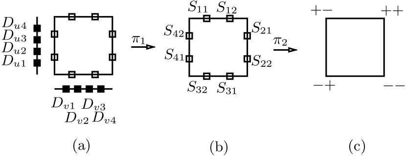
Figure 11: Hierarchy of data structures to describe the sequence of 0-value points on the cell boundary from fine to coarse: (a) double-edge data structure consisting of two double edges with four slots, which can be projected via $\pi_{1}$ to (b) the edge data structure consisting of four edges with two slots each that can finally be projected via $\pi_{2}$ to (c) the vertex sign configuration of the components.

An open question is how the $0$-value sequence can be reduced in a valid way as it was done for non-saddle cells before. The tools provided by the bounding box lemma (Lemma 6.4) and Theorem 6.5 are instrumental here. Figure 12 shows models of the two cases that contain reducible subsequences of type $aa$ or $bb$ in their sequences of 0-value points on the boundary. All other configurations can yield a touching or double intersection of the branches for the same boundary topology and thus are value-dependent (by virtue of Lemma 6.4 and Theorem 6.5).

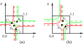
Figure 12: Examples of topologies of 0-value points of the components on the boundaries that can be reduced: (a) $baababba$, which can be reduced by collapsing the branch in the top right which cannot touch or intersect with other branches (bounding box lemma) to $bbabba$, (b) $abababba$, which can be reduced to $abab$ as the two branches in the top left cannot touch or intersect with others (bounding box lemma) or themselves (Theorem 6.5). Again, the saddle points $S_{i}$ $(i=1,2)$ of the two interpolants $B_{i}$ and their asymptotes (dashed lines) are depicted in red for $B_{1}$ and green for $B_{2}$.

Now that we have the tools to construct and reduce 0-value point sequences for cells with bilinear interpolants, let us proceed in the same way as we did for the barycentric case, classifying all cell colorings in terms of the types of critical points they (may) yield inside the cell.

6.8 Classification

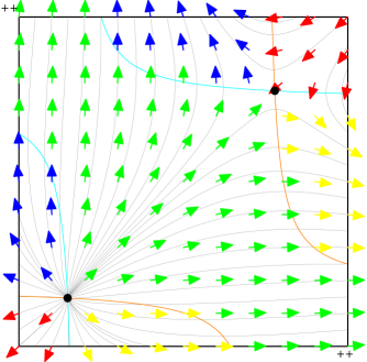
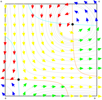
Figure 13: Two example visualizations of vector fields for which the $0$-value sequence on the cell boundary cannot be reduced, yielding two critical points inside the cell.

Theorem 6.7.

Every configuration of a cell $Q$ (as a coloring of the cell) that yields an intersection or touching of the level sets of the two components inside of $Q$ is topologically equivalent to one of 74 representative configurations, see (Online Resource 2) for a complete list:

• 38 configurations have exactly one first-order critical point, the index of which is $\pm 1$ and which is determined by the sequence of characteristic areas on the boundary of the cell.

• 4 configurations have two critical points, one of which is a saddle (i.e. index $-$1) and the other a non-saddle (i.e. index $+$1). Both critical points are stable. See Figure 13 for visualizations of two sample cases.

• 32 configurations are value-dependent, i.e. they have either no, one, or two critical points. The case of a single critical point is an unstable bifurcation point of the underlying dynamical system.

Colorings that are not included in this list cannot have a critical point inside the cell.

Proof.

The proof is analogous to the proof of Theorem 5.3. The corresponding GAP program performs the following steps.

1) Create all possible cell colorings with the 13 colors and use a group action of the coloring group $G_{c}=G_{s}\times G_{f}$ given by the direct product of the shape group $G_{s}$ and the flip group $G_{f}$ on the set of all colored cells to obtain equivalence classes of colored cells (that contain the same number and types of critical points). The flip group only depends on the colors and as these have not changed it can be chosen as in the proof of Theorem 5.3. The shape group $G_{s}$ is chosen as the cyclic group $C_{4}$ of the rotations of a cell by $\frac{\pi}{2}$ as a subgroup of the full symmetry group of the square, which is the dihedral group $D_{8}$ of order $8$.

2) Examine the representatives of the orbits: sort out invalid colorings as in the proof of Theorem 5.3 and determine the intersection topology and the reduced 0-value sequence of the 0-level sets of the two components using the properties described in the preceding sections. This yields an area sequence that can be used to determine the number and types of critical points inside the cell. Here, four classes of configurations are distinguished: cases with exactly one critical point, cases with exactly two critical points, cases that are value-dependent, and cases that yield saddle cells for any component.

3) Determine the turning behavior of the reduced area sequence and thus the type of critical point for configurations with exactly one critical point. Value-dependent and double intersection cases need no further treatment as the number and types of the critical points are not fully determined by the area sequence.

4) For saddle cells: construct all possible double-edge configurations and the reduced 0-value sequence for each configuration yielding an area sequence.

As it turns out, for saddle cells all double-edge configurations yield the same number and the same types of critical points such that the asymptotic decider indeed does not influence the types of critical points inside a cell as claimed in Section 6.7. For the other cases, the number of equivalence classes given in the theorem arise. A full list of cases, including example diagrams, is provided in (Online Resource 2). $\square$

7 Boundary Points and Closed Streamlines

So far the issue of critical points on cell boundaries has not been addressed and is somewhat delicate because the interpolation scheme is only $C^{0}$ across cell boundaries for both the barycentric and the bilinear cases.

To resolve this issue, we employ a cell clustering as described by Tricoche et al. [TSH00]: the current cell with a critical point at the cell boundary and its neighboring cell sharing the edge with the critical point are clustered into a super cell, see Fig. 14. This process is iterated as long as there are critical points on the cell (or super cell) boundary. Then, a new (artificial) critical point $C^{\prime}$ is positioned inside the super cell at a position given by the averaged positions of the critical points inside the super cell. This new critical point $C^{\prime}$ can be of arbitrary order and complexity. In order to determine the topology of the vector field inside the super cell, the super cell is triangulated with a new inner vertex at the position of $C^{\prime}$. Subsequently, a piecewise linear vector field is constructed inside the super cell as the union of the barycentrically interpolated vector fields on the triangles, using the information from the boundary of the super cell. As the direction of the new vector field does not change on rays emerging from $C^{\prime}$, hyperbolic sectors around $C^{\prime}$ can be identified by looking at the configuration of the vector field on the boundary of the super cell. After identification of the boundaries of hyperbolic sectors, the separatrices can be traced beginning from the super cell boundary in the usual way. Figure 15 shows how the different sector types around the critical point $C^{\prime}$ can be determined by using a sequence of orientations of the vector field in relation to the position vector on the boundary of the super cell with respect to the origin $C^{\prime}$. We refer to [TSH00] for details of the method. This is a local method that does not alter the vector field behavior outside the super cell; thus, it is a robust and simple way to deal with critical points on cell boundaries. Note that the data of the randomly generated test vector fields as shown in Table 4 suggest that boundary critical points occur extremely seldom such that the additional steps needed by the algorithm in that case are negligible regarding its speed.

Another problem not addressed so far is the task of finding limit cycles of vector fields. Since this problem has been addressed in various publications already (see [WS01, TWHS04]) and the methods presented there can be incorporated in our algorithm, we will not deal with this case here.

Figure 14: Forming a super cell consisting of the quadrangular cells $Q_{1}$ and $Q_{2}$ for a case where a critical point $C$ lies on the cell boundary of $Q_{1}$ and $Q_{2}$. The super cell is then triangulated by $T_{1},\dots,T_{6}$ and the vector field (shown in gray) is interpolated barycentrically inside each triangle $T_{i}$.

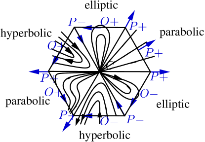
Figure 15: Possible configurations of the orientation of the vector field in relation to the position vector with respect to the origin $C^{\prime}$. $P$ denotes a parallel configuration, $O$ an orthogonal one. The appended signs $+$ and $-$ distinguish the two possible directions of the vector field w.r.t. the position vector in each case.

8 Algorithm

The algorithm consists of three main stages. First, all cells that may contain critical points are identified. Then, these cells are examined more thoroughly to check whether they contain one or more critical points and whether cell clustering is needed. This step is performed by computing the coloring of the cell and using a lookup table to determine the class of the cell coloring as defined in Theorems 5.3 and 6.7. Finally, the positions of the critical points inside the cells are computed analytically. For non-saddles, the type can either be classified using the Jacobian at that point or the sector-based idea described in [TSH00], which is also used to determine the types of higher-order critical points. Note that the exact type of first-order non-saddles is not required to build the topological skeleton, which is only based on trajectories originating from hyperbolic sectors.

8.1 Generic Algorithmic Skeleton

1. Traverse cells, mark cells that have at least two active edges for each component by looking at the sign configuration of the vector field at the vertices.

2. Compute cell colorings of the marked cells and fetch the configuration class for each cell in the lookup table; a perfect hash function can be used for this. Deal with critical points on the boundary of the cell using the cell-clustering approach as described in Section 7.

3. Compute the location(s) of the critical point(s) inside the cell. For the barycentric case, a linear system is solved. For the bilinear case, one can write the interpolant for each component in normal form $B_{i}(s,t)=a_{i}s+b_{i}t+c_{i}st+d_{i}$ and combine the two equations into the linear or quadratic intersection equation in $s$ or $t$. Then the discriminant $\Delta$ of the intersection equation and its solutions are computed. For both cases, solutions lying outside the cell are dropped.

4. Construct the topological skeleton of the vector field in the usual way tracing streamlines at the boundary of hyperbolic sectors and connecting these to other critical points or boundary points when they get close. The boundaries of hyperbolic sectors can either be found as described by Tricoche et al. [TSH00] or by using the eigenvectors of the Jacobian at the critical point. Our implementation employs an adaptive explicit Runge-Kutta method for streamline tracing.

8.2 Performance and Topology Simplification

We propose that, in order to overcome numeric problems in the vicinity of critical points, streamlines are only traced from and to boundaries of cells that contain critical points. Within these cells, streamlines are approximated by a straight line connecting the intersection point of the trajectory and the cell boundary with the critical point. This approach has the advantage that typically many small steps of an explicit solver in the vicinity of the critical point can be saved, thus speeding up the calculation of the topological skeleton.

Further simplifications leading to speed-ups can be considered. First, for small cells, the location of the critical point can be reasonably well approximated by placing the critical point at an arbitrary position—say, the center—of the cell. Second, the topology of the vector field for cells with two critical points can be simplified by replacing the two first-order critical points by a single artificial second-order critical point.
The position of the second-order critical point can be approximated by the midpoint of the straight line connecting the two first-order critical points.

8.3 Numerical Stability

To be numerically stable an algorithm has to yield consistent results for the same input data, no matter how the input data is ordered. This is especially important for floating-point data, where the result of interpolation may depend on the interpolation direction and order of instructions. For the algorithm in Section 8.1, this means that no matter how a cell is oriented in terms of the geometric location of its vertices, the result of the calculations has to be invariant for the two cells. This can be achieved by choosing a unique interpolation direction along cell edges such that this choice always yields the same sequence of calculations on the floating-point vector field data. Then, by virtue of consistency of IEEE floating-point arithmetic [IA85], the interpolation result and the corresponding vertex and edge classifications have to be identical.

Consider a cell with vertices $P_{1},\dots,P_{n}$, $P_{i}(x_{i}|y_{i})$
($i=1\dots n$), where $x_{i}$ and $y_{i}$ are floating-point numbers.
Then, without loss of generality one can choose the interpolation direction along an edge between two vertices to always point from the vertex with smaller $y$-coordinate to the vertex with greater $y$-coordinate. If the two $y$-coordinates agree, then the same argument can be applied to the $x$-coordinates of the vertices. This method always yields a unique interpolation direction as: (1) the inequality comparison operator for IEEE floating-point numbers is consistent in the sense that if $f_{1}$ and $f_{2}$ are two floating-point numbers, $f_{1}>f_{2}\leavevmode\nobreak\ \Rightarrow\leavevmode\nobreak\ f_{2}<f_{1}$; (2) the equality comparison operator for IEEE floating-point numbers is commutative, i.e.
$f_{1}=f_{2}\leavevmode\nobreak\ \Rightarrow\leavevmode\nobreak\ f_{2}=f_{1}$.

Our algorithm and the classification of the critical points depend on a consistent orientation of traversing the boundary of a cell. This orientation can be defined by the sign of the oriented area of a cell. For a triangle with vertices $P_{1}(x_{1}|y_{1})$, $P_{2}(x_{2}|y_{2})$, $P_{3}(x_{3}|y_{3})$, the oriented area is

$$A^{*}=\frac{1}{2}(x_{2}-x_{1})(y_{3}-y_{1})-(y_{2}-y_{1})(x_{3}-x_{1}).$$

For the case of quadrilateral cells, a cell is split into two triangles and the oriented area sequence of one of the two triangles can be used.

9 Results

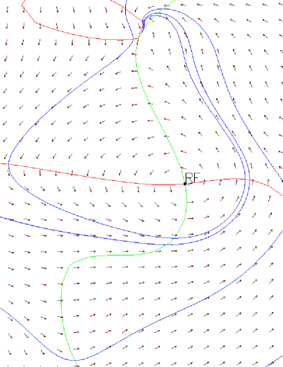
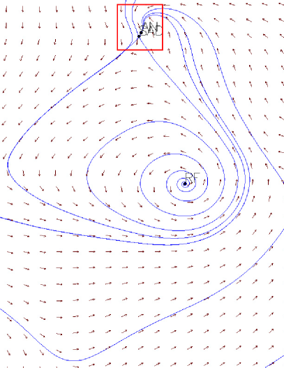
(a) (b)

Figure 16: Vector field topology of the oceanic flow data set. Black dots indicate detected critical points, blue lines show the topological skeleton, annotations provide the classification (AN: attracting node, RF: repelling focus, SAD: saddle). (a) Incorrect topology obtained by a method that intersects linearized 0-level sets of the $x$-component (red) and the $y$-component (green). Notice how trajectories terminate in critical points that are not detected as such in the top left of the image. (b) Correct topology obtained with our method. The pair of critical points inside a value-dependent cell is correctly identified (framed area shown magnified in the bottom right).

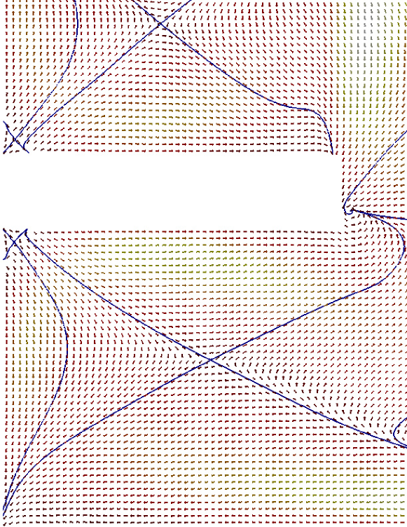
Figure 17: Vector field topology of the air flow data set calculated with our algorithm. Separatrices are shown in blue along with a glyph-based visualization of the vector field, where the arrows encode the vector direction and the vector norm is color-coded.

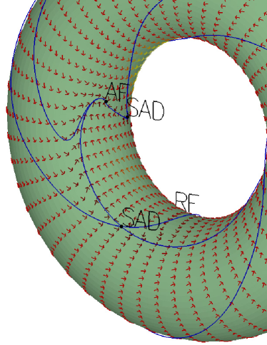
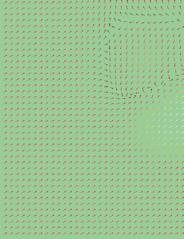
Figure 18: Example of a vector field on a torus. Left: torus immersed in Euclidean 3-space, right: torus in parameter space. The top and the bottom as well as the left and the right border are identified, respectively. Again, the vector field is also visualized via glyphs.

We illustrate the results of our algorithm for four test cases. The first test case consists of randomly generated bilinearly interpolated vector fields: for each cell vertex, the two vector field components are random numbers lying in $[\text{-1,1}]\backslash\{\text{0}\}$, quantized to $\text{10}^{\text{-6}}$. Machine accuracy is set to $\epsilon=\text{10}^{\text{-9}}$ and the threshold of a critical point being of second-order is chosen to be $\Delta<\text{0.05}$, where $\Delta$ is the discriminant of the intersection equation as described in Section 6.3. We have generated and examined $10^{8}$ cases. The second test case is a CFD dataset of an oceanic flow in the Baltic Sea (simulation courtesy of Kurt Frischmuth, University of Rostock), see Figure 16. The data set is given on a uniform grid of size 100 $\times$ 112, and the vector field is rotated by 90 degrees, c.f. Theisel et al. [TRS03].

The third data set examined with the algorithm is a planar slice of a simulated unsteady flow of air in a hot room at a fixed time step of the simulation (data courtesy of Filip Sadlo, Universität Stuttgart). See Figure 17 for an illustration of the flow topology extracted with our algorithm. Again, the data set is given on a uniform grid, this time of size 100 $\times$ 100.

As the visualization of flows on surfaces has recently become a focus of research in the field of topology-based vector field visualization [LCJK⁺09], we chose as a fourth test case a tangential vector field on a torus given on a uniform grid of size 50 $\times$ 50 in parameter space and computed its topology with our algorithm.

Table 4: Occurrences of critical points in test data sets. Relative occurrences are rounded to three decimal places.

	Class	Random field		Ocean flow		Air flow		Torus
		absolute	relative	absolute	relative	absolute	relative	absolute	relative
	Overall
	Topology-dependent	62887918	0.629	11089	0.990	9972	0.997	2492	0.997
	Value-dependent	37112082	0.371	111	0.010	28	0.003	8	0.003
	Boundary point	0	0.000	0	0.000	0	0.000	0	0.000
	Number of critical points
	None	64094290	0.641	11141	0.995	9984	0.998	2496	0.998
	At least one	35905710	0.359	59	0.005	16	0.002	4	0.002
	Exactly one	33202155	0.332	57	0.005	16	0.002	4	0.002
	Exactly two	2087768	0.021	2	0.000	0	0.000	0	0.000
	Topology-dependent cases
	No critical point	29685763	0.472	11032	0.985	9956	0.996	2488	0.995
	Saddle	16600916	0.264	33	0.003	4	0.000	2	0.001
	Non-saddle	16601239	0.264	24	0.002	12	0.001	2	0.001
	Saddle & non-saddle	0	0.000	0	0.000	0	0.000
	Value-dependent cases
	No critical point	34408527	0.927	109	0.010	28	0.003	8	0.003
	Saddle & non-saddle	2087768	0.056	2	0.000	0	0.000	0	0.000
	Higher-order	615787	0.017	0	0.000	0	0.000	0	0.000

Table 4 documents the statistics with regard to number and types of critical points for all test cases. One interesting observation is that, although higher-order critical points might occur, their frequency is very low (of course depending on the threshold value for $\Delta$). On the other hand, two critical points within a cell are (at least in the case of the oceanic flow) more common and need to be considered in practice. The most interesting finding is that the realistic ocean and air flow data sets contain only very few value-dependent cases (less than 1 percent). Therefore, our algorithm can in both cases identify and classify more than 99 percent of the critical points by just analyzing the topology of 0-value points on the cell boundary—without the need to evaluate the Jacobian, solve a quadratic system, or apply the sector method [TSH00]. Critical points on the boundary did not occur in this data series such that one can assume that these occur extremely seldom. Even if the quantization of the values for the random vector field test case is decreased to $10^{-4}$, only $46$ of the $10^{8}$ generated cases, i.e. $0.000046\%$, had critical points on cell boundaries. Generally speaking: The coarser the quantization or numeric accuracy of the computations the likelier the occurrence of critical points on cell boundaries becomes. None the less we believe their occurrence to be very seldom in practice.

Figure 16 shows qualitative results for the ocean data set, illustrating the difference between a linearized version of the vector field and the original bilinear version: Fig. 16(a) shows the (incorrect) topological skeleton obtained from the linearized vector field and Fig. 16(b) shows the correct version produced by our method. The differences arise for value-dependent cells that contain two critical points missed when linearizing the 0-isolines of the vector field’s components.

In terms of flows on surfaces an example in form of a vector field on the torus is examined. The standard $2$-torus $T^{2}$ can be parametrized via

$$f(u,v)=\left((a+b\cos u)\cos v,(a+b\cos u)\sin v,b\sin u\right),$$

with $u,v,a,b\in\mathbb{R}$, $0\leq u,v<2\pi$, $0<b<a$. Using this parametrization and its Jacobian $D{f}$ one can project two-dimensional vector fields defined in parameter space $[0,2\pi)^{2}\subset\mathbb{R}^{2}$ and their topology obtained with our algorithm to the torus, see Figure 18.

10 Conclusions and Future Work

We have presented a novel approach to finding and classifying critical points according to their Poincaré index for barycentrically and bilinearly interpolated vector fields on triangular and rectilinear grids in parameter space, respectively. Our approach is cell-based and efficient through the use of lookup tables reminiscent of the classification of scalar fields by the marching cubes algorithm. Our algorithm is able to deal with critical points on cell boundaries, to detect second-order critical points for bilinearly interpolated vector fields (together with providing a measure for the stability of such critical points), and to simplify vector field topology inside a cell by substituting two first-order critical points with one of second order. We have demonstrated that, for practical applications, the number of critical points and their Poincaré indices can be identified by just examining the intersection topology of the 0-level sets of the interpolants with the cell boundaries. We have put our algorithm on a sound mathematical foundation and showed how group theoretic tools and a combinatoric description via cell colorings can be used to solve the problem of critical-point classification, which may not seem to be of a combinatoric nature at first glance.

As already pointed out in Section 9, the topology-based visualization of flow on surfaces has become a prominent field of research during the last years (c.f. [LCJK⁺09]) and it thus would be of interest to be able to apply the algorithm presented in this paper to vector fields on triangulations and quadrangulations of arbitrary surfaces. A simple proof of concept was given in the case of the torus in Section 9. Note that in the quadrangular case the algorithm is well suited to be used in combination with the surface parametrization algorithm QuadCover by Kälberer et al. [KNP07] due to its structure and it thus seems a natural step to combine these two methods—this is research in progress.

More fundamental open questions for future work include: can this method be extended to higher dimensional domains or to other interpolants such as tensor-product cubic? More generically, it might be of interest for other areas of visualization to see if they might benefit from combinatoric and group-theoretic approaches.

Felix Effenberger
Universität Stuttgart
Institut für Geometrie und Topologie
effenberger@mathematik.uni-stuttgart.de
Daniel Weiskopf
Universität Stuttgart
Visualization Research Center (VISUS)
weiskopf@vis.uni-stuttgart.de

References

- [ALGM73] A. A. Andronov, E. A. Leontovich, I. I. Gordon, and A. G. Maĭer. Qualitative Theory of Second-Order Dynamic Systems. Halsted Press, New York, 1973.
- [AP37] A. A. Andronov and L. Pontryagin. Systêmes grosseris. In Dokl. Akad. Nauk. SSSR, volume 14, pages 247–251, 1937.
- [Ben01] Ivar Bendixson. Sur les courbes définies par des équations différentielles. Acta Math., 24:1–88, 1901.
- [BLS04] David C. Banks, Stephen A. Linton, and Paul K. Stockmeyer. Counting cases in substitope algorithms. IEEE Transactions on Visualization and Computer Graphics, 10(4):371–384, 2004.
- [DLA06] Freddy Dumortier, Jaume Llibre, and Joan C. Artés. Qualitative theory of planar differential systems. Universitext. Springer-Verlag, Berlin, 2006.
- [FH05] Michael S. Floater and Kai Hormann. Surface parameterization: a tutorial and survey. In N. A. Dodgson, M. S. Floater, and M. A. Sabin, editors, Advances in multiresolution for geometric modelling, pages 157–186. Springer Verlag, 2005.
- [GAP06] The GAP Group. GAP – Groups, Algorithms, and Programming, Version 4.4, 2006. (http://www.gap-system.org).
- [GH90] John Guckenheimer and Philip Holmes. Nonlinear Oscillations, Dynamical Systems, and Bifurcations of Vector Fields. Springer-Verlag, New York, 1990.
- [HH90] J. L. Helman and Lambertus Hesselink. Surface representations of two- and three-dimensional fluid flow topology. In Proc. IEEE Conf. Visualization, pages 6–13, 1990.
- [HH91] James L. Helman and Lambertus Hesselink. Visualizing vector field topology in fluid flows. IEEE Comput. Graph. Appl., 11(3):36–46, 1991.
- [Hup67] B. Huppert. Endliche Gruppen. I. Springer-Verlag, Berlin, 1967.
- [IA85] IEEE Computer Society Standards Committee. Working group of the Microprocessor Standards Subcommittee and American National Standards Institute. IEEE standard for binary floating-point arithmetic. ANSI/IEEE Std 754-1985. IEEE Computer Society Press, Silver Spring, MD, 1985.
- [KNP07] Felix Kälberer, Matthias Nieser, and Konrad Polthier. Quadcover - surface parameterization using branched coverings. Computer Graphics Forum, 26(3):375–384, 2007.
- [LCJK+09] Robert S. Laramee, Guoning Chen, Monika Jankun-Kelly, Eugene Zhang, and David Thompson. Bringing topology-based flow visualization to the application domain. In Topology-based methods in visualization II, Math. Vis., pages 161–176. Springer, Berlin, 2009.
- [LVRL06] Wan-Chiu Li, Bruno Vallet, Nicolas Ray, and Bruno Levy. Representing higher-order singularities in vector fields on piecewise linear surfaces. IEEE Transactions on Visualization and Computer Graphics (Proc. IEEE Conf. Visualization), 12(5):1315–1322, 2006.
- [Mar54] L. Markus. Global structure of ordinary differential equations in the plane. Trans. Amer. Math. Soc., 76:127–148, 1954.
- [NH91] Gregory M. Nielson and Bernd Hamann. The asymptotic decider: Resolving the ambiguity in marching cubes. In Proc. IEEE Conf. Visualization, pages 83–91, 1991.
- [O’N83] Barrett O’Neill. Semi-Riemannian geometry, volume 103 of Pure and Applied Mathematics. Academic Press Inc. [Harcourt Brace Jovanovich Publishers], New York, 1983. With applications to relativity.
- [Per91] Lawrence Perko. Differential equations and dynamical systems. Springer-Verlag, New York, 1991.
- [Poi93] H. Poincaré. Mémoire sur les courbes définies par une équation différentielle. Éditions Jacques Gabay, Sceaux, 1993.
- [PP03] Konrad Polthier and Eike Preuß. Identifying vector field singularities using a discrete Hodge decomposition. In Visualization and mathematics III, Math. Vis., pages 113–134. Springer, Berlin, 2003.
- [PVH+03] Frits H. Post, Benjamin Vrolijk, Helwig Hauser, Robert S. Laramee, and Helmut Doleisch. The state of the art in flow visualisation: Feature extraction and tracking. Computer Graphics Forum, 22(4):775–792, 2003.
- [SHK+97] G. Scheuermann, H. Hagen, H. Krüger, M. Menzel, and A. Rockwood. Visualization of higher order singularities in vector fields. In Proc. IEEE Conf. Visualization, pages 67–74, 1997.
- [SKMR98] Gerik Scheuermann, Heinz Krüger, Martin Menzel, and Alyn P. Rockwood. Visualizing nonlinear vector field topology. IEEE Transactions on Visualization and Computer Graphics, 4(2):109–116, 1998.
- [ST05] G. Scheuermann and X. Tricoche. Topological methods for flow visualization. In Charles. D. Hansen and Christopher R. Johnson, editors, The Visualization Handbook, pages 341–356. Elsevier, Amsterdam, 2005.
- [The02] H. Theisel. Designing 2D vector fields of arbitrary topology. Computer Graphics Forum (Proc. Eurographics 2002), 21(3):595–604, 2002.
- [TRS03] H. Theisel, C. Rössl, and H.-P. Seidel. Compression of 2D vector fields under guaranteed toplogy preservation. Computer Graphics Forum (Proc. Eurographics 2003), 22(3):333–342, 2003.
- [TSH00] Xavier Tricoche, Gerik Scheuermann, and Hans Hagen. A topology simplification method for 2D vector fields. In Proc. IEEE Conf. Visualization, pages 359–366, 2000.
- [TWHS04] H. Theisel, T. Weinkauf, H.-C. Hege, and H.-P. Seidel. Grid-independent detection of closed stream lines in 2d vector fields. In Proc. Vision, Modeling and Visualization (VMV) 2004, pages 421–428, Stanford, USA, 15.-18. November 2004 2004.
- [WS01] Thomas Wischgoll and Gerik Scheuermann. Detection and visualization of closed streamlines in planar flows. IEEE Transactions on Visualization and Computer Graphics, 7(2):165–172, 2001.
- [ZMT06] Eugene Zhang, Konstantin Mischaikow, and Greg Turk. Vector field design on surfaces. ACM Transactions on Graphics, 25(4):1294–1326, 2006.