A strong and broad Fe line in the XMM-Newton spectrum of the new X-ray transient and black-hole candidate XTE J1652$-$453

Abstract

We observed the new X-ray transient and black-hole candidate XTE J1652$-$453 simultaneously with XMM-Newton and the Rossi X-ray Timing Explorer (RXTE). The observation was done during the decay of the 2009 outburst, when XTE J1652$-$453 was in the hard-intermediate state. The spectrum shows a strong and broad Fe emission line with an equivalent width of $\sim 450$ eV. The profile is consistent with that of a line being produced by reflection off the accretion disc, broadened by relativistic effects close to the black hole. The best-fitting inner radius of the accretion disc is $\sim 4$ gravitational radii. Assuming that the accretion disc is truncated at the radius of the innermost stable circular orbit, the black hole in XTE J1652$-$453 has a spin parameter of $\sim 0.5$. The power spectrum of the RXTE observation has an additional variability component above 50 Hz, which is typical for the hard-intermediate state. No coherent quasi-periodic oscillations at low frequency are apparent in the power spectrum, which may imply that we view the system at a rather low inclination angle.

1 Introduction

Most binaries with a stellar-mass black-hole primary are X-ray transients in which matter is accreted from the companion star onto the black hole (BH). These systems are characterised by a sudden and rapid rise in intensity (reaching a maximum in about one to several weeks) followed by a gradual decline. The so-called outbursts typically last several months; eventually the source becomes too weak to be detected with current X-ray instruments (for typical light curves, see Fig. 4–9 in Remillard & McClintock, 2006). The large excursions in the intensity seen in X-ray transients are likely due to changes in the accretion rate onto the BH, triggered by disc instabilities due to hydrogen ionisation (see Section 2.2.1 in Done et al., 2007; Lasota, 2001).

During an outburst, not only the intensity, but also the X-ray spectrum and X-ray variability changes (Méndez & van der Klis, 1997; McClintock & Remillard, 2006; Belloni, 2010, and references therein). In the bright phase of an outburst, at X-ray luminosities $L_{\rm X}\sim 10^{37}$–$10^{39}$ erg s^-1, the X-ray spectrum is dominated by thermal emission below $\sim 5$ keV originating from an optically thick and geometrically thin accretion disc, with a typical temperature of $\sim 1$ keV, that extends down to the marginally stable orbit (Shakura & Sunyaev, 1973). This phase is generally referred to as the soft or high/soft state, and is further characterised by a low level of variability, with typical fractional rms values of a few per cent. When the luminosity decreases to about 1–4 per cent of the Eddington luminosity (Maccarone, 2003), the source makes a transition to the so-called hard or low/hard state, in which the X-ray spectrum is dominated by hard power-law like emission with a typical power-law photon index of 1.5–1.7. The high-energy emission is produced by inverse Compton scattering of photons by a population of hot electrons in a region referred to as the corona (Thorne & Price, 1975). The hard state is further characterised by a high level of variability, with rms amplitudes of $>20$ per cent, with strong quasi-periodic oscillations (QPO) at low frequencies ($\sim 0.1$–10 Hz; e.g., Homan & Belloni, 2005).

X-ray spectra of BH transients sometimes show broad Fe emission lines at around 6–7 keV (for a review see Miller, 2007). These lines, from fluorescent-K$\alpha$ emission of neutral or ionised Fe, are thought to be produced through irradiation of the disc by the source of hard photons. The Fe line is broadened by relativistic effects and becomes asymmetric (Fabian et al., 1989; Laor, 1991), and its profile provides information on the disc properties, such as the inclination angle, the emissivity, and the inner radius. The latter can be used to measure the BH spin (e.g., Reynolds & Fabian, 2008), assuming that the disc extends down to the innermost stable circular orbit (ISCO) in the soft states.

In this paper we report on the timing and spectral analysis of a contemporaneous XMM-Newton and RXTE observation of the new X-ray transient XTE J1652$-$453. This is the first (and so far the only) time that this source has been observed with an instrument with a good spectral resolution to study the Fe line which was previously detected in RXTE Proportianal Counter Array (PCA) data (Markwardt et al. 2009a). Furthermore, the broadband coverage of the simultaneous XMM-Newton and RXTE data allows to properly model the underlying continuum spectrum. In Section 2 we describe the outburst evolution from RXTE observations, we give details about the XMM-Newton and RXTE observations, and we describe the steps that we followed to generate the power and energy spectra. We continue with the data analysis in Section 3 where we test different line and continuum models, and where we consider several broadening mechanisms. In this section we also present our results from the spectral and timing analysis separately. In Section 4 we discuss our results in the context of the spectral state, disc geometry, and inferred black hole spin. In the appendix we discuss how the choice of background spectrum and abundances influences the continuum and line parameters inferred from the spectrum.

1.1 The 2009 outburst of XTE J1652$-$453

XTE J1652$-$453 was discovered in the RXTE/PCA Galactic bulge scan on June 28 2009 (Markwardt et al. 2009a). Follow-up observations with the Swift X-ray Telescope (XRT) and RXTE/PCA measured a spectrum consistent with a stellar-mass black hole in the canonical high/soft state (; ), with the spectrum below 10 keV dominated by emission from an accretion disc with a temperature of $\sim 0.6$ keV. The RXTE/PCA spectrum also showed evidence of a relatively strong emission line at 6.4 keV, most likely originating from an Fe-K$\alpha$ line. However, the line could not be studied in detail because of the limited spectral resolution of RXTE.

A near infrared (NIR) imaging observation of the field of XTE J1652$-$453 on July 11 2009, provided a possible NIR counterpart of XTE J1652$-$453 (Reynolds et al., 2009). However, from NIR observations on July 15 and August 28 2009, the suggested NIR counterpart showed no significant variability, suggesting that the previous detection might have been an unrelated interloper star (Torres et al., 2009). Radio observations with the Australia Telescope Compact Array on July 6, 7, and 13 2009, showed emission that may be indicative of the decay of an optically thin synchrotron event associated with the activation of XTE J1652$-$453 (Calvelo et al., 2009).

On August 22 2009, we triggered an XMM-Newton observation of XTE J1652$-$453, simultaneously with RXTE, to study the Fe emission line and the disc properties in the decline of the outburst. In this paper we present the results of these observations.

Around September 10 2009, the Burst Alert Telescope (BAT) on-board Swift showed an increase (by a factor of 1.5–2) in the hard X-ray count rate (15–50 keV) of XTE J1652$-$453, indicating a transition to the hard state (Coriat et al., 2009). On September 14 2009, the RXTE spectrum was still consistent with a disc blackbody ($kT\sim 0.6$ keV), a power law (index of $\sim 1.8$), and a line feature at $\sim 6$ keV. Later RXTE observations did not require a disc component, and no line feature was apparent (Coriat et al., 2009).

2 Observations & Data reduction

2.1 Hardness and intensity as function of time

Since its discovery, XTE J1652$-$453 was observed with RXTE every $\sim 3$–4 days. There are in total 55 RXTE observations of XTE J1652$-$453, each of them lasting from $\sim 1$ to several ks.

We used the 16-s time-resolution Standard 2 data from the PCA (for instrument information see Jahoda et al., 2006) to calculate the hard colour and intensity of all 55 observations. For each of the five PCA units (PCUs), and for each time interval of 16 s, we calculated the intensity, defined as the count rate in the 2–20 keV band, and the hard colour, defined as the count rate in the 16–20 keV range divided by the count rate in the 2–6 keV range.

To correct for differences in effective area between the PCUs and for time-dependent gain changes of the detectors, we used the method described in van Straaten et al. (2003). As we did for XTE J1652$-$453, for each PCU we calculated the hard colour and intensity of the Crab nebula, which are assumed to be constant, and averaged the 16-s Crab colours and intensities per day. For each PCU, we divided the 16-s hard colours and intensities of XTE J1652$-$453 by the corresponding averaged Crab values that were closest in time. Finally, we averaged the 16-s colours and intensities over all PCUs per observation.

We further used the 15–50 keV fluxes of XTE J1652$-$453 measured by Swift/BAT during the outburst. These data are provided by the Swift/BAT team and are publicly available on the Swift/BAT transient monitor page .

2.2 Energy spectrum of XTE J1652$-$453

XTE J1652$-$453 was simultaneously observed with XMM-Newton and RXTE on August 22 2009; both observations started at the same time (03:39 UTC). The XMM-Newton observation (obsID 0610000701) lasted for $\sim 42$ ks, while the RXTE observation (obsID 94432-01-04-00) lasted for $\sim 14$ ks. To achieve a broadband spectral coverage, we extracted the energy spectra of XTE J1652$-$453 from the XMM-Newton data as well as from the RXTE observation. We describe the data reduction of the individual instruments in the following sections.

2.2.1 XMM-Newton

For the data reduction of the XMM-Newton Observational Data Files (ODF) we used the Science Analysis Software (SAS) version 9.0, applying the latest calibration files. We generated concatenated and calibrated event lists for the different instruments, using the standard SAS tasks. The European Photon Imaging Camera (EPIC) PN and MOS2 were operated in timing mode, while MOS1 was operated in imaging mode. The Reflection Grating Spectrometers (RGS) were set in normal spectroscopy mode.

For the EPIC data we applied the standard filtering criteria, as described in the science threads provided by the XMM-Newton team, and we additionally filtered out the flaring particle background, leading to a net exposure of $\sim 35$ ks. Except for the flaring background, the light curve was rather constant during the whole observation. Since MOS1 was operated in imaging mode, it was heavily affected by photon pile-up. After excising the pile-up affected central region of the source, the statistics of the MOS1 spectrum were strongly reduced, and we therefore did not include this spectrum in the rest of our analysis. Using the task epatplot, we evaluated the pile-up fraction in MOS2 and PN data, and we found that no photon pile-up was apparent for MOS2 and PN. To further check whether the spectrum was affected by pile-up (see e.g., Yamada et al., 2009; Done & Díaz Trigo, 2009), we extracted the source spectra excluding the central three columns of the point spread function (PSF). There are no significant differences between the spectrum that includes the core of the PSF and the one that excludes it.

Following the standard procedure, we extracted source and background spectra for MOS2 and PN data, and we created redistribution matrices and ancillary files using the SAS tools rmfgen and arfgen, respectively. The MOS2 source spectrum was extracted using the RAWX columns in 288–328, and for single events only (pattern 0). We extracted the MOS2 background from a source-free circular region on the outer CCDs, $\sim 15$ arcmin away from the source, using pattern 0, 1, and 3.

The standard correction for charge-transfer inefficiency (CTI) does not work properly for PN operated in fast mode (burst or timing) and bright sources, which can lead to a gain shift and may affect the energy spectrum (Sala et al., 2006). Therefore, before extracting the PN spectra, we used the new SAS task epfast to correct for possible CTI effects. (More information about CTI correction can be found at: http://xmm.esac.esa.int/external/xmm_calibration/.) We extracted the PN source spectrum using RAWX in [30:46]; for the PN background we initially used the RAWX columns in [5:21]. However, the background spectrum appeared to be contaminated with source photons (see Fig. 7). We tried different background extraction regions, but since the wings of the PSF extends beyond the CCD boundaries, the background spectra taken from the same CCD were always contaminated with source photons. Using this contaminated background would lead to an over-subtraction of the source spectrum, and may affect the results of the spectral analysis. Since during our observation the source count rate was significantly higher than that of the background (source $\sim 100$ cts s^-1; no contaminated background $<0.5$ cts s^-1), we decided not to subtract any background (see also Done & Díaz Trigo, 2009). However, we investigated whether the best-fitting parameters are affected by applying different background corrections. We therefore performed a number of spectral fits using different background models. Details about these fits can be found in the Appendix.

The EPIC spectra obtained following the standard procedures oversample the intrinsic resolution of the detectors by a factor of $\sim 10$. We therefore rebinned the EPIC spectra with the tool pharbn , to have 3 energy channels per resolution element, and at least 15 counts per channel. We did not apply any systematic error to the EPIC spectra.

We reduced the RGS data and produced all necessary files following the standard procedure. We included the RGS spectra at low energies (below 2 keV), only using the first order spectra of RGS1 and RGS2. Unless mentioned differently, we rebinned the energy channels above $\sim 0.9$ keV by a factor of 10, and the channels below that energy such that there are at least 15 counts per bin. No systematic error was applied to the RGS data.

2.2.2 RXTE

For the RXTE data reduction we used the heasoft tools version 6.7. We followed the standard procedure suggested by the RXTE team . After standard screening and filtering we obtained a net exposure of $\sim 13$ and $\sim 4$ ks for PCA and High Energy X-ray Timing Experiment (HEXTE), respectively. Using the tool saextrct, we extracted the PCA spectrum from Standard-2 data, using only events from PCU2, being this the best-calibrated detector. We extracted the HEXTE spectra using cluster-B events only. The PCA background was estimated and the HEXTE background was measured with the tools pcabackest and hxtback, respectively. We generated PCA and HEXTE instrument response files, using pcarsp and hxtrsp, respectively. Within the used energy range the energy channels of the RXTE data contained more than 15 counts per bin, such that $\chi^{2}$ statistics can be applied, and no channel rebinning was required. No systematic errors were added to the HEXTE data, while we used $0.6$ per cent systematic errors for the PCA data.

2.3 Power spectrum of XTE J1652$-$453

We used the RXTE/PCA data to calculate power density spectra of all available observations of XTE J1652$-$453. For this we used the Event-mode data with 125-$\mu$s time resolution over the nominal 2–60 keV range, without any energy selection, using data from all available PCUs. For all 55 RXTE pointed observations, we first produced light curves at a 1-s time resolution to identify and exclude drop outs in the data. We then divided each observation into segments of continuous 128 s, and we calculated the Fourier transform of each segment preserving the available time resolution. Therefore, each power spectrum extends from 1/128 to 4096 Hz, with a frequency resolution of 1/128 Hz. Finally, we averaged all the 128-s power spectra within an observation to produce an averaged power density spectrum per observation.

For each observation we subtracted the dead-time modified Poisson level following the prescription in Zhang et al. (1995). Using the corresponding source and background count rates, we re-normalised the averaged power spectra of each observation to rms units (van der Klis, 1989). We then calculated the integrated fractional rms amplitude for each observation in the frequency range 1/128–100 Hz.

In addition, for the RXTE observation (ObsID 94432-01-04-00) that was coincident with the XMM-Newton observation, we fit the power spectrum with a function consisting of the sum of three Lorentzians (e.g., Belloni et al., 2002). The results of this fit are described in Section 3.5.

3 Data analysis and results

3.1 Outburst evolution

In Fig. 1 we show the intensity and hard colour as a function of time for the outburst of XTE J1652$-$453. We also show the BAT flux and the 1/128–100 Hz fractional rms amplitude. The first detection of this source was on MJD 55010 (Markwardt et al. 2009a). The PCA pointed observations started $\sim 4$ days later, when XTE J1652$-$453 had an intensity of about 80 mCrab. In the following 2 days the intensity increased, reaching a maximum of about 140 mCrab at MJD $\sim 55016$. From that point onwards, the intensity of the source decayed more or less exponentially until MJD $\sim 55065$. After that day the intensity remained approximately constant ($\sim 20$ mCrab) for about 55 days, showing a dip at around MJD 55080. Starting on MJD 55120, the intensity started to decrease again, and $\sim 25$ days later it dropped down below the detection limit of RXTE. In total, the outburst lasted approximately 145 days.

From the beginning of the outburst the hard colour increased slowly, roughly linearly with time until MJD $\sim 55065$, and at that point it started to increase more rapidly. The faster increase occurred at the same time as the intensity stopped its exponential decay (see above). After this, the hard colour continued increasing, showing a small dip at MJD 55080, and it further increased by a factor of $\sim 3$ within $\sim 6$ days. The time of the sudden increase in the hard colour coincides with the dip in the intensity curve. Starting on MJD 55087, and for about 13 days, the hard colour remained approximately constant. After MJD 55120 the hard colour started to increase again, at the time the intensity started to decrease again, until XTE J1652$-$453 became too weak to be detected with RXTE. The sudden increase in the hard colour at around MJD 55080 also coincides with a slight increase of the BAT flux light curve, as shown in the third panel of Fig. 1.

The moment of our XMM-Newton observation is marked by a filled black circle in Fig. 1. Our observation samples the outburst at the moment that the intensity stabilised at about $\sim 20$ mCrab, a day before the first increase in the hard colour.

In the bottom panel of Fig. 1 we show the 1/128–100 Hz fractional rms amplitude as a function of time during the outburst of XTE J1652$-$453. In the first few observations the rms amplitude is low, at around 2–4 per cent. As the outburst progresses, and the source intensity decreases, the rms amplitude increases more or less linearly with time, up to $\sim 30$ per cent on MJD 55094, then it decreases slightly to $\sim$15–20 per cent for about a week, and then increases again up to 30–40 per cent at the end of the outburst. At the time of the simultaneous XMM-Newton observation, on MJD 55065, the 1/128–100 Hz fractional rms amplitude of XTE J1652$-$453 was somewhat intermediate, $13.3\pm 1.2$ per cent.

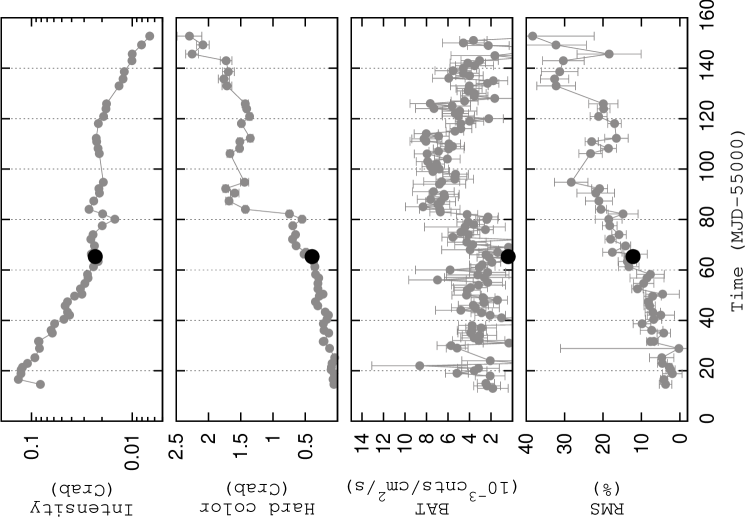
Figure 1: From top to bottom: Intensity (2–20 keV), Hard colour (16–20 keV/ 2–6 keV), BAT flux (15–50 keV), and fractional rms amplitude (1/128–100 Hz, full PCA band), respectively. Intensities, hard colours and fractional rms amplitudes are the average per day of each pointed PCA observation. The BAT measurements were taken from the BAT transient monitoring. The black filled circle marks the moment of the XMM-Newton observation.

3.2 Spectral state at the moment of the XMM-Newton observation

From Fig. 1 it is apparent that at the beginning of the outburst XTE J1652$-$453 was in the high/soft state, with high intensity, low hard colour, and low 1/128–100 Hz fractional rms amplitude (e.g., Méndez & van der Klis, 1997; Homan & Belloni, 2005). Around MJD 55080, there is a clear transition to the low/hard state, with a sharp increase of the hard colour, while both the BAT flux and the 1/128–100 Hz fractional rms amplitude increase slightly, but significantly. Transitions from the high/soft state to the intermediate state (soft- or hard-intermediate; Homan & Belloni, 2005; Belloni, 2010) are generally smooth transitions, and without multi-wavelength observations in combination with detailed timing analysis it is difficult to say when this transition exactly happened.

In Fig. 2 we show the hardness intensity diagram (HID) for the outburst of XTE J1652$-$453. For comparison we also show the HID of the black-hole candidate GX 339$-$4 of the 2002/2003 outburst. Both diagrams show the intensities and hard colours in Crab units, both calculated in the same manner as described in Section 2.1. In the HID of GX 339$-$4 we marked the different spectral states identified by Belloni et al. (2005) and Homan & Belloni (2005). Suggested by Fig. 2 together with the 1/128–100 Hz integrated rms amplitude of $\sim 15$ per cent, which is too high for the soft or the soft-intermediate state, we conclude that at the moment of the XMM-Newton observation, XTE J1652$-$453 was in the hard-intermediate state.

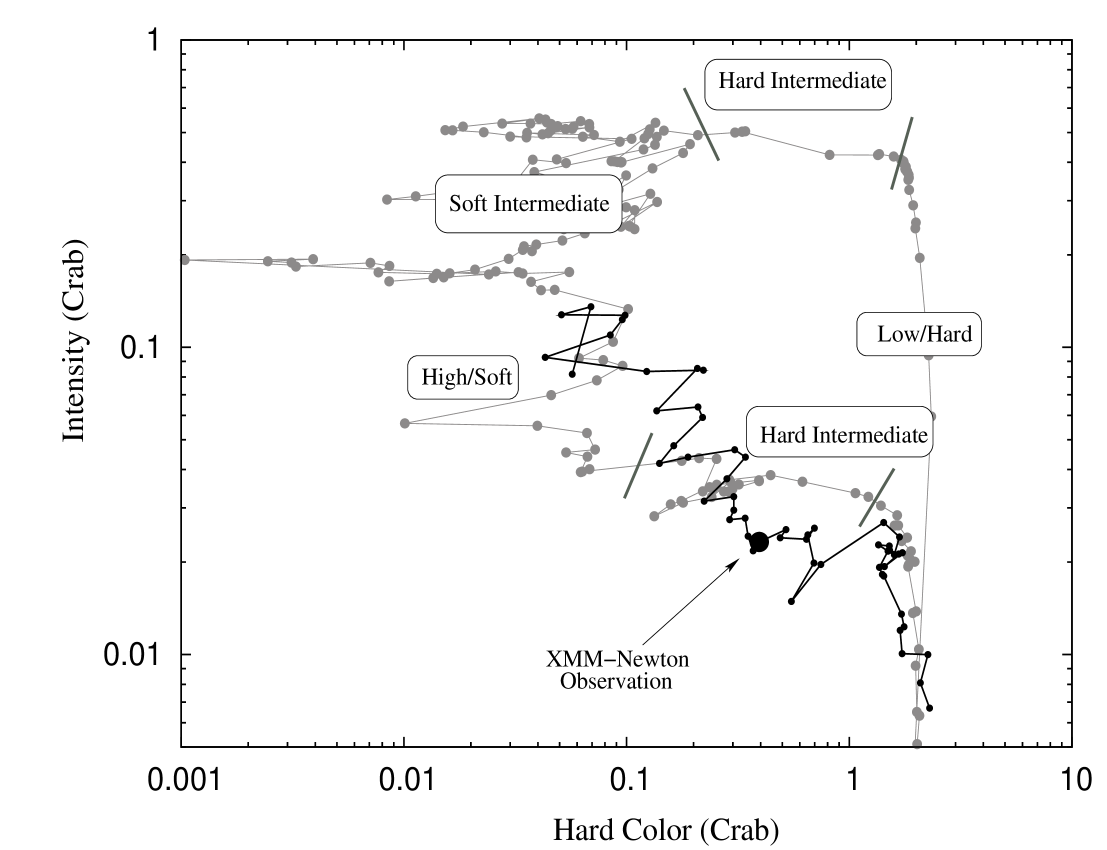
Figure 2: Hardness intensity diagram of the 2009 outburst of XTE J1652$-$453 (black), and of the 2002/2003 outburst of GX 339$-$4 (grey). Intensities and hard colours are given in Crab units (for more details see Section 2.1). For the HID of GX 339$-$4 we marked the different states identified as in Belloni et al. (2005) and Homan & Belloni (2005). We also marked the moment of the XMM-Newton observation.

3.3 Spectroscopy

For the spectral analysis of XTE J1652$-$453 we used xspec version 12.5.1 (Arnaud, 1996). Since XMM-Newton and RXTE started their observations at the same time, together with the rather constant light curve during the whole XMM-Newton observation, we fit the XMM-Newton and RXTE spectra simultaneously. We initially used a continuum model including a power law (powerlaw in xspec) and a disc blackbody (diskbb; Mitsuda et al., 1984). We included a multiplicative factor in our fit to account for differences in the absolute flux calibration between the different instruments, and to account for interstellar absorption we used the photoelectric absorption component phabs, assuming cross sections of Verner et al. (1996) and abundances of Wilms et al. (2000). (In the appendix we show how the choice of cross sections and abundances may affect the parameters.)

A strong and broad emission line at around 6–7 keV was apparent in the spectra, most likely due to Fe fluorescence lines (of neutral or ionised Fe), and we initially fit the line with a Gaussian. However, a Gaussian line did not provide a good fit ($\chi_{\nu}^{2}\simeq 2.6$); the Gaussian fit a large part of the line between 6–7 keV, but it was not able to fit the red wing extending down to 4–5 keV. Guided by the asymmetric profile, we fit the line with a relativistic line profile (e.g., for a Kerr-metric: Laor; Laor, 1991). We tried different line and continuum components to test whether the line parameters depend on the choice of line and/or continuum model. Details and results of this can be found in Section 3.3.2.

When fitting the XMM-Newton/RXTE spectra, several features appeared in the fitting residuals. Some of them are due to calibration issues of XMM-Newton data in timing mode, some of them are caused by cross-calibration issues between the different instruments, and others might be real. We discuss these features individually in the following Section.

Unless stated differently, all uncertainties given in this paper are at a 90 per cent confidence level ($\Delta\chi^{2}=2.71$), and upper limits are given at a 95 per cent confidence level. The equivalent widths (EW) of emission and absorption features are both quoted with positive values.

3.3.1 Instrumental/Cross-calibration issues

Here we list all features and issues that arose during our spectral analysis which are most likely related with uncertainties in the (cross) calibration of the different instruments.

Excess at $\sim 1$ keV:

When we fit the PN spectrum in the 0.7–11 keV range with a line and continuum model, phabs(powerlaw + diskbb + Laor), we found a strong and broad emission feature at $\sim 1$ keV, extending up to $\sim 1.3$ keV (see Fig. 3). The $\sim 1$ keV excess was also apparent in the MOS2 data, although the profile of the excess was different. Since both detectors showed this excess we cannot discard that it may be real, and we considered the possibility that it might be due to blurred Fe-L or Ne-X emission lines (see Fabian et al., 2009). We tried to fit this excess with either a Gaussian component or a relativistic line profile, but none of these models gave a good fit. No excess at $\sim 1$ keV was apparent in the RGS data, although the lower effective area does not allow us to discard it completely.

Figure 3: An excess at $\sim 1$ keV is apparent in the PN spectrum of XTE J1652$-$453. We show the data/model ratio when we fit the data with a phabs(powerlaw + diskbb + Laor) model. The spectrum is not corrected for background, and instrumental residuals are still present.

Similar excesses at $\sim 1$ keV have been seen in other sources observed with PN operated in timing mode (e.g., Martocchia et al., 2006; Sala et al., 2008; Boirin et al., 2005). The excess appears in that part of the spectrum where the flux drops abruptly due to interstellar absorption, and the EW of the excess appears to increase as a function of this absorption (see e.g., Done & Díaz Trigo, 2009). Given this, a calibration issue related with the redistribution matrix of the timing-mode data cannot be excluded at the moment. Due to the uncertain origin of this excess (a thorough investigation is beyond the scope of this paper), we ignored the EPIC data below 1.3 keV and included the RGS data to cover the spectrum below that energy.

Energy-dependent discrepancy between PCA and PN:

Fitting the PCA data in the 3–20 keV range shows an energy-dependent deviation between the PN and PCA spectra below $\sim 7$ keV. (With respect to the PN data, the PCA data show an excess that increases with decreasing energy.) Fitting the PN and PCA spectra individually (in the 1.3–11 keV and 3–20 keV ranges, respectively), there is a discrepancy in the power-law photon index, which is most likely due to a mismatch in cross-calibration between the PN and PCA instruments. To avoid the effects of this apparent energy-dependent discrepancy between PN and PCA data, in the rest of our analysis we only used PCA data in the 7–20 keV range.

Absorption features:

The fit residuals of the phabs(powerlaw + diskbb + Laor) model to the EPIC data show two absorption features at around $1.8$ and $2.1$ keV, consistent with the Si-K (1.84 keV) and Au-M (2.21 keV) edges, which are most likely of instrumental origin. To reduce the impact of these lines, we could fit each of them with a Gaussian absorption component at $1.85\pm 0.01$ and $2.13\pm 0.02$ keV, and widths of $55\pm 5$ eV and $110\pm 10$ eV, respectively, although some residuals between $\sim 1.8$–2.2 keV still remained, probably due to problems with the gain and the CTI correction. In order to keep the model as simple as possible, instead of fitting these two instrumental features with absorption components, we ignored all energy channels between 1.75–2.25 keV so that these instrumental edges will not affect the results of the analysis. However, we caution that the edges, if caused by residual problems of the CTI correction, indicate that a slight energy shift may appear in the whole energy band (see XMM-Newton Calibration Documentation XMM-SOC-CAL-TN-0083, on http://xmm.vilspa.esa.es/docs/documents/).

The RGS data showed an absorption feature at $\sim 1.4$ keV. In case we fit this absorption line with a gabs component, the best-fitting line energy is $1.42\pm 0.06$ keV, line width $\sigma=70\pm 10$ eV, and EW of $\sim 35$ and $\sim 62$ eV for RGS1 and RGS2, respectively. The width and strength of this absorption feature suggest that it is most likely due to a mismatch in the spectrum curvature of the PN and RGS data. In the rest of the analysis we fit this absorption line with a gabs component.

Further, the EPIC fit residuals above 6 keV showed additional features in the PN spectrum at high energy (see Fig. 4). The slight increase at $\sim 8.3$ keV (and the consequent dip at higher energies) is probably due to the emission lines in the detector background (see Fig. 7). Since the absorption feature at $\sim 8.7$ keV is only apparent in the PN data, and not in the MOS2 or PCA data, it is most likely an effect of not correcting for the background emission lines in the PN detector. To improve the fit statistics, we fit the absorption line at $8.78\pm 0.07$ keV, with width $\sigma=70\pm 20$ eV and EW of $37\pm 10$ eV.

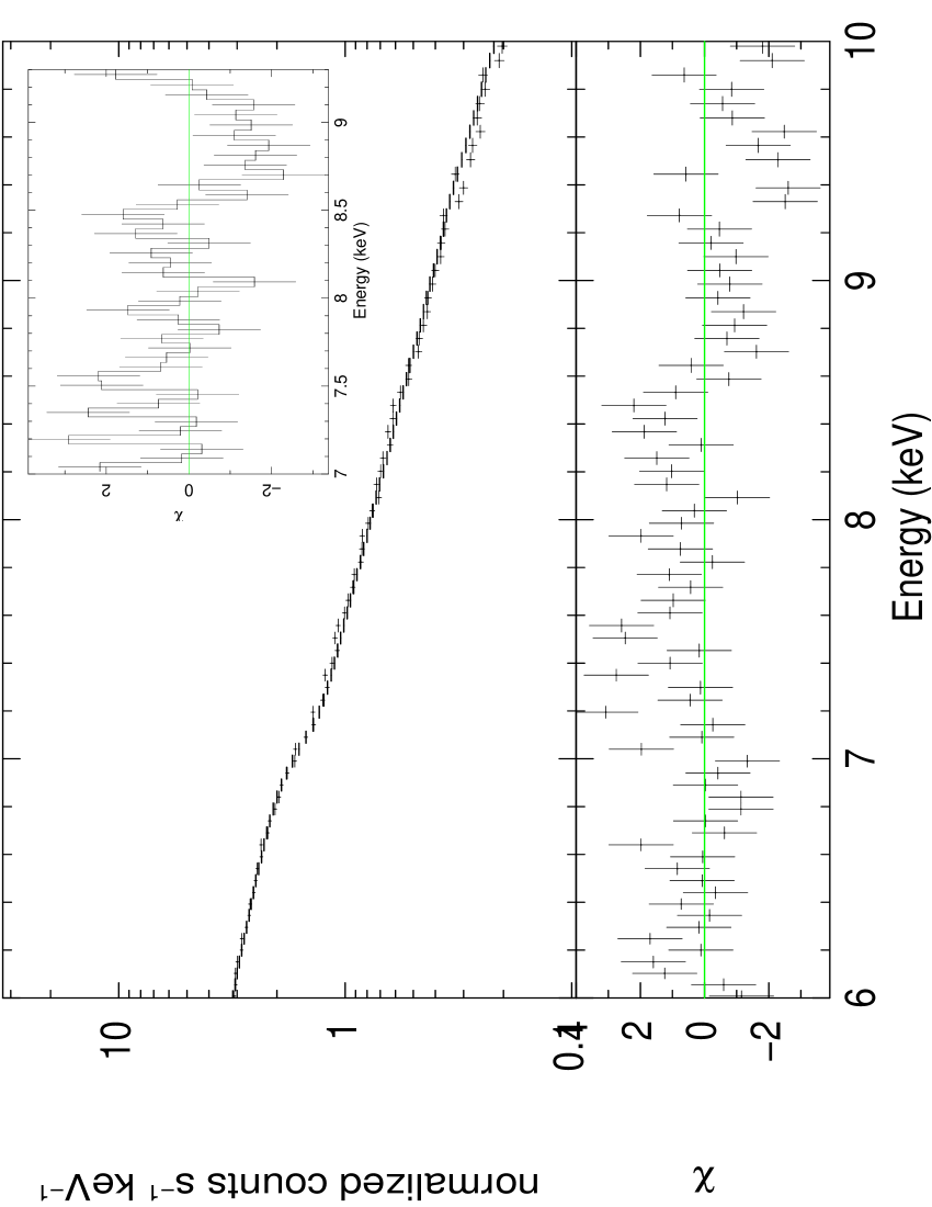
Figure 4: Zoom in of the PN spectrum of XTE J1652$-$453. The absorption feature at $\sim 9.2$ keV is apparent in the lower panel, where we show the residuals when fitting the data with the phabs(powerlaw + diskbb + Laor) model. In the sub-panel we show a zoom in of the residuals to show the apparent absorption features at $\sim 8.5$–9 keV.

In contrast to all above mentioned absorption features, the dip at $\sim 9.2$ keV could be real since both PN and PCA spectra show this feature. Since the highly ionised Fe line should be accompanied by an associated edge, we fit this feature with an edge component, and found a best-fitting edge depth of $\tau_{max}=0.20\pm 0.02$ at an energy of $9.05^{+0.12}_{-0.07}$ keV, midway between the He and H-like edges of Fe at $\sim 8.83$ and $\sim 9.28$ keV, respectively. For PCA data only, the best-fitting $\tau_{max}=0.19\pm 0.04$ at an energy of $9.14\pm 0.17$ keV, consistent with the edge of H-like Fe.

3.3.2 Line and Continuum models

For testing different line and continuum models, we simultaneously fit PN in the 1.3–11 keV range (excluding the 1.75–2.25 keV range), RGS in the 0.4–2 keV range, PCA in the 7–20 keV range, and HEXTE in the 20–150 keV range. From the available XMM-Newton/EPIC data we only included PN data since this is the best calibrated instrument in timing mode, but for a consistency check we also fit the MOS2 data separately (see Section 3.3.3).

Different relativistic line profiles:

The broad and skewed Fe emission line profile that is apparent in the spectra of XTE J1652$-$453 (see Fig. 5) is consistent with what is expected from relativistic effects, and we therefore fit it with the commonly used line profiles for a non-rotating (diskline; Fabian et al., 1989) and a maximally rotating black hole (Laor). Both line components have similar parameters: line energy, $E_{L}$, which depends on the ionisation stage of Fe, inner disc radius, $R_{\rm in}$, outer disc radius, $R_{\rm out}$, disc inclination, $\theta$, and emissivity index, $\beta$, which is the power-law dependence of the disc emissivity that scales as $R^{-\beta}$. The normalisation of the line, $N_{\rm L}$, gives the number of photons cm^-2 s^-1 in the line. We let all parameters free, except $R_{\rm out}$ which we fixed to 400 $GM/c^{2}$ (with $G$ and $c$ the usual physical constants, and $M$ the mass of the black hole). We further constrained the line energy to the range between 6.4–6.97 keV, since this is the expected range for neutral to hydrogen-like Fe-K$\alpha$ lines.

The fit with the diskline component did not provide a good fit with $\chi^{2}_{\nu}\sim 1.5$ for 362 d.o.f., with strong residuals below 6 keV, and the inner radius pegged at 6 $GM/c^{2}$. Since the diskline appears not to be the right model to describe the line, we do not further mention any results for this model. The Laor profile however, gives an acceptable fit with $\chi^{2}_{\nu}\sim 1.2$ for 362 d.o.f. In Table 1 we show the best-fitting parameters for the model with Laor, with a diskbb and powerlaw as our continuum. In the rest of the paper we refer to the phabs(diskbb + powerlaw + Laor) model as Model 1. The continuum parameters are the power-law photon index, $\Gamma$, power-law normalisation, $N_{\rm\Gamma}$ (in photons keV^-1 cm^-2 s^-1 at 1 keV), equivalent hydrogen column density, $N_{\rm H}$, temperature at the inner disc radius, $kT_{\rm in}$, and the disc blackbody normalisation, $N_{\rm dbb}=[(R_{\rm in}$/km)/($D$/10 kpc)$]^{2}\cos\theta$, where $R_{\rm in}$ is the apparent inner disc radius, $D$ the distance to the source, and $\theta$ the angle of the disc.

The broadband spectrum of XTE J1652$-$453 and the fit residuals for Model 1 are shown in the left panel of Fig. 5, with in the inset the residuals in the Fe line region when fitting the underlying continuum spectrum with Model 1 (except the line component) and excluding the Fe line band, i.e., the 4–7 keV range. In the right panel of Fig. 5 we show the unfolded spectrum and the model components of Model 1.

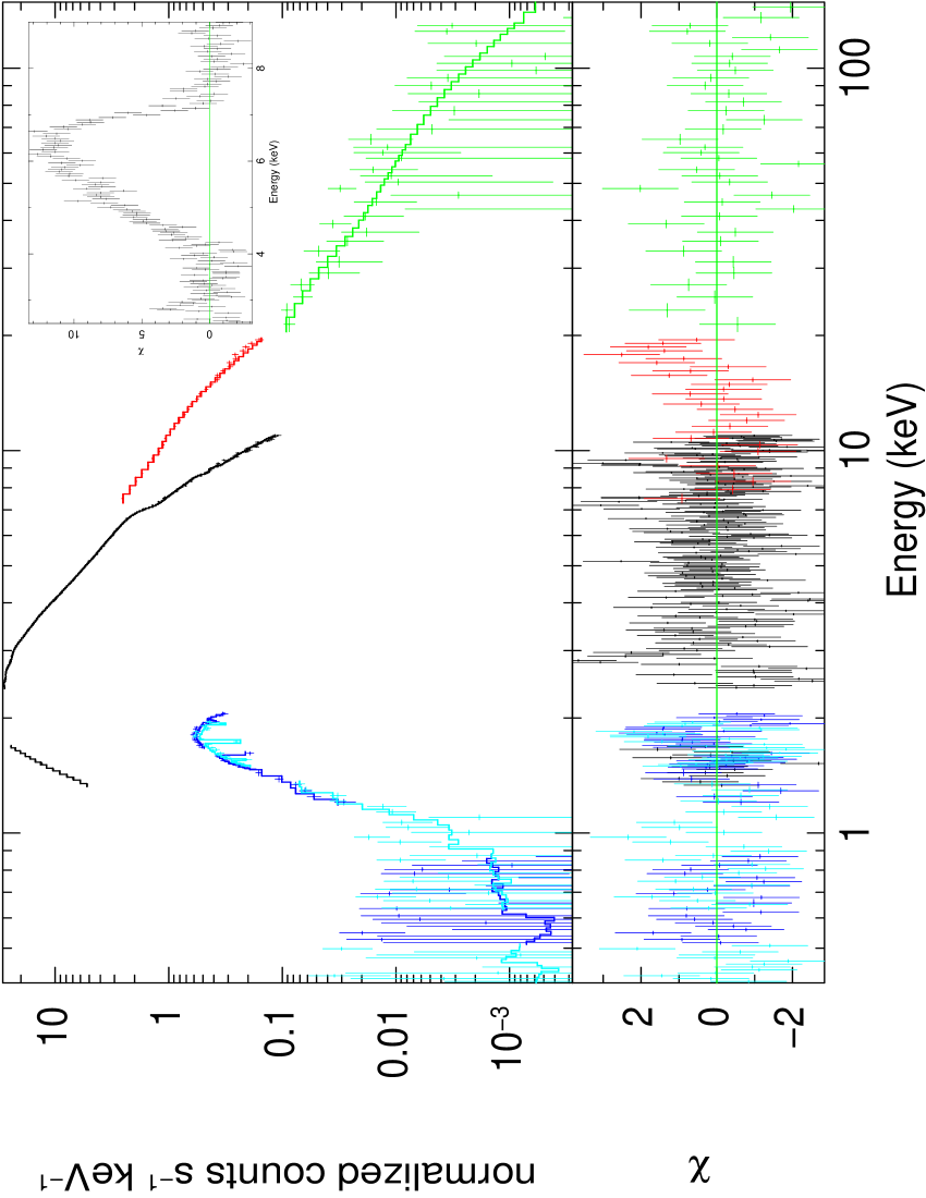
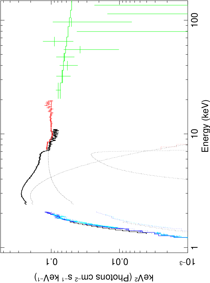
Figure 5: Left: XMM-Newton/RXTE spectra of XTE J1652$-$453: RGS (0.4–2 keV, blue), PN (1.3–11 keV, black), PCA (7–20 keV, red), and HEXTE (20–150 keV, green) with, in the bottom panel, the best-fitting residuals of Model 1. In the sub-panel in the upper-right corner we show the residuals in the Fe line region when fitting the underlying continuum spectrum with Model 1 (without Laor) and excluding the Fe line band, i.e., the 4–7 keV range. Right: Unfolded XMM-Newton/RXTE spectra of XTE J1652$-$453 and the model components (Model 1). For plotting purposes we binned the HEXTE data by a factor or 4.

Since the Laor profile assumes a maximally spinning black hole, we also tried a relativistic line profile that allows to fit for the black hole spin (kyrline, up-dated version, private communication with M. Dovčiak, but see also, Dovčiak et al., 2004). Besides the black hole angular momentum, $a/M$, the kyrline parameters are $\theta$, $R_{\rm in}$, $R_{\rm out}$, $E_{\rm L}$, and $N_{\rm L}$, which are the same parameters (and same units) as for Laor. We fixed $R_{\rm out}$ to 400 $GM/c^{2}$ and left all other parameters free. Further, within kyrline it is possible to set the directionality law for the emission (e.g., isotropic or Limb darkening/brightening), and to have a broken power-law radial emissivity profile. We assumed a disc with a single emissivity index, where $\beta$ was free to vary. We further assumed a transfer function including Laor’s limb darkening, and we only included emission from outside the marginally stable orbit. We fit kyrline using the same continuum as before, which is our Model 2: phabs(diskbb + powerlaw + kyrline). The best-fitting parameters for this model are also given in Table 1.

From Table 1 (columns 1 and 2) and Fig 5 we can see that the spectrum of XTE J1652$-$453 is well described by three components. The spectrum shows a significant contribution of thermal emission coming from a disc with a temperature of $\sim 0.6$ keV, where the disc fraction is $\sim 75$ per cent. The spectrum has significant hard emission up to at least 40 keV, where the hard tail is described by a power law with a photon index of $\sim 2.2$. We further find that that the column density of interstellar matter in the direction of XTE J1652$-$453 is $\sim 7\times 10^{22}$ cm^-2, which absorbs most of the X-rays coming from the disc. From Fig. 5 it is clear that there is a strong asymmetric Fe emission line with a red wing extending down to about 4 keV. From fits with the relativistic line profiles we find a line that is more than $15\sigma$ significant (based on the $1\sigma$ error of the line flux), and a best-fitting line energy of 6.97 keV. Despite the fact that the kyrline model is more complex (having more parameters to fit for) and has a better grid resolution (more steps over which the line is integrated) than the Laor component, the inferred line parameters for both profiles are still consistent. From both relativistic line profiles we find that the disc is observed at a low inclination, $<20^{\circ}$, and has an inner disc radius of $\sim 3.5$ $GM/c^{2}$. From the kyrline profile we find that the Fe emission line is indicative of a fast spinning black hole, although it is also consistent with a moderately spinning black hole, with a spin parameter of $\sim 0.45$.

Different continuum models:

As shown in previous work (see e.g., Hiemstra et al., 2009), the choice of continuum model can affect the parameter values of the line and other continuum components, affecting any physical interpretation. To investigate the effect of the continuum on the inferred line profile, we tested different continuum components. Given that the best-fitting line parameters are consistent between the fits with a Laor or a kyrline component, we used the Laor profile to model the Fe emission line since it gives a slightly better fit, and it is computational much faster than kyrline.

I: cutoffpl
We first tried to fit the hard emission with a cutoffpl component to see whether there is an exponential roll-off at high energy. However, we did not find a roll-off in the hard power-law tail within the energy coverage of our data. Therefore, using a cutoffpl is effectively the same as using a powerlaw component.

II: CompTT
Next (Model 3), we replaced the powerlaw component in Model 1 with a component that describes the hard emission as thermal Comptonisation of soft photons in a hot plasma (CompTT; Titarchuk, 1994), where we assumed a disc geometry for the Comptonising plasma. The parameters of CompTT are the input soft photon (Wien) temperature $T_{0}$, the plasma temperature $kT$, the plasma optical depth $\tau$, and the normalisation $N_{\rm Comp}$. The best-fitting results for Model 3 are given in Table 1.

We find that the spectrum of XTE J1652$-$453 is well described by a thermal component and a Comptonising component, where the Comptonising plasma is hot ($kT\sim 170$ keV) and optically thin ($\tau\ll 1$). Because of the low-energy cutoff at the seed photon energy, the unabsorbed 0.5–10 keV flux of the CompTT component is $\sim 2$–3 times lower than the flux of the powerlaw component in Models 1 and 2. Due to this cutoff, the hard power-law tail does not contribute to very low energies and causes the slightly lower value for $N_{\rm H}$, and thus a slightly higher contribution of the disk component. The other parameters are consistent with the values obtained in Models 1 and 2.

III: CompPS
Subsequently, we tried a component that describes a hybrid thermal/non-thermal Comptonising plasma (CompPS; Poutanen & Svensson, 1996). This model component computes the Comptonisation spectra taking into account the geometry and optical depth of the corona, the spectral distribution of soft seed photons, and the parameters of the electron distribution. The resulting spectrum includes the incident thermal emission, the Comptonized emission, and the Compton reflection. For the source of soft seed photons (the incident thermal emission) we assumed a multicolor disk blackbody, and we therefore did not include a separate diskbb component to the model. Since we only wanted to test how a hybrid plasma affects the line and continuum parameters, we did not include the Compton reflection in CompPS, but we still added a Laor component to fit the Fe line. For a spherical geometry of the corona, the best-fitting results for this model (Model 4) are given in Table 1. The free parameters are the electron temperature of the corona, $kT_{e}$, seed photon temperature, $kT_{dbb}$, optical depth of the corona, $\tau$, and normalization, $N_{CPS}$, which has the same units as the diskbb normalization. We further fixed the power-law index of the energy distribution of the non-thermal electrons to 2, we set the minimum and maximum lorentz factors of the non-thermal electrons to 2 and 3000, respectively, and set the abundances to solar.

We find that Model 4 fits the data well with $\chi^{2}_{\nu}\sim 1.2$ for 362 d.o.f. The hybrid Comptonising plasma has a best-fitting temperature of $\sim 75$ keV and is optically thin ($\tau\sim 0.15$). The hybrid plasma is cooler than the fully thermal plasma in Model 3, while the optical depth is a factor 2 larger. We further find that the parameters of the disk and line are hardly affected by the choice of the Comptonising component (non-thermal, Model 1, thermal, Model 3, or hybrid, Model 4), with values being consistent within errors. However, the equivalent width is $\sim 10$–20 per cent lower in Model 4 than in the other 2 models.

IV: reflionx
Since the line energy of the Fe emission line suggests a high ionisation stage of Fe, we tried an ionised reflection model (reflionx; Ross & Fabian, 2005). This model describes the reflection off an ionised and optically-thick atmosphere of constant density (such as the surface of an accretion disc) that is illuminated by radiation with a power-law spectrum. Since reflionx only provides the reflected emission, we included a powerlaw component to account for the direct emission. We coupled the photon index of the illuminating power-law component in reflionx to the photon index of the powerlaw. reflionx includes ionisation states and transitions from the most important ions, like O III-VIII, Fe VI-XXVI, and several others. To account for relativistic effects in the disc, we used a relativistic convolution component (Kerrconv; Brenneman & Reynolds, 2006). All together, Model 5 was phabs(diskbb + powerlaw + Kerrconv$\ast$reflionx) model. For this continuum model the absorption component at $\sim 8.7$ keV was not significant anymore and we therefore took it out. The absorption component at $\sim 1.4$ keV and the edge at $\sim 9.2$ keV were still included. The free parameters in the reflionx model are the ionisation parameter, $\xi$ (where $\xi=4\pi F/n$, with $F$ the total illuminating flux and $n$ the hydrogen number density), and the normalisation, $N_{\rm ref}$. We initially also let the Fe abundance to be free, finding a best-fitting value of 4 times solar. This is unlikely for a low-mass X-ray binary, and we therefore fixed the Fe abundance to solar. For Kerrconv, we assumed a single emissivity index, which was free to vary. The black hole spin and inclination angle of the disc were also free parameters. We further fixed the inner radius of the disc to be equal to the radius of the marginally stable orbit, $R_{\rm ms}$, and the outer radius to 400 $R_{\rm ms}$. The best-fitting parameters for Model 5 are also given in Table 1.

We find that Model 5 fits the overall continuum and Fe emission line quite well, except that a clear absorption feature remained in the residuals at $\sim 7.1$ keV, causing a slightly higher $\chi^{2}_{\nu}$ compared with Models 1–3. Although this absorption feature is not obviously apparent in the raw data, we checked whether it can be either a K-edge of neutral Fe (7.11 keV), a blue-shifted absorption line of highly ionised Fe, or a mismatch in the model used to describe the data. We tried to fit the residuals at $\sim 7.1$ keV with an edge component, but since the feature is narrow, an edge does not provide a good fit. When we fit the residuals with a gabs component, the best-fitting absorption line has a central energy of 7.2 keV and a width of 0.1 keV. For the case of a blue-shifted Fe-XXVI Ly-$\alpha$ line, the blue shift corresponds to a velocity of $\sim 9500$ km s^-1, which is significantly higher than the blue shift of $\sim 300$–1600 km s^-1 observed in GRO J1655$-$40 (Miller et al., 2006). For other Fe lines the blue shift would be even larger. Since reflionx self-consistently incorporates Compton scattering, the Fe feature in this model has an extended blue wing up to $\sim 8$ keV, whereas the observed Fe emission line in the spectrum of XTE J1652$-$453 shows a sharp drop at $\sim 7$ keV. We therefore conclude that the negative residuals at $\sim 7.1$ keV are likely caused by a deficiency in the model (see Done & Gierliński, 2006).

From Model 5 we find a high ionisation parameter, $\xi\sim 2900$ erg cm s^-1, indicating that the emission line is dominated by highly ionised Fe, which is consistent with the line energy of 6.97 keV that we inferred for the relativistic line profiles in Models 1–3. We also find a moderately spinning black hole with a spin parameters of $\sim 0.5$, consistent with the lower confidence value inferred from Model 2. Further, the best-fitting inclination is consistent with that inferred from Laor, while the best-fitting emissivity index is slightly lower than we found from Models 1–3. The powerlaw component in Model 5 only represents the direct emission, and therefore its normalisation is $\sim 2$ times lower than for the other three models. All other parameters of Model 5 are consistent with those inferred for the other models. The reflection fraction for Model 5, as estimated from the (0.5–150 keV) flux ratio between the reflected and incident emission, is $\sim 90$ per cent.

Table 1: Different line and continuum models fit to XMM-Newton/RXTE data of XTE J1652$-$453

Model component	Parameter	Model 1	Model 2	Model 3	Model 4	Model 5
phabs	$N_{\rm H}$ ($10^{22}$)	6.73$\pm$0.01	6.75$\pm$0.02	6.66$\pm$0.01	6.71$\pm$0.02	6.73$\pm$0.01
diskbb	$kT_{\rm in}$ (keV)	0.59$\pm$0.01	0.59$\pm$0.01	0.60$\pm$0.01	–	0.59$\pm$0.01
	$N_{\rm dbb}$	1015${}^{+36}_{-11}$	1051$\pm$40	1090${}^{+16}_{-36}$	–	998$\pm$10
	Flux ($10^{-9}$)	2.09$\pm$0.07	2.12$\pm$0.08	2.37${}^{+0.20}_{-0.08}$	–	2.08$\pm$0.02
powerlaw	$\Gamma$	2.23$\pm$0.03	2.22$\pm$0.03	–	–	2.16$\pm$0.02
	$N_{\rm\Gamma}$	0.18$\pm$0.01	0.18$\pm$0.01	–	–	0.09$\pm$0.01
	Flux ($10^{-9}$)	0.74$\pm$0.06	0.73$\pm$0.05	–	–	0.39$\pm$0.04
CompTT	$T_{0}$ (keV)	–	–	0.88${}^{+0.12}_{-0.03}$	–	–
	$kT$ (keV)	–	–	170${}^{+24}_{-51}$	–	–
	$\tau$	–	–	0.06$\pm$0.01	–	–
	$N_{\rm Comp}$ ($10^{-4}$)	–	–	3.25${}^{+9.31}_{-1.12}$	–	–
	Flux ($10^{-9}$)	–	–	0.27${}^{+0.77}_{-0.09}$	–	–
CompPS	$kT_{e}$ (keV)	–	–	–	75.3$\pm$1.3	–
	$kT_{dbb}$ (keV)	–	–	–	0.58$\pm$0.01	–
	$\tau$	–	–	–	0.15$\pm$0.01	–
	$N_{CPS}$	–	–	–	1314$\pm$37	–
	Flux ($10^{-9}$)	–	–	–	2.72${}^{+0.12}_{-0.03}$	–
Laor	$E_{\rm L}$ (keV)	6.97${}^{+0}_{-0.02}$	–	6.97${}^{+0}_{-0.06}$	6.97${}^{+0}_{-0.02}$	–
	$\beta$	3.4$\pm$0.1	–	3.4$\pm$0.1	3.3$\pm$0.1	–
	$R_{\rm in}$ ($GM/c^{2}$)	3.65${}^{+0.31}_{-0.02}$	–	3.64${}^{+0.27}_{-0.03}$	4.01${}^{+0.18}_{-0.10}$	–
	$\theta$ (deg)	9.4${}^{+4.5}_{-3.8}$	–	9.4$\pm$3.9	5.3${}^{+3.3}_{-5.3}$	–
	$N_{\rm L}$ ($10^{-3}$)	1.6$\pm$0.1	–	1.6$\pm$0.1	1.3$\pm$0.1	–
	EW (eV)	455${}^{+17}_{-26}$	–	451${}^{+21}_{-28}$	366${}^{+21}_{-15}$	–
kyrline	$a/M$ ($GM/c$)	–	0.96${}^{+0.01}_{-0.51}$	–	–	–
	$E_{\rm L}$ (keV)	–	6.97${}^{+0}_{-0.04}$	–	–	–
	$\beta$	–	3.5$\pm$0.1	–	–	–
	$R_{\rm in}$ ($GM/c^{2}$)	–	3.39${}^{+0.31}_{-0.19}$	–	–	–
	$\theta$ (deg)	–	16.6$\pm$3.0	–	–	–
	$N_{\rm L}$ ($10^{-3}$)	–	1.8$\pm$0.2	–	–	–
	EW (eV)	–	470${}^{+28}_{-41}$	–	–	–
reflionx	$\xi$ (erg cm s-1)	–	–	–	–	2872${}^{+807}_{-26}$
	$N_{\rm ref}$ ($10^{-7}$)	–	–	–	–	4.9${}^{+0.04}_{-0.23}$
Kerrconv	$a/M$	–	–	–	–	0.45$\pm$0.02
	$\beta$	–	–	–	–	2.7$\pm$0.1
	$\theta$ (deg)	–	–	–	–	8.8$\pm$0.1
	$\chi^{2}_{\nu}$ ($\chi^{2}/\nu$)	1.22 (422.2/362)	1.25 (451.1/361)	1.21 (437.2/360)	1.23 (445.2/362)	1.26 (460.2/365)
	Total Flux ($10^{-9}$)	2.84$\pm$0.04	2.87$\pm$0.03	2.65${}^{+0.76}_{-0.09}$	2.73$\pm$0.02	2.86$\pm$0.11
NOTES.– Results are based on spectral fits to RGS/PN/PCA/HEXTE data in the 0.4–150 keV range. Columns 1–2 give the results of
different relativistic line models using the continuum model phabs(diskbb + powerlaw) with line profiles Laor (Model 1) and  kyrline (Mo-
del 2). Columns 3–5 give the results of different continuum models. Models 3 and 4, respectively, include a thermal Comptonising plasma
(CompTT) and a hybrid plasma (CompPS) to model the hard emission, and the Laor component is used to fit the Fe line. For Model 4 the
Comptonising spectrum self-consistently includes the incident thermal emission, so we did not include a separate diskbb component as we
did for Model 3.  Model 5 is the continuum model phabs(diskbb + powerlaw + Kerrconv$\ast$reflionx), where reflionx describes the reflected
emission, powerlaw models the direct emission, and Kerrconv smears for relativistic effects. For details about parameters, see text. Cross-
calibration constants for the different instruments with respect to PN are: 1.09 (PCA), 0.84 (RGS1 & HEXTE), and 0.79 (RGS2). Fluxes
are unabsorbed and given for the 0.5–10 keV range in units of erg cm-2 s-1.

3.3.3 Consistency check: MOS2 data

For consistency, we verified our results obtained from fits to the RGS/PN/RXTE data (in this section simply referred to as PN data) with fits to the RGS/MOS2/RXTE data (and hence referred to as MOS2 data). For comparison we only fit Model 1 to the MOS2 data, assuming the same abundances, cross sections, and energy ranges that we used to fit the PN data (see Section 3.3). We ignored the MOS2 channels between 1.75–2.25 keV for similar reasons as for PN, added a Gaussian absorption component to fit the $\sim$1.4 keV feature seen in the RGS spectra, and fit the $\sim 9.2$ keV feature in MOS2 with an edge.

Model 1 (including all above absorption features) fit the MOS2 data well with $\chi^{2}_{\nu}=1.25$ (458.0/366). The unabsorbed 0.5–10 keV flux is $2.3\times 10^{-9}$ erg cm^-2 s^-1, and the best-fitting parameters for the continuum components are $N_{\rm H}=(6.77\pm 0.05)\times 10^{22}$ cm^-2, $kT_{\rm in}=0.60\pm 0.01$ keV, $N_{\rm dbb}=859^{+59}_{-47}$, $\Gamma=2.17\pm 0.05$, and $N_{\Gamma}=0.13\pm 0.02$ photons keV^-1 cm^-2 s^-1 at 1 keV. For the Fe line the best-fitting values are $E_{\rm L}=6.97^{+0}_{-0.51}$ keV, $R_{\rm in}=2.8\pm 0.5$ $GM/c^{2}$, $\beta=3.7\pm 0.4$, $\theta=25^{+18}_{-6}$ degrees, and $N_{\rm L}=1.9\pm 0.5\times 10^{-3}$ photons cm^-2 s^-1 in the line. The Fe emission line has an EW of $514^{+100}_{-75}$ eV consistent with that obtained from PN data. The edge at $\sim 9.2$ and the absorption feature at $\sim 1.4$ keV have parameters which are consistent with the values obtained from the PN data.

We find that most of the continuum and line parameters obtained from the MOS2 data are consistent (within errors) with the values obtained from the PN data. The only parameters that were not consistent are the diskbb normalisation and the inclination. However, the inclination inferred from the MOS2 data is consistent (within errors) with the inclination deduced from the kyrline profile that we fit to the PN data. The diskbb normalisation obtained from fits to the MOS2 data is lower than that for PN, which is most likely due to the fact that we subtracted the background spectrum in the case of the MOS2 data, but we did not for the PN data.

3.4 Other possible broadening mechanisms

By using the Laor and kyrline components in our Models 1–4 we are in fact assuming that the line is only broadened by relativistic effects. However, one should consider the possibility that other mechanisms contribute to the total line width. Besides broadening due to thermal Comptonisation by the disk, as in reflionx (see Section 3.3.2), an alternative mechanism could be Compton broadening due to electron scattering in the hot plasma above the accretion disc (Czerny et al., 1991). The width of a Compton scattered line depends on the temperature and the optical depth of the Comptonising plasma. For a single Compton scattering $\sigma_{\rm E}/E=[(2kT_{\rm e})/(m_{\rm e}c^{2})]^{1/2}$, with $\sigma_{\rm E}$ the line width, $E$ the central line energy, $kT_{\rm e}$ the electron temperature of the plasma, and $m_{\rm e}$ and $c$ the usual physical constants (Pozdnyakov et al., 1983). From fits including a CompTT component to describe the high-energy emission (Model 3), we find $\tau\simeq 0.06$ and $kT_{\rm e}\simeq 170$ keV (see Table 1), which means that the Comptonising plasma would only intercept a fraction of 0.06 of the line photons, and scatter these into a broader line of width $\sim 5.5$ keV. A fraction of 0.94 of the line is unaffected, and comes out at its intrinsic width. Thus the line would have a predominantly narrow core, but with 6 per cent of the photons scattered to such extent that it would be difficult (or even impossible) to distinguish from the continuum. However, as a matter of fact the problem here is that in all probability the Comptonisation is not thermal but instead is non-thermal. Therefore the obtained optical depth and temperature are not real. As we found from the fits of a hybrid Comptonisation model (Model 4), the plasma can also be cooler ($kT_{\rm e}\simeq 75$ keV), but we still found a low optical depth ($\tau\sim 0.15$). In this case $\sim 15$ per cent of the line photons will be scattered into a broader line of width $\sim 3.5$ keV, which is still too broad and too weak to be distinguished from the continuum.

Kallman & White (1989) showed that the apparent widths of Fe lines may be due to a blend of narrow line components arising from different ionisation states, with each of these narrow components in turn affected by Compton broadening. The combination of blending and Compton broadening produces a line profile with an equivalent width, line width and line energy that depend on several factors, besides the ionisation parameter of the emitting gas. In this scenario, the total line width is not only set by relativistic effects, but also by the combined effects of gas motions (rotation), Compton scattering, and blending of emission of several ionisation states, where the centroid line energy is a function of the degree of ionisation of Fe, and hence the ionisation parameter of the emitting gas (Kallman & White, 1989). To estimate the effect of line blending, we fit the Fe line with a multi-component line model. Assuming the continuum of Model 1, we added three Laor components with the line energies fixed at 6.4, 6.7 and 6.97 keV, for neutral, He-like, and H-like Fe, respectively. We fixed the outer radius of the disc to 400 $GM/c^{2}$, and let the rest of the parameters free to vary. Except for the line normalisations, we coupled the line parameters of each of the three Laor profiles. We find that the multi-line model fits the observed Fe emission line well, $\chi^{2}_{\nu}=1.17$ for 361 d.o.f. The best-fitting parameters are $R_{\rm in}=2.20^{+0.10}_{-0.03}$ $GM/c^{2}$, $\beta=4.0\pm 0.1$, $\theta=40.7\pm 1.5$ degrees, and $N_{\rm L}=2.0\pm 0.2\times 10^{-3}$, and $0.6\pm 0.28\times 10^{-3}$ photons cm^-2 s^-1 for the 6.4 and 6.97 keV lines, respectively. The 6.7 keV line was not required by the fit, with UL to the EW of $\sim 51$ eV. The equivalent widths of the neutral and H-like Fe were $389^{+20}_{-39}$ and $127\pm 41$ eV, respectively. The best-fitting continuum parameters were consistent with the values reported for a single-line model (Model 1, Table 1). From this we initially concluded that line blending can partially explain the observed line profile, although relativistic effects are still important. The resulting disc inclination was significantly higher for the multi-line model than for the single-line model. In contrast to the single Laor profile, the multi-line model was dominated by the neutral-Fe line, with an equivalent width $\sim 3$ times higher than the one of the H-like Fe line. Based on the high ionisation parameter, $\xi\sim 2900$ erg cm s^-1, obtained from the fits with reflionx (see Table 1) we do not expect a significant fraction of neutral Fe in the disc, which casts some doubt on this approach. Moreover, given the observed high disc temperature we do not expect much neutral Fe, irrespective of photo-ionisation.

A third broadening mechanism that we considered explains the red-skewed emission line by down-scattering of line photons in an optically thick and partly ionised wind from the BH (see Titarchuk et al., 2009, and references therein). In this model the effect of photo-absorption of the line photons at higher energies (above 7–8 keV, depending on the ionisation stage of the wind) suppresses the blue wing of the Fe emission line, and therefore leads only to a redshifted profile, where the redshift of the line photons is to first order a function of $v/c$, with $v$ the outflow velocity. Contrary to the optically thick Comptonising wind assumed in this model, we find an optically thin corona for the case of XTE J1652$-$453, which makes this outflow model unlikely to explain the observed broad and red-skewed Fe line.

3.5 Timing analysis

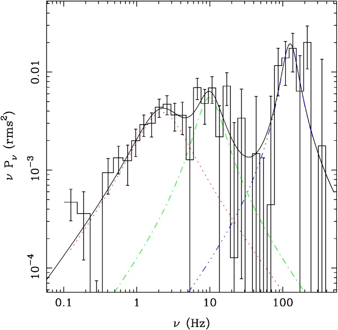
Figure 6: Power density spectrum of XTE J1652$-$453 using the RXTE/PCA data from the observation taken simultaneously with that of XMM-Newton (MJD 55065, RXTE ObsID 94432-01-04-00). The plot shows the frequency$\times$Fourier Power in units of squared rms fractional amplitude versus frequency. The black solid line is the best-fitting model to the data using three Lorentzians. The three Lorentzians are shown by the red dashed, green dot-dashed, and blue dot-dot-dashed lines, respectively.

The power spectrum of the RXTE observation that was taken simultaneously with the one of XMM-Newton,can be reasonably fit ($\chi^{2}=35.9$ for 25 d.o.f.) with three Lorentzians at $2.2\pm 0.4$ Hz, $10.0\pm 1.7$ Hz, and $131\pm 20$ Hz, respectively. (These are the frequencies at which the Lorentzians peak in the frequency$\times$power representation of e.g., Belloni et al., 2002) The single-trial significance of each Lorentzian (defined as the power of the Lorentzian divided by its negative error) was 4.9$\sigma$, 2.8$\sigma$, and 3.4$\sigma$, respectively. The three Lorentzian had, respectively, quality factors, $Q=\nu_{0}$/FWHM (where $\nu_{0}$ and FWHM are the central frequency and the full-width at half maximum of the Lorentzian) of $0.5\pm 0.2$, $1.0\pm 0.7$, and $1.5\pm 0.9$, and total fractional rms amplitudes of $8.9\pm 0.9$, $8.3\pm 1.6$, and $13.8\pm 2.2$ per cent. In Fig. 6 we show the power density spectrum of this observation, together with the best-fitting model. The black solid line is the total model, while the dashed, dotted and dashed-dotted lines in colour show the individual components.

If the marginally significant Lorentzian at $\sim 130$ Hz is real, we can use it to put an upper limit on the black-hole mass, as any frequency should be less than Keplerian. For a Keplerian frequency of $\nu\sim 130$ Hz at the inner edge of the accretion disc of $R_{\rm in}\sim 4$ $GM/c^{2}$, $\nu=c^{3}/[2\pi GM(R_{\rm in}^{3/2}+a)]$ (Bardeen et al., 1972), with $a$ the spin parameter and $M$ the mass of the black hole, we find an upper limit on the mass of $\sim 30M_{\odot}$. Given that most known BH binaries have mass around $\sim 10M_{\odot}$, then this shows that these fluctuations are indeed produced close to the black hole.

4 Discussion

The XMM-Newton/RXTE energy spectrum of XTE J1652$-$453 shows a broad and strong Fe emission line with an equivalent width of $\sim 450$ eV, which is among the strongest ever seen from a black-hole candidate (see e.g., Rossi et al., 2005; Miller et al., 2004). The line is consistent with being produced by reflection off the accretion disc, broadened by relativistic effects. The power spectrum from RXTE data can be fitted with two Lorentzians below 10 Hz, and shows an additional variability component above 50 Hz. The simultaneous XMM-Newton/RXTE observations were performed when XTE J1652$-$453 was in the hard-intermediate state (HIMS; Méndez & van der Klis, 1997; Homan & Belloni, 2005), as the outburst decayed from the disc dominated high/soft state towards the low/hard state. Our high-resolution, broadband observations substantially increase the number of good datasets from this state (Miller et al., 2004, the other is GX 339$-$4). The strong line as well as the additional component at high frequencies are both characteristic of the hard-intermediate state. Miller et al. (2004) show a Chandra grating spectrum of the black-hole candidate GX 339$-$4, with a very similar continuum spectrum as XTE J1652$-$453, where the line has an equivalent width of $\sim 600$ eV. Klein-Wolt & van der Klis (2008) show that there is an additional noise component at high frequencies in the HIMS, although it is somewhat weaker than the component seen in our data. Power spectra taken in the HIMS also typically show the strongest, most coherent, low-frequency QPO (e.g., Klein-Wolt & van der Klis, 2008). The lack of any such coherent low-frequency QPO in our data may imply that we view the system at a rather low inclination angle. This is consistent with the inclination inferred from fitting the Fe line profile with relativistic models.

Understanding the intermediate state is important as it marks the onset of the spectral transition, and the appearance of the radio jet. While there is still debate on the nature of the transition, most models currently explain it by the inner disc evaporating into a hot coronal flow (see e.g., Liu et al., 2006; Meyer et al., 2000). The intermediate state is therefore the one in which the disc is only slightly recessed from the last stable orbit, so there is strong disc emission, but there is also strong hard X-ray flux from the re-emerging hot flow. This geometry also predicts that there should be strong reflection features, and that these should be strongly smeared by relativistic effects. As the outburst declines further, the models predict that the inner disc quickly recedes, being replaced by the hot flow. With the receding disc, the solid angle subtended by the optically thick disc decreases, the amount of reflection decreases, and the larger radius means that the line is less strongly smeared. These models then suggest that the strongest and broadest Fe lines should be seen in the intermediate states, where the disc is closest to the last stable orbit, but co-exists with enough of the hard X-ray emitting corona to produce the required illumination of the disc.

From low-resolution (RXTE) spectral monitoring it is indeed seen that for the high/soft states, as there is very little hard X-ray emission illuminating the disc, the Fe lines are generally weak, while they appear strongly at the intermediate states, as coronal X-ray emission re-appear. The line width and strength then decrease as the outburst declines (Gilfanov, 2010). However, such low-resolution data cannot distinguish changes in the reflection broadening from changes in the ionisation state, and since the disc temperature and/or strength of the irradiation change, the ionisation state should also change. Even if there is no change in geometry, an increase in disc temperature gives an increase in ionisation state, and so the strength of the consequent reflection features increases (Ross & Fabian, 1993, 2007), as well as the line width increases due to increased Compton broadening (e.g., Young et al., 2005). Moderate to high resolution data show that the Fe lines are ionised in the intermediate state (e.g., Miller et al., 2004, and our data), and are predominantly neutral in the hardest low/hard state (e.g., Tomsick et al., 2009; Hiemstra et al., 2009).

The high-resolution, broadband spectrum of XTE J1652$-$453 allows us to separately constrain ionisation, solid angle and relativistic smearing. The ionisation is high with log$\xi\sim 3.5$, and the very broad Fe line requires strong relativistic effects. The fits using a self-consistent reflection model give $R_{\rm in}\simeq 4$ $GM/c^{2}$ corresponding to the last stable orbit for a black hole of spin $\sim 0.5$. This is a lower limit since we expect the disc to be slightly recessed. None the less, the RXTE monitoring of XTE J1652$-$453 shows that the direct disc emission has similar temperature and normalisation as in the high/soft state earlier in the outburst (; ), supporting the idea that the disc is very close to the last stable orbit in our data.

However, the fits with the self-consistent reflection model show clear negative residuals at $\sim 7.1$ keV. This could correspond to a blue-shifted absorption line, such as the ones that are often seen in high inclination systems (e.g., Kubota et al., 2007). This absorption feature is not obviously apparent in the raw data, and it is only required when the smeared reflionx model is used since the intrinsic Compton broadening in this model predicts no sharp drop on the blue wing of the line (Done & Gierliński, 2006). The reflionx model underestimates the Compton broadening as it calculates the temperature of the disc from irradiation only, for $kT$ of 0.1–0.3 keV (Ross & Fabian, 1993). This is obviously lower than the observed inner disc temperature of 0.6 keV. The Compton broadened line width should be $\sigma\propto E_{\rm line}\sqrt{(2kT_{e})/(m_{e}c^{2})}$ $\sim 0.32$ keV for He-like Fe. This is negligible compared to the 1.7–2 keV broadening implied by $R_{\rm in}\sim 4$ $GM/c^{2}$, and should not significantly change the derived inner radius. The Compton broadening smooths out the sharp drop from the blue wing of the line even more, and increases the mismatch with the data at $\sim 7.1$ keV. Since the model does not describe the data in detail, we should be cautious in interpreting the reflection parameters in detail.

5 Summary

We observed the black-hole candidate and X-ray transient XTE J1652$-$453 simultaneously with XMM-Newton and RXTE. During this observation the source was in the hard-intermediate state (Homan & Belloni, 2005). We found a strong and asymmetric Fe emission line in the X-ray spectrum of XTE J1652$-$453, with an equivalent width of $\sim 450$ eV, one of the strongest lines ever seen from a black-hole candidate. From fits to only XMM-Newton/PN spectrum, the equivalent width is slightly lower, $\sim 380$ eV.

The line is also broad, giving an inner disc radius of $\sim 4$ $GM/c^{2}$, from either a single Laor line profile or from a self-consistent ionised reflection model. This implies a spin parameter of $\sim 0.5$, which is a lower limit as the disc may be slightly recessed in this state. In any case, neither model fits the data well in detail. This is not at all surprising for the single Laor line as the line must be accompanied by a reflected continuum. Be that as it may, the self-consistent ionised reflection model used here incorporates all the known effects such as multiple lines and edges from the different ionisation states of Fe (and other elements), together with Compton broadening (Ross & Fabian, 2005), such that the line is intrinsically broad. The characteristic skewed profile expected from a single narrow line is smeared out, so there is no sharp drop in the model at the blue side of the line. However, the data clearly prefer such a feature, indicating that even the best current reflection models may not be able to describe the detailed shape of the Fe line seen in the spectrum of this state.

The Fourier power spectrum of the RXTE observation simultaneous with that of XMM-Newton shows additional variability above 50 Hz. No coherent QPOs at low frequency are accompanying this, which may suggest that we see the source at a fairly low inclination angle. The $3.4\sigma$ (single trial) component at $\sim 130$ Hz is too broad to be the high-frequency QPO, but in case it is, and assuming that it reflects the Keplerian frequency of the inner disc radius of $\sim 4$ gravitational radii (inferred from the line profile), then the estimated upper limit on the black-hole mass is $\sim 30$ $M_{\odot}$. None the less, since the source is in the hard-intermediate state rather than in the soft-intermediate state where the high-frequency QPOs are occasionally seen (Klein-Wolt & van der Klis, 2008), this additional high-frequency component may be a related feature at lower frequencies and lower coherence, and it might be connected to the re-emergence of the jet.

6 Acknowledgements

We thank the XMM-Newton team and the project scientist Norbert Schartel for performing the ToO observation. We also like to thank the RXTE team for rescheduling to obtain a contemporaneous observation. We are grateful to an anonymous referree for constructive comments, and we thank Juri Poutanen for a valuable discussion. PC acknowledges funding via a EU Marie Curie Intra-European Fellowship under contract no. 2009-237722

Appendix A Choice of background and abundances

A.1 Background in PN timing mode

As can be seen in Fig. 7, the PN background spectrum (red) extracted from the XTE J1655$-$453 observation, is contaminated with source photons (see Section 2.2.1 for more details about the extraction criteria). Using this background spectrum leads to an over-subtraction of the source spectrum and it may change the results of the spectral analysis. To investigate whether the continuum and line parameters are affected by the background correction, we performed three fits to the source spectrum of XTE J1652$-$453, using a different background correction in each fit.

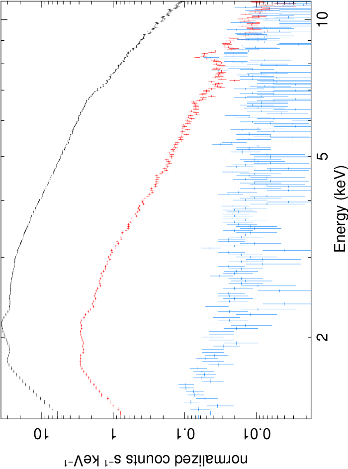
Figure 7: Source and background spectra extracted from XMM-Newton data with PN in timing mode. The background and source spectra are all rebinned using the tool pharbn (see Section 2.2.1). The black (top) spectrum is the source spectrum of XTE J1652$-$453, extracted from the RAWX columns 30 to 46; the red (middle) spectrum is the background spectrum of XTE J1652$-$453 using RAWX in [5:21]; and the blue (bottom) spectrum is the background spectrum extracted from a ‘blank-sky field’ observation of 4U 1608$-$52 using the RAWX columns 10 to 26.

As a first background correction (Model 1a) we used the background spectrum extracted from the outer parts of the CCD of the same observation of XTE J1652$-$453 (RAWX in [5:21]). This is the background spectrum contaminated with source photons. For the second background correction (Model 1b) we extracted a spectrum from a so-called blank-sky field observation that was taken with PN in timing mode, and as our last correction (Model 1c) we did not subtract any background.

Since the background can be different in different parts of the sky, for a blank-sky field we chose an observation taken in a direction close to that of XTE J1652$-$453; we therefore used the observation of the neutron-star low-mass X-ray binary 4U 1608$-$52 (obsID 0074140201) taken just after an outburst, where the source had returned to quiescence. From all the blank-sky field observations taken in a direction close to XTE J1652$-$453, the one of 4U 1608$-$52 has the most similar $N_{\rm H}$ value compared with XTE J1652$-$453. Since in the observation of 4U 1608$-$52 the source was still detectable, although it was weak, we extracted the background spectrum using the columns RAWX in [10:26], confirming that we do not include any columns contaminated with source photons. In Fig. 7 we show the background spectrum extracted from the 4U 1608$-$52 observation in blue. As can be seen from both background spectra in Fig. 7, there are emission features at $\sim 8$ keV that are due to fluorescence from the detectors and the structure surrounding them. The lines at $\sim 8$ keV are the fluorescence lines of Cu-K$\alpha$ and Zn-K$\alpha$ (see the XMM-Newton Users Handbook), and are time-dependent. Using a background spectrum from a different observation than the source spectrum, as we do for 4U 1608$-$52, may cause an incorrect background subtraction at around $\sim 7$–8 keV and may change the parameters of a possible Fe line at $\sim 7$ keV.

For the three spectral fits with different background corrections, we fit Model 1 to PN data only, covering the 1.3–10 keV range, and excluding the 1.75–2.25 keV range. As described in Section 3.3, we added an edge at $\sim 9.2$ keV. The results for the different background corrections are given in Table 2.

We set the abundances according to values reported in Anders & Grevesse (1989), and we used cross sections of Verner et al. (1996). For the purpose of comparing different background corrections, the assumed abundances and cross sections are not important. However, the best-fitting parameters and their physical interpretation can be affected when different abundance/cross-section tables are used (see following Section). For comparison, in Table 2 we also give the best-fitting results of Model 1c, where we instead used the abundances of Wilms et al. (2000) (Model 1d).

Table 2: Spectral fit results for different background corrections

Model component	Parameter	Model 1a	Model 1b	Model 1c	Model 1d
phabs	$N_{\rm H}$ ($10^{22}$)	4.75$\pm$0.03	4.66$\pm$0.04	4.64$\pm$0.03	6.78$\pm$0.03
diskbb	$kT_{\rm in}$ (keV)	0.56$\pm$0.01	0.56$\pm$0.01	0.56$\pm$0.01	0.58$\pm$0.01
	$N_{\rm dbb}$	1299${}^{+95}_{-33}$	1428${}^{+95}_{-81}$	1390${}^{+52}_{-84}$	1060${}^{+24}_{-45}$
powerlaw	$\Gamma$	2.52$\pm$0.09	2.52$\pm$0.09	2.47$\pm$0.05	2.34$\pm$0.07
	$N_{\rm\Gamma}$	0.33$\pm$0.06	0.33$\pm$0.06	0.30$\pm$0.06	0.23$\pm$0.04
Laor	$E_{\rm L}$ (keV)	6.97${}^{+0}_{-0.02}$	6.97${}^{+0}_{-0.03}$	6.97${}^{+0}_{-0.04}$	6.97${}^{+0}_{-0.02}$
	$\beta$	3.3$\pm$0.1	3.3$\pm$0.1	3.3$\pm$0.1	3.4$\pm$0.1
	$R_{\rm in}$ ($GM/c^{2}$)	4.01${}^{+0.25}_{-0.05}$	4.01${}^{+0.29}_{-0.46}$	4.01${}^{+0.23}_{-0.13}$	4.01${}^{+0.19}_{-0.07}$
	$\theta$ (deg)	6.1${}^{+3.4}_{-5.0}$	4.4${}^{+6.3}_{-4.4}$	3.5${}^{+7.0}_{-3.5}$	5.1${}^{+2.9}_{-5.1}$
	$N_{\rm L}$ ($10^{-3}$)	1.2$\pm$0.1	1.2$\pm$0.3	1.2$\pm$0.1	1.3$\pm$0.1
	EW (eV)	352${}^{+39}_{-24}$	348${}^{+73}_{-32}$	343${}^{+36}_{-29}$	375${}^{+29}_{-24}$
	$\chi^{2}_{\nu}$ ($\chi^{2}/\nu$)	1.58 (261.0/165)	1.49 (246.6/165)	1.45 (240.0/165)	1.50 (247.4/165)
	Total flux ($10^{-9}$)	8.99	9.31	9.28	8.87
NOTES.– Results are based on spectral fits to PN data of XTE J1652$-$453 in the 1.3–10 keV range. Background cor-
rections are: background of XTE J1652$-$453 contaminated with source photons (Model 1a); background of 4U 1608$-$52
(Model 1b), and no background subtracted (Model 1c & 1d).  The flux is unabsorbed and given for the 2–10 keV range,
in units of erg cm-2 s-1. Cross sections are set to Verner et al. (1996), and abundances to Anders & Grevesse (1989)
for Models 1a–c, and to Wilms et al. (2000) for Model 1d. Details about parameters are given in Section 3.3.

We find that for Models 1a–c (i.e., with abundances of Anders & Grevesse, 1989) all continuum parameters, except for $N_{\rm H}$, are consistent between the three different background corrections. The column density in Model 1a is slightly higher than in Models 1b and 1c. The diskbb normalisation is slightly lower in Model 1a than in Models 1b and 1c, but is consistent within errors. The higher $N_{\rm H}$ can be due to the over-subtraction of the background, which also explains the lower $N_{\rm dbb}$ (see also Cabanac et al., 2009, for discussion about $N_{\rm H}$ versus $N_{\rm dbb}$ relation). We conclude that for the case of XTE J1652$-$453 the choice of background correction has no effect on the continuum and line parameters. However, the issue of a contaminated background would be relevant if the diskbb normalisation is used to determine the inner disc radius.

The $\chi^{2}_{\nu}$ given in Table 2 are relatively high, although the parameters obtained from fits to only PN data are consistent with the fits to XMM-Newton/RXTE data, where the reduced $\chi^{2}$ is acceptable. The contribution to the high $\chi^{2}_{\nu}$ is most likely due to uncertainties in the detector calibration. An additional systematic error of 0.6 per cent to all PN channels is sufficient to get a $\chi^{2}_{\nu}\sim 1$.

A.2 Abundances, cross sections, and energy coverage

By investigating the effects of the different background corrections, we have used different abundances than in the rest of our analysis. By comparing the best-fitting results of Model 1d with those of Models 1a–c in Table 2, we find that the equivalent hydrogen column density is $\sim 30$ per cent lower if we used the abundances of Anders & Grevesse (1989) than if we used the abundances of Wilms et al. (2000). With the change in $N_{\rm H}$, the diskbb normalisation is significantly affected, and with this the other continuum parameters are slightly changed. Further, the best-fitting parameters of Model 1d, although slightly different, are consistent with those for Model 1 (Table 1). In other words, fitting the continuum spectrum in a relatively narrow band (1.3–10 keV, only PN) or in a wide-coverage (0.4–150 keV) did not change the parameters significantly. However, fits to only PN data resulted in larger errors on the powerlaw parameters, and also resulted in a higher powerlaw normalisation (although still consistent within errors) than for the broadband fits. With the higher powerlaw normalisation the equivalent width of the Fe emission line is clearly lower in the fits to PN data only than for the broadband fits. Nevertheless, for the case of XTE J1652$-$453 we found that even for the different continuum parameters, the Fe line parameters are not affected significantly. The best-fitting line parameters are consistent for the different background corrections, abundances, and energy coverage that we used.

References

- Anders & Grevesse (1989) Anders E., Grevesse N., 1989, Geochim. Cosmochim. Acta, 53, 197
- Arnaud (1996) Arnaud K. A., 1996, in G. H. Jacoby & J. Barnes ed., Astronomical Data Analysis Software and Systems V Vol. 101 of Astronomical Society of the Pacific Conference Series, XSPEC: The First Ten Years. p. 17
- Bardeen et al. (1972) Bardeen J. M., Press W. H., Teukolsky S. A., 1972, ApJ, 178, 347
- Belloni et al. (2005) Belloni T., Homan J., Casella P., van der Klis M., Nespoli E., Lewin W. H. G., Miller J. M., Méndez M., 2005, A&A, 440, 207
- Belloni et al. (2002) Belloni T., Psaltis D., van der Klis M., 2002, ApJ, 572, 392
- Belloni (2010) Belloni T. M., 2010, in T. Belloni ed., Lecture Notes in Physics, Berlin Springer Verlag Vol. 794 of Lecture Notes in Physics, Berlin Springer Verlag, States and Transitions in Black Hole Binaries. p. 53
- Boirin et al. (2005) Boirin L., Méndez M., Díaz Trigo M., Parmar A. N., Kaastra J. S., 2005, A&A, 436, 195
- Brenneman & Reynolds (2006) Brenneman L. W., Reynolds C. S., 2006, ApJ, 652, 1028
- Cabanac et al. (2009) Cabanac C., Fender R. P., Dunn R. J. H., Körding E. G., 2009, MNRAS, 396, 1415
- Calvelo et al. (2009) Calvelo D. E., Tzioumis T., Corbel S., Brocksopp C., Fender R. P., 2009, The Astronomer’s Telegram, 2135
- Coriat et al. (2009) Coriat M., Rodriguez J., Corbel S., Tomsick J. A., 2009, The Astronomer’s Telegram, 2219
- Czerny et al. (1991) Czerny B., Zbyszewska M., Raine D. J., 1991, in A. Treves, G. C. Perola, & L. Stella ed., Iron Line Diagnostics in X-ray Sources Vol. 385 of Lecture Notes in Physics, Berlin Springer Verlag, Compton Broadening of the Iron Line in NGC 3227. p. 226
- Done & Díaz Trigo (2009) Done C., Díaz Trigo M., 2009, ArXiv e-prints
- Done & Gierliński (2006) Done C., Gierliński M., 2006, MNRAS, 367, 659
- Done et al. (2007) Done C., Gierliński M., Kubota A., 2007, A&A Rev., 15, 1
- Dovčiak et al. (2004) Dovčiak M., Karas V., Yaqoob T., 2004, ApJS, 153, 205
- Fabian et al. (1989) Fabian A. C., Rees M. J., Stella L., White N. E., 1989, MNRAS, 238, 729
- Fabian et al. (2009) Fabian A. C., Zoghbi A., Ross R. R., Uttley P., Gallo L. C., Brandt W. N., Blustin A. J., Boller T., Caballero-Garcia M. D., Larsson J., Miller J. M., Miniutti G., Ponti G., Reis R. C., Reynolds C. S., Tanaka Y., Young A. J., 2009, Nature, 459, 540
- Gilfanov (2010) Gilfanov M., 2010, in T. Belloni ed., Lecture Notes in Physics, Berlin Springer Verlag Vol. 794 of Lecture Notes in Physics, Berlin Springer Verlag, X-Ray Emission from Black-Hole Binaries. p. 17
- Hiemstra et al. (2009) Hiemstra B., Soleri P., Méndez M., Belloni T., Mostafa R., Wijnands R., 2009, MNRAS, 394, 2080
- Homan & Belloni (2005) Homan J., Belloni T., 2005, Ap&SS, 300, 107
- Jahoda et al. (2006) Jahoda K., Markwardt C. B., Radeva Y., Rots A. H., Stark M. J., Swank J. H., Strohmayer T. E., Zhang W., 2006, ApJS, 163, 401
- Kallman & White (1989) Kallman T., White N. E., 1989, ApJ, 341, 955
- Klein-Wolt & van der Klis (2008) Klein-Wolt M., van der Klis M., 2008, ApJ, 675, 1407
- Kubota et al. (2007) Kubota A., Dotani T., Cottam J., Kotani T., Done C., Ueda Y., Fabian A. C., Yasuda T., Takahashi H., Fukazawa Y., Yamaoka K., Makishima K., Yamada S., Kohmura T., Angelini L., 2007, PASJ, 59, 185
- Laor (1991) Laor A., 1991, ApJ, 376, 90
- Lasota (2001) Lasota J., 2001, New Astronomy Review, 45, 449
- Liu et al. (2006) Liu B. F., Meyer F., Meyer-Hofmeister E., 2006, A&A, 454, L9
- Maccarone (2003) Maccarone T. J., 2003, A&A, 409, 697
- Markwardt et al. (2009) Markwardt C. B., Beardmore A. P., Miller J., Swank J. H., 2009, The Astronomer’s Telegram, 2120
- Markwardt & Swank (2009) Markwardt C. B., Swank J. H., 2009, The Astronomer’s Telegram, 2108
- Markwardt et al. (2009) Markwardt C. B., Swank J. H., Krimm H. A., Pereira D., Strohmayer T. E., 2009, The Astronomer’s Telegram, 2107
- Martocchia et al. (2006) Martocchia A., Matt G., Belloni T., Feroci M., Karas V., Ponti G., 2006, A&A, 448, 677
- McClintock & Remillard (2006) McClintock J. E., Remillard R. A., 2006, Black hole binaries. pp 157–213
- Méndez & van der Klis (1997) Méndez M., van der Klis M., 1997, ApJ, 479, 926
- Meyer et al. (2000) Meyer F., Liu B. F., Meyer-Hofmeister E., 2000, A&A, 361, 175
- Miller (2007) Miller J. M., 2007, ARA&A, 45, 441
- Miller et al. (2006) Miller J. M., Raymond J., Fabian A., Steeghs D., Homan J., Reynolds C., van der Klis M., Wijnands R., 2006, Nature, 441, 953
- Miller et al. (2004) Miller J. M., Raymond J., Fabian A. C., Homan J., Nowak M. A., Wijnands R., van der Klis M., Belloni T., Tomsick J. A., Smith D. M., Charles P. A., Lewin W. H. G., 2004, ApJ, 601, 450
- Mitsuda et al. (1984) Mitsuda K., Inoue H., Koyama K., Makishima K., Matsuoka M., Ogawara Y., Suzuki K., Tanaka Y., Shibazaki N., Hirano T., 1984, PASJ, 36, 741
- Poutanen & Svensson (1996) Poutanen J., Svensson R., 1996, ApJ, 470, 249
- Pozdnyakov et al. (1983) Pozdnyakov L. A., Sobol I. M., Syunyaev R. A., 1983, Astrophysics and Space Physics Reviews, 2, 189
- Remillard & McClintock (2006) Remillard R. A., McClintock J. E., 2006, ARA&A, 44, 49
- Reynolds & Fabian (2008) Reynolds C. S., Fabian A. C., 2008, ApJ, 675, 1048
- Reynolds et al. (2009) Reynolds M., Callanan P., Nagayama T., 2009, The Astronomer’s Telegram, 2125
- Ross & Fabian (1993) Ross R. R., Fabian A. C., 1993, MNRAS, 261, 74
- Ross & Fabian (2005) Ross R. R., Fabian A. C., 2005, MNRAS, 358, 211
- Ross & Fabian (2007) Ross R. R., Fabian A. C., 2007, MNRAS, 381, 1697
- Rossi et al. (2005) Rossi S., Homan J., Miller J. M., Belloni T., 2005, MNRAS, 360, 763
- Sala et al. (2008) Sala G., Greiner J., Ajello M., Primak N., 2008, A&A, 489, 1239
- Sala et al. (2006) Sala G., Greiner J., Haberl F., Kendziorra E., Dennerl K., Freyberg M., Hasinger G., 2006, in A. Wilson ed., The X-ray Universe 2005 Vol. 604 of ESA Special Publication, XMM-Newton Observations of the Microquasars GRO J1655-40 and GRS 1915+105. p. 291
- Shakura & Sunyaev (1973) Shakura N. I., Sunyaev R. A., 1973, A&A, 24, 337
- Thorne & Price (1975) Thorne K. S., Price R. H., 1975, ApJ, 195, L101
- Titarchuk (1994) Titarchuk L., 1994, ApJ, 434, 570
- Titarchuk et al. (2009) Titarchuk L., Laurent P., Shaposhnikov N., 2009, ApJ, 700, 1831
- Tomsick et al. (2009) Tomsick J. A., Yamaoka K., Corbel S., Kaaret P., Kalemci E., Migliari S., 2009, ApJ, 707, L87
- Torres et al. (2009) Torres M. A. P., Steeghs D., Jonker P. G., McClintock J. E., Morrell N., Roth M., 2009, The Astronomer’s Telegram, 2190
- van der Klis (1989) van der Klis M., 1989, in Ögelman H., van den Heuvel E. P. J., eds, Timing Neutron Stars Fourier techniques in X-ray timing. p. 27
- van Straaten et al. (2003) van Straaten S., van der Klis M., Méndez M., 2003, ApJ, 596, 1155
- Verner et al. (1996) Verner D. A., Ferland G. J., Korista K. T., Yakovlev D. G., 1996, ApJ, 465, 487
- Wilms et al. (2000) Wilms J., Allen A., McCray R., 2000, ApJ, 542, 914
- Yamada et al. (2009) Yamada S., Makishima K., Uehara Y., Nakazawa K., Takahashi H., Dotani T., Ueda Y., Ebisawa K., Kubota A., Gandhi P., 2009, ApJ, 707, L109
- Young et al. (2005) Young A. J., Lee J. C., Fabian A. C., Reynolds C. S., Gibson R. R., Canizares C. R., 2005, ApJ, 631, 733
- Zhang et al. (1995) Zhang W., Jahoda K., Swank J. H., Morgan E. H., Giles A. B., 1995, ApJ, 449, 930