Study of scalar meson $f_{0}(980)$ from $B\to f_{0}(980)K^{*}$ Decays

Abstract

In this paper, the branching ratios and the direct CP-violating asymmetries for decays $\bar{B}^{0}\to f_{0}(980)\bar{K}^{*0}$ and $B^{-}\to f_{0}(980)K^{*-}$ by employing the perturbative QCD factorization approach are studied. In the two-quark model supposition, $f_{0}(980)$ is commonly viewed as a mixture of $s\bar{s}$ and $n\bar{n}(\equiv(u\bar{u}+d\bar{d})/\sqrt{2})$, that is $|f_{0}(980)\rangle=|s\bar{s}\rangle\cos\theta+|n\bar{n}\rangle\sin\theta$, where $\theta$ is the $f_{0}-\sigma$ mixing angle. We find that the non-factorizable $f_{0}$ emission type diagrams can give large contributions to the final results, which are consistent with the present experimental data and the upper limit in the allowed mixing angle ranges. We predict that the direct CP asymmetry ${\cal A}^{dir}_{CP}(f_{0}(980)\bar{K}^{*0})$ is small, only a few percent, which can be tested by future B factory experiments.

I Introduction

In order to uncover the mysterious structure of the scalar meson $f_{0}(980)$, intensive studies have been done since it was firstly observed in $\pi\pi$ scattering experiments Bellef0 . There is still no consensus on the essential inner structure of $f_{0}(980)$. Some people consider it as $q\bar{q}$ state nato , or $qq\bar{qq}$ four-quark state jaffe , other people think that it is not made of one simple component but might have a more complex nature such as having a $K\bar{K}$ component jwei ; baru , or mixing with glueball celenza ; stro ; close1 , or even superpositions of the two- and four-quark states.

The B decays involved in the $f_{0}(980)$ in the final states are studied by employing various factorization approaches, such as the generalization approach GMM , the QCD factorization (QCDF) approach CYf0K ; ccy ; hycheng2 , the perturbative QCD (PQCD) approach Chenf0K1 ; Chenf0K2 ; wwang ; zhangzq1 . In these calculation, the scalar meson is usually viewed as a mixture of $s\bar{s}$ and $n\bar{n}(\equiv(u\bar{u}+d\bar{d})/\sqrt{2})$, that is

$$|f_{0}(980)\rangle=|s\bar{s}\rangle\cos\theta+|n\bar{n}\rangle\sin\theta,$$ (1)

where $\theta$ is the $f_{0}-\sigma$ mixing angle. About the value of $\theta$, there are many discussions in the phenomenal and experimental analyses theta ; theta1 . But unfortunately it is difficult to find a unique mixing angle to describe $f_{0}-\sigma$ mixing.

On the experimental side, for $f_{0}(980)$ emerging as a pole of the amplitude in the S wave kami , many channels such as $B\to f_{0}(980)K$ can be obtained by fitting of Dalitz plots of the decays $B\to\pi^{+}\pi^{-}K$ and $B\to\bar{K}KK$ and so on Bellef0 ; Bellef01 ; Bellef02 ; BaBarf0 ; BaBarf01 ; BaBarf02 . Although many such decay channels that involved $f_{0}(980)$ in the final states have been measured over the years, it has yet not been possible to account for the this scalar meson inner structure , i.e. whether one deals with a two- or rather a four-quark composite, because there still lack precise and enough data. For our considered decays, the measured values arepdg08 :

$$Br(B^{-}\to f_{0}(980)K^{*-}) = (10.4\pm 2.6)\times 10^{-6},$$ (2)

$$Br(\bar{B}^{0}\to f_{0}(980)\bar{K}^{*0}) < 8.6\times 10^{-6}.$$ (3)

It is noticed that we have assumed $Br(f_{0}(980)\to\pi^{+}\pi^{-})=0.50$ to obtain the upper experimental branching ratios.

In this paper, we will study the branching ratios and the direct CP asymmetries of $\bar{B}^{0}\to f_{0}(980)\bar{K}^{*0}$ and $B^{-}\to f_{0}(980)K^{*-}$ within perturbative QCD approach based on $k_{T}$ factorization. In the following, $f_{0}(980)$ is denoted as $f_{0}$ in some places for convenience. It is organized as follows. In Sect.II, the relevant decay constants and light-cone distribution amplitudes of $B,f_{0}$ and $K^{*}$are discussed. In Sec.III, we then analysis these decay channels using the pQCD approach. The numerical results and the discussions are given in section IV. The conclusions are presented in the final part.

II decay constants and distribution amplitudes

Now we present the wave functions to be used in the integration. For the wave function of the heavy B meson, we take:

$$\Phi_{B}(x,b)=\frac{1}{\sqrt{2N_{c}}}(P/_{B}+m_{B})\gamma_{5}\phi_{B}(x,b).$$ (4)

Here only the contribution of the Lorentz structure $\phi_{B}(x,b)$ is taken into account, since the contribution of the second Lorentz structure $\bar{\phi}_{B}$ is numerically small cdlu and has been neglected. For the distribution amplitude $\phi_{B}(x,b)$ in Eq.(4), we adopt the model

$$\phi_{B}(x,b)=N_{B}x^{2}(1-x)^{2}\exp[-\frac{M^{2}_{B}x^{2}}{2\omega^{2}_{b}}-\frac{1}{2}(\omega_{b}b)^{2}],$$ (5)

where $\omega_{b}$ is a free parameter, and the value of the normalization factor is taken as $N_{B}=91.745$ for $\omega_{b}=0.4$ in numerical calculations.

In the two-quark model, the vector decay constant $f_{f_{0}}$ and the scalar decay constant $\bar{f}_{f_{0}}$ for scalar meson $f_{0}$ can be defined as:

$$\langle f_{0}(p)|\bar{q}_{2}\gamma_{\mu}q_{1}|0\rangle = f_{f_{0}}p_{\mu},$$ (6)

$$\langle f_{0}(p)|\bar{q}_{2}q_{1}|0\rangle=m_{f_{0}}\bar{f}_{f_{0}}.$$ (7)

Owing to charge conjugation invariance or the G parity conservation, the neutral scalar meson $f_{0}$ cannot be produced via the vector current, so $f_{f_{0}}=0$. Taking the mixing into account, Eq.(7) is changed to

$$\langle f_{0}^{n}|\bar{d}d|0\rangle=\langle f_{0}^{n}|\bar{u}u|0\rangle=\frac{1}{\sqrt{2}}m_{f_{0}}\tilde{f}^{n}_{f_{0}},\,\,\,\,\langle f_{0}^{n}|\bar{s}s|0\rangle=m_{f_{0}}\tilde{f}^{s}_{f_{0}}.$$ (8)

Using the QCD sum-rule method, one can find that the scale-dependent scalar decay constants $\tilde{f}_{f_{0}}^{n}$ and $\tilde{f}_{f_{0}}^{s}$ are very closeccy . So $\tilde{f}_{f_{0}}^{n}=\tilde{f}_{f_{0}}^{s}$ is assumed and we denote them as $\bar{f}_{f_{0}}$ in the following.

The light-cone distribution amplitudes (LCDAs) for the scalar meson $f_{0}$ can be written as:

$$\langle f_{0}(p)|\bar{q}_{1}(z)_{l}q_{2}(0)_{j}|0\rangle = \frac{1}{\sqrt{2N_{c}}}\int^{1}_{0}dx\;e^{ixp\cdot z}$$ (9)

$$\times\{p\!\!\!/\Phi_{f_{0}}(x)+m_{f_{0}}\Phi^{S}_{f_{0}}(x)+m_{f_{0}}(n\!\!\!/_{+}n\!\!\!/_{-}-1)\Phi^{T}_{f_{0}}(x)\}_{jl},\quad\quad$$

here $n_{+}$ and $n_{-}$ are light-like vectors: $n_{+}=(1,0,0_{T}),n_{-}=(0,1,0_{T})$, and $n_{+}$ is parallel with the moving direction of the scalar meson $f_{0}$. The normalization can be related to the decay constants:

$$\int^{1}_{0}dx\Phi_{f_{0}}(x)=\int^{1}_{0}dx\Phi^{T}_{f_{0}}(x)=0,\,\,\,\,\,\,\,\int^{1}_{0}dx\Phi^{S}_{f_{0}}(x)=\frac{\bar{f}_{f_{0}}}{2\sqrt{2N_{c}}}\;.$$ (10)

The twist-2 LCDA can be expanded in the Gegenbauer polynomials:

$$\Phi_{f_{0}}(x,\mu) = \frac{1}{2\sqrt{2N_{c}}}\bar{f}_{f_{0}}(\mu)6x(1-x)\sum_{m=1}^{\infty}B_{m}(\mu)C^{3/2}_{m}(2x-1),$$ (11)

the values for Gegenbauer moments $B_{1},B_{3}$ have been calculated in ccy as:

$$B_{1}=-0.78\pm 0.08,\quad\quad B_{3}=0.02\pm 0.07.$$ (12)

These values are taken at $\mu=1$ GeV and the even Gegenbauer moments vanish.

As for the twist-3 distribution amplitudes $\Phi_{f_{0}}^{S}$ and $\Phi_{f_{0}}^{T}$, they have not been studied in the literature, so we adopt the asymptotic form :

$$\Phi^{S}_{f_{0}} = \frac{1}{2\sqrt{2N_{c}}}\bar{f}_{f_{0}},\,\,\,\,\,\,\,\Phi_{f_{0}}^{T}=\frac{1}{2\sqrt{2N_{c}}}\bar{f}_{f_{0}}(1-2x).$$ (13)

For our considered decays, the vector meson $K^{*}$ is longitudinally polarized. The longitudinal polarized component of the wave function is given as:

$$\Phi_{K^{*}}=\frac{1}{\sqrt{2N_{c}}}\left\{\epsilon/\left[m_{K^{*}}\Phi_{K^{*}}(x)+p/_{K^{*}}\Phi_{K^{*}}^{t}(x)\right]+m_{K^{*}}\Phi^{s}_{K^{*}}(x)\right\},$$ (14)

where the first term is the leading twist wave function (twist-2), while the second and third term are sub-leading twist (twist-3) wave functions. They can be parameterized as:

$$\Phi_{K^{*}}(x) = \frac{f_{K^{*}}}{2\sqrt{2N_{c}}}6x(1-x)\left[1+a_{1K^{*}}C^{3/2}_{1}(2x-1)+a_{2K^{*}}C^{3/2}_{2}(2x-1)\right],$$ (15)

$$\Phi^{t}_{K^{*}}(x)=\frac{3f^{T}_{K^{*}}}{2\sqrt{2N_{c}}}(1-2x),\quad\Phi^{s}_{K^{*}}(x)=\frac{3f^{T}_{K^{*}}}{2\sqrt{2N_{c}}}(2x-1)^{2},$$ (16)

where the Gegenbauer moments $a_{1K^{*}}=0.03,a_{2K^{*}}=0.11$ pball and the Gegenbauer polynomials $C^{\nu}_{n}(t)$ are given as:

$$C^{3/2}_{1}(t) = 3t,\qquad C^{3/2}_{2}(t)=\frac{3}{2}(5t^{2}-1),$$ (17)

$$C^{3/2}_{3}(t) = \frac{5}{2}t(7t^{2}-3).$$ (18)

III the perturbative QCD calculation

Under the two-quark model for the scalar meson $f_{0}$ supposition, we would like to use pQCD approach to study B decays into $f_{0}$ and $K^{*}$. The decay amplitude can be conceptually written as the convolution,

$${\cal A}(B\to f_{0}K^{*})\sim\int\!\!d^{4}k_{1}d^{4}k_{2}d^{4}k_{3}\ \mathrm{Tr}\left[C(t)\Phi_{B}(k_{1})\Phi_{f_{0}}(k_{2})\Phi_{K^{*}}(k_{3})H(k_{1},k_{2},k_{3},t)\right],$$ (19)

where $k_{i}$’s are momenta of anti-quarks included in each mesons, and $\mathrm{Tr}$ denotes the trace over Dirac and color indices. $C(t)$ is the Wilson coefficient, which results from the radiative corrections at short distance. In the above convolution, $C(t)$ includes the harder dynamics at larger scale than $M_{B}$ scale and describes the evolution of local four-Fermi operators from $m_{W}$ (the $W$ boson mass) down to $t\sim\mathcal{O}(\sqrt{\bar{\Lambda}M_{B}})$ scale, where $\bar{\Lambda}\equiv M_{B}-m_{b}$. The function $H(k_{1},k_{2},k_{3},t)$ describes the four-quark operator and the spectator quark connected by a hard gluon whose $q^{2}$ is in the order of $\bar{\Lambda}M_{B}$, and includes the $\mathcal{O}(\sqrt{\bar{\Lambda}M_{B}})$ hard dynamics. Therefore, this hard part $H$ can be perturbatively calculated.

Since the b quark is rather heavy we consider the $B$ meson at rest for simplicity. It is convenient to use light-cone coordinates $(p^{+},p^{-},{\bf p}_{T})$ to describe the meson’s momenta by

$$p^{\pm}=\frac{1}{\sqrt{2}}(p^{0}\pm p^{3}),\quad{\rm and}\quad{\bf p}_{T}=(p^{1},p^{2}).$$ (20)

Using these coordinates the $B$ meson and the two final state meson momenta can be written as

$$P_{B}=\frac{m_{B}}{\sqrt{2}}(1,1,{\bf 0}_{T}),\quad P_{2}=\frac{m_{B}}{\sqrt{2}}(1-r^{2}_{K^{*}},r^{2}_{f_{0}},{\bf 0}_{T}),\quad P_{3}=\frac{m_{B}}{\sqrt{2}}(r^{2}_{K^{*}},1-r^{2}_{f_{0}},{\bf 0}_{T}),$$ (21)

respectively. Here we have the mass ratios

$$r_{K^{*}}=m_{K^{*}}/m_{B},\quad\quad\quad r_{f_{0}}=m_{f_{0}}/m_{B}.$$ (22)

Putting the anti-quark momenta in $B$, $f_{0}$, $K^{*}$ mesons as $k_{1}$, $k_{2}$, and $k_{3}$, respectively, we can choose

$$k_{1}=(x_{1}P_{1}^{+},0,{\bf k}_{1T}),\quad k_{2}=(x_{2}P_{2}^{+},0,{\bf k}_{2T}),\quad k_{3}=(0,x_{3}P_{3}^{-},{\bf k}_{3T}).$$ (23)

For these considered decay channels, the integration over $k_{1}^{-}$, $k_{2}^{-}$, and $k_{3}^{+}$ in eq.(19) will lead to

$${\cal A}(B\to f_{0}K^{*}) \sim \int\!\!dx_{1}dx_{2}dx_{3}b_{1}db_{1}b_{2}db_{2}b_{3}db_{3}$$ (24)

$$\cdot\mathrm{Tr}\left[C(t)\Phi_{B}(x_{1},b_{1})\Phi_{f_{0}}(x_{2},b_{2})\Phi_{K^{*}}(x_{3},b_{3})H(x_{i},b_{i},t)S_{t}(x_{i})\,e^{-S(t)}\right],\quad$$

where $b_{i}$ is the conjugate space coordinate of $k_{iT}$, and $t$ is the largest energy scale in function $H(x_{i},b_{i},t)$. In order to smear the end-point singularity on $x_{i}$, the jet function $S_{t}(x)$ li02 , which comes from the resummation of the double logarithms $\ln^{2}x_{i}$, is used. The last term $e^{-S(t)}$ in Eq.(24) is the Sudakov form factor, which suppresses the soft dynamics effectively soft .

For the considered decays, the related weak effective Hamiltonian $H_{eff}$ can be written as buras96

$${\cal H}_{eff}=\frac{G_{F}}{\sqrt{2}}\,\sum_{q=u,c}V_{qb}V_{qs}^{*}\left[\left(C_{1}(\mu)O_{1}^{q}(\mu)+C_{2}(\mu)O_{2}^{q}(\mu)\right)\sum_{i=3}^{10}C_{i}(\mu)\,O_{i}(\mu)\right]\;,$$ (25)

with the Fermi constant $G_{F_{0}}=1.16639\times 10^{-5}GeV^{-2}$, and the CKM matrix elements V. We specify below the operators in ${\cal H}_{eff}$ for $b\to s$ transition:

$$\begin{array}[]{llllll}O_{1}^{u}&=&\bar{s}_{\alpha}\gamma^{\mu}Lu_{\beta}\cdot\bar{u}_{\beta}\gamma_{\mu}Lb_{\alpha}\ ,&O_{2}^{u}&=&\bar{s}_{\alpha}\gamma^{\mu}Lu_{\alpha}\cdot\bar{u}_{\beta}\gamma_{\mu}Lb_{\beta}\ ,\\ O_{3}&=&\bar{s}_{\alpha}\gamma^{\mu}Lb_{\alpha}\cdot\sum_{q^{\prime}}\bar{q}_{\beta}^{\prime}\gamma_{\mu}Lq_{\beta}^{\prime}\ ,&O_{4}&=&\bar{s}_{\alpha}\gamma^{\mu}Lb_{\beta}\cdot\sum_{q^{\prime}}\bar{q}_{\beta}^{\prime}\gamma_{\mu}Lq_{\alpha}^{\prime}\ ,\\ O_{5}&=&\bar{s}_{\alpha}\gamma^{\mu}Lb_{\alpha}\cdot\sum_{q^{\prime}}\bar{q}_{\beta}^{\prime}\gamma_{\mu}Rq_{\beta}^{\prime}\ ,&O_{6}&=&\bar{s}_{\alpha}\gamma^{\mu}Lb_{\beta}\cdot\sum_{q^{\prime}}\bar{q}_{\beta}^{\prime}\gamma_{\mu}Rq_{\alpha}^{\prime}\ ,\\ O_{7}&=&\frac{3}{2}\bar{s}_{\alpha}\gamma^{\mu}Lb_{\alpha}\cdot\sum_{q^{\prime}}e_{q^{\prime}}\bar{q}_{\beta}^{\prime}\gamma_{\mu}Rq_{\beta}^{\prime}\ ,&O_{8}&=&\frac{3}{2}\bar{s}_{\alpha}\gamma^{\mu}Lb_{\beta}\cdot\sum_{q^{\prime}}e_{q^{\prime}}\bar{q}_{\beta}^{\prime}\gamma_{\mu}Rq_{\alpha}^{\prime}\ ,\\ O_{9}&=&\frac{3}{2}\bar{s}_{\alpha}\gamma^{\mu}Lb_{\alpha}\cdot\sum_{q^{\prime}}e_{q^{\prime}}\bar{q}_{\beta}^{\prime}\gamma_{\mu}Lq_{\beta}^{\prime}\ ,&O_{10}&=&\frac{3}{2}\bar{s}_{\alpha}\gamma^{\mu}Lb_{\beta}\cdot\sum_{q^{\prime}}e_{q^{\prime}}\bar{q}_{\beta}^{\prime}\gamma_{\mu}Lq_{\alpha}^{\prime}\ ,\end{array}$$ (31)

where $\alpha$ and $\beta$ are the $SU(3)$ color indices; $L$ and $R$ are the left- and right-handed projection operators with $L=(1-\gamma_{5})$, $R=(1+\gamma_{5})$. The sum over $q^{\prime}$ runs over the quark fields that are active at the scale $\mu=O(m_{b})$, i.e., $(q^{\prime}\epsilon\{u,d,s,c,b\})$.

In the following, we take the $\bar{B}^{0}\to f_{0}\bar{K}^{*0}$ decay channel as an example to expound. There are 8 type diagrams contributing to this decay, as illustrated in Fig.1. For the factorizable emission diagrams (a) and (b), operators $O_{1-4,9,10}$ are $(V-A)(V-A)$ currents, and the operators $O_{5-8}$ have the structure of $(V-A)(V+A)$, the sum of the their amplitudes are written as $F_{eK^{*}}$ and $F_{eK^{*}}^{P1}$, respectively. For $\langle f_{0}|\bar{q}\gamma_{\mu}q|0\rangle=0$, one then finds that

$$F_{eK^{*}} = F_{eK^{*}}^{P1}=0.$$ (32)

In order to get the right flavor and color structure for factorization to work, a Fierz transformation for the $(V-A)(V+A)$ operators may sometimes be needed and then the corresponding amplitude is

Figure 1: Diagrams contributing to the decay $\bar{B}^{0}\to f_{0}(980)\bar{K}^{*0}$ .

$$F^{P2}_{eK^{*}} = -16\pi C_{F}m_{B}^{4}r_{f_{0}}{\bar{f}_{f_{0}}}\int_{0}^{1}dx_{1}dx_{3}\int_{0}^{\infty}b_{1}db_{1}\,b_{3}db_{3}\,\Phi_{B}(x_{1},b_{1})$$ (33)

$$\times\bigg{\{}\left[\Phi_{K^{*}}(x_{3})-r_{K^{*}}x_{3}\left(\Phi_{K^{*}}^{s}(x_{3})+\Phi_{K^{*}}^{t}(x_{3})\right)-2r_{K^{*}}\Phi_{K^{*}}^{s}(x_{3})\right]$$

$$\;\;\;\;\times E_{ei}(t)h_{e}(x_{1},x_{3},b_{1},b_{3})-2r_{K^{*}}\Phi_{K^{*}}^{s}(x_{3})E_{ei}(t^{\prime})h_{e}(x_{3},x_{1},b_{3},b_{1})\bigg{\}}\;,$$

where $C_{F}=4/3$ is the group factor of the $SU(3)_{c}$ gauge group. The functions $E_{ei}(t^{(\prime)})$ and $h_{e}$ including the Sudakov factor and jet function have the same definition as those in Ref. wwang ; zhangzq1 .

For the non-factorizable diagrams 1(c) and 1(d), all three meson wave functions are involved. The integration of $b_{3}$ can be performed using the $\delta$ function $\delta(b_{3}-b_{2})$, leaving only integration of $b_{1}$ and $b_{2}$. For the $(V-A)(V-A)$, $(V-A)(V+A)$, $(S-P)(S+P)$ operators, the results are

$${\cal M}_{eK^{*}} = 32\pi C_{F}m_{B}^{4}/\sqrt{2N_{C}}\int_{0}^{1}dx_{1}dx_{2}dx_{3}\int_{0}^{\infty}b_{1}db_{1}\,b_{2}db_{2}\,\Phi_{B}(x_{1},b_{1})\Phi_{f_{0}}(x_{2})$$ (34)

$$\bigg{\{}[(x_{2}-1)\Phi_{K^{*}}(x_{3})-r_{K^{*}}x_{3}(\Phi_{K^{*}}^{s}(x_{3})+\Phi_{K^{*}}^{t}(x_{3}))]E^{\prime}_{ei}(t)h_{n}(x_{1},1-x_{2},x_{3},b_{1},b_{2})$$

$$+[(x_{2}+x_{3})\Phi_{K^{*}}(x_{3})+r_{K^{*}}x_{3}\left(\Phi_{K^{*}}^{s}(x_{3})-\Phi_{K^{*}}^{t}(x_{3})\right]E^{\prime}_{ei}(t^{\prime})h_{n}(x_{1},x_{2},x_{3},b_{1},b_{2})\bigg{\}},\;\;\;\quad$$

$${\cal M}^{P1}_{eK^{*}} = 32\pi C_{F}m_{B}^{4}r_{f_{0}}/\sqrt{2N_{C}}\int_{0}^{1}dx_{1}dx_{2}dx_{3}\int_{0}^{\infty}b_{1}db_{1}\,b_{2}db_{2}\,\Phi_{B}(x_{1},b_{1})$$ (35)

$$\times\bigg{\{}E^{\prime}_{ei}(t)h_{n}(x_{1},1-x_{2},x_{3},b_{1},b_{2})\left[(x_{2}-1)\Phi_{K^{*}}(x_{3})\left(\Phi_{f_{0}}^{S}(x_{2})-\Phi_{f_{0}}^{T}(x_{2})\right)\right.$$

$$\;\;\;\;\;\;-r_{K^{*}}(x_{2}-1)\left(\Phi_{K^{*}}^{s}(x_{3})+\Phi_{K^{*}}^{t}(x_{3})\right)\left(\Phi_{f_{0}}^{S}(x_{2})-\Phi_{f_{0}}^{T}(x_{2})\right)$$

$$\;\;\;\;\;\;\left.+r_{K^{*}}x_{3}\left(\Phi_{K^{*}}^{s}(x_{3})-\Phi_{K^{*}}^{t}(x_{3})\right)\left(\Phi_{f_{0}}^{S}(x_{2})+\Phi_{f_{0}}^{T}(x_{2})\right)\right]$$

$$\;\;\;\;\;\;+E^{\prime}_{ei}(t^{\prime})h_{n}(x_{1},x_{2},x_{3},b_{1},b_{2})\left[x_{2}\Phi_{K^{*}}(x_{3})\left(\Phi_{f_{0}}^{S}(x_{2})+\Phi_{f_{0}}^{T}(x_{2})\right)\right.$$

$$\;\;\;\;\;-r_{K^{*}}x_{2}\left(\Phi_{K^{*}}^{s}(x_{3})+\Phi_{K^{*}}^{t}(x_{3})\right)\left(\Phi_{f_{0}}^{S}(x_{2})+\Phi_{f_{0}}^{T}(x_{2})\right)$$

$$\;\;\;\;\;\;\left.-r_{K^{*}}x_{3}\left(\Phi_{K^{*}}^{s}(x_{3})-\Phi_{K^{*}}^{t}(x_{3})\right)\left(\Phi_{f_{0}}^{S}(x_{2})-\Phi_{f_{0}}^{T}(x_{2})\right)\right]\bigg{\}}\;,$$

$${\cal M}^{P2}_{eK^{*}} = -32\pi C_{F}m_{B}^{4}/\sqrt{2N_{C}}\int_{0}^{1}dx_{1}dx_{2}dx_{3}\int_{0}^{\infty}b_{1}db_{1}\,b_{2}db_{2}\,\Phi_{B}(x_{1},b_{1})\Phi_{f_{0}}(x_{2})$$ (36)

$$\times\bigg{\{}\left[(-x_{2}+x_{3}+1)\Phi_{K^{*}}(x_{3})+r_{K^{*}}x_{3}\left(\Phi_{K^{*}}^{s}(x_{3})-\Phi_{K^{*}}^{t}(x_{3})\right)\right]$$

$$\times E^{\prime}_{ei}(t)h_{n}(x_{1},1-x_{2},x_{3},b_{1},b_{2})-E^{\prime}_{ei}(t^{\prime})h_{n}(x_{1},x_{2},x_{3},b_{1},b_{2})$$

$$\times\left[x_{2}\Phi_{K^{*}}(x_{3})+r_{K^{*}}x_{3}(\Phi_{K^{*}}^{s}(x_{3})+\Phi_{K^{*}}^{t}(x_{3}))\right]\bigg{\}}\;.$$

For the non-factorizable annihilation diagrams (e) and (f), again all three wave functions are involved. $M_{aK^{*}}$, $M_{aK^{*}}^{P1}$ and $M_{aK^{*}}^{P2}$ describe the contributions from the $(V-A)(V-A)$, $(V-A)(V+A)$ and $(S-P)(S+P)$ type operators, respectively,

$${\cal M}_{aK^{*}} = 32\pi C_{F}m_{B}^{4}/\sqrt{2N_{C}}\int_{0}^{1}dx_{1}dx_{2}dx_{3}\int_{0}^{\infty}b_{1}db_{1}\,b_{2}db_{2}\,\Phi_{B}(x_{1},b_{1})\left\{\left[x_{2}\Phi_{K^{*}}(x_{3})\Phi_{f_{0}}(x_{2})\right.\right.$$ (37)

$$\left.\left.+r_{K^{*}}r_{f_{0}}\Phi_{f_{0}}^{T}(x_{2})\left((x_{2}+x_{3}-1)\Phi_{K^{*}}^{s}(x_{3})+(x_{2}-x_{3}-1)\Phi_{K^{*}}^{t}(x_{3})\right)\right.\right.$$

$$\left.\left.-r_{K^{*}}r_{f_{0}}\Phi_{f_{0}}^{S}(x_{2})\left((x_{2}-x_{3}+3)\Phi_{K^{*}}^{s}(x_{3})+(x_{2}+x_{3}-1)\Phi_{K^{*}}^{t}(x_{3})\right)\right]E^{\prime}_{ai}(t)\right.$$

$$\left.\times h_{na}(x_{1},x_{2},x_{3},b_{1},b_{2})+E^{\prime}_{ai}(t^{\prime})h^{\prime}_{na}(x_{1},x_{2},x_{3},b_{1},b_{2})\left[(x_{3}-1)\Phi_{K^{*}}(x_{3})\Phi_{f_{0}}(x_{2})\right.\right.$$

$$\left.\left.+r_{K^{*}}r_{f_{0}}\Phi_{f_{0}}^{S}(x_{2})\left((x_{2}-x_{3}+1)\Phi_{K^{*}}^{s}(x_{3})-(x_{2}+x_{3}-1)\Phi_{K^{*}}^{t}(x_{3})\right)\right.\right.$$

$$\left.\left.-r_{K^{*}}r_{f_{0}}\Phi_{f_{0}}^{T}(x_{2})\left((1-x_{2}-x_{3})\Phi_{K^{*}}^{s}(x_{3})+(1+x_{2}-x_{3})\Phi_{K^{*}}^{t}(x_{2})\right)\right]\right\}\;,$$

$${\cal M}^{P1}_{aK^{*}} = 32\pi C_{F}m_{B}^{4}/\sqrt{2N_{C}}\int_{0}^{1}dx_{1}dx_{2}dx_{3}\int_{0}^{\infty}b_{1}db_{1}\,b_{2}db_{2}\,\Phi_{B}(x_{1},b_{1})$$ (38)

$$\times\bigg{\{}\left[r_{K^{*}}(1+x_{3})\Phi_{f_{0}}(x_{2})(\Phi_{K^{*}}^{t}(x_{3})+\Phi_{K^{*}}^{s}(x_{3}))-r_{f_{0}}(x_{2}-2)\Phi_{K^{*}}(x_{3})\left(\Phi_{f_{0}}^{S}(x_{2})\right.\right.$$

$$\;\;\left.\left.-\Phi_{f_{0}}^{T}(x_{2})\right)\right]E^{\prime}_{ai}(t)h_{na}(x_{1},x_{2},x_{3},b_{1},b_{2})-E^{\prime}_{ai}(t^{\prime})h^{\prime}_{na}(x_{1},x_{2},x_{3},b_{1},b_{2})\left[r_{K^{*}}\right.$$

$$\left.\times(x_{3}-1)\Phi_{f_{0}}(x_{2})(\Phi_{K^{*}}^{t}(x_{3})+\Phi_{K^{*}}^{s}(x_{3}))-r_{f_{0}}x_{2}\Phi_{K^{*}}(x_{3})(\Phi_{f_{0}}^{S}(x_{2})-\Phi_{f_{0}}^{T}(x_{2}))\right]\bigg{\}},\;\;\;\;\;\;$$

$${\cal M}^{P2}_{aK^{*}} = 32\pi C_{F}m_{B}^{4}/\sqrt{2N_{C}}\int_{0}^{1}dx_{1}dx_{2}dx_{3}\int_{0}^{\infty}b_{1}db_{1}\,b_{2}db_{2}\,\Phi_{B}(x_{1},b_{1})$$ (39)

$$\times\bigg{\{}\left[(x_{3}-1)\Phi_{f_{0}}(x_{2})\right.\Phi_{K^{*}}(x_{3})+4r_{K^{*}}r_{f_{0}}\Phi^{S}_{f_{0}}(x_{2})\Phi_{K^{*}}^{s}(x_{3})+r_{K^{*}}r_{f_{0}}\left((x_{2}-x_{3}-1)\right.$$

$$\;\times\left(\Phi_{K^{*}}^{s}(x_{3})\Phi_{f_{0}}^{S}(x_{2})-\Phi_{K^{*}}^{t}(x_{3})\Phi_{f_{0}}^{T}(x_{2})\right.)\left.+(x_{2}+x_{3}-1)\left(\Phi_{K^{*}}^{s}(x_{3})\Phi_{f_{0}}^{T}(x_{2})\right.\right.$$

$$\left.\left.-\Phi_{K^{*}}^{t}(x_{3})\Phi_{f_{0}}^{S}(x_{2})\right)\right]E^{\prime}_{ai}(t)h_{na}(x_{1},x_{2},x_{3},b_{1},b_{2})+E^{\prime}_{ai}(t^{\prime})h^{\prime}_{na}(x_{1},x_{2},x_{3},b_{1},b_{2})$$

$$\;\;\times\left[x_{2}\Phi_{f_{0}}(x_{2})\Phi_{K^{*}}(x_{3})-x_{2}r_{K^{*}}r_{f_{0}}(\Phi_{f_{0}}^{S}(x_{2})-\Phi_{f_{0}}^{T}(x_{2}))(\Phi_{K^{*}}^{s}(x_{3})+\Phi_{K^{*}}^{t}(x_{3}))\right.$$

$$\;\;\;\left.-r_{K^{*}}r_{f_{0}}(1-x_{3})(\Phi_{f_{0}}^{S}(x_{2})+\Phi_{f_{0}}^{T}(x_{2}))(\Phi_{K^{*}}^{s}(x_{3})-\Phi_{K^{*}}^{t}(x_{3}))\right]\bigg{\}}\;.$$

The factorizable annihilation diagrams (g) and (h) involve only two final state mesons’ wave functions. There are also three kinds of decay amplitudes for these two diagrams. $F_{aK^{*}}$ is for $(V-A)(V-A)$ type operators, $F_{aK^{*}}^{P1}$ is for $(V-A)(V+A)$ type operators, while $F_{aK^{*}}^{P2}$ is for $(S-P)(S+P)$ type operators:

$$F_{aK^{*}} = F^{P1}_{aK^{*}}=-8\pi C_{F}m_{B}^{4}f_{B}\int_{0}^{1}dx_{2}dx_{3}\int_{0}^{\infty}b_{2}db_{2}\,b_{3}db_{3}\left\{\left[(x_{3}-1)\Phi_{K^{*}}(x_{3})\Phi_{f_{0}}(x_{2})\right.\right.$$ (40)

$$\left.\left.-2r_{K^{*}}r_{f_{0}}(x_{3}-2)\Phi_{K^{*}}^{s}(x_{3})\Phi_{f_{0}}^{S}(x_{2})-2r_{K^{*}}r_{f_{0}}x_{3}\Phi_{K^{*}}^{t}(x_{3})\Phi_{f_{0}}^{S}(x_{2})\right]\right.$$

$$\left.\times E_{ai}(t)h_{a}(x_{2},1-x_{3},b_{2},b_{3})+E_{ai}(t^{\prime})h_{a}(1-x_{3},x_{2},b_{3},b_{2})\right.$$

$$\left.\times[x_{2}\Phi_{K^{*}}(x_{3})\Phi_{f_{0}}(x_{2})-2r_{K^{*}}r_{f_{0}}\Phi_{K^{*}}^{s}(x_{3})((x_{2}+1)\Phi_{f_{0}}^{S}(x_{2})-(x_{2}-1)\Phi_{f_{0}}^{T})]\right\},$$

$$F^{P2}_{aK^{*}} = 16\pi C_{F}m_{B}^{4}f_{B}\int_{0}^{1}dx_{2}dx_{3}\int_{0}^{\infty}b_{2}db_{2}\,b_{3}db_{3}$$ (41)

$$\times\bigg{\{}[r_{K^{*}}(x_{3}-1)\Phi_{f_{0}}(x_{2})(\Phi_{K^{*}}^{s}(x_{3})-\Phi_{K^{*}}^{t}(x_{3}))+2r_{f_{0}}\Phi_{K^{*}}(x_{3})\Phi_{f_{0}}^{S}(x_{2})]$$

$$\times E_{ai}(t)h_{a}(x_{2},1-x_{3},b_{2},b_{3})-E_{ai}(t^{\prime})h_{a}(1-x_{3},x_{2},b_{3},b_{2})$$

$$\times[2r_{K^{*}}\Phi_{K^{*}}^{s}(x_{3})\Phi_{f_{0}}(x_{2})-r_{f_{0}}x_{2}\Phi_{K^{*}}(x_{3})(\Phi_{f_{0}}^{T}(x_{2})+\Phi_{f_{0}}^{S}(x_{2}))]\bigg{\}}.$$

If we exchange the $K^{*}$ and $f_{0}$ in Fig.1, the corresponding expressions of amplitudes for new diagrams will be similar with those as given in Eqs.(34-41) and can be obtained by the replacements:

$$\Phi_{f_{0}}(x)\longleftrightarrow\Phi_{K^{*}}(x),\Phi^{S}_{f_{0}}(x)\longleftrightarrow\Phi^{s}_{K^{*}}(x),\Phi^{T}_{f_{0}}(x)\longleftrightarrow\Phi^{t}_{K^{*}}(x),r_{f_{0}}\longleftrightarrow r_{K^{*}},$$ (42)

since the wave functions for the mesons $f_{0}(980)$ and $K^{*}$ have exactly the same form. The only difference is some normalization constants for the different twist distribution amplitudes. That is, the factorization formulae for (a) and (b) in the new diagrams amplitudes are written as:

$$F_{ef_{0}} = -8\pi C_{F}m_{B}^{4}f_{K^{*}}\int_{0}^{1}dx_{1}dx_{2}\int_{0}^{\infty}b_{1}db_{1}\,b_{2}db_{2}\,\Phi_{B}(x_{1},b_{1})$$ (43)

$$\times\bigg{\{}\left[(1+x_{2})\Phi_{f_{0}}(x_{2})-r_{f_{0}}(1-2x_{2})\left(\Phi_{f_{0}}^{S}(x_{2})-\Phi_{f_{0}}^{T}(x_{2})\right)\right]E_{ei}(t)h_{e}(x_{1},x_{2},b_{1},b_{2})$$

$$\;\;\;\;\;\;-2r_{f_{0}}\Phi_{f_{0}}^{S}({x_{2}})E_{ei}(t^{\prime})h_{e}(x_{2},x_{1},b_{2},b_{1})\bigg{\}}\;,$$

$$F^{P2}_{ef_{0}} = 0.$$ (44)

Since we have chosen the momentum fraction at the anti-quark, we should use $\Phi^{(S,T)}_{f_{0}}(1-x)$ and $\Phi^{(s,t)}_{K^{*}}(1-x)$ for the mesons $f_{0}(980)$ and $K^{*}$ in the calculation. But for simplicity, we use $\Phi^{(S,T)}_{f_{0}}(x)$ and $\Phi^{(s,t)}_{K^{*}}(x)$ to denote $\Phi^{(S,T)}_{f_{0}}(1-x)$ and $\Phi^{(s,t)}_{K^{*}}(1-x)$ in the upper formulae.

Combining the contributions from different diagrams, the total decay amplitudes for the decays $\bar{B}^{0}\to f_{0}\bar{K}^{*0}$ and $B^{-}\to f_{0}K^{*-}$ can be written as:

$${\cal M}(f_{0}K^{0}) = \xi_{u}M_{eK^{*}}C_{2}F_{1}(\theta)-\xi_{t}\left\{F_{ef_{0}}(a_{4}-\frac{a_{10}}{2})F_{1}(\theta)+[F^{P2}_{ef_{0}}F_{1}(\theta)+F^{P2}_{eK^{*}}F_{2}(\theta)](a_{6}-\frac{a_{8}}{2})\right.$$ (45)

$$\left.+[M_{ef_{0}}(C_{3}-\frac{C_{9}}{2})+M_{eK^{*}}(2C_{4}+\frac{C_{10}}{2})]F_{1}(\theta)+M_{eK^{*}}(C_{3}+C_{4}-\frac{C_{9}}{2}-\frac{C_{10}}{2})\right.$$

$$\left.\times F_{2}(\theta)+[M^{P1}_{ef_{0}}F_{1}(\theta)+M^{P1}_{eK^{*}}F_{2}(\theta)](C_{5}-\frac{C_{7}}{2})+M^{P2}_{eK^{*}}\left[(2C_{6}+\frac{C_{8}}{2})F_{1}(\theta)\right.\right.$$

$$\left.\left.+(C_{6}-\frac{C_{8}}{2})F_{2}(\theta)\right]+\left[M_{af_{0}}F_{1}(\theta)+M_{aK^{*}}F_{2}(\theta)\right](C_{3}-\frac{C_{9}}{2})+\left[M^{P1}_{af_{0}}F_{1}(\theta)\right.\right.$$

$$\left.\left.+M^{P1}_{aK^{*}}F_{2}(\theta)\right](C_{5}-\frac{C_{7}}{2})+[F_{af_{0}}F_{1}(\theta)+F_{aK^{*}}F_{2}(\theta)](a_{4}-\frac{a_{10}}{2})\right.$$

$$\left.+[F^{P2}_{af_{0}}F_{1}(\theta)+F^{P2}_{aK^{*}}F_{2}(\theta)](a_{6}-\frac{a_{8}}{2})\right\},$$

$${\cal M}(f_{0}K^{*-}) = \xi_{u}[(F_{ef_{0}}a_{1}+M_{eK^{*}}C_{2}+M_{ef_{0}}C_{1}+M_{af_{0}}C_{1}+F_{af_{0}}a_{1})F_{1}(\theta)+\left(M_{aK^{*}}\right.$$ (46)

$$\left.\times C_{1}+F_{aK^{*}}a_{1}\right)F_{2}(\theta)]-\xi_{t}\left\{F_{ef_{0}}(a_{4}+a_{10})F_{1}(\theta)+F^{P2}_{ef_{0}}F_{1}(\theta)(a_{6}+a_{8})\right.$$

$$\left.+F^{P2}_{eK^{*}}F_{2}(\theta)(a_{6}-\frac{a_{8}}{2})+[M_{ef_{0}}(C_{3}+C_{9})+M_{eK^{*}}(2C_{4}+\frac{C_{10}}{2})]F_{1}(\theta)\right.$$

$$\left.+M_{eK^{*}}(C_{3}+C_{4}-\frac{C_{9}}{2}-\frac{C_{10}}{2})F_{2}(\theta)+M^{P1}_{ef_{0}}F_{1}(\theta)(C_{5}+C_{7})+M^{P1}_{eK^{*}}\right.$$

$$\left.\times F_{2}(\theta)(C_{5}-\frac{C_{7}}{2})+M^{P2}_{eK^{*}}[(2C_{6}+\frac{C_{8}}{2})F_{1}(\theta)+(C_{6}-\frac{C_{8}}{2})F_{2}(\theta)]\right.$$

$$\left.+[M_{af_{0}}F_{1}(\theta)+M_{aK^{*}}F_{2}(\theta)](C_{3}+C_{9})+[M^{P1}_{af_{0}}F_{1}(\theta)+M^{P1}_{aK^{*}}F_{2}(\theta)]\right.$$

$$\left.\times(C_{5}+C_{7})+[F_{af_{0}}F_{1}(\theta)+F_{aK^{*}}F_{2}(\theta)](a_{4}+a_{10})\right.$$

$$\left.+[F^{P2}_{af_{0}}F_{1}(\theta)+F^{P2}_{aK^{*}}F_{2}(\theta)](a_{6}+a_{8})\right\},$$

where $\xi_{u}=V_{ub}V^{*}_{us},\xi_{t}=V_{tb}V^{*}_{ts}$ and $F_{1}(\theta)=\sin\theta/\sqrt{2},F_{2}(\theta)=\cos\theta$. The combinations of the Wilson coefficients are defined as usual AKL :

$$a_{1}(\mu) = C_{2}(\mu)+\frac{C_{1}(\mu)}{3},\quad a_{2}(\mu)=C_{1}(\mu)+\frac{C_{2}(\mu)}{3},$$

$$a_{i}(\mu) = C_{i}(\mu)+\frac{C_{i+1}(\mu)}{3},\quad i=3,5,7,9,$$

$$a_{i}(\mu) = C_{i}(\mu)+\frac{C_{i-1}(\mu)}{3},\quad i=4,6,8,10.$$ (47)

IV Numerical results and discussions

Table 1: Input parameters used in the numerical calculationccy ; pdg08 .

Masses	$m_{f_{0}}=0.980\mbox{ GeV}$,	$m_{K^{*}}=0.892\mbox{ GeV}$,
	$M_{B}=5.28\mbox{ GeV}$,
Decay constants	$f_{B}=0.19\mbox{ GeV}$,	$f_{f_{0}}=0.37\mbox{ GeV}$,
	$f_{K^{*}}=0.217\mbox{ GeV}$,	$f^{T}_{K^{*}}=0.185\mbox{ GeV}$,
Lifetimes	$\tau_{B^{\pm}}=1.638\times 10^{-12}\mbox{ s}$,	$\tau_{B^{0}}=1.530\times 10^{-12}\mbox{ s}$,
$CKM$	$V_{tb}=1.0$,	$V_{ts}=-0.0387$,
	$V_{us}=0.2255$,	$V_{ub}=0.00393e^{-i60^{\circ}}$.

In the numerical calculation, we will use the input parameters as listed in Table 1.

From Eq.(43), we can find the numerical values of the corresponding form factor $F^{\bar{B}^{0}\to f_{0}(d\bar{d})}_{0}$at maximal recoiling:

$$F^{\bar{B}^{0}\to f_{0}(d\bar{d})}_{0}=0.31,$$ (48)

which is smaller than $F^{\bar{B}^{0}\to f_{0}(980)(d\bar{d})}=0.47$ wwang , for using different values for the threshold parameters $c$ in the jet function.

In the B-rest frame, the decay rate of $B\to f_{0}(980)K^{*}$ can be written as:

$$\Gamma=\frac{G_{F}^{2}}{32\pi m_{B}}|{\cal M}|^{2}(1-r^{2}_{f_{0}}-r^{2}_{K^{*}}),$$ (49)

where $r_{f_{0}},r_{K^{*}}$ have been defined in Eq.(22) and ${\cal M}$ is the total decay amplitude of $B\to f_{0}(980)K^{*}$, which has been given in section III.

Using the wave functions as specified in the previous section and the input parameters listed in Table 1, it is straightforward to calculate the CP-averaged branching ratios for the considered decays.

If $f_{0}(980)$ is purely composed of $s\bar{s}$, the branching ratios of $B\to f_{0}(980)K^{*}$ are:

$$Br(\bar{B}^{0}\to f_{0}(980)\bar{K}^{*0})=(14.0^{+1.5+1.2+2.9}_{-1.4-1.1-3.0})\times 10^{-6},$$ (50)

$$Br(B^{-}\to f_{0}(980)K^{*-})=(15.4^{+1.6+1.4+4.1}_{-1.5-1.2-4.3})\times 10^{-6},$$ (51)

where the uncertainties are from the decay constant of $f_{0}(980)$, the Gegenbauer moments $B_{1}$ and $B_{3}$. If $f_{0}(980)$ is purely composed of $n\bar{n}$, the branching ratios for $B\to f_{0}(980)K^{*}$ are:

$$Br(\bar{B}^{0}\to f_{0}(980)\bar{K}^{*0})=(2.2^{+0.3+0.4+1.2}_{-0.2-0.5-1.1})\times 10^{-6},$$ (52)

$$Br(B^{-}\to f_{0}(980)K^{*-})=(4.0^{+0.5+0.5+1.6}_{-0.4-0.7-1.7})\times 10^{-6},$$ (53)

where the uncertainties are from the same quantities as above.

The branching ratio for decay $B^{-}\to f_{0}(980)K^{*-}$ in the upper extreme case is consistent with QCDF results hycheng2 :

$$Br(B^{-}\to f_{0}(980)K^{*-})=\begin{cases}14.3\times 10^{-6},\text{for}f_{0}(980)=s\bar{s},\\ 6.9\times 10^{-6},\text{for}f_{0}(980)=n\bar{n}.\end{cases}$$ (54)

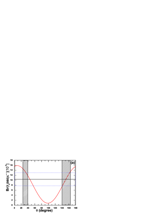
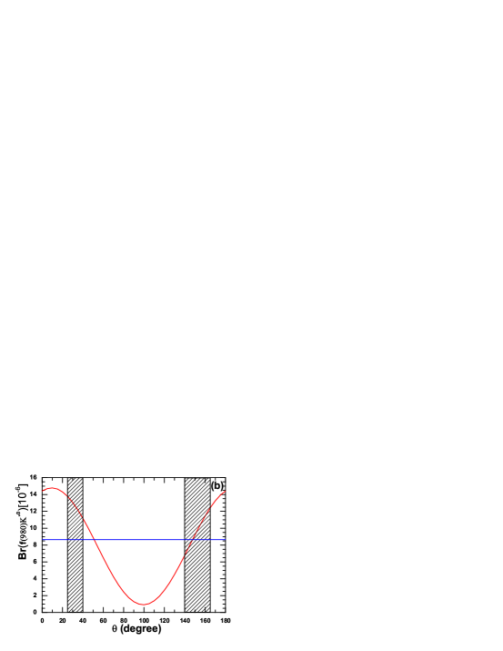
Figure 2: The $\theta$ dependence of the branching ratios (in units of $10^{-6}$) of the decays (a) $B^{-}\to f_{0}(980)K^{*-}$ and (b) $\bar{B}^{0}\to f_{0}(980)\bar{K}^{*0}$. The horizontal solid lines show (a) the measured value and (b) the experimental upper limit, respectively. The horizontal band within the doted lines shows the experimentally allowed region of decay $B^{-}\to f_{0}(980)K^{*-}$. The vertical bands show two possible ranges of $\theta$: $25^{\circ}<\theta<40^{\circ}$ and $140^{\circ}<\theta<165^{\circ}$.

The Branching ratio of $B\to f_{0}(980)K^{*}$ depends on the mixing angle $\theta$ of strange and nonstrange components of the $f_{0}(980)$. In Fig.3, we plot the branching ratios as functions of the mixing angle $\theta$. Using the above mentioned range of the mixing angle, we obtain:

$$Br(B^{-}\to f_{0}(980)K^{*-})=(11.7\sim 14.6)\times 10^{-6},$$ (55)

$$Br(\bar{B}^{0}\to f_{0}(980)\bar{K}^{*0})=(11.2\sim 13.7)\times 10^{-6},$$ (56)

for $25^{\circ}<\theta<40^{\circ}$; as for the other range $140^{\circ}<\theta<165^{\circ}$, these two branching ratios are:

$$Br(B^{-}\to f_{0}(980)K^{*-})=(7.5\sim 13.5)\times 10^{-6},$$ (57)

$$Br(\bar{B}^{0}\to f_{0}(980)\bar{K}^{*0})=(6.7\sim 12.5)\times 10^{-6},$$ (58)

where only the central values of other input parameters are used. It is easy to see that the pQCD predictions can account for the measured value or the experimental upper limit in the range $140^{\circ}<\theta<165^{\circ}$ (shown in Fig.2). From the Fig.2(b), one can find the branching ratio of $\bar{B}^{0}\to f_{0}(980)\bar{K}^{*0}$ should be not far away from the upper limit (i.e. $8.6\times 10^{-6}$). If we take $\theta=140^{\circ}$, the value of $Br(\bar{B}^{0}\to f_{0}(980)\bar{K}^{*0})$ is about $6.8\times 10^{-6}$, which is consistent with the experimental value, $(5.2\pm 2.2)\times 10^{-6}$ aubert . But for $25^{\circ}<\theta<40^{\circ}$, the predicted $\bar{B}^{0}\to f_{0}(980)\bar{K}^{*0}$ rate exceeds the current experimental limit.

Table 2: Decay amplitudes for $\bar{B}^{0}\to f_{0}(980)\bar{K}^{*0}$ ($\times 10^{-2}\mbox{GeV}^{3}$), where ”this work” denotes the results using the distribution amplitudes $\Phi_{f_{0}}$, $\Phi^{S}_{f_{0}}$ and $\Phi^{T}_{f_{0}}$ given in the previous section, ”Chenf0K1 ” denotes the results using the DAs proposed in Chenf0K1 .

$\bar{s}s$		$F^{f_{0}}_{e\bar{K}^{*0}}$	$M^{f_{0}}_{e\bar{K}^{*0}}$	$M^{f_{0}}_{a\bar{K}^{*0}}$	$F^{f_{0}}_{a\bar{K}^{*0}}$
This work		6.02	$1.12+4.37i$	$-0.45-0.78i$	$0.32+7.32i$
Chenf0K1		3.25	$0.29+0.31i$	$0.56-0.70i$	$-7.49+0.42i$
$\bar{n}n$		$F^{\bar{K}^{*0}}_{ef_{0}}$	$M^{f_{0},T}_{e\bar{K}^{*0}}$	$M^{f_{0}}_{e\bar{K}^{*0}}$	$M^{\bar{K}^{*0}}_{ef_{0}}$
This work		-6.74	$-19.47-59.17i$	$2.9+11.3i$	$0.81-0.56i$
Chenf0K1		10.5	$7.54+6.97i$	$0.27+0.28i$	$-0.37+1.81i$
$\bar{n}n$		$M^{\bar{K}^{*0}}_{af_{0}}$	$F^{\bar{K}^{*0}}_{af_{0}}$
This work		$0.17+0.13i$	$0.35-6.77i$	–	–
Chenf0K1		$0.14-0.07i$	$-7.42+0.19i$	–	–

Our results are larger than the previous pQCD results Chenf0K1 . Part of the reason is in taking the different parameters, for example the decay constant of $f_{0}(980)$. The main reason is that the author in Chenf0K1 neglected the twist-2 contribution but only used the twist-3 distribution amplitude $\phi_{f}^{S}(x)$, which is symmetry for $x\to 1-x$. Taking these shapes of distribution amplitude would make the contributions from the non-factorizable diagrams (c) and (d) cancel with each other. But here we include the twist-2 distribution amplitude and use the asymptotic form of the twist-3 distribution amplitude. In this case, the contributions from $f_{0}$ emission non-factorizable diagrams are large. In order to show this character, we list the numerical results for different topology diagrams of $\bar{B}^{0}\to f_{0}(980)K^{*0}$ in Table II. In the table, $F^{f_{0}}_{e(a)\bar{K}^{*0}}$ and $M^{f_{0}}_{e(a)\bar{K}^{*0}}$ denote as the contributions from $f_{0}$ emission (annihilation) factorizable contributions and non-factorizable contributions from penguin operators respectively. Similarly, $F^{\bar{K}^{*0}}_{e(a)f_{0}}$ and $M^{\bar{K}^{*0}}_{e(a)f_{0}}$ are the $\bar{K}^{*0}$ emission (annihilation) factorizable contributions and non-factorizable contributions from penguin operators, respectively. $M^{f_{0},T}_{e(a)\bar{K}^{*0}}$ denote the $f_{0}$ emission non-factorizable contribution from tree operator $O_{2}$. It is easy to see that $M^{f_{0}}_{e(a)\bar{K}^{*0}}$ and $M^{f_{0},T}_{e(a)\bar{K}^{*0}}$ obtain an enhancement compared to previous estimates. It suggests that the non-factorizable type amplitude is sensitive to the shape of the distribution amplitudes.

Now we turn to the evaluations of the direct CP-violating asymmetries of $B^{-}\to f_{0}(980)K^{*-}$ and $\bar{B}^{0}\to f_{0}(980)\bar{K}^{*0}$ decays in the pQCD approach. The direct CP-violating asymmetry can be defined as

$${\cal A}_{CP}^{dir}=\frac{|\overline{\cal M}|^{2}-|{\cal M}|^{2}}{|{\cal M}|^{2}+|\overline{\cal M}|^{2}}\;.$$ (59)

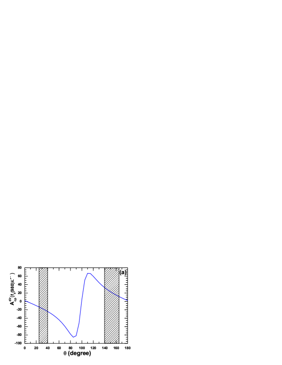
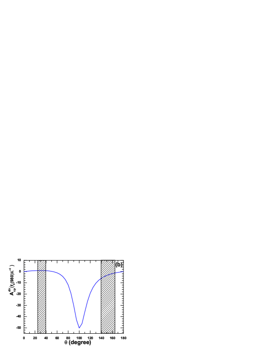
Figure 3: The $\theta$ dependence of the direct CP asymmetry (in units of percent) of the decays (a) $B^{-}\to f_{0}(980)K^{*-}$ and (b) $\bar{B}^{0}\to f_{0}(980)\bar{K}^{*0}$. The vertical bands show possible ranges of $\theta$: $25^{\circ}<\theta<40^{\circ}$ and $140^{\circ}<\theta<165^{\circ}$.

For the decay $\bar{B}^{0}\to f_{0}(s\bar{s})\bar{K}^{*0}$, there is no tree contribution at the leading order, so the CP asymmetry is naturally zero. But the CP asymmetry of $\bar{B}^{0}\to f_{0}(n\bar{n})\bar{K}^{*0}$ is large, for the $f_{0}$ emission non-factorizable diagrams (Fig.1(c) and (d)) give the large tree contributions, and its the direct CP asymmetry is about $-39\%$. It is similar to the decay $B^{-}\to f_{0}(980)K^{*-}$. From the Fig.3(a), one can find that if taking the mixing angle $25^{\circ}<\theta<40^{\circ}$, the direct CP asymmetry of the decay $B^{-}\to f_{0}(980)K^{*-}$ is:

$${\cal A}^{dir}_{CP}(B^{-}\to f_{0}(980)K^{*-})=(-15\sim-25)\%,$$ (60)

which may suffice to explain the experimental result pdg08 :

$${\cal A}^{dir}_{CP}(B^{-}\to f_{0}(980)K^{*-})=(-34\pm 21)\%.$$ (61)

But if we take the mixing angle $140^{\circ}<\theta<165^{\circ}$, the value has the opposite sign with the experimental result and becomes $(10\sim 33)\%$. Certainly, the errors from both the experimental result and the prediction are large.

From the upper analysis to the branch ratios of the decays $\bar{B}^{0}\to f_{0}(980)\bar{K}^{*0}$, $B^{-}\to f_{0}(980)K^{*-}$, it supports the conclusion that the mixing angle should be in the range of $140^{\circ}<\theta<165^{\circ}$. But unfortunately the range of $25^{\circ}<\theta<40^{\circ}$ as it seems cannot be ruled out absolutely. From Fig.2 and Fig.3, one can find there exist some symmetries for these two angle ranges. Within (large) theoretical errors, the results for the two angle ranges are both in agreement with the data. For example, if we take the angle $25^{\circ}<\theta<40^{\circ}$ in the Fig.3(b), the direct CP asymmetry of the decay $B^{-}\to f_{0}(980)K^{*-}$ is:

$${\cal A}^{dir}_{CP}(B^{-}\to f_{0}(980)K^{*-})=(0.8\sim 0.9)\%,$$ (62)

and ${\cal A}^{dir}_{CP}(B^{-}\to f_{0}(980)K^{*-})=(-1.2\sim-5.9)\%$ for $140^{\circ}<\theta<165^{\circ}$. That is to say the values of ${\cal A}^{dir}_{CP}(B^{-}\to f_{0}(980)K^{*-})$ for these two $\theta$ angle ranges are close and both small.

V Conclusion

In this paper, we calculate the branching ratios and CP-violating asymmetries of $\bar{B}^{0}\to f_{0}(980)\bar{K}^{*0}$ and $B^{-}\to f_{0}(980)K^{*-}$ decays in the pQCD factorization approach by identifying $f_{0}(980)$ as the composition of $s\bar{s}$ and $n\bar{n}=(u\bar{u}+d\bar{d})/\sqrt{2}$. Using the decay constants and light-cone distribution amplitude derived from the QCD sum-rule method, we find that:

• After including the twist-2 distribution amplitude and using the asymptotic form of twist-3 distribution amplitude, our results are larger than the previous pQCD predictions and can explain the present experimental data or the upper limit.

• From the results, it indicates that the contributions from the non-factorizable $f_{0}$ emission type diagrams are large, at the same time this type amplitude is sensitive to the shape of the distribution amplitudes.

• The branching ratio of $B\to f_{0}(980)K^{*}$ depends on the mixing angle $\theta$ of strange and nonstrange components of the $f_{0}(980)$. One can find that there exit some symmetries for the values in the two angle ranges (i.e., $25^{\circ}<\theta<40^{\circ}$ and $140^{\circ}<\theta<165^{\circ}$). So it is difficult to confirm the value of the mixing angle, unless we can get enough and precise experimental data.

• For the neutral decay $\bar{B}^{0}\to f_{0}(980)\bar{K}^{*0}$, we predict that the direct CP-violating asymmetry is small, only a few percent, which can be tested by the future B factory experiments.

References

(1)
A. Garmash et al. (Belle Collaboration), Phys. Rev. D 65, 092005 (2002).
(2)
N.A. Tornqvist, Phys. Rev. Lett. 49, 624 (1982).
(3) G.L. Jaffe, Phys. Rev. D 15, 267 (1977); Erratum-ibid.Phys. Rev. D 15 281 (1977);
A.L. Kataev, Phys. Atom. Nucl. 68, 567 (2005);
A. Vijande, A. Valcarce, F. Fernandez and B. Silvestre-Brac,
Phys. Rev. D72, 034025 (2005).
(4)
J. Weinstein, N. Isgur, Phys. Rev. Lett. 48, 659 (1982); Phys. Rev. D 27, 588 (1983);
41, 2236 (1990);
M.P. Locher et al., Eur. Phys. J. C 4, 317 (1998).
(5)
V. Baru et al., Phys. Lett. B586, 53 (2004).
(6)L. Celenza et al., Phys. Rev. C 61, 035201 (2000).
(7) M. Strohmeier-Presicek, et al., Phys. Rev. D 60, 054010 (1999).
(8) F.E. Close, A. Kirk, Phys. Lett. B 483, 345 (2000).
(9)
A.K. Giri , B. Mawlong , R. Mohanta, Phys. Rev. D 74, 114001 (2006).
(12)
H.Y. Cheng, C.K. Chua and K.C. Yang, Phys. Rev. D 77, 014034 (2008).
(13)
C.H. Cheng, Phys. Rev. D 67, 014012 (2003).
(14) C.H. Cheng, Phys. Rev. D 67, 094011 (2003).
(15)
W. Wang , Y.L. Shen , Y. Li , C.D. Lü Phys. Rev. D 74, 114010 (2006).
(16)
Z.Q. Zhang and Z.J. Xiao, Chin. Phys. C 33,7:508-515 (2009).
(17)
O. Abreu et al. (DELPHI Collaboration), Phys. Lett. B 449, 364 (1999);
A. Aloisio et al. (KLOE Collaboration), Phys. Lett. B 537, 21 (2002);
M.N. Achasov et al., Phys. Lett. B 485, 349 (2000).
(18)A.V. Anisovich, V.V. Anisovich, and V. A. Nikonov, Eur.
Phys. J. A 12, 103 (2001); Phys. At. Nucl. 65, 497 (2002).
(19)R. Kami nski, L. Le sniak, and B. Loiseau, Eur. Phys. J. C 9, 141 (1999).
(20)
A. Garmashet al. (Belle Collaboration), Phys. Rev. D 71, 092003
(2005).
(21) A. Garmash et al. (Belle Collaboration), Phys. Rev. Lett. 96, 251803 (2006), Phys. Rev. Lett. 94, 041802 (2005).