Efficient Learning with Partially Observed Attributes

Abstract

We describe and analyze efficient algorithms for learning a linear predictor from examples when the learner can only view a few attributes of each training example. This is the case, for instance, in medical research, where each patient participating in the experiment is only willing to go through a small number of tests. Our analysis bounds the number of additional examples sufficient to compensate for the lack of full information on each training example. We demonstrate the efficiency of our algorithms by showing that when running on digit recognition data, they obtain a high prediction accuracy even when the learner gets to see only four pixels of each image.

1 Introduction

Suppose we would like to predict if a person has some disease based on medical tests. Theoretically, we may choose a sample of the population, perform a large number of medical tests on each person in the sample and learn from this information. In many situations this is unrealistic, since patients participating in the experiment are not willing to go through a large number of medical tests. The above example motivates the problem studied in this paper, that is learning when there is a hard constraint on the number of attributes the learner may view for each training example.

We propose an efficient algorithm for dealing with this partial information problem, and bound the number of additional training examples sufficient to compensate for the lack of full information on each training example. Roughly speaking, we actively pick which attributes to observe in a randomized way so as to construct a “noisy” version of all attributes. Intuitively, we can still learn despite the error of this estimate because instead of receiving the exact value of each individual example in a small set it suffices to get noisy estimations of many examples.

1.1 Related Work

Many methods have been proposed for dealing with missing or partial information. Most of the approaches do not come with formal guarantees on the risk of the resulting algorithm, and are not guaranteed to converge in polynomial time. The difficulty stems from the exponential number of ways to complete the missing information. In the framework of generative models, a popular approach is the Expectation-Maximization (EM) procedure (Dempster et al., 1977). The main drawback of the EM approach is that it might find sub-optimal solutions. In contrast, the methods we propose in this paper are provably efficient and come with finite sample guarantees on the risk.

Our technique for dealing with missing information borrows ideas from algorithms for the adversarial multi-armed bandit problem (Auer et al., 2003; Cesa-Bianchi and Lugosi, 2006). Our learning algorithms actively choose which attributes to observe for each example. This and similar protocols were studied in the context of active learning (Cohn et al., 1994; Balcan et al., 2006; Hanneke, 2007, 2009; Beygelzimer et al., 2009), where the learner can ask for the target associated with specific examples.

The specific learning task we consider in the paper was first proposed in (Ben-David and Dichterman, 1998), where it is called “learning with restricted focus of attention”. Ben-David and Dichterman (1998) considered the classification setting and showed learnability of several hypothesis classes in this model, like $k$-DNF and axis-aligned rectangles. However, to the best of our knowledge, no efficient algorithm for the class of linear predictors has been proposed.

A related setting, called budgeted learning, was recently studied - see for example (Deng et al., 2007; Kapoor and Greiner, 2005) and the references therein. In budgeted learning, the learner purchases attributes at some fixed cost subject to an overall budget. Besides lacking formal guarantees, this setting is different from the one we consider in this paper, because we impose a budget constraint on the number of attributes that can be obtained for every individual example, as opposed to a global budget. In some applications, such as the medical application discussed previously, our constraint leads to a more realistic data acquisition process - the global budget allows to ask for many attributes of some individual patients while our protocol guarantees a constant number of medical tests to all the patients.

Our technique is reminiscent of methods used in the compressed learning framework (Calderbank et al., 2009; Zhou et al., 2009), where data is accessed via a small set of random linear measurements. Unlike compressed learning, where learners are both trained and evaluated in the compressed domain, our techniques are mainly designed for a scenario in which only the access to training data is restricted.

The “opposite” setting, in which full information is given at training time and the goal is to train a predictor that depends only on a small number of attributes at test time, was studied in the context of learning sparse predictors - see for example (Tibshirani, 1996) and the wide literature on sparsity properties of $\ell_{1}$ regularization. Since our algorithms also enforce low $\ell_{1}$ norm, many of those results can be combined with our techniques to yield an algorithm that views only $O(1)$ attributes at training time, and a number of attributes comparable to the achievable sparsity at test time. Since our focus in this work is on constrained information at training time, we do not elaborate on this subject. Furthermore, in some real-world situations, it is reasonable to assume that attributes are very expensive at training time but are more easy to obtain at test time. Returning to the example of medical applications, it is unrealistic to convince patients to participate in a medical experiment in which they need to go through a lot of medical tests, but once the system is trained, at testing time, patients who need the prediction of the system will agree to perform as many medical tests as needed.

A variant of the above setting is the one studied by Greiner et al. (2002), where the learner has all the information at training time and at test time he tries to actively choose a small amount of attributes to form a prediction. Note that active learning at training time, as we do here, may give more learning power than active learning at testing time. For example, we formally prove that while it is possible to learn a consistent predictor accessing at most $2$ attributes of each example at training time, it is not possible (even with an infinite amount of training examples) to build an active classifier that uses at most $2$ attributes of each example at test time, and whose error will be smaller than a constant.

2 Main Results

In this section we outline the main results. We start with a formal description of the learning problem. In linear regression each example is an instance-target pair, $({\mathbf{x}},y)\in\mathbb{R}^{d}\times\mathbb{R}$. We refer to ${\mathbf{x}}$ as a vector of attributes and the goal of the learner is to find a linear predictor ${\mathbf{x}}\mapsto\langle{\mathbf{w}},{\mathbf{x}}\rangle$, where we refer to ${\mathbf{w}}\in\mathbb{R}^{d}$ as the predictor. The performance of a predictor ${\mathbf{w}}$ on an instance-target pair, $({\mathbf{x}},y)\in\mathbb{R}^{d}\times\mathbb{R}$, is measured by a loss function $\ell(\langle{\mathbf{w}},{\mathbf{x}}\rangle,y)$. For simplicity, we focus on the squared loss function, $\ell(a,b)=(a-b)^{2}$, and briefly discuss other loss functions in Section 5. Following the standard framework of statistical learning (Haussler, 1992; Devroye et al., 1996; Vapnik, 1998), we model the environment as a joint distribution $\mathcal{D}$ over the set of instance-target pairs, $\mathbb{R}^{d}\times\mathbb{R}$. The goal of the learner is to find a predictor with low risk, defined as the expected loss: $L_{\mathcal{D}}({\mathbf{w}})~{}\stackrel{{\scriptstyle\mathrm{def}}}{{=}}~{}\operatorname*{\mathbb{E}}_{({\mathbf{x}},y)\sim\mathcal{D}}[\ell(\langle{\mathbf{w}},{\mathbf{x}}\rangle,y)]$. Since the distribution $\mathcal{D}$ is unknown to the learner he learns by relying on a training set of $m$ examples $S=({\mathbf{x}}_{1},y_{1}),\ldots,({\mathbf{x}}_{m},y_{m})$, which are assumed to be sampled i.i.d. from $\mathcal{D}$. We denote the training loss by $L_{S}({\mathbf{w}})\stackrel{{\scriptstyle\mathrm{def}}}{{=}}\frac{1}{m}\sum_{i=1}^{m}(\langle{\mathbf{w}},{\mathbf{x}}_{i}\rangle-y_{i})^{2}$. We now distinguish between two scenarios:

• Full information: The learner receives the entire training set. This is the traditional linear regression setting.

• Partial information: For each individual example, $({\mathbf{x}}_{i},y_{i})$, the learner receives the target $y_{i}$ but is only allowed to see $k$ attributes of ${\mathbf{x}}_{i}$, where $k$ is a parameter of the problem. The learner has the freedom to actively choose which of the attributes will be revealed, as long as at most $k$ of them will be given.

While the full information case was extensively studied, the partial information case is more challenging. Our approach for dealing with the problem of partial information is to rely on algorithms for the full information case and to fill in the missing information in a randomized, data and algorithmic dependent, way. As a simple baseline, we begin by describing a straightforward adaptation of Lasso (Tibshirani, 1996), based on a direct nonadaptive estimate of the loss function. We then turn to describe a more effective approach, which combines a stochastic gradient descent algorithm called Pegasos (Shalev-Shwartz et al., 2007) with the active sampling of attributes in order to estimate the gradient of the loss at each step.

2.1 Baseline Algorithm

A popular approach for learning a linear regressor is to minimize the empirical loss on the training set plus a regularization term taking the form of a norm of the predictor. For example, in ridge regression the regularization term is $\|{\mathbf{w}}\|_{2}^{2}$ and in Lasso the regularization term is $\|{\mathbf{w}}\|_{1}$. Instead of regularization, we can include a constraint of the form $\|{\mathbf{w}}\|_{1}\leq B$ or $\|{\mathbf{w}}\|_{2}\leq B$. With an adequate tuning of parameters, the regularization form is equivalent to the constraint form. In the constraint form, the predictor is a solution to the following optimization problem:

$$\min_{{\mathbf{w}}\in\mathbb{R}^{d}}~{}\tfrac{1}{|S|}\sum_{({\mathbf{x}},y)\in S}(\langle{\mathbf{w}},{\mathbf{x}}\rangle-y)^{2}~{}~{}\textrm{s.t.}~{}~{}\|{\mathbf{w}}\|_{p}\leq B~{},$$ (1)

where $S=\{({\mathbf{x}}_{1},y_{1}),\ldots,({\mathbf{x}}_{m},y_{m})\}$ is a training set of examples, $B$ is a regularization parameter, and $p$ is $1$ for Lasso and $2$ for ridge regression. Standard risk bounds for Lasso imply that if $\hat{{\mathbf{w}}}$ is a minimizer of (1) (with $p=1$), then with probability greater than $1-\delta$ over the choice of a training set of size $m$ we have

$$L_{\mathcal{D}}(\hat{{\mathbf{w}}})\leq\min_{{\mathbf{w}}:\|{\mathbf{w}}\|_{1}\leq B}L_{D}({\mathbf{w}})+O\left(\!\!B^{2}\,\sqrt{\frac{\ln(d/\delta)}{m}}\right)~{}.$$ (2)

To adapt Lasso to the partial information case, we first rewrite the squared loss as follows:

$$(\langle{\mathbf{w}},{\mathbf{x}}\rangle-y)^{2}={\mathbf{w}}^{T}({\mathbf{x}}{\mathbf{x}}^{T}){\mathbf{w}}-2y{\mathbf{x}}^{T}{\mathbf{w}}+y^{2}~{},$$

where ${\mathbf{w}},{\mathbf{x}}$ are column vectors and ${\mathbf{w}}^{T},{\mathbf{x}}^{T}$ are their corresponding transpose (i.e., row vectors). Next, we estimate the matrix ${\mathbf{x}}{\mathbf{x}}^{T}$ and the vector ${\mathbf{x}}$ using the partial information we have, and then we solve the optimization problem given in (1) with the estimated values of ${\mathbf{x}}{\mathbf{x}}^{T}$ and ${\mathbf{x}}$. To estimate the vector ${\mathbf{x}}$ we can pick an index $i$ uniformly at random from $[d]=\{1,\ldots,d\}$ and define the estimation to be a vector ${\mathbf{v}}$ such that

$${v}_{r}~{}=~{}\begin{cases}d\,x_{r}&\textrm{if}~{}r=i\\ 0&\textrm{else}\end{cases}~{}~{}~{}.$$ (3)

It is easy to verify that ${\mathbf{v}}$ is an unbiased estimate of ${\mathbf{x}}$, namely, $\operatorname*{\mathbb{E}}[{\mathbf{v}}]={\mathbf{x}}$ where expectation is with respect to the choice of the index $i$. When we are allowed to see $k>1$ attributes, we simply repeat the above process (without replacement) and set ${\mathbf{v}}$ to be the averaged vector. To estimate the matrix ${\mathbf{x}}{\mathbf{x}}^{T}$ we could pick two indices $i,j$ independently and uniformly at random from $[d]$, and define the estimation to be a matrix with all zeros except $d^{2}\,x_{i}x_{j}$ in the $(i,j)$ entry. However, this yields a non-symmetric matrix which will make our optimization problem with the estimated matrix non-convex. To overcome this obstacle, we symmetrize the matrix by adding its transpose and dividing by $2$. The resulting baseline procedure is given in Algorithm 1.

Algorithm 1 Baseline$(S,k)$
$S$ — full information training set with $m$ examples
$k$ — Can view only $k$ elements of each instance in $S$
Parameter: $B$

	Initialize: $\bar{A}=\boldsymbol{0}\in\mathbb{R}^{d,d}$  ;  $\bar{{\mathbf{v}}}=\boldsymbol{0}\in\mathbb{R}^{d}$  ;  $\bar{y}=0$
for each $({\mathbf{x}},y)\in S$
${\mathbf{v}}=\boldsymbol{0}\in\mathbb{R}^{d}$
${A}=\boldsymbol{0}\in\mathbb{R}^{d,d}$
Choose $C$ uniformly at random from
all subsets of $[d]\times[d]$ of size $k/2$
for each $(i,j)\in C$
$v_{i}=v_{i}+(d/k)\,x_{i}$
$v_{j}=v_{j}+(d/k)\,x_{j}$
${A}_{i,j}={A}_{i,j}+(d^{2}/k)\,x_{i}x_{j}$
${A}_{j,i}={A}_{j,i}+(d^{2}/k)\,x_{i}x_{j}$
end
$\bar{A}=\bar{A}+A/m$
$\bar{{\mathbf{v}}}=\bar{{\mathbf{v}}}+2\,y\,{\mathbf{v}}/m$
$\bar{y}=\bar{y}+y^{2}/m$
end
Let $\tilde{L}_{S}({\mathbf{w}})={\mathbf{w}}^{T}\bar{A}{\mathbf{w}}+{\mathbf{w}}^{T}\,\bar{{\mathbf{v}}}+\bar{y}$
Output: solution of $\displaystyle\min_{{\mathbf{w}}:\|{\mathbf{w}}\|_{1}\leq B}\tilde{L}_{S}({\mathbf{w}})$

The following theorem shows that similar to Lasso, the Baseline algorithm is competitive with the optimal linear predictor with a bounded $L_{1}$ norm.

Theorem 1

Let $\mathcal{D}$ be a distribution such that $\operatorname*{\mathbb{P}}[{\mathbf{x}}\in[-1,+1]^{d}\land y\in[-1,+1]]=1$. Let $\hat{{\mathbf{w}}}$ be the output of Baseline(S,k), where $|S|=m$. Then, with probability of at least $1-\delta$ over the choice of the training set and the algorithm’s own randomization we have

$$L_{\mathcal{D}}(\hat{{\mathbf{w}}})\leq\min_{{\mathbf{w}}:\|{\mathbf{w}}\|_{1}\leq B}L_{D}({\mathbf{w}})+O\left(\frac{(d\,B)^{2}}{k}\,\sqrt{\frac{\ln(d/\delta)}{m}}\right)~{}.$$

The above theorem tells us that for a sufficiently large training set we can find a very good predictor. Put another way, a large number of examples can compensate for the lack of full information on each individual example. In particular, to overcome the extra factor $d^{2}/k$ in the bound, which does not appear in the full information bound given in (2), we need to increase $m$ by a factor of $d^{4}/k^{2}$.

Note that when $k=d$ we do not recover the full information bound. This is because we try to estimate a matrix with $d^{2}$ entries using only $k=d<d^{2}$ samples. In the next subsection, we describe a better, adaptive procedure for the partial information case.

2.2 Gradient-based Attribute Efficient Regression

In this section, by avoiding the estimation of the matrix ${\mathbf{x}}{\mathbf{x}}^{T}$, we significantly decrease the number of additional examples sufficient for learning with $k$ attributes per training example. To do so, we do not try to estimate the loss function but rather estimate the gradient $\nabla\ell({\mathbf{w}})~{}=~{}2\,(\langle{\mathbf{w}},{\mathbf{x}}\rangle-y)\,{\mathbf{x}}$, with respect to ${\mathbf{w}}$, of the squared loss function $(\langle{\mathbf{w}},{\mathbf{x}}\rangle-y)^{2}$. Each vector ${\mathbf{w}}$ can define a probability distribution over $[d]$ by letting $\operatorname*{\mathbb{P}}[i]=|w_{i}|/\|{\mathbf{w}}\|_{1}$. We can estimate the gradient using $2$ attributes as follows. First, we randomly pick $j$ from $[d]$ according to the distribution defined by ${\mathbf{w}}$. Using $j$ we estimate the term $\langle{\mathbf{w}},{\mathbf{x}}\rangle$ by ${\mathrm{sgn}}(w_{j})\,\|{\mathbf{w}}\|_{1}\,x_{j}$. It is easy to verify that the expectation of the estimate equals $\langle{\mathbf{w}},{\mathbf{x}}\rangle$. Second, we randomly pick $i$ from $[d]$ according to the uniform distribution over $[d]$. Based on $i$, we estimate the vector ${\mathbf{x}}$ as in (3). Overall, we obtain the following unbiased estimation of the gradient:

$$\tilde{\nabla}\ell({\mathbf{w}})~{}=~{}2\,({\mathrm{sgn}}(w_{j})\,\|{\mathbf{w}}\|_{1}\,x_{j}-y)\,{\mathbf{v}}~{},$$ (4)

where ${\mathbf{v}}$ is as defined in (3).

The advantage of the above approach over the loss based approach we took before is that the magnitude of each element of the gradient estimate is order of $d\,\|{\mathbf{w}}\|_{1}$. This is in contrast to what we had for the loss based approach, where the magnitude of each element of the matrix $A$ was order of $d^{2}$. In many situations, the $L_{1}$ norm of a good predictor is significantly smaller than $d$ and in these cases the gradient based estimate is better than the loss based estimate. However, while in the previous approach our estimation did not depend on a specific ${\mathbf{w}}$, now the estimation depends on ${\mathbf{w}}$. We therefore need an iterative learning method in which at each iteration we use the gradient of the loss function on an individual example. Luckily, the stochastic gradient descent approach conveniently fits our needs.

Concretely, below we describe a variant of the Pegasos algorithm (Shalev-Shwartz et al., 2007) for learning linear regressors. Pegasos tries to minimize the regularized risk

$$\min_{\mathbf{w}}~{}~{}\operatorname*{\mathbb{E}}_{({\mathbf{x}},y)\sim\mathcal{D}}\left[(\langle{\mathbf{w}},{\mathbf{x}}\rangle-y)^{2}\right]+\lambda\|{\mathbf{w}}\|_{2}^{2}~{}.$$ (5)

Of course, the distribution $\mathcal{D}$ is unknown, and therefore we cannot hope to solve the above problem exactly. Instead, Pegasos finds a sequence of weight vectors that (on average) converge to the solution of (5). We start with the all zeros vector ${\mathbf{w}}=\boldsymbol{0}\in\mathbb{R}^{d}$. Then, at each iteration Pegasos picks the next example in the training set (which is equivalent to sampling a fresh example according to $\mathcal{D}$) and calculates the gradient of the loss function on this example with respect to the current weight vector ${\mathbf{w}}$. In our case, the gradient is simply $2(\langle{\mathbf{w}},{\mathbf{x}}\rangle-y){\mathbf{x}}$. We denote this gradient vector by $\nabla$. Finally, Pegasos updates the predictor according to the rule: ${\mathbf{w}}=(1-\tfrac{1}{t})\,{\mathbf{w}}-\frac{1}{\lambda\,t}\,\nabla$, where $t$ is the current iteration number.

To apply Pegasos in the partial information case we could simply replace the gradient vector $\nabla$ with its estimation given in (4). However, our analysis shows that it is desirable to maintain an estimation vector $\tilde{\nabla}$ with small magnitude. Since the magnitude of $\tilde{\nabla}$ is order of $d\,\|{\mathbf{w}}\|_{1}$, where ${\mathbf{w}}$ is the current weight vector maintained by the algorithm, we would like to ensure that $\|{\mathbf{w}}\|_{1}$ is always smaller than some threshold $B$. We achieve this goal by adding an additional projection step at the end of each Pegasos’s iteration. Formally, after performing the update we set

$${\mathbf{w}}\leftarrow\operatorname*{argmin}_{{\mathbf{u}}:\|{\mathbf{u}}\|_{1}\leq B}\|{\mathbf{u}}-{\mathbf{w}}\|_{2}~{}.$$ (6)

This projection step can be performed efficiently in time $O(d)$ using the technique described in (Duchi et al., 2008). A pseudo-code of the resulting Attribute Efficient Regression algorithm is given in Algorithm 2.

Algorithm 2 AER$(S,k)$
$S$ — Full information training set with $m$ examples
$k$ — Access only $k$ elements of each instance in $S$
Parameters: $\lambda,B$

	${\mathbf{w}}=(0,\ldots,0)$  ;  $\bar{{\mathbf{w}}}={\mathbf{w}}$  ;  $t=1$
for each $({\mathbf{x}},y)\in S$
${\mathbf{v}}=\boldsymbol{0}\in\mathbb{R}^{d}$
Choose $C$ uniformly at random from
all subsets of $[d]$ of size $k/2$
for each $j\in C$
$v_{j}=v_{j}+\tfrac{2}{k}\,d\,x_{j}$
end
$\hat{y}=0$
for $r=1,\ldots,k/2$
sample $i$ from $[d]$ based on $\operatorname*{\mathbb{P}}[i]=|w_{i}|/\|{\mathbf{w}}\|_{1}$
$\hat{y}=\hat{y}+\tfrac{2}{k}\,{\mathrm{sgn}}(w_{i})\,\|{\mathbf{w}}\|_{1}\,x_{j}$
end
${\mathbf{w}}=(1-\tfrac{1}{t}){\mathbf{w}}-\tfrac{2}{\lambda t}(\hat{y}-y){\mathbf{v}}$
${\mathbf{w}}=\operatorname*{argmin}_{{\mathbf{u}}:\|{\mathbf{u}}\|_{1}\leq B}\|{\mathbf{u}}-{\mathbf{w}}\|_{2}$
$\bar{{\mathbf{w}}}=\bar{{\mathbf{w}}}+{\mathbf{w}}/m$
$t=t+1$
end
Output: $\bar{{\mathbf{w}}}$

The following theorem provides convergence guarantees for AER.

Theorem 2

Let $\mathcal{D}$ be a distribution such that $\operatorname*{\mathbb{P}}[{\mathbf{x}}\in[-1,+1]^{d}\land y\in[-1,+1]]=1$. Let ${\mathbf{w}}^{\star}$ be any vector such that $\|{\mathbf{w}}^{\star}\|_{1}\leq B$ and $\|{\mathbf{w}}^{\star}\|_{2}\leq B_{2}$ Then,

$$\operatorname*{\mathbb{E}}[L_{\mathcal{D}}(\bar{{\mathbf{w}}})]~{}\leq~{}L_{\mathcal{D}}({\mathbf{w}}^{\star})+O\left(\frac{d\,(B+1)\,B_{2}}{\sqrt{k}}\,\sqrt{\frac{\ln(m)}{m}}\right)~{},$$

where $|S|=m$, $\bar{{\mathbf{w}}}$ is the output of AER$(S,k)$ run with $\lambda=((B+1)d/B_{2})\,\sqrt{\log(m)/(mk)}$, and the expectation is over the choice of $S$ and over the algorithm’s own randomization.

For simplicity and readability, in the above theorem we only bounded the expected risk. It is possible to obtain similar guarantees with high probability by relying on Azuma’s inequality —see for example (Cesa-Bianchi et al., 2004).

Note that $\|{\mathbf{w}}^{\star}\|_{2}\leq\|{\mathbf{w}}^{\star}\|_{1}\leq B$, so Theorem 2 implies that

$$L_{\mathcal{D}}(\bar{{\mathbf{w}}})\leq\min_{{\mathbf{w}}:\|{\mathbf{w}}\|_{1}\leq B}L_{D}({\mathbf{w}})+O\left(\frac{d\,B^{2}}{\sqrt{k}}\,\sqrt{\frac{\ln(m)}{m}}\right)~{}.$$

Therefore, the bound for AER is much better than the bound for Baseline: instead of $d^{2}/k$ we have $d/\sqrt{k}$.

It is interesting to compare the bound for AER to the Lasso bound in the full information case given in (2). As it can be seen, to achieve the same level of risk, AER needs a factor of $d^{2}/k$ more examples than the full information Lasso. Since each AER example uses only $k$ attributes while each Lasso example uses all $d$ attributes, the ratio between the total number of attributes AER needs and the number of attributes Lasso needs to achieve the same error is $O(d)$. Intuitively, when having $d$ times total number of attributes, we can fully compensate for the partial information protocol.

However, in some situations even this extra $d$ factor is not needed. Suppose we know that the vector ${\mathbf{w}}^{\star}$, which minimizes the risk, is dense. That is, it satisfies $\|{\mathbf{w}}^{\star}\|_{1}\approx\sqrt{d}\,\|{\mathbf{w}}^{\star}\|_{2}$. In this case, choosing $B_{2}=B/\sqrt{d}$, the bound in Theorem 2 becomes order of $B^{2}\sqrt{d/k}\sqrt{1/m}$. Therefore, the number of examples AER needs in order to achieve the same error as Lasso is only a factor $d/k$ more than the number of examples Lasso uses. But, this implies that both AER and Lasso needs the same number of attributes in order to achieve the same level of error! Crucially, the above holds only if ${\mathbf{w}}^{\star}$ is dense. When ${\mathbf{w}}^{\star}$ is sparse we have $\|{\mathbf{w}}^{\star}\|_{1}\approx\|{\mathbf{w}}^{\star}\|_{2}$ and then AER needs more attributes than Lasso.

One might wonder whether a more clever active sampling strategy could attain in the sparse case the performance of Lasso while using the same number of attributes. The next subsection shows that this is not possible in general.

2.3 Lower bounds and negative results

We now show (proof in the appendix) that any attribute efficient algorithm needs in general order of $d/\epsilon$ examples for learning an $\epsilon$-accurate sparse linear predictor. Recall that the upper bound of AER implies that order of $d^{2}(B+1)^{2}B_{2}^{2}/\epsilon^{2}$ examples are sufficient for learning a predictor with $L_{\mathcal{D}}({\mathbf{w}})-L_{\mathcal{D}}({\mathbf{w}}^{\star})<\epsilon$. Specializing this sample complexity bound of AER to the ${\mathbf{w}}^{\star}$ described in Theorem 3 below, yields that $O(d^{2}/\epsilon)$ examples are sufficient for AER for learning a good predictor in this case. That is, we have a gap of factor $d$ between the lower bound and the upper bound, and it remains open to bridge this gap.

Theorem 3

For any $\epsilon\in(0,1/16)$, $k$, and $d\geq 4k$, there exists a distribution over examples and a weight vector ${\mathbf{w}}^{\star}$, with $\|{\mathbf{w}}^{\star}\|_{0}=1$ and $\|{\mathbf{w}}^{\star}\|_{2}=\|{\mathbf{w}}^{\star}\|_{1}=2\sqrt{\epsilon}$, such that any attribute efficient regression algorithm accessing at most $k$ attributes per training example must see (in expectation) at least $\Omega\left(\tfrac{d}{k\epsilon}\right)$ examples in order to learn a linear predictor ${\mathbf{w}}$ with $L_{\mathcal{D}}({\mathbf{w}})-L_{\mathcal{D}}({\mathbf{w}}^{\star})<\epsilon$.

Recall that in our setting, while at training time the learner can only view $k$ attributes of each example, at test time all attributes can be observed. The setting of Greiner et al. (2002), instead, assumes that at test time the learner cannot observe all the attributes. The following theorem shows that if a learner can view at most $2$ attributes at test time then it is impossible to give accurate predictions at test time even when the optimal linear predictor is known.

Theorem 4

There exists a weight vector ${\mathbf{w}}^{\star}$ and a distribution $\mathcal{D}$ such that $L_{\mathcal{D}}({\mathbf{w}}^{\star})=0$ while any algorithm $A$ that gives predictions $A({\mathbf{x}})$ while viewing only $2$ attributes of each ${\mathbf{x}}$ must have $L_{\mathcal{D}}(A)\geq 1/9$.

The proof is given in the appendix. This negative result highlights an interesting phenomenon. We can learn an arbitrarily accurate predictor ${\mathbf{w}}$ from partially observed examples. However, even if we know the optimal ${\mathbf{w}}^{\star}$, we might not be able to accurately predict a new partially observed example.

3 Proof Sketch of Theorem 2

Here we only sketch the proof of Theorem 2. A complete proof of all our theorems is given in the appendix.

We start with a general logarithmic regret bound for strongly convex functions (Hazan et al., 2006; Kakade and Shalev-Shwartz, 2008). The regret bound implies the following. Let ${\mathbf{z}}_{1},\ldots,{\mathbf{z}}_{m}$ be a sequence of vectors, each of which has norm bounded by $G$. Let $\lambda>0$ and consider the sequence of functions $g_{1},\ldots,g_{m}$ such that $g_{t}({\mathbf{w}})=\tfrac{\lambda}{2}\|{\mathbf{w}}\|^{2}+\langle{\mathbf{z}}_{t},{\mathbf{w}}\rangle$. Each $g_{t}$ is $\lambda$-strongly convex (meaning, it is not too flat), and therefore regret bounds for strongly convex functions tell us that there is a way to construct a sequence of vectors ${\mathbf{w}}_{1},\ldots,{\mathbf{w}}_{m}$ such that for any ${\mathbf{w}}^{\star}$ that satisfies $\|{\mathbf{w}}^{\star}\|_{1}\leq B$ we have

$$\frac{1}{t}\sum_{t=1}^{m}g_{t}({\mathbf{w}}_{t})-\frac{1}{t}\sum_{t=1}^{m}g_{t}({\mathbf{w}}^{\star})\leq O\left(\tfrac{G^{2}\,\log(m)}{\lambda\,m}\right)~{}.$$

With an appropriate choice of $\lambda$, and with the assumption $\|{\mathbf{w}}^{\star}\|_{2}\leq B_{2}$, the above inequality implies that $\tfrac{1}{m}\sum_{t=1}^{m}\langle{\mathbf{z}}_{t},{\mathbf{w}}_{t}-{\mathbf{w}}^{\star}\rangle\leq\alpha$ where $\alpha=O\left(\tfrac{G\,B_{2}\,\log(m)}{\sqrt{m}}\right)$. This holds for any sequence of ${\mathbf{z}}_{1},\ldots,{\mathbf{z}}_{m}$, and in particular, we can set ${\mathbf{z}}_{t}=2(\hat{y}_{t}-y_{t}){\mathbf{v}}_{t}$. Note that ${\mathbf{z}}_{t}$ is a random vector that depends both on the value of ${\mathbf{w}}_{t}$ and on the random bits chosen on round $t$. Taking conditional expectation of ${\mathbf{z}}_{t}$ w.r.t. the random bits chosen on round $t$ we obtain that $\operatorname*{\mathbb{E}}[{\mathbf{z}}_{t}|{\mathbf{w}}_{t}]$ is exactly the gradient of $(\langle{\mathbf{w}},{\mathbf{x}}_{t}\rangle-y_{t})^{2}$ at ${\mathbf{w}}_{t}$, which we denote by $\nabla_{t}$. From the convexity of the squared loss, we can lower bound $\langle\nabla_{t},{\mathbf{w}}_{t}-{\mathbf{w}}^{\star}\rangle$ by $(\langle{\mathbf{w}}_{t},{\mathbf{x}}_{t}\rangle-y_{t})^{2}-(\langle{\mathbf{w}}^{\star},{\mathbf{x}}_{t}\rangle-y_{t})^{2}$. That is, in expectation we have that

$$\operatorname*{\mathbb{E}}\left[\tfrac{1}{m}\sum_{t=1}^{m}\left((\langle{\mathbf{w}}_{t},{\mathbf{x}}_{t}\rangle-y_{t})^{2}-(\langle{\mathbf{w}}^{\star},{\mathbf{x}}_{t}\rangle-y_{t})^{2}\right)\right]\leq\alpha~{}.$$

Taking expectation w.r.t. the random choice of the examples from $\mathcal{D}$, denoting $\bar{{\mathbf{w}}}=\tfrac{1}{m}\sum_{t=1}^{m}$, and using Jensen’s inequality we get that $\operatorname*{\mathbb{E}}[L_{\mathcal{D}}(\bar{{\mathbf{w}}})]\leq L_{\mathcal{D}}({\mathbf{w}}^{\star})+\alpha$. Finally, we need to make sure that $\alpha$ is not too large. The only potential danger is that $G$, the bound on the norms of ${\mathbf{z}}_{1},\ldots,{\mathbf{z}}_{m}$, will be large. We make sure this cannot happen by restricting each ${\mathbf{w}}_{t}$ to the $\ell_{1}$ ball of radius $B$, which ensures that $\|{\mathbf{z}}_{t}\|\leq O((B+1)d)$ for all $t$.

4 Experiments

We performed some preliminary experiments to test the behavior of our algorithm on the well-known MNIST digit recognition dataset (Cun et al., 1998), which contains 70,000 images ($28\times 28$ pixels each) of the digits $0-9$. The advantages of this dataset for our purposes is that it is not a small-scale dataset, has a reasonable dimensionality-to-data-size ratio, and the setting is clearly interpretable graphically. While this dataset is designed for classification (e.g. recognizing the digit in the image), we can still apply our algorithms on it by regressing to the label.

First, to demonstrate the hardness of our settings, we provide in Figure 1 below some examples of images from the dataset, in the full information setting and the partial information setting. The upper row contains six images from the dataset, as available to a full-information algorithm. A partial-information algorithm, however, will have a much more limited access to these images. In particular, if the algorithm may only choose $k=4$ pixels from each image, the same six images as available to it might look like the bottom row of Figure 1.

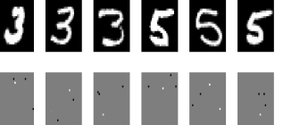
Figure 1: In the upper row six examples from the training set (of digits 3 and 5) are shown. In the lower row we show the same six examples, where only four randomly sampled pixels from each original image are displayed.

We began by looking at a dataset composed of “$3$ vs. $5$”, where all the $3$ digits were labeled as $-1$ and all the $5$ digits were labeled as $+1$. We ran four different algorithms on this dataset: the simple Baseline algorithm, AER, as well as ridge regression and Lasso for comparison (for Lasso, we solved (1) with $p=1$). Both ridge regression and Lasso were run in the full information setting: Namely, they enjoyed full access to all attributes of all examples in the training set. The Baseline algorithm and AER, however, were given access to only $4$ attributes from each training example.

We randomly split the dataset into a training set and a test set (with the test set being $10\%$ of the original dataset). For each algorithm, parameter tuning was performed using $10$-fold cross validation. Then, we ran the algorithm on increasingly long prefixes of the training set, and measured the average regression error $(\langle{\mathbf{w}},{\mathbf{x}}\rangle-y)^{2}$ on the test set. The results (averaged over runs on $10$ random train-test splits) are presented in Figure 2. In the upper plot, we see how the test regression error improves with the number of examples. The Baseline algorithm is highly unstable at the beginning, probably due to the ill-conditioning of the estimated covariance matrix, although it eventually stabilizes (to prevent a graphical mess at the left hand side of the figure, we removed the error bars from the corresponding plot). Its performance is worse than AER, completely in line with our earlier theoretical analysis.

The bottom plot of Figure 2 is similar, only that now the $X$-axis represents the accumulative number of attributes seen by each algorithm rather than the number of examples. For the partial-information algorithm, the graph ends at approximately 49,000 attributes, which is the total number of attributes accessed by the algorithm after running over all training examples, seeing $k=4$ pixels from each example. However, for the full-information algorithm 49,000 attributes are already seen after just $62$ examples. When we compare the algorithms in this way, we see that our AER algorithm achieves excellent performance for a given attribute budget, significantly better than the other $L_{1}$-based algorithms, and even comparable to full-information ridge regression.

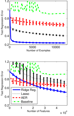
Figure 2: Test regression error for each of the $4$ algorithms, over increasing prefixes of the training set for “3 vs. 5”. The results are averaged over $10$ runs.

Finally, we tested the algorithms over $45$ datasets generated from MNIST, one for each possible pair of digits. For each dataset and each of $10$ random train-test splits, we performed parameter tuning for each algorithm separately, and checked the average squared error on the test set. The median test errors over all datasets are presented in the table below.

		Test Error
Full Information	Ridge	0.110
	Lasso	0.222
Partial Information	AER	0.320
	Baseline	0.815

As can be seen, the AER algorithm manages to achieve good performance, not much worse than the full-information Lasso algorithm. The Baseline algorithm, however, achieves a substantially worse performance, in line with our theoretical analysis above. We also calculated the test classification error of AER, i.e. $\text{sign}(\langle{\mathbf{w}},{\mathbf{x}}\rangle)\neq y$, and found out that AER, which can see only $4$ pixels per image, usually perform only a little worse than the full-information algorithms (ridge regression and Lasso), which enjoy full access to all $784$ pixels in each image. In particular, the median test classification errors of AER, Lasso, and Ridge are $3.5\%,~{}1.1\%,$ and $1.3\%$ respectively.

5 Discussion and Extensions

In this paper, we provided an efficient algorithm for learning when only a few attributes from each training example can be seen. The algorithm comes with formal guarantees, is provably competitive with algorithms which enjoy full access to the data, and seems to perform well in practice. We also presented sample complexity lower bounds, which are only a factor $d$ smaller than the upper bound achieved by our algorithm, and it remains open to bridge this gap.

Our approach easily extends to other gradient-based algorithms besides Pegasos. For example, generalized additive algorithms such as $p$-norm Perceptrons and Winnow - see, e.g., (Cesa-Bianchi and Lugosi, 2006).

An obvious direction for future research is how to deal with loss functions other than the squared loss. In upcoming work on a related problem, we develop a technique which allows us to deal with arbitrary analytic loss functions, but in the setting of this paper will lead to sample complexity bounds which are exponential in $d$. Another interesting extension we are considering is connecting our results to the field of privacy-preserving learning (Dwork, 2008), where the goal is to exploit the attribute efficiency property in order to prevent acquisition of information about individual data instances.

Appendix A Proofs

A.1 Proof of Theorem 1

To ease our calculations, we first show that sampling $k$ elements without replacements and then averaging the result has the same expectation as sampling just once. In the lemma below, for a set $C$ we denote the uniform distribution over $C$ by $U(C)$.

Lemma 1

Let $C$ be a finite set and let $f:C\to\mathbb{R}$ be an arbitrary function. Let $C_{k}=\{C^{\prime}\subset C:|C^{\prime}|=k\}$. Then,

$$\operatorname*{\mathbb{E}}_{C^{\prime}\sim U(C_{k})}[\tfrac{1}{k}\sum_{c\in C^{\prime}}f(c)]~{}=~{}\operatorname*{\mathbb{E}}_{c\sim U(C)}[f(c)]~{}.$$

Proof  Denote $|C|=n$. We have:

$$\begin{split}\operatorname*{\mathbb{E}}_{C^{\prime}\sim U(C_{k})}[&\tfrac{1}{k}\sum_{c\in C^{\prime}}f(c)]=\frac{1}{{n\choose k}}\sum_{C^{\prime}\in C_{k}}\tfrac{1}{k}\sum_{c\in C^{\prime}}f(c)\\ &=\frac{1}{k{n\choose k}}\sum_{c\in C}f(c)|\{C^{\prime}\in C_{k}:c\in C^{\prime}\}|\\ &=\frac{{n-1\choose k-1}}{k{n\choose k}}\sum_{c\in C}f(c)\\ &=\frac{(n-1)!k!(n-k)!}{kn!(k-1)!(n-k)!}\sum_{c\in C}f(c)\\ &=\frac{1}{n}\sum_{c\in C}f(c)\\ &=\operatorname*{\mathbb{E}}_{c\sim U(C)}[f(c)]~{}.\end{split}$$

 

To prove Theorem 1 we first show that the estimation matrix constructed by the Baseline algorithm is likely to be close to the true correlation matrix over the training set.

Lemma 2

Let $A_{t}$ be the matrix constructed at iteration $t$ of the Baseline algorithm and note that $\bar{A}=\frac{1}{m}\sum_{t=1}^{m}A_{t}$. Let $X=\frac{1}{m}\sum_{t=1}^{m}{\mathbf{x}}_{t}{\mathbf{x}}_{t}^{T}$. Then, with probability of at least $1-\delta$ over the algorithm’s own randomness we have that

$$\forall r,s~{}~{}|\bar{A}_{r,s}-X_{r,s}|~{}\leq~{}\frac{d^{2}}{k}\,\cdot\,\sqrt{\frac{2\ln(2d^{2}/\delta)}{m}}~{}.$$

Proof  Based on Lemma 1, it is easy to verify that $\operatorname*{\mathbb{E}}[A_{t}]={\mathbf{x}}_{t}^{T}{\mathbf{x}}_{t}$. Additionally, since we sample without replacements, each element of $A_{t}$ is in $[-d^{2}/k,d^{2}/k]$ (because we assume $\|{\mathbf{x}}_{t}\|_{\infty}\leq 1$). Therefore, we can apply Hoeffding’s inequality on each element of $\bar{A}$ and obtain that

$$\operatorname*{\mathbb{P}}[|\bar{A}_{r,s}-X_{r,s}|>\epsilon]~{}\leq~{}2e^{-m\,k^{2}\,\epsilon^{2}/(2d^{4})}~{}.$$

Combining the above with the union bound we obtain that

$$\operatorname*{\mathbb{P}}[\exists(r,s):|\bar{A}_{r,s}-X_{r,s}|>\epsilon]~{}\leq~{}2d^{2}\,e^{-m\,k^{2}\,\epsilon^{2}/(2d^{4})}~{}.$$

Calling the right-hand-side of the above $\delta$ and rearranging terms we conclude our proof.  

Next, we show that the estimate of the linear part of the objective function is also likely to be accurate.

Lemma 3

Let ${\mathbf{v}}_{t}$ be the vector constructed at iteration $t$ of the Baseline algorithm and note that $\bar{{\mathbf{v}}}=\frac{1}{m}\sum_{t=1}^{m}2y_{t}{\mathbf{v}}_{t}$. Let $\bar{{\mathbf{x}}}=\frac{1}{m}\sum_{t=1}^{m}2y_{t}{\mathbf{x}}_{t}$. Then, with probability of at least $1-\delta$ over the algorithm’s own randomness we have that

$$\|\bar{{\mathbf{v}}}-\bar{{\mathbf{x}}}\|_{\infty}~{}\leq~{}\frac{d}{k}\,\cdot\,\sqrt{\frac{8\ln(2d/\delta)}{m}}~{}.$$

Proof  Based on Lemma 1, it is easy to verify that $\operatorname*{\mathbb{E}}[2y_{t}{\mathbf{v}}_{t}]=2y_{t}{\mathbf{x}}_{t}$. Additionally, since we sample $k/2$ pairs without replacements, each element of ${\mathbf{v}}_{t}$ is in $[-2d/k,2d/k]$ (because we assume $\|{\mathbf{x}}_{t}\|_{\infty}\leq 1$) and thus each element of $2y_{t}{\mathbf{v}}_{t}$ is in $[-4d/k,4d/k]$ (because we assume that $|y_{t}|\leq 1$). Therefore, we can apply Hoeffding’s inequality on each element of $\bar{{\mathbf{v}}}$ and obtain that

$$\operatorname*{\mathbb{P}}[|\bar{v}_{r}-\bar{x}_{r}|>\epsilon]~{}\leq~{}2e^{-m\,k^{2}\,\epsilon^{2}/(8d^{2})}~{}.$$

Combining the above with the union bound we obtain that

$$\operatorname*{\mathbb{P}}[\exists(r,s):|\bar{A}_{r,s}-X_{r,s}|>\epsilon]~{}\leq~{}2\,d\,e^{-m\,k^{2}\,\epsilon^{2}/(8d^{2})}~{}.$$

Calling the right-hand-side of the above $\delta$ and rearranging terms we conclude our proof.  

We next show that the estimated training loss found by the Baseline algorithm, $\tilde{L}_{S}({\mathbf{w}})$, is close to the true training loss.

Lemma 4

With probability greater than $1-\delta$ over the Baseline Algorithm’s own randomization, for all ${\mathbf{w}}$ such that $\|{\mathbf{w}}\|_{1}\leq B$ we have that

$$|\tilde{L}_{S}({\mathbf{w}})-L_{S}({\mathbf{w}})|\leq O\left(\frac{B^{2}\,d^{2}}{k}\,\cdot\,\sqrt{\frac{\ln(d/\delta)}{m}}\right)~{}.$$

Proof  Combining Lemma 2 with the boundedness of $\|{\mathbf{w}}\|_{1}$ and using Holder’s inequality twice we easily get that

$$|{\mathbf{w}}^{T}(\bar{A}-X){\mathbf{w}}|\leq\frac{B^{2}\,d^{2}}{k}\,\cdot\,\sqrt{\frac{2\ln(2d^{2}/\delta)}{m}}~{}.$$

Similarly, using Lemma 3 and Holder’s inequality,

$$|{\mathbf{w}}^{T}(\bar{{\mathbf{v}}}-\bar{{\mathbf{x}}})|\leq\frac{B\,d}{k}\,\cdot\,\sqrt{\frac{8\ln(2d/\delta)}{m}}~{}.$$

Combining the above inequalities with the union bound and the triangle inequality we conclude our proof.  

We are now ready to prove Theorem 1. First, using standard risk bounds (based on Rademacher complexities) we know that with probability greater than $1-\delta$ over the choice of a training set of $m$ examples, for all ${\mathbf{w}}$ s.t. $\|{\mathbf{w}}\|_{1}\leq B$, we have that

$$|L_{S}({\mathbf{w}})-L_{\mathcal{D}}({\mathbf{w}})|\leq O\left(B^{2}\,\sqrt{\frac{\ln(d/\delta)}{m}}\right)~{}.$$

Combining the above with Lemma 4 we obtain that for any ${\mathbf{w}}$ s.t. $\|{\mathbf{w}}\|_{1}\leq B$,

$$\begin{split}|L_{\mathcal{D}}({\mathbf{w}})&-\tilde{L}_{S}({\mathbf{w}})|\\ &\leq~{}|L_{\mathcal{D}}({\mathbf{w}})-L_{S}({\mathbf{w}})|+|L_{S}({\mathbf{w}})-\tilde{L}_{S}({\mathbf{w}})|\\ &\leq~{}O\left(\frac{B^{2}\,d^{2}}{k}\,\cdot\,\sqrt{\frac{\ln(d/\delta)}{m}}\right)~{}.\end{split}$$

The proof of Theorem 1 follows since the Baseline algorithm minimizes $\tilde{L}_{S}({\mathbf{w}})$.

A.2 Proof of Theorem 2

We start with the following lemma.

Lemma 5

Let $y_{t},\hat{y}_{t},{\mathbf{v}}_{t},{\mathbf{w}}_{t}$ be the values of $y,\hat{y},{\mathbf{v}},{\mathbf{w}}$, respectively, at iteration $t$ of the AER algorithm. Then, for any vector ${\mathbf{w}}^{\star}$ s.t. $\|{\mathbf{w}}^{\star}\|_{1}\leq B$ we have

$$\begin{split}&\sum_{t=1}^{m}\left(\tfrac{\lambda}{2}\|{\mathbf{w}}_{t}\|_{2}^{2}+2(\hat{y}_{t}-y_{t})\langle{\mathbf{v}}_{t},{\mathbf{w}}_{t}\rangle\right)~{}\leq\\ &\sum_{t=1}^{m}\left(\tfrac{\lambda}{2}\|{\mathbf{w}}^{\star}\|_{2}^{2}+2(\hat{y}_{t}-y_{t})\langle{\mathbf{v}}_{t},{\mathbf{w}}^{\star}\rangle\right)+O\left(\tfrac{((B+1)d)^{2}/k\log(m)}{\lambda}\right)~{}.\end{split}$$

Proof  The proof follows directly from logarithmic regret bounds for strongly convex functions (Hazan et al., 2006; Kakade and Shalev-Shwartz, 2008) by noting that according to our construction, $\max_{t}2(\hat{y}_{t}-y_{t})\|{\mathbf{v}}_{t}\|_{2}\leq O((B+1)\,d/\sqrt{k})$.  

Let $B_{2}$ be such that $\|{\mathbf{w}}^{\star}\|_{2}\leq B_{2}$ and choose $\lambda=((B+1)d/B_{2})\,\sqrt{\log(m)/(mk)}$. Since $\lambda\|{\mathbf{w}}_{t}\|^{2}\geq 0$ we obtain from Lemma 5 that

$$\begin{split}&\sum_{t=1}^{m}2(\hat{y}_{t}-y_{t})\langle{\mathbf{v}}_{t},{\mathbf{w}}_{t}-{\mathbf{w}}^{\star}\rangle\leq\tfrac{m\lambda\|{\mathbf{w}}^{\star}\|_{2}^{2}}{2}\\ &+O\left(\tfrac{((B+1)d)^{2}/k\log(m)}{\lambda}\right)=\underbrace{O\left(\tfrac{d}{\sqrt{k}}\,(B+1)\,B_{2}\,\sqrt{\tfrac{\log(m)}{m}}\right)}_{\stackrel{{\scriptstyle\mathrm{def}}}{{=}}\alpha}~{}.\end{split}$$ (7)

For each $t$, let $\nabla_{t}=2(\langle{\mathbf{w}}_{t},{\mathbf{x}}_{t}\rangle-y_{t}){\mathbf{x}}_{t}$ and $\tilde{\nabla}_{t}=2(\hat{y}_{t}-y_{t}){\mathbf{v}}_{t}$. Taking expectation of (7) with respect to the algorithm’s own randomization, and noting that the conditional expectation of $\tilde{\nabla}_{t}$ equals $\nabla_{t}$, we obtain

$$\begin{split}&\operatorname*{\mathbb{E}}\left[\sum_{t=1}^{m}\langle\nabla_{t},{\mathbf{w}}_{t}-{\mathbf{w}}^{\star}\rangle\right]\leq\alpha~{}.\end{split}$$ (8)

From the convexity of the squared loss we know that

$$(\langle{\mathbf{w}}_{t},{\mathbf{x}}_{t}\rangle-y_{t})^{2}-(\langle{\mathbf{w}}^{\star},{\mathbf{x}}_{t}\rangle-y_{t})^{2}\leq\langle\nabla_{t},{\mathbf{w}}_{t}-{\mathbf{w}}^{\star}\rangle~{}.$$

Combining with (8) yields

$$\begin{split}&\operatorname*{\mathbb{E}}\left[\sum_{t=1}^{m}(\langle{\mathbf{w}}_{t},{\mathbf{x}}_{t}\rangle-y_{t})^{2}-(\langle{\mathbf{w}}^{\star},{\mathbf{x}}_{t}\rangle-y_{t})^{2}\right]\leq\alpha~{}.\end{split}$$ (9)

Taking expectation again, this time with respect to the randomness in choosing the training set, and using the fact that ${\mathbf{w}}_{t}$ only depends on previous examples in the training set, we obtain that

$$\begin{split}&\operatorname*{\mathbb{E}}\left[\sum_{t=1}^{m}L_{\mathcal{D}}({\mathbf{w}}_{t})-L_{\mathcal{D}}({\mathbf{w}}^{\star})\right]\leq\alpha~{}.\end{split}$$ (10)

Finally, from Jensen’s inequality we know that $\operatorname*{\mathbb{E}}[\tfrac{1}{m}\sum_{t=1}^{m}L_{\mathcal{D}}({\mathbf{w}}_{t})]\geq\operatorname*{\mathbb{E}}[L_{\mathcal{D}}(\bar{{\mathbf{w}}})]$ and this concludes our proof.

A.3 Proof of Theorem 3

The outline of the proof is as follows. We define a specific distribution such that only one “good” feature is slightly correlated with the label. We then show that if some algorithm learns a linear predictor with an extra risk of at most $\epsilon$, then it must know the value of the ’good’ feature. Next, we construct a variant of a multi-armed bandit problem out of our distribution and show that a good learner can yield a good prediction strategy. Finally, we adapt a lower bound for the multi-armed bandit problem given in (Auer et al., 2003), to conclude that in our case no learner can be too good.

The distribution:

We generate a joint distribution over $\mathbb{R}^{d}\times\mathbb{R}$ as follows. Choose some $j\in[d]$. First, each feature is generated i.i.d. according to $\operatorname*{\mathbb{P}}[x_{i}=1]=\operatorname*{\mathbb{P}}[x_{i}=-1]=\tfrac{1}{2}$. Next, given ${\mathbf{x}}$ and $j$, $y$ is generated according to $\operatorname*{\mathbb{P}}[y=x_{j}]=\tfrac{1}{2}+p$ and $\operatorname*{\mathbb{P}}[y=-x_{j}]=\tfrac{1}{2}-p$, where $p$ is set to be $\sqrt{\epsilon}$. Denote by $P_{j}$ the distribution mentioned above assuming the “good” feature is $j$. Also denote by $P_{u}$ the uniform distribution over $\{\pm 1\}^{d+1}$. Analogously, we denote by $\mathds{E}_{j}$ and $\mathds{E}_{u}$ expectations w.r.t. $P_{j}$ and $P_{u}$.

A good regressor “knows” $j$

: We now show that if we have a good linear regressor than we can know the value of $j$. The optimal linear predictor is ${\mathbf{w}}^{\star}=2p{\mathbf{e}}^{j}$ and the risk of ${\mathbf{w}}^{\star}$ is

$$L_{\mathcal{D}}({\mathbf{w}}^{\star})=\operatorname*{\mathbb{E}}[(\langle{\mathbf{w}}^{\star},{\mathbf{x}}\rangle-y)^{2}]=\left(\tfrac{1}{2}+p\right)(1-2p)^{2}+\left(\tfrac{1}{2}-p\right)(1+2p)^{2}=1+4p^{2}-8p^{2}=1-4p^{2}~{}.$$

The risk of an arbitrary weight vector under the aforementioned distribution is:

$$L_{\mathcal{D}}({\mathbf{w}})=\operatorname*{\mathbb{E}}_{{\mathbf{x}},y}[(\langle{\mathbf{w}},{\mathbf{x}}\rangle-y)]^{2}~{}=~{}\sum_{i\neq j}w_{i}^{2}+\operatorname*{\mathbb{E}}[(w_{j}x_{j}-y)^{2}]~{}=~{}\sum_{i\neq j}w_{i}^{2}+w_{j}^{2}+1-4pw_{j}~{}.$$ (11)

Suppose that $L_{\mathcal{D}}({\mathbf{w}})-L_{\mathcal{D}}({\mathbf{w}}^{\star})<\epsilon$. This implies that:

1. For all $i\neq j$ we have $w_{i}^{2}<\epsilon$, or equivalently, $|w_{i}|<\sqrt{\epsilon}$.

2. $1+w_{j}^{2}-4pw_{j}-(1-4p^{2})<\epsilon$ and thus $|w_{j}-2p|<\sqrt{\epsilon}$ which gives $|w_{j}|>2p-\sqrt{\epsilon}$

Since we set $p=\sqrt{\epsilon}$, the above implies that we can identify the value of $j$ from any ${\mathbf{w}}$ whose risk is strictly smaller than $L_{\mathcal{D}}({\mathbf{w}}^{\star})+\epsilon$.

Constructing a variant of a multi-armed bandit problem:

We now construct a variant of the multi-armed bandit problem out of the distribution $P_{j}$. Each $i\in[d]$ is an arm and the reward of pulling $i$ is $\tfrac{1}{2}|x_{i}+y|\in\{0,1\}$. Unlike standard multi-armed bandit problems, here at each round the learner chooses $K$ arms $a_{t,1},\dots,a_{t,K}$, which correspond to the $K$ atributes accessed at round $t$, and his reward is defined to be the average of the rewards of the chosen arms. At the end of each round the learner observes the value of ${\mathbf{x}}_{t}$ at $a_{t,1},\dots,a_{t,K}$, as well as the value of $y_{t}$. Note that the expected reward is $\tfrac{1}{2}+p\tfrac{1}{K}\sum_{i=1}^{K}\mathds{1}\!_{[{a_{t,i}=j}]}$. Therefore, the total expected reward of an algorithm that runs for $T$ rounds is upper bounded by $\tfrac{1}{2}T+p\operatorname*{\mathbb{E}}[N_{j}]$, where $N_{j}$ is the number of times $j\in\{a_{t,1},\dots,a_{t,K}\}$.

A good learner yields a strategy:

Suppose that we have a learner that can learn a linear predictor with $L_{\mathcal{D}}({\mathbf{w}})-L_{\mathcal{D}}({\mathbf{w}}^{\star})<\epsilon$ using $m$ examples (on average). Since we have shown that once $L_{\mathcal{D}}({\mathbf{w}})-L_{\mathcal{D}}({\mathbf{w}}^{\star})<\epsilon$ we know the value of $j$, we can construct a strategy for the multi-armed bandit problem in a straightforward way; Simply use the first $m$ examples to learn ${\mathbf{w}}$ and from then on always pull the arm $j$, namely, $a_{t,1}=\ldots=a_{t,K}=j$. The expected reward of this algorithm is at least

$$\tfrac{1}{2}m+(T-m)\left(\tfrac{1}{2}+p\right)=\tfrac{1}{2}T+(T-m)p~{}.$$

An upper bound on the reward of any strategy:

Consider an arbitrary prediction algorithm. At round $t$ the algorithm uses the history (and its own random bits, which we can assume are set in advance) to ask for the current $K$ attributes $a_{t,1},\dots,a_{t,K}$. The history is the value of ${\mathbf{x}}_{s}$ at $a_{s,1},\dots,a_{s,K}$ as well as the value of $y_{s}$, for all $s<t$. That is, we can denote the history at round $t$ to be ${\mathbf{r}}^{t}=(r_{1,1},\dots,r_{1,K+1}),\ldots,(r_{t-1,1},\dots,r_{t-1,K+1})$. Therefore, on round $t$ the algorithm uses a mapping from ${\mathbf{r}}^{t}$ to $[d]^{K}$. We use ${\mathbf{r}}$ as a shorthand for ${\mathbf{r}}^{T+1}$. The following lemma shows that any function of the history cannot distinguish too well between the distribution $P_{j}$ and the uniform distribution.

Lemma 6

Let $f:\{-1,1\}^{(K+1)T}\to[0,M]$ be any function defined on a history sequence ${\mathbf{r}}=(r_{1,1},\dots,r_{1,K+1}),\ldots,(r_{T,1},\dots,r_{T,K+1})$. Let $N_{j}$ be the number of times the algorithm calculating $f$ picks action $j$ among the selected arms. Then,

$$\mathds{E}_{j}[f({\mathbf{r}})]\leq\mathds{E}_{u}[f({\mathbf{r}})]+M\sqrt{-\log(1-4p^{2})\mathds{E}_{u}[N_{j}]}~{}.$$

Proof  For any two distributions $P,Q$ we let $\|P-Q\|_{1}=\sum_{{\mathbf{r}}}|P[{\mathbf{r}}]-Q[{\mathbf{r}}]|$ be the total variation distance and let $KL(P,Q)=\sum_{{\mathbf{r}}}P[{\mathbf{r}}]\log(P[{\mathbf{r}}]/Q[{\mathbf{r}}])$ be the KL divergence. Using Holder inequality we know that $\mathds{E}_{j}[f({\mathbf{r}})]-\mathds{E}_{u}[f({\mathbf{r}})]\leq M\|P_{j}-P_{u}\|_{1}$. Additionally, using Pinsker’s inequality we have $\frac{1}{2}\|P_{j}-P_{u}\|_{1}^{2}\leq KL(P_{u},P_{j})$. Finally, the chain rule and simple calculations yield,

$$\begin{split}KL(P_{u},P_{j})&=\sum_{{\mathbf{r}}}\left(\tfrac{1}{2}\right)^{(K+1)T}\sum_{t=1}^{T}\log\left(\frac{P_{u}[r_{t,\cdot}\mid{\mathbf{r}}^{t-1}]}{P_{j}[r_{t,\cdot}\mid{\mathbf{r}}^{t-1}]}\right)\\ &=\sum_{{\mathbf{r}}}\left(\tfrac{1}{2}\right)^{(K+1)T}\sum_{t=1}^{T}\log\left(\frac{\left(\tfrac{1}{2}\right)^{K+1}}{\left(\tfrac{1}{2}\right)^{K+1}+\left(\tfrac{1}{2}\right)^{K}\,p\,\mathds{1}\!_{[{\bigvee_{i=1}^{K}(a_{t,i}=j)}]}{\mathrm{sgn}}(x_{t,j}y_{t})}\right)\\ &=\sum_{{\mathbf{r}}}\left(\tfrac{1}{2}\right)^{(K+1)T}\sum_{t=1}^{T}\mathds{1}\!_{[{\bigvee_{i=1}^{K}(a_{t,i}=j)}]}\Bigl{(}-\log\bigr{(}1+2\,p~{}{\mathrm{sgn}}(x_{t,j}y_{t})\bigr{)}\Bigr{)}\\ &=\sum_{t=1}^{T}\mathds{E}_{u}\left[\mathds{1}\!_{[{\bigvee_{i=1}^{K}(a_{t,i}=j)}]}\Bigl{(}-\log\bigl{(}1+2\,p~{}{\mathrm{sgn}}(x_{t,j}y_{t})\bigr{)}\Bigr{)}\right]\\ &=\sum_{t=1}^{T}P_{u}\left[\bigvee_{i=1}^{K}(a_{t,i}=j)\right]\mathds{E}_{u}\Bigl{[}-\log\bigl{(}1+2\,p~{}{\mathrm{sgn}}(x_{t,j}y_{t})\bigr{)}\Bigr{]}\\ &\quad\text{(since $x_{t,j}y_{t}$ is independent of $a_{t,1},\dots,a_{t,K}$)}\\ &=\Bigl{(}\tfrac{1}{2}(-\log\bigl{(}1+2\,p)\bigr{)}+\tfrac{1}{2}\bigl{(}-\log(1-2\,p)\bigr{)}\Bigr{)}\sum_{t=1}^{T}P_{u}\left[\bigvee_{i=1}^{K}(a_{t,i}=j)\right]\\ &=-\tfrac{1}{2}\log(1-4p^{2})\mathds{E}_{u}[N_{j}]~{}.\end{split}$$

Combining all the above we conclude our proof.  

We have shown previously that the expected reward of any algorithm is bounded above by $\frac{1}{2}T+p\mathds{E}_{j}[N_{j}]$. Applying Lemma 6 above on $f({\mathbf{r}})=N_{j}\in\{0,1,\dots,T\}$ we get that

$$\mathds{E}_{j}[N_{j}]\leq\mathds{E}_{u}[N_{j}]+T\sqrt{-\log(1-4p^{2})\mathds{E}_{u}[N_{j}]}~{}.$$

Therefore, the expected reward of any algorithm is at most

$$\tfrac{1}{2}T+p\left(\mathds{E}_{u}[N_{j}]+T\sqrt{-\log(1-4p^{2})\mathds{E}_{u}[N_{j}]}\right)~{}.$$

Since the adversary will choose $j$ to minimize the above and since the minimum over $j$ is smaller then the expectation over choosing $j$ uniformly at random we have that the reward against an adversarial choice of $j$ is at most

$$\tfrac{1}{2}T+p\,\frac{1}{d}\sum_{j=1}^{d}\left(\mathds{E}_{u}[N_{j}]+T\sqrt{-\log(1-4p^{2})\mathds{E}_{u}[N_{j}]}\right)~{}.$$ (12)

Note that

$$\frac{1}{d}\sum_{j=1}^{d}\mathds{E}_{u}[N_{j}]=\frac{1}{d}\mathds{E}_{u}[N_{1}+\ldots+N_{d}]\leq\frac{KT}{d}~{}.$$

Combining this with (12) and using Jensen’s inequality we obtain the following upper bound on the reward

$$\tfrac{1}{2}T+p\left(\tfrac{K}{d}T+T\sqrt{-\log(1-4p^{2})\tfrac{K}{d}T}\right)~{}.$$

Assuming that $\epsilon\leq 1/16$ we have that $4p^{2}=4\epsilon\leq 1/4$ and thus using the inequality $-\log(1-q)\leq\tfrac{3}{2}q$, which holds for $q\in[0,1/4]$, we get the upper bound

$$\tfrac{1}{2}T+p\left(\tfrac{K}{d}T+T\sqrt{\tfrac{6K}{d}p^{2}T}\right)~{}.$$ (13)

Concluding the proof:

Take a learning algorithm that finds an $\epsilon$-good predictor using $m$ examples. Since the reward of the strategy based on this learning algorithm cannot exceed the upper bound given in (13) we obtain that:

$$\tfrac{1}{2}T+(T-m)p\leq\tfrac{1}{2}T+p\left(\tfrac{K}{d}T+T\sqrt{\tfrac{6K}{d}p^{2}T}\right)$$

which solved for $m$ gives

$$m\geq T\left(1-\tfrac{K}{d}-\sqrt{\tfrac{6K}{d}p^{2}T}\right)~{}.$$

Since we assume $d\geq 4K$, choosing $T=\left\lfloor d\big{/}(96Kp^{2})\right\rfloor$, and recalling $p^{2}=\epsilon$, gives

$$m\geq\frac{T}{2}=\frac{1}{2}\left\lfloor\frac{d}{96K\epsilon}\right\rfloor~{}.$$

A.4 Proof of Theorem 4

Let ${\mathbf{w}}^{\star}=(1/3,1/3,1/3)$. Let ${\mathbf{x}}\in\{\pm 1\}^{3}$ be distributed uniformly at random and $y$ is determined deterministically to be $\langle{\mathbf{w}}^{\star},{\mathbf{x}}\rangle$. Then, $L_{\mathcal{D}}({\mathbf{w}}^{\star})=0$. However, any algorithm that only view $2$ attributes have an uncertainty about the label of at least $\pm\tfrac{1}{3}$, and therefore its expected squared error is at least $1/9$. Formally, suppose the algorithm asks for the first two attributes and form its prediction to be $\hat{y}$. Since the generation of attributes is independent, we have that the value of $x_{3}$ does not depend on $x_{1},x_{2}$, and $\hat{y}$, and therefore

$$\operatorname*{\mathbb{E}}[(\hat{y}-\langle{\mathbf{w}}^{\star},{\mathbf{x}}\rangle)^{2}]=\operatorname*{\mathbb{E}}[(\hat{y}-w^{\star}_{1}x_{1}-w^{\star}x_{2}-w^{\star}_{3}x_{3})^{2}]=\operatorname*{\mathbb{E}}[(\hat{y}-w^{\star}_{1}x_{1}-w^{\star}x_{2})^{2}]+\operatorname*{\mathbb{E}}[(w^{\star}_{3}x_{3})^{2}]\geq 0+(1/3)^{2}\operatorname*{\mathbb{E}}[x_{3}^{2}]=1/9~{},$$

which concludes our proof.

References

- Auer et al. [2003] P. Auer, N. Cesa-Bianchi, Y. Freund, and R.E. Schapire. The nonstochastic multiarmed bandit problem. SIAM Journal on Computing, 32, 2003.
- Balcan et al. [2006] M-F Balcan, A. Beygelzimer, and J. Langford. Agnostic active learning. In Proceedings of ICML, 2006.
- Ben-David and Dichterman [1998] S. Ben-David and E. Dichterman. Learning with restricted focus of attention. Journal of Computer and System Sciences, 56, 1998.
- Beygelzimer et al. [2009] A. Beygelzimer, S. Dasgupta, and J. Langford. Importance weighted active learning. In Proceedings of ICML, 2009.
- Calderbank et al. [2009] R. Calderbank, S. Jafarpour, and R. Schapire. Compressed learning: Universal sparse dimensionality reduction and learning in the measurement domain. Manuscript, 2009.
- Cesa-Bianchi and Lugosi [2006] N. Cesa-Bianchi and G. Lugosi. Prediction, learning, and games. Cambridge University Press, 2006.
- Cesa-Bianchi et al. [2004] N. Cesa-Bianchi, A. Conconi, and C. Gentile. On the generalization ability of on-line learning algorithms. IEEE Transactions on Information Theory, 50(9):2050–2057, September 2004.
- Cohn et al. [1994] D. Cohn, L. Atlas, and R. Ladner. Improving generalization with active learning. Machine Learning, 15:201–221, 1994.
- Cun et al. [1998] Y. L. Le Cun, L. Bottou, Y. Bengio, and P. Haffner. Gradient-based learning applied to document recognition. Proceedings of IEEE, 86(11):2278–2324, November 1998.
- Dempster et al. [1977] A. Dempster, N. Laird, and D. Rubin. Maximum likelihood from incomplete data via the EM algorithm. Journal of the Royal Statistical Society, Ser. B, 39:1–38, 1977.
- Deng et al. [2007] K. Deng, C. Bourke, S. Scott, J. Sunderman, and Y. Zheng. Bandit-based algorithms for budgeted learning. In Proceedings of ICDM, pages 463–468. IEEE Computer Society, 2007.
- Devroye et al. [1996] L. Devroye, L. Györfi, and G. Lugosi. A Probabilistic Theory of Pattern Recognition. Springer, 1996.
- Duchi et al. [2008] J. Duchi, S. Shalev-Shwartz, Y. Singer, and T. Chandra. Efficient projections onto the -ball for learning in high dimensions. In Proceedings of ICML, 2008.
- Dwork [2008] C. Dwork. Differential privacy: A survey of results. In M. Agrawal, D.-Z. Du, Z. Duan, and A. Li, editors, TAMC, volume 4978 of Lecture Notes in Computer Science, pages 1–19. Springer, 2008.
- Greiner et al. [2002] R. Greiner, A. Grove, and D. Roth. Learning cost-sensitive active classifiers. Artificial Intelligence, 139(2):137–174, 2002.
- Hanneke [2007] S. Hanneke. A bound on the label complexity of agnostic active learning. In Proceedings of ICML, 2007.
- Hanneke [2009] S. Hanneke. Adaptive rates of convergence in active learning. In Proceedings of COLT, 2009.
- Haussler [1992] D. Haussler. Decision theoretic generalizations of the PAC model for neural net and other learning applications. Information and Computation, 100(1):78–150, 1992.
- Hazan et al. [2006] E. Hazan, A. Kalai, S. Kale, and A. Agarwal. Logarithmic regret algorithms for online convex optimization. In Proceedings of ICML, 2006.
- Kakade and Shalev-Shwartz [2008] S. Kakade and S. Shalev-Shwartz. Mind the duality gap: Logarithmic regret algorithms for online optimization. In Proceedings of NIPS, 2008.
- Kapoor and Greiner [2005] A. Kapoor and R. Greiner. Learning and classifying under hard budgets. In Proceedings of ECML, pages 170–181, 2005.
- Shalev-Shwartz et al. [2007] S. Shalev-Shwartz, Y. Singer, and N. Srebro. Pegasos: Primal Estimated sub-GrAdient SOlver for SVM. In Proceedings of ICML, pages 807–814, 2007.
- Tibshirani [1996] R. Tibshirani. Regression shrinkage and selection via the lasso. J. Royal. Statist. Soc B., 58(1):267–288, 1996.
- Vapnik [1998] V. N. Vapnik. Statistical Learning Theory. Wiley, 1998.
- Zhou et al. [2009] S. Zhou, J. Lafferty, and L. Wasserman. Compressed and privacy-sensitive sparse regression. IEEE Transactions on Information Theory, 55(2):846–866, 2009.