A search for the 55 MHz OH line

Abstract

The OH molecule, found abundantly in the Milky Way, has four transitions at the ground state rotational level($J=3/2$) at cm wavelengths. These are E1 transitions between the $F^{+}$ and $F^{-}$ hyperfine levels of the $\Lambda$ doublet of the ${}^{2}\Pi_{\frac{3}{2}},J=3/2$ state. There are also forbidden M1 transitions between the hyperfine levels within each of the doublet states occuring at frequencies 53.171 MHz and 55.128 MHz. These are extremely weak and hence difficult to detect. However there is a possibility that the level populations giving rise to these lines are inverted under special conditions, in which case it may be possible to detect them through their maser emission. We describe the observational diagnostics for determining when the hyperfine levels are inverted, and identify a region near W44 where these conditions are satisfied. A high-velocity-resolution search for these hyperfine OH lines using the low frequency feeds on four antennas of the GMRT and the new GMRT Software Backend(GSB) was performed on this target near W44. We place a 3$\sigma$ upper limit of $\sim$17.3 Jy (at 1 $km~{}s^{-1}$ velocity resolution) for the 55 MHz line from this region. This corresponds to an upper limit of 3 $\times 10^{8}$ for the amplification of the Galactic synchrotron emission providing the background.

1 Introduction

The ground state rotational level (J=3/2) of the ${}^{2}\Pi_{\frac{3}{2}}$ ladder of the OH molecule is split by $\Lambda$-doubling into two states, each of which is further split into two states because of the hyperfine interaction between the spin of the unpaired $2p$ electron of the O atom and the nuclear magnetic moment of the H atom. The four well-known 18 cm OH lines, namely the “main lines” at 1665 MHz & 1667 MHz and the “satellite lines” at 1612 MHz & 1720 MHz arise from transitions between these levels. The main lines, associated with star-forming regions, are sometimes seen strongly mased. The 1612 MHz and 1720 MHz satellite line masers are usually associated respectively with late-type stars and shocked regions, and sometimes seen as a mased-thermal pair(Elitzur, 1992). Transitions between the hyperfine states of the same $\Lambda$ doublet state (M1) occur at 53.171 MHz($J=3/2,\ F:2^{-}\rightleftarrows 1^{-}$) and 55.128 MHz($J=3/2,\ F:2^{+}\rightleftarrows 1^{+}$). The thermal emission or absorption from these lines is extremely weak given that they are highly forbidden M1 transitions with $A\leq 10^{-18}s^{-1}$(Destombes et. al, 1977). The expected thermal line brightness temperature for the 54 MHz lines is 1 K for an OH column density of 10¹⁷ cm^-2(Menon, Roshi & Prasad, 2005). It is not possible to detect such weak thermal lines at 54 MHz, given the high Galactic background. Hence, the lines have to be necessarily mased inorder to be detectable in reasonable integration times. We discuss below the conditions for inversion of the populations in the levels from which the 53 MHz and 55 MHz lines arise.

Figure 1: Ground state energy levels(J=3/2) of the ${}^{2}\Pi_{\frac{3}{2}}$ ladder of the OH molecule. n₁, n₂, n₃ and n₄ are the hyperfine level populations. The frequencies, in MHz, of the transitions between these levels are also indicated.

The J=3/2 state of the ${}^{2}\Pi_{\frac{3}{2}}$ ladder is given in Figure 1.

For the 53 MHz line to be mased we require the corresponding level populations be inverted:

$$\frac{n_{2}/g_{2}}{n_{1}/g_{1}}>1$$ (1)

which implies

$$\frac{n_{2}/g_{2}}{n_{3}/g_{3}}\times\frac{n_{3}/g_{3}}{n_{1}/g_{1}}>1\ \ \ and\ \ \ \frac{n_{2}/g_{2}}{n_{4}/g_{4}}\times\frac{n_{4}/g_{4}}{n_{1}/g_{1}}>1$$

Condition (1) is satisfied if the populations in the levels corresponding to the 1665 MHz and 1720 MHz lines are inverted while those in the levels corresponding to the 1612 MHz and 1667 MHz lines are not. Observationally if the 1665 MHz and 1720 MHz lines are mased, while the 1612 MHz and 1667 MHz lines are not, we could expect the 53 MHz line levels to be inverted. While the inequalities are necessary and sufficient conditions, the requirement on the individual lines are merely sufficient, eg.

$$\frac{n_{2}/g_{2}}{n_{3}/g_{3}}\leq 1\ \ \ and\ \ \ \frac{n_{3}/g_{3}}{n_{1}/g_{1}}\gg 1$$

could still give

$$\frac{n_{2}/g_{2}}{n_{1}/g_{1}}>1$$

Similarly, for the 55 MHz line to be mased we require the corresponding level populations be inverted:

$$\frac{n_{4}/g_{4}}{n_{3}/g_{3}}>1$$ (2)

which implies

$$\frac{n_{4}/g_{4}}{n_{2}/g_{2}}\times\frac{n_{2}/g_{2}}{n_{3}/g_{3}}>1\ \ \ and\ \ \ \frac{n_{4}/g_{4}}{n_{1}/g_{1}}\times\frac{n_{1}/g_{1}}{n_{3}/g_{3}}>1$$

Condition (2) is satisfied if the populations in the levels corresponding to the 1667 MHz and 1720 MHz lines are inverted while those in the levels corresponding to the 1612 MHz and 1665 MHz lines are not. Observationaly if the 1667 MHz and 1720 MHz lines are mased, while the 1612 MHz and 1665 MHz lines are not, we could expect the 55 MHz line levels to be inverted.

1612	1665	1667	1720	53	55
MHz	MHz	MHz	MHz	MHz	MHz
Not	Inverted	Not	Inverted	$\checkmark$	–
inverted		inverted
Not	Not	Inverted	Inverted	–	$\checkmark$
inverted	inverted

Table 1: The conditions on the level populations corresponding to the 18 cm OH lines, required for maser emission of the 53 and/or 55 MHz hyperfine OH lines

In summary, a region where the 1720 MHz line is mased, but the 1612 MHz line is not, would be a promising region to look for mased emission from the 53/55 MHz lines. Which of these is likely to be mased depends on whether the 1665 MHz or 1667 MHz line is mased. It is interesting to note in this context that there are regions in our Galaxy(Turner, 1979) and in external galaxies(van Langevelde et al., 1995; Kanekar, Chengalur & Ghosh, 2004) where the satellite lines are conjugate, viz. where their profiles are mirror images of one another, i.e. when one is in emission the other is in absorption, and the sum of the two profiles is consistent with noise. Regions such as these are promising ones to search for the 53 MHz and 55 MHz OH lines. If the hyperfine OH 53 MHz or 55 MHz lines are strongly amplified, then the lines may be detectable. However, the amplification factor is a matter of speculation. Menon et al. (2005) attempted to detect the 53 MHz line, but could only place an upper limit to the amplification factor.

2 Observations

2.1 The target

For our particular observations, we have chosen the target region G34.3+0.1 ($\alpha(2000)=18^{h}\ 59^{m}\ 06^{s}.75$; $\delta(2000)=+01\degr\ 24\arcmin\ 39\arcsec.40$) where the 1720 MHz line is mased, while the 1612 MHz line is in absorption. The main lines are both seen in emission, although it is not clear if they are mased or not. The lines all occur within the LSR range of 56-58 km s^-1(Turner, 1979). The supernova remnant W44 is only 48’ away from G34.3+0.1 and lies well within the 10$\degr$ GMRT primary beam. In this region the 1720 MHz line is mased, while the 1612 MHz line is seen in absorption. The main lines are also seen in absorption over a velocity range of   10 km s^-1(Turner, 1979). These lines occur over the velocity range 43-46 km s^-1. Thus both G34.3+0.1 and W44 could give rise to mased 53/55 MHz lines. Strictly speaking, the conditions described above, viz. that the 1720 MHz line is mased but the 1612 MHz line is not etc. should be satisfied along the same line of sight inorder for the 55/53 MHz lines to be mased. VLBI observations show that the OH maser emission generally comes from extremely compact ($\sim$ 100 mas) hot spots(Hoffman et al., 2003). It is rare to have VLBI observations of all the four OH 18 cm transitions: hence it is difficult at the current time to unambiguously identify a region where all the four transitions are spatially co-incident. In any case, thermal emission or absorption from OH will generally not be detected with VLBI.

Table 2 lists the two candidate regions that are situated very close to each other and hence simultaneously observable with the $10\degr$ GMRT beam.

Galactic	1612	1665	1667	1720
Region	MHz	MHz	MHz	MHz
G34.3+0.1	-0.80, 59.6, 3.6	5.70, 58.5, 2.0	10.65, 58.5, 1.0	0.61, 58.0, 2.9
G34.7-0.5(W44)	-0.82, 41.8, 9.4	-2.00, 44.0, 10.0	-2.70, 43.0, 10.0	3.28, 43.2, 2.5

Table 2: Line parameters for two of the regions in the Galaxy that meet our criteria for inversion of the levels giving rise to the 53/55 MHz lines, reproduced from Turner (1979). The sets of three numbers are, for each transition, respectively the antenna temperature in K, the LSR velocity in $km~{}s^{-1}$ and the width of the line in $km~{}s^{-1}$.

2.2 Feeds, back-end and data recording

For the observations, we used four antennas of the GMRT on which the low frequency feeds designed and developed by the Raman Research Institute, Bangalore, India(Udaya Shankar et al., 2009) have been installed. These feeds have frequency coverage from 30 MHz to 90 MHz. The GMRT receiver chain was used till the baseband unit to filter the required section of the band from 50 MHz to 58 MHz centered at 54 MHz. Only one sideband of the receiver was used - consequently the selected band was placed in the upper sideband(USB) with 54 MHz falling at the centre of the sideband. The reason for doing so will be explained below.

We used the GMRT Software Backend(GSB)(Roy et al., 2009) for recording the raw voltage data. The GSB is a cluster of high-performance PCs connected by ethernet and communicating through the MPI protocol. It operates in several modes such as raw voltage recorder, realtime interferometric correlator, pulsar receiver, offline interferometer and beamformer, with facility to do inbuilt bandpass filtering in the first three modes. We exploited the high bandwidth sampler to record 8.333 MHz of the band at the Nyquist rate. At the time the observation was carried out, the GSB was operational for dual-sideband and one polarization. However, by re-wiring the inputs to the GSB, we obtained both polarizations but one sideband. This was the reason for putting the band of interest - 50 MHz to 58 MHz - in the upper sideband of the baseband receiver. To reduce data volume, a decimating subroutine was added to the recording program to desample the voltage data to Nyquist rate. It is to be noted that though the baseband filter spans 50-58 MHz, the GSB samples 50-58.333 MHz because the sampling frequency of the GSB is 33.33 MHz.

The observations were carried out on 12 March 2009, recording the data for about five hours. Before recording the data on the target, a few minutes of test data was acquired with default gains and its RMS was calculated. The gains of the samplers were then adjusted so that the full range of the 8-bit sampler accommodated $6\sigma$, where $\sigma$ is the RMS. A few such iterations were performed until the gains converged. The final gain table was loaded into the samplers and data recording was commenced. Though the sampler clocks with a period of 33 ns, i.e. 33 Msps, every other sample was discarded to achieve Nyquist rate and keep the data volume within limits. At the end of five hours of observation, we had about 270 GB of data per antenna per polarization, there being a total of four antennas with two polarizations each.

3 Data processing

Data were recorded as a contiguous time-series with a sampling period of 66 ns(post-decimation). Each polarisation from each of the four antennas was recorded separately on individual disks. The format of the recorded data necessitated writing of special software to process them. The aim was to detect, if any, very narrow spectral lines. Since the observing frequency is centered around 54 MHz, high velocity resolution is possible only with very high spectral resolution. However, since we were looking for spectral features within a limited range of LSR velocities, data were bandpass filtered around the region of interest and desampled. We used the Intel IPP routines in our program to construct bandpass filters of specified pass and stop bands. The filter was designed such that an integer number of non-overlapping filters, M, of a specified bandwidth completely filled the observed bandwidth of 8.333 MHz. The filtered data is then decimated by the same factor M. This operation is called bandpass sampling. We chose M=90 for the 55 MHz OH line and 2048 channels within the passband to allow a velocity resolution of 0.25 $km~{}s^{-1}$ per channel. For the 53 MHz OH line, M=80 with 2048 channels, the velocity resolution obtained was 0.28 $km~{}s^{-1}$ per channel. M was chosen differently to accommodate the expected line frequencies in both cases within the central 60% of the band.

After filtering and desampling, approximately every 0.25 second of data was Fourier transformed with the Intel IPP FFT routine and then squared. The power spectrum for each block of the time series and hence the cumulative power spectrum for each polarization was obtained. The calculated Doppler shift of the expected line during the observation was less than the width of one channel. The power spectra were visually inspected for RFI. The 55 MHz passband was found to be relatively clean and unaffected by RFI except by a very weak, spectrally narrow, feature at around 30 $km~{}s^{-1}$ LSR velocity that manifests only in the cumulative power spectrum. Since this was away from the region of interest, i.e. 40-70 $km~{}s^{-1}$, we chose to ignore it. The cumulative spectra from all the polarizations save one, which had a bad bandpass, were added. Thus, effectively the four antennas were used like four single-dish spectrometers in the incoherent mode. The 53 MHz passband, on the contrary, was found to be severely affected by RFI to such an extent that it had to be abandoned altogether.

Figure 2: Schematic block diagram of the data processing chain. The input data is sampled at the full resolution of the GSB and decimated by a factor of 2. The decimated voltage time series from the two polarizations of each antenna is recorded in individual disks. Offline, the data is bandpass sampled(bandpass filtering followed by aliased sampling) and the final cumulative power spectrum obtained via the FFT.

4 results and conclusions

Figure 3 shows the final cumulative averaged spectrum obtained from seven out of the eight available polarizations of the four antennas. The velocity resolution is $0.25\ km~{}s^{-1}$ per channel. The ordinate is the baseline-subtracted line-to-continuum flux ratio, after fitting for the baseline with a second order polynomial for the passband shown in the plot. At around the expected LSR velocity of 46 $km~{}s^{-1}$, where the 1720 MHz line is seen inverted towards W44 in as many as 25 hotspots(Claussen et al., 1997), there is a weak $\sim$4$\sigma$ spectral emission feature, whose peak is 0.006 in units of line-to-continuum temperature ratio, (T_l-T_c)/T_c. The RMS optical depth is 0.0014 units over a 0.25 $km~{}s^{-1}$ channel. We conclude the 55 MHz OH line is not detected to the 4$\sigma$ limit. However, this feature becomes more prominent(see Figure 4) when the spectrum is smoothed to $1\ km~{}s^{-1}$, commensurate with the velocity widths of the hotspots listed by Claussen et al. (1997). We assume that the system temperature is dominated by the sky temperature at these frequencies. The sky temperature, 32100 K, is obtained by scaling the temperature of the target region, using a power law index of -2.5, from the 34.5 MHz survey of Dwarakanath & Udaya Shankar (1990). For the measured aperture efficiency of $\eta_{A}$=0.7(Udaya Shankar et al., 2009) and $A=1590\ m^{2}$ per polarisation, we obtain, using the equation $SA_{e\!f\!f}=kT_{l}$, a 3$\sigma$ flux limit of 26.5 Jy for the observed line-to-continuum ratio. On smoothing to 1 $km~{}s^{-1}$ we obtain a flux limit of 17.3 Jy per channel.

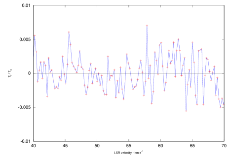
Figure 3: Baseline-subtracted line-to-continuum flux ratio around G34.3+0.1 for the 55 MHz OH line. The velocity resolution is 0.25 $km~{}s^{-1}$ per channel.

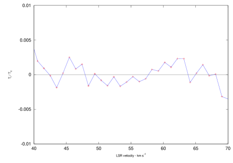
Figure 4: Baseline-subtracted line-to-continuum flux ratio around G34.3+0.1, smoothed to a velocity resolution of 1.0 $km~{}s^{-1}$ per channel.

The equation of radiative transfer gives

$$T_{l}=T_{bg}e^{-\tau_{\nu}}+T_{x}(1-e^{-{\tau}_{\nu}})$$

where $T_{bg}$ is the brightness temperature of the background source providing the radiation and $T_{x}$ is the excitation temperature.

Both the background temperature $T_{bg}$ and the excitation temperature $T_{x}$ contribute to the maser line brightness, but when $T_{bg}$ far exceeds $T_{x}$, say $T_{bg}>10|T_{x}|$, we can omit the contribution of $T_{x}$ to $T_{l}$. The 3$\sigma$ limit to the line brightness temperature from our observation is $T_{l}$ = 74 K for a 0.25 $km~{}s^{-1}$ channel which translates into 26.5 Jy. At a resolution of 1 $km~{}s^{-1}$, the limiting flux is 17.3 Jy. For comparison for the 53 MHz line, Menon et al. (2005) place a limit of 49 Jy at a velocity resolution of 4.6 $km~{}s^{-1}$.

For a maser that is $100\ mas$(Hoffman et al., 2003) in size, the beam dilution factor for the $10\degr$ GMRT beam is $1.3\times 10^{1\!1}$. Given $T_{bg}$ = 32100 K, we obtain the maser amplification, omitting the contribution from $T_{x}$, as

$$G=\frac{74\times 1.3\times 10^{1\!1}}{32100}\sim 3\times 10^{8}$$

providing an upper limit to the optical depth as $log(G)$ = 19.52. At a resolution of 1.0 $km~{}s^{-1}$, we get an upper limit of $\tau=log(G)-log(74/16.49)=18.58$ given that $T_{l}=16.49$ K. The calculation above assumes that (some reasonable fraction of) the Galactic synchrotron emission provides the background radiation that is amplified by the maser.

References

- Udaya Shankar et al. (2009) N. Udaya Shankar, K. S. Dwarakanath, S. Amiri, R. Somashekar, B. S. Girish, Wences Laus, Arvind Nayak, 2009, The Low Frequency Radio Universe, ASP Conf. Ser., 407, 393
- Claussen et al. (1997) Claussen M. J., Frail D. A., Goss W. M., Gaume R. A., 1997, ApJ, 489, 143
- Destombes et. al (1977) Destombes J. L., Marliere C., Baudry A., Brillet J., 1977, A&A, 60, 55
- Dwarakanath & Udaya Shankar (1990) Dwarakanath K. S., Udaya Shankar N., 1990, JApA, 11, 323
- Elitzur (1992) Elitzur M., 1992, Astronomical Masers, Kluwer Academic Press
- Frail et al. (1996) Frail D. A., Goss W. M., Reynoso E. M., Giacani E. B., Green A. J., Otrupcek R., 1996, AJ, 111, 1651
- Hoffman et al. (2003) Hoffman I. M., Goss W. M., Brogan C. L., Claussen M. J., Richards A. M. S., 2003, ApJ, 583, 272
- Kanekar et al. (2004) Kanekar N., Chengalur J. N., Ghosh T., 2004, PRL, 93, 5
- van Langevelde et al. (1995) van Langevelde H. J., van Dishoeck E. F., Sevenster M. N., Israel F. P., 1995, ApJ, 448, L123
- Menon et al. (2005) Menon S. M., Roshi D. A, Prasad T. R., 2005, MNRAS, 356, 958
- Roy et al. (2009) Roy J., Gupta Y., Ue-Li Pen, Peterson J. B., Kudale S., Kodilkar J., 2009, arXiv:0910.1517v1
- Turner (1979) Turner B.E., 1979, A&AS, 37