From Bijels to Pickering emulsions: a lattice Boltzmann study

Abstract

Particle stabilized emulsions are ubiquitous in the food and cosmetics industry, but our understanding of the influence of microscopic fluid-particle and particle-particle interactions on the macroscopic rheology is still limited. In this paper we present a simulation algorithm based on a multicomponent lattice Boltzmann model to describe the solvents combined with a molecular dynamics solver for the description of the solved particles. It is shown that the model allows a wide variation of fluid properties and arbitrary contact angles on the particle surfaces. We demonstrate its applicability by studying the transition from a “bicontinuous interfacially jammed emulsion gel” (bijel) to a “Pickering emulsion” in dependence on the contact angle, the particle concentration, and the ratio of the solvents.

I Introduction

Using particles in a manner similar to surfactants in order to stabilize emulsions is very attractive in particular for the food-, cosmetics-, and medical industry to stabilize, e.g. barbecue sauces and sun cremes or in order to produce sophisticated ways to deliver drugs at the right position in the human body. The microscopic processes leading to the commercial interest can be understood by assuming an oil-water mixture. Without any additives, phase separation would take place and the oil would float on top of the water. Adding small particles, however, causes these particles to diffuse to the interface which is being stabilized due to a reduced surface energy. If for example individual droplets of one phase are covered by particles, such systems are also referred to as “Pickering emulsions” and are known since the beginning of the last century bib:ramsden-1903 ; bib:pickering-1907 . Particularly interesting properties of such emulsions are the blocking of Ostwald ripening and the rheological properties due to irreversible particle adsorption at interfaces as well as interface bridging due to particle monolayers bib:arditty-whitby-binks-schmitt-leal-calderon ; bib:binks-clint-whitby-2005 ; bib:arditty-schmitt-giermanska-Kahn-leal-calderon ; bib:binks-horozov .

Recently, there has been a growing interest in particles suspended in multiphase or multicomponent flows bib:binks-horozov ; bib:binks-2002 ; bib:herzig-robert-zand-cipelletti-pusey-clegg ; bib:arditty-whitby-binks-schmitt-leal-calderon , which led to the discovery of a new material type, the “bicontinous interfacially jammed emulsion gel” (bijel) bib:cates-clegg-2008 . The existence of the bijel was predicted in 2005 by Stratford et al. bib:stratford-adhikari-pagonabarraga-desplat-cates-2005 ; bib:kim-stratford-adhikari-cates and experimentally confirmed by Herzig et al. in 2007 bib:herzig-white-schofield-poon-clegg . In contrast to Pickering emulsions which consist of unconnected particle stabilised droplets distributed in a second continuous fluid phase, the bijel shows an interface between two continuous fluid phases which is covered by particles.

Since the particles used for stabilization have a larger size than surfactant molecules and do not present any amphiphilic properties, concepts developed for the description of surfactant stabilized systems are often not applicable. Instead, theoretical models have to be developed and experiments have to be performed which consider the specific properties of particle-stabilized systems. These include the particle’s contact angle, the strong interparticle capillary forces, or the pH value and electrolyte concentration of the solvents bib:binks-horozov ; bib:binks-2002 ; bib:tcholakova-denkov-lips-2008 ; bib:aveyard-binks-clint ; bib:arditty-schmitt-giermanska-Kahn-leal-calderon . However, even today our quantitative understanding of solid stabilized emulsions is still far from satisfactory.

Computer simulations are promising to understand the dynamic properties of particle stabilized multiphase flows. However, the shortcomings of traditional simulation methods quickly become obvious: a suitable simulation algorithm is not only required to deal with simple fluid dynamics but has to be able to simulate several fluid species while also considering the motion of the particles and the fluid-particle interactions. Some recent approaches trying to solve these problems utilize the lattice Boltzmann method for the description of the solvents bib:succi-01 . The lattice Boltzmann method can be seen as an alternative to conventional Navier Stokes solvers and is well established in the literature. It is attractive for the current application since a number of multiphase and multicomponent models exist which are comparably straightforward to implement bib:shan-chen-93 ; bib:shan-doolen ; bib:shan-chen-liq-gas ; bib:swift-osborn-yeomans ; bib:swift-orlandini-osborn-yeomans ; bib:gunstensen-rothman-zaleski-zanetti ; bib:lishchuk-care-halliday-2003 . In addition, the method has been combined with a molecular dynamics algorithm to simulate arbitrarily shaped particles in flow and is commonly used to study the behavior of particle-laden single phase flows Ladd94a ; Ladd94b ; Ladd01 ; bib:jens-herrmann-bennaim:2008 .

A few groups combined multiphase lattice Boltzmann solvers with the known algorithms for suspended particles bib:stratford-adhikari-pagonabarraga-desplat-cates-2005 ; bib:joshi-sun . In this paper we follow an alternative approach: we present a method based on the multicomponent lattice Boltzmann model of Shan and Chen bib:shan-chen-93 which allows the simulation of multiple fluid components with surface tension. Our model generally allows arbitrary movements and rotations of arbitrarily shaped hard shell particles. It does not require fluid-filled particles and thus does not suffer from unphysical behavior caused by oscillations of the inner fluid bib:onishi-kawasaki-chen-ohashi . Further, it allows an arbitrary choice of the particle wettability – one of the most important parameters for the dynamics of multiphase suspensions bib:binks-horozov ; bib:binks-2002 .

The remainder of the paper is organised as follows: after a description of the Shan-Chen approach for multicomponent lattice Boltzmann simulations and an extension of the lattice Boltzmann method to simulate suspensions, a way to combine the two methods is proposed. The influence of the parameters of the model on the contact angle as a measure of wettability is studied in the following section. Then the suitability of the new method is tested by performing a detailed study of the formation of bijels and Pickering emulsions.

II The multicomponent lattice Boltzmann model

The dynamics of the fluid solvents is simulated by a multicomponent lattice Boltzmann model following the approach of Shan and Chen bib:shan-chen-93 . Here, each component follows a lattice Boltzmann equation

$$f_{i}^{c}\left(\mathbf{x}+\mathbf{c}_{i},t+1\right)=f_{i}^{c}\left(\mathbf{x},t\right)+\Omega_{i}^{c}(\mathbf{x},t),$$ (1)

where $f_{i}^{c}\left(\mathbf{x},t\right)$ is the single particle distribution function for component $c$ in the direction $\mathbf{c}_{i}$ ($i=1,\ldots,N$) at a discrete lattice position $\mathbf{x}$ and at timestep $t$. In this work we use exclusively the so-called D3Q19 implementation, where $N=19$ velocities are used on a three dimensional lattice. For simplicity, the length of a timestep and the lattice constant are set to 1, i.e. all units are given in lattice units if not stated otherwise. $\Omega_{i}^{c}$ is the Bhatnagar-Gross-Krook (BGK) collision operator bib:bgk ,

$$\Omega_{i}^{c}(\mathbf{x},t)=-\frac{f_{i}^{c}(\mathbf{x},t)-f_{i}^{\textnormal{eq}^{c}}\left(\rho^{c}(\mathbf{x},t),{\bf u}^{c}({\bf x},t)\right)}{\tau^{c}},$$ (2)

which is a relaxation towards the local equilibrium distribution function

$$\!f_{i}^{\textnormal{eq}^{c}}\!\!\!=\!\!\zeta_{i}\rho^{c}\!\left[\!1\!+\!\frac{{\bf c}_{i}{\bf u}}{c_{s}^{2}}\!+\!\frac{({\bf c}_{i}{\bf u})^{2}}{2c_{s}^{4}}\!-\!\frac{u^{2}}{2c_{s}^{2}}\!+\!\frac{({\bf c}_{i}{\bf u})^{3}}{6c_{s}^{6}}\!-\!\frac{u^{2}({\bf c}_{i}{\bf u})}{2c_{s}^{4}}\right]\!$$ (3)

on a time scale given by the relaxation time $\tau^{c}$ bib:chen-chen-martinez-matthaeus . Here, $\rho^{c}\left(\mathbf{x},t\right)=\rho_{0}\sum_{i}f^{c}_{i}\left(\mathbf{x},t\right)$ is the fluid density with reference density $\rho_{0}$ and ${\bf u}={\bf u}^{c}({\bf x},t)$ is the macroscopic bulk velocity of the fluid, given by $\rho^{c}({\bf x},t){\bf u}^{c}({\bf x},t)\equiv\sum_{i}f_{i}^{c}({\bf x},t){\bf c}_{i}$. $\zeta_{i}$ are the coefficients resulting from the velocity space discretization and $c_{s}=1/\sqrt{3}$ is the speed of sound, both of which are determined by the choice of the lattice. The kinematic viscosity of the fluid is given by $\nu^{c}=c_{s}^{2}(\tau^{c}-1/2)$.

The interaction between fluid components $c$ and $c^{\prime}$ is introduced as a self-consistently generated mean field force

$${\bf F}^{c}({\bf x},t)\equiv-\Psi^{c}({\bf x},t)\sum_{c^{\prime}}g_{cc^{\prime}}\sum_{\bf x^{\prime}}\Psi^{c^{\prime}}({\bf x^{\prime}},t)({\bf x^{\prime}}-{\bf x})\mbox{ ,}$$ (4)

where $\bf x^{\prime}$ are the nearest neighbors and $\Psi^{c}\left(\mathbf{x}\right)$ is the so-called effective mass, which can have a general form for modeling various types of fluids. We choose

$$\Psi^{c}\left(\mathbf{x},t\right)=\rho_{0}\left(1-\exp\left({-\frac{\rho^{c}\left(\mathbf{x},t\right)}{\rho_{0}}}\right)\right).$$ (5)

$g_{cc^{\prime}}$ is a force coupling constant whose magnitude controls the strength of the interaction between components $c$, $c^{\prime}$ and is set positive to mimic repulsion. The dynamical effect of the force is realized in the BGK collision operator by adding to the velocity ${\bf u}$ in the equilibrium distribution the increment

$$\Delta{\bf u}^{c}({\bf x},t)=\frac{\tau^{c}{\bf F}^{c}({\bf x},t)}{\rho^{c}({\bf x},t)}\mbox{ .}$$ (6)

The force also enters the calculation of the actual macroscopic bulk velocity as bib:guo-zheng-shi:2002 ; bib:jens-narvaez-zauner-raischel-hilfer:2010

$${\bf u}^{c}({\bf x},t)=\frac{\sum_{i}f_{i}^{c}\left({\bf x},t\right){\bf c}_{i}}{\rho^{c}\left({\bf x},t\right)}+\frac{1}{2}{\bf F}^{c}({\bf x},t).$$ (7)

In this paper two fluids with identical properties are used which are called “blue” (“b”) and “red” (“r”). To simplify statements about the fluid ratio at a certain position an order parameter

$$\phi\left(\mathbf{x},t\right)=\rho^{\textnormal{r}}\left(\mathbf{x},t\right)-\rho^{\textnormal{b}}\left(\mathbf{x},t\right)$$ (8)

is introduced. The Shan-Chen model is a diffuse interface method, where interfaces between different fluids are about four lattice sites wide. For the analysis below we define the interface position to be located where the order parameter vanishes.

III Suspended particles

Pioneering work on the development of an extension to the lattice Boltzmann method to incorporate particles has been done by Ladd et al. Ladd94a ; Ladd94b ; Ladd01 . The method has been applied to suspensions of spherical and non-spherical particles by various authors bib:jens-herrmann-bennaim:2008 ; bib:aidun-lu-ding ; bib:stratford-adhikari-pagonabarraga-desplat-cates-2005 ; bib:joshi-sun . Recently, the inclusion of Brownian motion was revisited and clarified in more detail bib:adhikari-stratford-cates-wagner-05 ; bib:duenweg-schiller-ladd:2007 . The suspended particles are assumed to be homogeneous spheres with radius $r_{\textnormal{par}}$. In our implementation of the method Newton’s equations for the momentum

$$\mathbf{F}=m\cdot\frac{\mathrm{d}\mathbf{u}_{\textnormal{par}}}{\mathrm{d}t}$$ (9)

and the angular momentum

$$\mathbf{D}=J\cdot\frac{\mathrm{d}\omega}{\mathrm{d}t}$$ (10)

are solved with a leap frog integrator to simulate their behavior. Here, $\mathbf{F}$ is the force acting on a particle, $m$ is its mass and $\mathbf{u}_{\textnormal{par}}$ its velocity. $\mathbf{D}$ is the torque, $J$ the moment of inertia and $\omega$ the angular velocity.

The particles are discretized on the lattice and interactions between the fluid and the particles are introduced by marking all lattice sites that are inside the particle as solid nodes for the fluid, at which bounce back boundary conditions are applied Ladd01 . Bounce back boundary conditions reflect the incoming distributions at a site back to where they came from, so that the streaming step is modified to

$$f_{i}^{c}\left(\mathbf{x},t+1\right)=f_{i}^{c}\left(\mathbf{x}-\mathbf{c}_{i},t\right),$$ (11)

for all $i$ where $\mathbf{x}-\mathbf{c}_{i}$ is not a solid node to

$$f_{i}^{c}\left(\mathbf{x},t+1\right)=f_{i^{\prime}}^{c}\left(\mathbf{x},t\right),$$ (12)

for all $i$ where $\mathbf{x}-\mathbf{c}_{i}$ is a solid node. Here, $i^{\prime}$ is defined as the index corresponding to $\mathbf{c}_{i}=-\mathbf{c}_{i^{\prime}}$. This results in a no-slip boundary located halfway between the fluid and the solid node. The change of momentum of the fluid that is reflected at the boundary has to be compensated by a momentum change of the particle itself as given by

$$\Delta\mathbf{p}(t)=2\cdot\rho^{c}(\mathbf{x},t)\mathbf{c}_{i}.$$ (13)

As we assume the length of a time step $\mathrm{d}t$ to be $1$ this corresponds to a force

$$\mathbf{F}(t)=2\cdot\rho^{c}(\mathbf{x},t)\mathbf{c}_{i}$$ (14)

and a torque

$$\mathbf{D}(t)=\mathbf{F}(t)\times\mathbf{r}(t),$$ (15)

on the particle. Here, $\mathbf{r}(t)$ is the vector pointing from the center of the particle to the site of the reflection. Since the particles are not stationary but move over the lattice, the bounce back rule does not correctly reproduce the velocity of the reflected fluid. It is therefore corrected as

$$f_{i}^{c}\left(\mathbf{x},t+1\right)=f_{i^{\prime}}^{c}\left(\mathbf{x},t\right)-\frac{1}{6}\rho^{c}\left(\mathbf{x},t\right)\mathbf{u}_{\textnormal{surf}}\left(\mathbf{x},t\right)\cdot\mathbf{c}_{i^{\prime}},$$ (16)

where $\mathbf{u}_{\textnormal{surf}}(\mathbf{x},t)$ is the velocity of the particle surface on which the fluid is reflected. This effect also leads to a change in transfered momentum, so that the force acting on the particle is

$$\mathbf{F}(t)=\left(2\rho^{c}(\mathbf{x},t)-\frac{1}{6}\rho^{c}(\mathbf{x},t)\mathbf{u}_{\textnormal{surf}}(\mathbf{x},t)\cdot\mathbf{c}_{i^{\prime}}\right)\mathbf{c}_{i^{\prime}}.$$ (17)

When the particle moves over the lattice, individual lattice sites can be either occupied by it in front of the particle or be released at its back. In case of newly occupied sites, the fluid on the site is deleted and its momentum transfered to the particle by adding

$$\mathbf{F}(t)=-\rho^{c}(\mathbf{x},t)\mathbf{u}^{c}(\mathbf{x},t).$$ (18)

In case of the particle vacating a lattice site new fluid is created with the initial fluid density and the velocity of the particle surface $\mathbf{u}_{\textnormal{surf}}(\mathbf{x},t)$ at the corresponding site:

$$f_{i}^{c}(\mathbf{x},t)=\rho^{c}_{\textnormal{init}}\cdot f_{i}^{\textnormal{eq}^{c}}\left(\mathbf{u}_{\textnormal{surf}}(\mathbf{x},t),\rho(\mathbf{x},t)\right).$$ (19)

To satisfy conservation of momentum this again leads to a force on the particle,

$$\mathbf{F}(t)=\rho^{c}_{\textnormal{init}}\mathbf{u}_{\textnormal{surf}}(\mathbf{x},t).$$ (20)

Interactions between particles can be taken into account similar to standard molecular dynamics implementations. In the current paper, we only consider Hertzian contact forces to mimic hard spheres and a lubrication correction to correct for the limitations of the lattice Boltzmann method to describe the hydrodynamics properly on scales below the lattice resolution. When particles collide the resulting forces are derived from the Hertzian potential bib:hertz

$$V_{\rm Hertz}\left(r\right)=\begin{cases}K_{\textnormal{Hertz}}\cdot\left(2r_{\textnormal{par}}-r\right)^{\frac{5}{2}}&\mbox{for }r<2r_{\textnormal{par}}\\ 0&\mbox{else,}\\ \end{cases}$$ (21)

with $K_{\textnormal{Hertz}}$ being a constant bib:jens-hecht-ihle-herrmann:2005 . When two particles move towards each other the lubrication interaction between them results in a force separating the particles. If there is not at least one lattice site between the particles to resolve the flow, this force is not properly reproduced by the simulation and a lubrication correction has to be added as given by

$$\mathbf{F}_{\textnormal{lub}}=-\frac{6\pi\nu^{c}r_{\textnormal{par}}^{4}}{\left(2r_{\textnormal{par}}\right)^{2}}\frac{\mathbf{r}}{\left|\mathbf{r}\right|}\left[\frac{\mathbf{r}}{\left|\mathbf{r}\right|}\left(\mathbf{u}_{1}-\mathbf{u}_{2}\right)\right]\left(\frac{1}{\left|\mathbf{r}\right|-2r_{\textnormal{par}}}-1\right),$$ (22)

where $\mathbf{r}$ is the vector connecting the particle centers and $\mathbf{u}_{1,2}$ is their respective velocity Ladd01 ; Hecht07 . It is introduced at particle distances smaller than $\frac{2}{3}$ lattice units and limited to it’s value at a distance of $\frac{1}{10}$ of a lattice unit to avoid numerical instabilities due to the divergence at $\left|\mathbf{r}\right|=2r_{\textnormal{par}}$.

IV Particles in multicomponent fluids

In order to develop a simulation algorithm for particles in multicomponent flows the previously described methods can be combined as described in the current section. First, when extending the coupling between particles and fluid to multiple components the treatment of lattice sites that are uncovered by the moving particle has to be adapted. In the original algorithm for a single fluid, such sites are filled with the initial fluid density $\rho^{c}_{\rm init}$. However, re-initializing such sites with multiple fluid components can lead to artefacts since it is not a priori the case that the correct fluid composition should correspond to the initial state of the simulation. For example, one kind of fluid could appear in a region where only the other fluid is present. To prevent such artefacts we use the average surrounding fluid density

$$\bar{\rho}^{c}(\mathbf{x},t)=\frac{1}{N_{\textnormal{NP}}}\sum_{i_{\textnormal{NP}}}\rho^{c}(\mathbf{x}+\mathbf{c}_{i_{\textnormal{NP}}},t),$$ (23)

where $i_{\textnormal{NP}}$ are all indices $i$ for which $\mathbf{x}+\mathbf{c}_{i}$ is a non-particle site. $N_{\textnormal{NP}}$ is the number of these sites. Similar to the method described in bib:aidun-lu-ding ; bib:lorenz-caiazzo-hoekstra , the uncovered sites are re-initialized with

$$\rho_{\textnormal{new}}^{c}(\mathbf{x},t)=\bar{\rho}^{c}(\mathbf{x},t)$$ (24)

following a similar approach as in Eqs. 19 and 20, i.e.

$$f_{i}^{c}(\mathbf{x},t)=\rho_{\textnormal{new}}^{c}(\mathbf{x},t)\cdot f_{i}^{\textnormal{eq}}\left(\rho_{\textnormal{new}}^{c}(\mathbf{x},t),\mathbf{u}_{\textnormal{surf}}(t)\right)$$ (25)

and

$$\mathbf{F}=\sum_{c}\rho_{\textnormal{new}}^{c}(\mathbf{x},t)\mathbf{u}_{\textnormal{surf}}(t).$$ (26)

The second modification of the original algorithms is required to correctly take into account the effect of the fluid-fluid interaction forces on the fluid in the direct vicinity of a particle. For the calculation of the forces between different fluid components, also the empty lattice sites inside a particle are considered if one follows Eq. 4. Since there are no Shan-Chen forces acting in the direction from the particle to the fluid, the fluid forms a layer of increased density around the particle. To avoid this artefact, the outermost layer of lattice sites inside the particle is not kept empty, but is filled with a virtual fluid density which is equivalent to the average of the surrounding densities $\bar{\rho}$:

$$\rho^{c}(\mathbf{x},t)=\bar{\rho}^{c}(\mathbf{x},t)$$ (27)

This virtual fluid inside the particles does not follow the lattice Boltzmann equation, i.e. the advection and collision steps are not applied.

Further, the Shan-Chen like force acting from the fluid surrounding a particle on the particle itself has to be accounted for. This is implemented by summing up all Shan-Chen forces

$${\bf F}(t)=\sum_{{\bf x}}\sum_{c}{\bf F}^{c}({\bf x},t)$$ (28)

acting on every lattice site ${\bf x}$ inside the particle. This force and the corresponding torque are then added to the particle within the molecular dynamics algorithm. The forces on the fluid outside the particles are calculated as before with the virtual fluid being treated like a regular fluid in the Shan-Chen force computation. This leads to a balanced force on the fluid sites near the particle surface and therefore prevents the formation of a layer of increased density. This is demonstrated in Fig. 1, where the left subfigure shows a particle with $r_{\textnormal{par}}=10$ being filled with virtual fluid while in the right subfigure the particle is not filled with a virtual fluid. The particle is set at an interface created by two lamellae of red and blue fluids at the center of the shown area. Periodic boundary conditions are applied causing a second interface to appear at the left and right borders of the sketches. As we use a diffuse interface method for the fluids, the interfaces cover about four lattice sites depicted by the varying grey scale. Without the virtual fluid, the halo of increased density can clearly be seen, while adding the virtual fluid successfully allows to correct for this inconsistency.

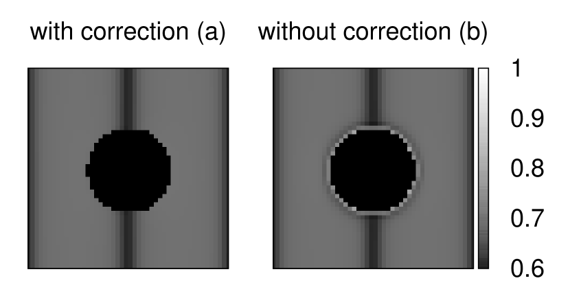
Figure 1: $\sum_{c}\rho^{c}$ after 2000 timesteps in the presence of a particle with $r_{\textnormal{par}}=10$ at an interface at the center of the shown area. The cut on the left (a) shows a particle being filled with virtual fluid, while on the right (b) the particle is empty as in the original algorithm. Without the virtual fluid, the halo of increased density can clearly be seen, while adding the virtual fluid successfully allows to correct for this inconsistency. The parameters of the simulation were $\rho_{0}=1$ and $\tau=1$ for both species, the system of size $48^{3}$ lattice sites was initially divided into two lamellae of width 24 lattice sites with density $\rho^{\textnormal{r}}=\rho^{\textnormal{b}}=0.7$, respectively. All units are given in lattice units throughout this paper.

The advantage of a virtual fluid inside the particles is that it can be utilized to modify the wettability of the particles. Here, we follow an approach which has been introduced to model hydrophobic fluid-surface interactions for studying flow in hydrophobic microchannels or droplets on surfaces with arbitrary contact angles bib:jens-kunert-herrmann:2005 ; bib:jens-kunert:2008c ; bib:jens-jari:2008 ; bib:jens-schmieschek:2010 . Our approach is equivalent to the method presented in bib:onishi-kawasaki-chen-ohashi . The Shan-Chen interaction between the particles and the fluids can be modified by tuning the density of the local virtual fluids. Increasing one of them by an amount $\left|\Delta\rho\right|$ causes the particle surface to “prefer” this fluid with respect to the other one, i.e. the repulsion between the increased component and the unmodified one increases. $\Delta\rho$ is called “particle color” and a positive particle color is defined as an addition of “red” fluid, i.e.

$$\rho_{\rm new}^{\rm r}=\bar{\rho}^{\rm r}+\left|\Delta\rho\right|,$$ (29)

whereas a negative color corresponds to “blue” fluid being added, i.e.

$$\rho_{\rm new}^{\rm b}=\bar{\rho}^{\rm b}+\left|\Delta\rho\right|.$$ (30)

In the next section we demonstrate that the particle color can be used to tune the contact angle of the particle surface at an interface in order to resemble specific fluids and solid materials. As an alternative to the virtual fluid, a modified version of Eq. 4 that takes solid lattice sites and fluid-surface interactions into account could be developed, but the approach presented here is simpler to implement and does not have any relevant impact on the performance of the code.

The changing discretization of the particle together with the fluid-surface interaction force leads to slight mass errors during the step in which vacated lattice nodes are refilled with fluid. This effect is especially strong for small particles and high forces (large values for $g_{\textnormal{cc'}}$). Typical test cases have shown that the total mass after very long simulation times ($10^{7}$ timesteps) increases by about one percent. This can be explained by the simple interpolation for the amount of newly created fluid which is necessary since no analytical solution for the multicomponent Shan-Chen model is known that describes the density profile at interfaces. Even though the effect is very small, it can be suppressed if newly created fluid densities $\rho_{\textnormal{new}}^{c}$ are scaled with a correction factor which depends on the total mass error $\Delta\rho^{c}$ up to the current timestep and the total number of lattice sites in the system $N$. This leads to a modification of Eq. 24:

$$\rho_{\textnormal{new}}^{c}=\bar{\rho}^{c}\left(1-C_{0}\frac{\sum_{c}\rho_{\textnormal{init}}^{c}}{\rho_{\textnormal{init}}^{c}}\frac{\Delta\rho^{c}}{N}\right).$$ (31)

The rate of the adaptive correction can be tuned with the parameter $C_{0}$. Due to the very small mass error, the correction can act very slowly, but should not be chosen too fast in order to avoid hysteresis effects. Further, Eq. 31 reduces unphysical density gradients at particle surfaces and thus contributes to the stability of the algorithm. Repeating the same test case as above with a correction factor of $C_{0}=10$ results in a deviation of the mass of 0.03 percent after $10^{7}$ timesteps.

V Contact angle measurements

The contact angle $\theta$ is a common measure for the wettability of the particle by the two fluid components. The influence of various simulation parameters on the contact angle is investigated in the current section.

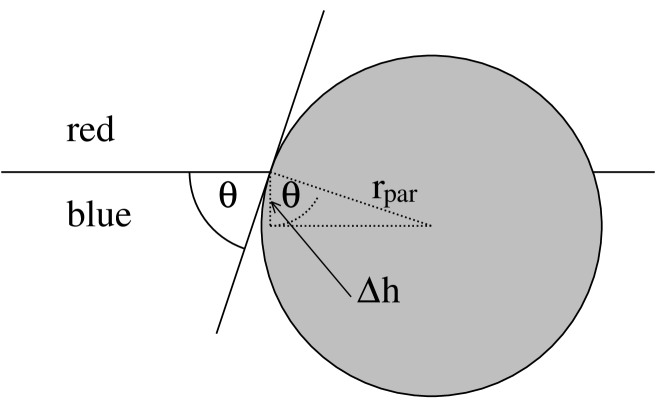
Figure 2: Definition of the contact angle $\theta$ for a particle of radius $r_{\textnormal{par}}$ at the interface between the two fluid components. $\Delta h$ is the distance from the particle center to the interface.

In order to measure the contact angle the following setup is used in the simulations: in $z$ direction, one half of the lattice is filled with one fluid component, the other half with the second one. The particle is placed at the interface at $t=0$ and the simulation is started. The interface between the two components is tracked via the (linearly interpolated) position at which the order parameter is zero. Then, the contact angle $\theta$ can be calculated by

$$\cos\left(\theta\right)=\frac{\Delta h}{r_{\textnormal{par}}},$$ (32)

where $\Delta h$ is the difference between the interface position and the particle center in the direction perpendicular to the interface (cf. figure 2).

Figure 3: Contact angle versus time for a 48x48x256 system with particle color 0.02, $r_{\textnormal{par}}=10$, $g_{\textnormal{br}}=0.08$, and fluid density $\rho_{\textnormal{init}}=0.6$. After a rapid change from about $93^{\circ}$ to about $107^{\circ}$ the contact angle stays at a constant value and only shows small oscillations with an amplitude of about $1^{\circ}$.

To study the time-evolution of the contact angle a system of size 48x48x256 lattice sites is used. The particle has a radius of 10 lattice sites and a color of 0.02. The initial fluid density is 0.6 and $g_{\textnormal{br}}=0.08$. Figure 3 shows the time dependence of the contact angle. After a short, fast movement at the beginning of the simulation the contact angle oscillates slightly around a fixed value. Here and for all further graphs in this section, we average the contact angle over the timesteps from $6\cdot 10^{5}$ to $9\cdot 10^{5}$ leading to a final value of $\theta=\left(107.03\pm 0.26\right)^{\circ}$. The error is given by the standard deviation of the data. Relating the variation of the angle to a change of the position of the interface on the lattice with regards to the particle center results in $\Delta h=\left(-2.93\pm 0.04\right)$ lattice units. The error in the position measurement is very small with respect to the lattice resolution.

Figure 4a shows the resulting contact angle for different particle sizes between $r_{\textnormal{par}}=2$ and $r_{\textnormal{par}}=16$. For small particle radii the error increases substantially and the measured angle is not equivalent to the one measured for larger particles, but is up to $15^{\circ}$ larger. For example, for $r_{\textnormal{par}}=2$ the contact angle is $\left(120.9\pm 6.0\right)^{\circ}$. For particles larger than $r_{\textnormal{par}}=5$ the error stays below $1.5^{\circ}$ and the measured angles are in the range of $106$ to $110^{\circ}$. Smaller particles are more susceptible to small forces because of their smaller mass, also one has to keep in mind that our lattice Boltzmann multicomponent model is a diffuse interface method. Since the interface is about four lattice sites wide, small particles are completely inside the interface region. For particles with a non-integer radius the error and the angle are larger than for particles with integer radii. This can be adhered to being a discretisation effect as the particles move on the lattice.

Figure 4: a) Contact angle versus particle size. The system size is 48x48x256, the particle color 0.02, $g_{\textnormal{br}}=0.08$, and $\rho_{\textnormal{init}}=0.6$. The average measured angle and errors given by the standard deviation over timesteps from $6\cdot 10^{5}$ to $9\cdot 10^{5}$ are shown. The contact angle for $r_{\textnormal{par}}=2$ is $\left(120.9\pm 6.0\right)^{\circ}$, for particles larger than $r_{\textnormal{par}}=5$ the error stays below $1.5^{\circ}$ and the angles are in the range of $106^{\circ}$ to $110^{\circ}$. Particles with a non-integer radius show larger contact angles, which can be adhered to a discretization effect.
b) Contact angle versus particle color for $\rho_{\textnormal{init}}=0.7$. The data can be fitted with the equation $\theta=442\cdot\Delta\rho+90$ (dashed line).

The dependency of the contact angle $\theta$ on the particle color $\Delta\rho$ is shown in Fig. 4b. One can see an almost linear relation between the contact angle and the particle color in the range from a color of $\Delta\rho=-0.125$ (contact angle $33.2^{\circ}$) to $\Delta\rho=0.125$ (contact angle $147.6^{\circ}$). Included in the figure is a linear fit given by $\theta=442\cdot\Delta\rho+90$ to stress this linear behavior. The simulations with a particle color of $\Delta\rho\geq 0.15$ and $\Delta\rho\leq-0.15$ result in a detachment of the particle from the interface. Thus, it is possible to choose a specific particle color to obtain the related contact angle or to force detachment from one of the fluids.

As a next step we investigate the influence of the strength of the fluid-fluid interaction force on the contact angle. For strong forces determined by large $g_{\textnormal{br}}$ the interface is well defined and the surface tension high. Low $g_{\textnormal{br}}$ cause a low surface tension and thus a more diffuse interface. When the coupling constant $g_{\textnormal{br}}$ is varied, the contact angle $\theta$ changes as shown in Fig. 5a. The stronger the force the stronger the particle is kept at the interface. If the force is too weak the particle cannot be held at the interface anymore. For $g_{\textnormal{br}}\geq 0.1$ almost no change to the contact angle can be observed and $\theta$ converges to $93.0^{\circ}$ with an error smaller than $0.1^{\circ}$. For $g_{\textnormal{br}}\leq 0.08$ the contact angle increases dramatically until the particle does not stay attached to the interface at $g_{\textnormal{br}}\leq 0.07$. On the one hand, a well defined contact angle and well defined interfaces are preferrable requiring large values of $g_{\textnormal{br}}$. On the other hand, too large values can cause very high local flow velocities and the lattice Boltzmann method can become unstable. Thus, $g_{\textnormal{br}}$ should be chosen as small as possible.

Figure 5: a) Contact angle versus $g_{\textnormal{br}}$. For $g_{\textnormal{br}}\geq 0.1$ a contact angle of $93.0^{\circ}$ with an error smaller than $0.1^{\circ}$ is measured. The contact angle increases from this value at $g_{\textnormal{br}}=0.1$ to $98.0^{\circ}$ at $g_{\textnormal{br}}=0.08$ with an error below one degree. $g_{\textnormal{br}}=0.075$ results in a contact angle of $\left(113.6\pm 0.3\right)^{\circ}$ and for smaller $g_{\textnormal{br}}$ the particle detaches from the interface.
b) Contact angle versus the initial fluid density $\rho_{\textnormal{init}}$. $\rho_{\textnormal{init}}=0.9$ results in a contact angle of $92.5^{\circ}$. Reducing $\rho_{\textnormal{init}}$ causes the contact angle to decrease to $108.4^{\circ}$ at $\rho_{\textnormal{init}}=0.55$.

As can be observed in Fig. 5b, a variation of the initial fluid density $\rho_{\textnormal{init}}$ has a similar effect as a modification of the coupling constant on the contact angle. However, $\theta$ only changes from $108.5^{\circ}$ ($\rho_{\textnormal{init}}=0.55$) to $92.5^{\circ}$ ($\rho_{\textnormal{init}}=0.9$), i.e. the effect is much weaker. The reason for the lower impact on $\theta$ is given by our particular choice of the effective mass $\Psi^{c}\left(\mathbf{x}\right)$ (see Eq. 5) which causes a damping of the interactions for large densities.

The knowledge of the contact angle and particle shape together with a measurement of the surface tension between both fluids allows to measure the energy required to detach a trapped particle from an interface bib:binks-horozov . While for spherical particles it is straightforward to compute the detachment energy analytically, for highly anisotropic or complex shaped particles this is not easily possible. A simulation study based on the model proposed in this paper would allow a well founded understanding of the dependence of detachment energies on particle properties and could be compared to experimental data.

VI Bijel formation

The formation of a “bijel” (bicontinuous interfacially jammed emulsion gel) was first predicted by Stratford et. al. in 2005 bib:stratford-adhikari-pagonabarraga-desplat-cates-2005 . As stated in the introduction, bijels can form when (colloidal) particles are added to a mixture of two immiscible fluids. During the phase separation of the two fluids, the particles accumulate at the interface until those are fully jammed. Since the simulations performed by Stratford et. al. utilize a free energy based multiphase lattice Boltzmann model, we show in this section that the multicomponent model introduced in this paper is also able to model the formation of a bijel. We study the temporal development of the system and compare our results with the results of Stratford et al.. Further, we investigate the influence of the particle concentration, $g_{\textnormal{br}}$, and $\rho_{\textnormal{init}}=\sum_{c}\rho_{\textnormal{init}}^{c}$ on the bijel formation. The initial conditions for the simulations are as follows: an identical amount of the two fluid species is distributed randomly throughout the system. The initial positions of the colorless particles ($\theta=90^{\circ}$) are also chosen at random. In order to keep the system size at manageable $256^{3}$ lattice units and to be able to simulate a significant number of particles, the particle radius is kept at $r_{\textnormal{par}}=5$ lattice units in all simulations.

The conversion from lattice units to SI units of a system containing two identical fluids with the speed of sound ($c_{s}=1482.35$m/s) and kinematic visosity ($\nu=1.004\cdot 10^{-6}$m²/s) of water at 20^∘C results in a timestep of $\Delta t=9.14\cdot 10^{-13}$s and a lattice constant of $\Delta x=2.35$nm. Since we set our particle diameter to 10 lattice units, the physical diameter would be $23.5$nm and the side length of a cubic simulation volume with $256$ lattice units corresponds to $601.6$nm. The systems presented in this section are simulated for $2.8\cdot 10^{5}$ timesteps corresponding to $2.56\cdot 10^{-7}\textnormal{s}$.

Figure 6: Average domain size for a system with $g_{\textnormal{br}}=0.08$, $\rho_{\textnormal{init}}=0.7$ and a particle concentration of 20%. During the first $2.5\cdot 10^{4}$ steps of the simulation the average domain size grows from below 5 to its final value of about 31 lattice units.

As already stated correctly by Stratford et al., thermal fluctuations have only little effect on the phase separation and bijel formation and can thus be ignored in the simulations bib:stratford-adhikari-pagonabarraga-desplat-cates-2005 .

To analyze the development of structures in the simulated systems, we define the averaged time dependent lateral domain size $L(t)$ which consists of an average of its components $L_{i}$ along direction $i=x,y,z$ as given by

$$L_{i}(t)\equiv\frac{2\pi}{\sqrt{\left<k^{2}_{i}(t)\right>}}.$$ (33)

Here,

$$\left<k^{2}_{i}(t)\right>\equiv\frac{\sum_{\mathbf{k}}k_{i}^{2}S(\mathbf{k},t)}{\sum_{\mathbf{k}}S(\mathbf{k},t)}$$ (34)

is the second order moment of the three-dimensional structure function

$$S(\mathbf{k},t)\equiv\frac{1}{N}\left|\phi^{\prime}_{\mathbf{k}}(t)\right|^{2}$$ (35)

with respect to the Cartesian component $i$, $\left<\right>$ denotes the average in Fourier space, weighted by $S(\mathbf{k},t)$ and $N$ is the number of nodes of the lattice, $\phi^{\prime}_{\mathbf{k}}(t)$ the Fourier transform of the fluctuations of the order parameter $\phi^{\prime}\equiv\phi-\left<\phi\right>$, and $k_{i}$ is the $i$th component of the wave vector bib:jens-giupponi-coveney:2007 . The simulations are performed using a $256^{3}$ lattice, a coupling constant of $g_{\textnormal{br}}=0.08$, an initial fluid density of $\rho_{\textnormal{init}}=0.7$, a particle volume ratio $\alpha$ of 20 percent (about 6400 particles), a particle size of $r_{\textnormal{par}}=5$ lattice units, and a particle density of 1, i.e. the particles are slightly heavier than the fluid. The time development of the average domain size $L(t)$ is shown in Fig. 6. The figure clearly shows that the system comes to arrest after a brief period of phase separation. During the first $2.5\cdot 10^{4}$ timesteps the average domain size $L(t)$ increases from 5 lattice units to about 31 lattice units and stays at that value until the end of the simulation at $t=2.8\cdot 10^{5}$ timesteps. This qualitatively agrees to the results obtained by Stratford et al. bib:stratford-adhikari-pagonabarraga-desplat-cates-2005 . However, their simulation does not converge to a fixed domain size, which might be caused by the thermal motion incorporated in their model. While thermal fluctuations are not strong enough to detach the particles from the interface they might cause some local reordering of the particles and therefore support further domain growth. This effect would be favored by the small particle diameter used in the simulations presented in bib:stratford-adhikari-pagonabarraga-desplat-cates-2005 since the particle size is of the same order or even smaller than the interface thickness.

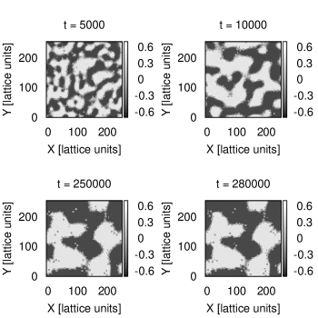
Figure 7: 2D cut of the order parameter $\phi$ at $z=0$ through the system studied in Fig. 6. The spots where $\phi=0$ correspond to the regions occupied by particles. $\phi$ shows pronounced differences between $t=5000$ and $t=10000$, while at timesteps $2.5\cdot 10^{5}$ and $2.8\cdot 10^{5}$ only minor rearrangements can be observed.

The arrest of the phase separation process can also be observed by visualizing a 2D cut at $z=0$ of the order parameter as in Fig. 7 or a 3D visualisation of $\phi$ as in Fig. 8. The differences between timesteps $t=5000$ and $t=10000$ are large while the system barely changes between timesteps $2.5\cdot 10^{5}$ and $2.8\cdot 10^{5}$. Both visualisations clearly demonstrate the bicontinuouity of the fluid domains. In particular Fig. 8 depicts how the particles get trapped at the fluid-fluid interface and cause the demixing process to stop.

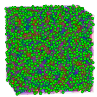
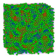
$t=5000$	$t=10000$
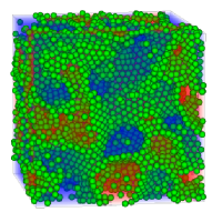
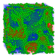
$t=250000$	$t=280000$

Figure 8: (Color online) 3D visualisation of the system presented in Figs. 6 and 7. Shown are the particles (in green/light gray) and the two fluids (in red/medium gray and blue/dark gray, respectively). The visualizations for $t=2.5\cdot 10^{5}$ and $t=2.8\cdot 10^{5}$ nicely depict the bicontinuouity of the fluids and the attachment of the particles to the interface.

Modifying the strength of the fluid-fluid interaction force by varying the coupling constant $g_{\textnormal{br}}$ also influences the resulting domain size. This is demonstrated in Fig. 9a, where the averaged lateral domain size $L$ is shown after $t=2.8\cdot 10^{5}$ timesteps and for different $g_{\textnormal{br}}$. While $g_{\textnormal{br}}=0.07$ leads to a domain size of about 33.7 lattice units, $g_{\textnormal{br}}=0.125$ results in an average size of 28 lattice units. The differences between the spatial directions at a certain $g_{\textnormal{br}}$ are below 0.5 lattice units. A higher value of the coupling constant leads to stronger forces attaching the particles to the interface. Therefore, the size of the interface increases because the particles cannot slightly shift away from it in order to accomodate more particles on the same interfacial area. As the number of particles in the system is kept constant, the interfacial area has to increase and therefore the resulting domains become smaller.

Figure 9: a) Average domain size versus $g_{\textnormal{br}}$ at $t=2.8\cdot 10^{5}$. With increasing $g_{\textnormal{br}}$ $L$ decreases from 33.7 lattice units at $g_{\textnormal{br}}=0.07$ to 28 lattice units at $g_{\textnormal{br}}=0.125$.
b) Average domain size versus $\rho_{\textnormal{init}}$. $\rho_{\textnormal{init}}=0.6$ leads to a $L$=32 lattice units. A larger value of $\rho_{\textnormal{init}}=0.9$ reduces $L$ to a value slightly below 30 lattice units. Error bars are given by the maximum deviation of $L_{x}$, $L_{y}$, $L_{z}$ from the mean.

For a variation of the initial bulk density $\rho_{\textnormal{init}}$ the arguments of the previous paragraph still hold. A larger value of $\rho_{\textnormal{init}}$ leads to stronger interaction forces and therefore to smaller structures as described above. While the coupling constant $g_{\textnormal{br}}$ directly changes the strength of the force $\rho_{\textnormal{init}}$ affects the force only indirectly through the effective mass which causes the effect to be less pronounced. As depicted in Fig. 9b the average domain size $L$ decreases from about 32 lattice units for $\rho_{\textnormal{init}}=0.6$ to below 30 lattice units for $\rho_{\textnormal{init}}=0.9$.

The connection between the area of the interface covered by particles and the size of the resulting structures can be best shown by varying the particle concentration $\alpha$. This is depicted in Fig. 10.

Figure 10: Average domain size versus particle concentration $\alpha$. Decreasing $\alpha$ from 0.35 to 0.15 leads to an increase of $L$ from 21.5 lattice units to 36 lattice units. If the concentration is further reduced to 0.05, finite size effects start to occur. Also shown is $L=\frac{3.86}{\alpha}+10.85$, the result of a fit to the concentration values between 0.15 and 0.35. Error bars are given by the maximum deviation of $L_{x}$, $L_{y}$, $L_{z}$ from the mean.

Increasing particle concentration leads to a larger interfacial area and therefore to finer structures. While the average domain size of a system with a particle concentration of 0.15 is about 36 lattice units this value decreases to about 22 lattice units for a concentration of 0.35. A too low particle concentration leads to such a small stabilized surface that finite size effects start to appear as they are well known from lattice Boltzmann simulations of spinodal decomposition bib:jens-giupponi-coveney:2007 . This can be seen for a concentration of 5%. Here, the structure size increases drastically, also the average domain size is not the same for all spatial directions anymore and varies by about 3 lattice units. It is possible to fit a function of the form $L={a}/{\alpha+b}$ with $a=3.85936$ and $b=10.8479$ to the values where finite size effect do not play a role.

VII Pickering emulsions

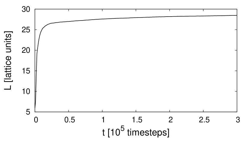
Figure 11: Average domain size over time for a system of size $256^{3}$, $g_{\textnormal{br}}=0.09$, $\rho_{\textnormal{init}}=0.66$, fluid ratio 1:3, particle color $-0.01$ and particle concentration $\alpha=0.15$. After a rapid growth of the domain size to over 25 lattice units during the first 25000 timesteps the domain size increases only slowly to slightly over 27 lattice units at timestep $3.0\cdot 10^{5}$.

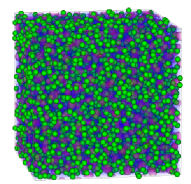
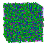
$t=5000$	$t=10000$
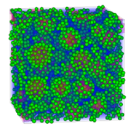
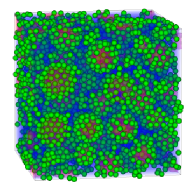
$t=250000$	$t=300000$

Figure 12: (Color online) 3D visualisation of the system described in Fig. 11. The particles (green/light gray) and the fluids (red/medium gray and blue/dark grey) are shown. The particles are attached to the interface between the fluid components and the red fluid forms spherical droplets inside the continuous blue fluid. While the change from timesteps 5000 to 10000 is significant the droplet growth is almost at rest between $t=2.5\cdot 10^{5}$ and $t=3.0\cdot 10^{5}$.

Another well known phenomenon that can be observed in mixtures of immiscible fluids and particles are Pickering emulsions bib:ramsden-1903 ; bib:pickering-1907 . Here, the particles are not necessarily equally wettable by the fluids anymore. Also, the ratio of the amount of fluid of different species deviates from 1. The result is a system where one phase is continuous while the other forms droplets which are stabilized by the particles. The particles prevent the droplets from merging when they collide and therefore stop the growth of the average droplet size. As before the droplet size can be measured utilizing $L(t)$ as shown in Fig. 11. Here, the lattice is $256^{3}$, the interaction constant $g_{\textnormal{br}}=0.09$, and the initial fluid density $\rho_{\textnormal{init}}=0.66$. The fluid ratio is 1:3 and the particles with a color of $\Delta\phi=-0.01$ have a volume concentration of 15%. As for the previously presented “bijels” a rapid growth of $L(t)$ from 5 to over 25 lattice units can be observed during the first 25000 timesteps of the simulation. The domain growth slows down to a slight decelerating growth afterwards. This agrees qualitatively with experimental results by Arditty et al. bib:arditty-whitby-binks-schmitt-leal-calderon .

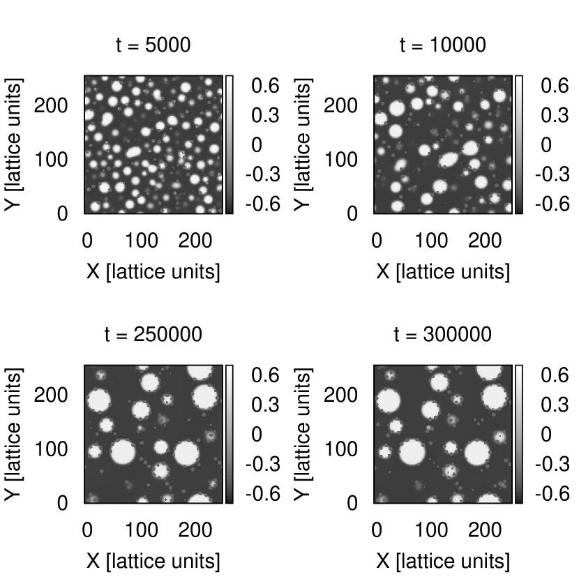
Figure 13: 2D cut at $z=0$ through the system described in figure 11 at different times. Shown is the order parameter $\phi$.

A three-dimensional visualisation of the order parameter $\phi$ and the particles is shown in Fig. 12 and accompanied by a two dimensional cut of the system at $z=0$ in Fig. 13. The particle covered droplets as well as the slowing down of droplet growth can be observed. While the system changes dramatically between timesteps 5000 and 10000 almost no difference can be observed when comparing step $2.5\cdot 10^{5}$ to step $3.0\cdot 10^{5}$.

Figure 14: Average domain size after $1\cdot 10^{6}$ timesteps versus particle concentration $\alpha$. System size $256^{3}$, $g_{\textnormal{br}}=0.08$, $\rho_{\textnormal{init}}=0.7$, fluid ratio 1:3 and particle color $-0.01$. Increasing $\alpha$ leads to a decreasing average domain size. Also shown is a fit with equation $\frac{2.12}{\alpha}+18.91$. Error bars are given by the maximum deviation of $L_{x}$, $L_{y}$, $L_{z}$ from the mean.

The influence of the interfacial area on the droplet size can be demonstrated by modifying the particle concentration. The resulting average domain size for different concentrations is shown in Fig. 14. A higher concentration leads to a larger stabilised interfacial area resulting in smaller droplets: reducing the particle concentration from 0.15 to 0.05 corresponds to an increase of the average droplet size from 29 to 41 lattice units. As the simulated system is finite, modifying the concentration of particles does also change the volume of the two fluid components. Therefore, the inversely proportional relation between particle concentration and droplet size as found by Arditty et al. bib:arditty-whitby-binks-schmitt-leal-calderon does not apply here, but has to be shifted by a constant offset. $L=\frac{2.12}{\alpha}+18.91$ is found to be a good fit of the data presented in Fig. 14.

Figure 15: Average domain size after $1.5\cdot 10^{5}$ timesteps versus contact angle $\theta$. System size $256^{3}$, $g_{\textnormal{br}}=0.08$, $\rho_{\textnormal{init}}=0.7$, fluid ratio 5:9 and particle concentration $\alpha=0.15$. Neutrally wetting particles lead to a small $L$ with a large deviation between the spatial directions while strongly colored particles lead to a larger average domain size with almost no deviations. Error bars are given by the maximum deviation of $L_{x}$, $L_{y}$, $L_{z}$ from the mean.

As expected the colour and thus the contact angle of the particle has a drastic influence on the formed structure. While strongly colored particles with contact angles different from 90 degrees lead to spherical droplets, neutrally wetting particles result in droplets that are not as spherical anymore. We observe structures that are similar to the ones found by Kim et al. bib:kim-stratford-adhikari-cates for their simulation of neutrally wetting particles. These structures are extended in one of the directions. This results in a reduction of the measured average domain size $L$, while the difference between the directions increases. This difference is expressed through the error bar in Fig. 15. The values of the contact angle shown in the figure are obtained from the mapping presented in Fig. 4b.

VIII Transition from Bijel to Pickering emulsion

In the current section it is demonstrated how the contact angle, the particle volume concentration and the ratio of the two fluid species determine the final state of the system to be a bijel or a Pickering emulsion. Phase diagrams depending on the various simulation parameters are presented in Fig. 16 and 17. In order to reduce the computational cost, the size of the lattice has been reduced to 128³ in this section. However, by performing a small number of 512³ sized simulations it has been confirmed that finite size effects are still below an acceptable limit and do not influence the final physical state of the system. If the system categorizes as bijel or Pickering emulsion is determined visually after $3\cdot 10^{4}$ timesteps. $\rho_{\textnormal{init}}$ is kept fixed at 0.7 and $g_{br}$ is set to 0.08 in all simulations.

Figure 16: System state in dependence on the contact angle and concentration after $3\cdot 10^{4}$ timesteps. The system size is $128^{3}$, $\rho_{\textnormal{init}}=0.7$, and the ratio of the two fluid species is kept fixed at 5:9. For contact angles larger than 90 degrees the system always relaxes towards a bijel, while for strongly negative coloring a Pickering emulsion is obtained. The line is a guide to the eye.

Figure 16 shows a phase diagram in dependence on the particle concentration and the contact angle (see Fig. 4b for the mapping between the particle color and the contact angle). The ratio of the two fluid species is kept fixed at 5:9. For contact angles larger than 90 degrees the system always relaxes towards a bijel, while for strongly negative coloring and thus smaller contact angles a Pickering emulsion is obtained. The particle concentration, however, only has a minor influence on the final state. It can only be noticed that for small concentrations the formation of a Pickering emulsion is more favored for smaller contact angles. The line is only a guide to the eye since the exact position of the transition from bijel to Pickering emulsion would require substantially more data points.

In Fig. 17 the final system state is depicted in dependence on the contact angle and the fluid ratio. A fluid ratio of at least 3:4 results also for contact angles larger than 90 degrees in a bijel, while for a fluid ratio of 2:5 even neutrally wetting particles are able to stabilize a Pickering emulsion. As already shown in Fig. 16 for a fluid ratio of 5:9 it depends on the contact angle if the system relaxes towards a bijel or a Pickering emulsion. This behavior can be explained by the interplay between interface curvature and interface size: it is only energetically beneficial if the work required to maintain a curved interface is not larger than the cost due to the increased size of the interface, where the latter can be overcome by a higher concentration of particles at the interface.

Figure 17: System state in dependence on the contact angle and the fluid ratio after $3\cdot 10^{4}$ timesteps. The system size is $128^{3}$, $\rho_{\textnormal{init}}=0.7$, and the particle concentration is kept fixed at 0.2. For fluid ratios between 1:1 and 3:4 also for contact angles larger than 90 degrees a bijel is obtained. For larger concentration ratios it depends on the particle color or contact angle if a bijel or a Pickering emulsion is produced. The line is a guide to the eye.

IX Conclusion

In this paper we proposed a new method allowing the simulation of particles with variable contact angle in multicomponent fluid flows. We have studied the influence of the model parameters on the resulting fluid-particle interactions and shown that our approach is able to simulate the formation of “bijels” and Pickering emulsions. By computing phase diagrams we have demonstrated how the transition from bijel to Pickering emulsion is determined by the contact angle between particle and fluids, the particle concentration, and the ratio of the two fluid species: while the wettability of the particles and the fluid ratio strongly influence the transition from a bijel to a Pickering state, the particle volume concentration only has a minor impact.

- (1) W. Ramsden. Separation of solids in the surface-layers of solutions and “suspensions”. Proc. R. Soc. Lond., 72:156, 1903.
- (2) S. U. Pickering. Emulsions. J. Chem. Soc. Trans., 91:2001, 1907.
- (3) S. Arditty, C. P. Whitby, B. P. Binks, V. Schmitt, and F. Leal-Calderon. Some general features of limited coalescence in solid-stabilized emulsions. Eur. Phys. J. E, 11:273, 2003.
- (4) B. P. Binks, J. H. Clint, and C. P. Whitby. Rheological behavior of water-in-oil emulsions stabilized by hydrophobic bentonite particles. Langmuir, 21:5307, 2005.
- (5) S. Arditty, V. Schmitt, J. Giermanska-Kahn, and F. Leal-Calderon. Materials based on solid-stabilized emulsions. Cur. Opin. Colloid Int. Sci., 275:659, 2004.
- (6) B. P. Binks and T. S. Horozov. Colloidal Particles at Liquid Interfaces. Cambridge University Press, Cambridge, 2006.
- (7) B. P. Binks. Particles as surfactants – similarities and differences. Cur. Opin. Colloid Int. Sci., 7:21, 2002.
- (8) E. M. Herzig, A. Robert, D. D. van ’t Zand, L. Cipeletti, P. N. Pusey, and P. S. Clegg. Dynamics of a colloid-stabilized cream. Phys. Rev. E, 79:011405, 2009.
- (9) M. Cates and P. Clegg. Bijels: a new class of soft materials. Soft Matter, 4:2132, 2008.
- (10) K. Stratford, R. Adhikari, I. Pagonabarraga, J.-C. Desplat, and M. E. Cates. Colloidal jamming at interfaces: a route to fluid-bicontinuous gels. Science, 309:2198, 2005.
- (11) E. Kim, K. Stratford, R. Adhikari, and M. E. Cates. Arrest of fluid demixing by nanoparticles: a computer simulation study. Langmuir, 24:6549, 2008.
- (12) E. M. Herzig, K. A. White, A. B. Schofield, W. C. K. Poon, and P. S. Clegg. Bicontinuous emulsions stabilized solely by colloidal particles. Nature Materials, 6:966, 2007.
- (13) S. Tcholakova, N. D. Denkov, and A. Lips. Comparison of solid particles, globular proteins and surfactants as emulsifiers. Phys. Chem. Chem. Phys., 10:1608, 2008.
- (14) R. Aveyard, B. P. Binks, and J. H. Clint. Emulsions stabilised solely by colloidal particles. Adv. Colloid Interface Sci., 100-102:503, 2003.
- (15) S. Succi. The lattice Boltzmann equation for fluid dynamics and beyond. Oxford University Press, 2001.
- (16) X. Shan and H. Chen. Lattice Boltzmann model for simulating flows with multiple phases and components. Phys. Rev. E, 47(3):1815, 1993.
- (17) X. Shan and G. Doolen. Multicomponent lattice-Boltzmann model with interparticle interaction. J. Stat. Phys., 81(112):379, 1995.
- (18) X. Shan and H. Chen. Simulation of nonideal gases and liquid-gas phase transitions by the lattice Boltzmann equation. Phys. Rev. E, 49(4):2941, 1994.
- (19) M. R. Swift, W. R. Osborn, and J. M. Yeomans. Lattice Boltzmann simulation of nonideal fluids. Phys. Rev. E, 75(5):830, 1995.
- (20) M. R. Swift, E. Orlandini, W. R. Osborn, and J. M. Yeomans. Lattice-Boltzmann simulations of liquid-gas and binary fluid mixtures. Phys. Rev. E, 54(5):5041, 1996.
- (21) A. K. Gunstensen, D. H. Rothman, S. Zaleski, and G. Zanetti. Lattice Boltzmann model of immiscible fluids. Phys. Rev. A, 43(8):4320, 1991.
- (22) S. V. Lishchuk, C. M. Care, and I. Halliday. Lattice Boltzmann algorithm for surface tension with greatly reduced microcurrents. Phys. Rev. E, 67:036701, 2003.
- (23) A. J. C. Ladd. Numerical simulations of particulate suspensions via a discretized Boltzmann equation. Part 1. Theoretical foundation. J. Fluid Mech., 271:285, 1994.
- (24) A. J. C. Ladd. Numerical simulations of particulate suspensions via a discretized Boltzmann equation. Part 2. Numerical results. J. Fluid Mech., 271:311, 1994.
- (25) A. J. C. Ladd and R. Verberg. Lattice-Boltzmann simulations of particle-fluid suspensions. J. Stat. Phys., 104(516):1191, 2001.
- (26) J. Harting, H. J. Herrmann, and E. Ben-Naim. Anomalous distribution functions in sheared suspensions. Europhys. Lett., 83:30001, 2008.
- (27) A. S. Joshi and Y. Sun. Multiphase lattice Boltzmann method for particle suspensions. Phys. Rev. E, 79:066703, 2009.
- (28) J. Onishi, A. Kawasaki, Y. Chen and H. Ohashi. Lattice Boltzmann simulation of capillary interactions among colloidal particles. Comp. Math. Appl., 55:1541, 2008.
- (29) P. L. Bhatnagar, E. P. Gross, and M. Krook. Model for collision processes in gases. I. small amplitude processes in charged and neutral one-component systems. Phys. Rev., 94(3):511, 1954.
- (30) S. Chen, H. Chen, D. Martínez, and W. H. Matthaeus. Lattice Boltzmann model for simulation of magnetohydrodynamics. Phys. Rev. Lett., 67(27):3776, 1991.
- (31) Z. Guo, C. Zheng, and B. Shi. Discrete lattice effects on the forcing term in the lattice Boltzmann method. Phys. Rev. E, 65:046308, 2002.
- (32) A. Narváez, T. Zauner, F. Raischel, R. Hilfer, and J. Harting. Quantitative analysis of numerical estimates for the permeability of porous media from lattice-Boltzmann simulations. J. Stat. Mech: Theor. Exp., 2010:P211026, 2010.
- (33) C. Aidun, Y. Lu, and E. Ding. Direct analysis of particulate suspensions with inertia using the discrete Boltzmann equation. J. Fluid Mech., 373:287, 1998.
- (34) R. Adhikari, K. Stratford, M. E. Cates, and A. J. Wagner. Fluctuating lattice boltzmann. Europhys. Lett., 71:473, 2005.
- (35) B. Dünweg, U. D. Schiller, and A. J. C. Ladd. Statistical mechanics of the fluctuating lattice Boltzmann equation. Phys. Rev. E, 76:36704, 2007.
- (36) H. Hertz. Über die Berührung fester elastischer Körper. Journal für die reine und angewandte Mathematik, 92:156–171, 1881.
- (37) M. Hecht, J. Harting, T. Ihle, and H. J. Herrmann. Simulation of claylike colloids. Phys. Rev. E, 72:011408, 2005.
- (38) M. Hecht. Simulation of Peloids. PhD thesis, Universität Stuttgart, Germany, 2007.
- (39) E. Lorenz, A. Caiazzo, and A. G. Hoekstra. Corrected momentum exchange method for lattice Boltzmann simulations of suspension flow. Phys. Rev. E, 79:036705, 2009.
- (40) J. Harting, C. Kunert, and H. Herrmann. Lattice Boltzmann simulations of apparent slip in hydrophobic microchannels. Europhys. Lett., 75:328–334, 2006.
- (41) C. Kunert and J. Harting. Simulation of fluid flow in hydrophobic rough micro channels. Int. J. Comp. Fluid Dyn., 22:475, 2008.
- (42) J. Hyväluoma and J. Harting. Slip flow over structured surfaces with entrapped microbubbles. Phys. Rev. Lett., 100:246001, 2008.
- (43) S. Schmieschek and J. Harting. Contact angle determination in multicomponent lattice boltzmann simulations. Comm. Comp. Phys., 9:1165, 2011.
- (44) J. Harting, G. Giupponi, and P. V. Coveney. Structural transitions and arrest of domain growth in sheared binary immiscible fluids and microemulsions. Phys. Rev. E, 75:041504, 2007.