OU-HET 665/2010

Asymptotic behavior of Lorentz violation on orbifolds

Nobuhiro Uekusa

Department of Physics, Osaka University
Toyonaka, Osaka 560-0043 Japan

E-mail: uekusa@het.phys.sci.osaka-u.ac.jp

Momentum dependence of quantum corrections with higher-dimensional Lorentz violation is examined in electrodynamics on orbifolds. It is shown that effects of the Lorentz violation are not decoupled at high energy scales. Despite the loss of the higher-dimensional Lorentz invariance, a higher-dimensional Ward identity is found to be fulfilled for one-loop vacuum polarization. This implies that gauge invariance may be prior to Lorentz invariance as a guiding principle in higher-dimensional field theory. As a universal application of electrodynamics, an extra-dimensional aspect for Furry’s theorem is emphasized.

1 Introduction

Field theory with extra dimensions provides an interesting framework for physics beyond the standard model. As in the four-dimensional case, one of the fundamental keys that characterize theory is symmetry which is preserved or broken. In models with extra dimensions, a variety of symmetry breaking have been provided [1]-[11]. It has also been shown that combinations of sources for extra-dimensional symmetry breaking are relatively accommodating and yield various possibilities [12]-[14]. Associated with non-renormalizable properties, it is still controversial whether quantum corrections are validly extracted in the field-theoretical context. Higher-dimensional field theory can be regarded as a high-energy effective theory with a distinct ultraviolet completion. While attempts for realistic models have been developed, most of models such as orbifold models with a minimal setup require higher-dimensional Lorentz invariance as a basic symmetry. However, extra dimensions are clearly different than our four dimensions. It includes potentially an extra-dimensional Lorentz violation.

If the Lorentz invariance in extra dimensions is violated, it is important to be taken into account whether the symmetry breaking is spontaneous or not. When a symmetry breaking is described to be spontaneous in a certain theory, the corresponding symmetry is expected to be recovered at high energies in its framework. The Higgs mechanism is this type of symmetry breaking. Symmetry breaking in orbifolding involves the extra-dimensional origin. It is nontrivial whether symmetry is recovered at high energy scales. Even if the starting action is Lorentz invariant, loop effects can give rise to a Lorentz violation. If a model in the standpoint of effective field theory beyond the standard model allows that the Lorentz invariance is lost at high energy scales, the starting action should be described in a Lorentz-non-invariant manner or only approximately in a Lorentz-invariant manner with respect to extra dimensions. The extra-dimensional Lorentz violation has been found to affect spectra, Kaluza-Klein parity and parity violation [15]. Therefore in the field-theoretical context it should be clarified if the extra-dimensional Lorentz invariance on orbifold models is asymptotically preserved.

In this paper, we study momentum dependence of Lorentz violating terms in electrodynamics on an orbifold $S^{1}/Z_{2}$. With an explicit analysis for loop diagrams and renormalization, it is shown that effects of the Lorentz violation are not decoupled at high energy scales. As another notable feature, despite the loss of the higher-dimensional Lorentz invariance, a higher-dimensional Ward identity is found to be fulfilled for one-loop vacuum polarization. This implies that higher-dimensional gauge invariance may be prior to higher-dimensional Lorentz invariance as a guiding principle in a high-energy field theory. We also discuss an extra-dimensional aspect for Furry’s theorem.

The paper is organized as follows. In Sec. 2, our Lorentz violent action is given. In Sec. 3, a formalism of a renormalization is shown in the orbifold model. In Sec. 4, the asymptotic energy dependence of Lorentz violating terms is given. It is also shown that higher-dimensional Ward identity is fulfilled for one-loop vacuum polarization. In Sec. 5, a discussion about Furry’s theorem is given. In Sec. 6, we conclude with some remark. The detail of loop corrections is summarized in Appendix A.

2 Five-dimensional electrodynamics and Lorentz violation

We start with the action for five-dimensional quantum electrodynamics,

$$S=S_{LI}+S_{LV}+S_{GF},$$ (2.1)

with the Lorentz invariant action,

$$S_{LI}=\int d^{4}x\cdot{1\over 2}\int_{-L}^{L}dy\left(-{1\over 4}F_{MN}F^{MN}+\bar{\psi}i\gamma^{M}D_{M}\psi\right),$$ (2.2)

and the Lorentz violating action

$$S_{LV}=\int d^{4}x\cdot{1\over 2}\int_{-L}^{L}dy\left(-{\lambda\over 2}F_{\mu y}F^{\mu y}+k\bar{\psi}i\gamma^{5}D_{y}\psi\right),$$ (2.3)

where $\lambda$ and $k$ are dimensionless coupling constants and their nonzero values indicate the violation of the five-dimensional Lorentz invariance. After a renormalization, both of $\lambda$ and $k$ are momentum-dependent. The Lorentz violating terms such as $\bar{\psi}\gamma_{5}\psi$ can be absorbed by the terms in Eq. (2.3) via a field redefinition [15]. The actions (2.2) and (2.3) have gauge invariance although its form is not in a Lorentz-invariant way. The gauge fixing action is denoted as $S_{GF}$, whose explicit form will be given after a field redefinition with respect to renormalization factors. The fifth-dimensional Lorentz violation is only taken into account while the four-dimensional Lorentz invariance is preserved. The five-dimensional indices are denoted as $M$. Greek indices $\mu$ run over 0,1,2,3 and the fifth index is denoted as $y$. The gamma matrices are given by

$$\gamma^{\mu}=\left(\begin{array}[]{cc}&\sigma^{\mu}\\ \bar{\sigma}^{\mu}&\\ \end{array}\right),\qquad\gamma^{5}=\left(\begin{array}[]{cc}-i{\bf 1}_{2}&\\ &i{\bf 1}_{2}\\ \end{array}\right),$$ (2.8)

where the Pauli sigma matrices are used as $\sigma^{\mu}=({\bf 1}_{2},\sigma^{i})$ and $\bar{\sigma}^{\mu}=(-{\bf 1}_{2},\sigma^{i})$. The five-dimensional covariant derivative is defined as $D_{M}=\partial_{M}-igA_{M}$. The extra-dimensional space is compactified on $S^{1}/Z_{2}$, where the fundamental region is $0\leq y\leq L$. The five-dimensional spacetime is flat with the metric $(1,-1,-1,-1,-1)$. The orbifold boundary conditions for gauge fields and fermions are

$$A_{\mu}(x,-y) \!\!\!=\!\!\! A_{\mu}(x,y),\qquad A_{\mu}(x,L-y)=A_{\mu}(x,L+y),$$ (2.9)

$$A_{y}(x,-y) \!\!\!=\!\!\! -A_{y}(x,y),\qquad A_{y}(x,L-y)=-A_{y}(x,L+y),$$ (2.10)

$$\psi(x,-y) \!\!\!=\!\!\! i\gamma^{5}\psi(x,y),\qquad\psi(x,L-y)=i\gamma^{5}\psi(x,L+y),$$ (2.11)

such that the photon and left-handed Weyl fermion have zero mode.

In order to perform renormalized perturbation, we define renormalized fields as

$$A_{\mu}=Z_{A}^{1/2}A_{\mu r},\qquad A_{y}=Z_{5}^{1/2}A_{yr},\qquad\psi=Z_{\psi}^{1/2}\psi_{r}.$$ (2.12)

The Lagrangian terms for the gauge field are rewritten as

$$-{1\over 4}F_{MN}F^{MN}-{\lambda\over 2}F_{\mu y}F^{\mu y}$$ (2.13)

$$\!\!\!=\!\!\! -{1\over 4}F_{MN\,r}F^{MN}_{r}-{\lambda_{r}\over 2}F_{\mu y\,r}F^{\mu y}_{r}$$

$$-{1\over 4}\delta_{1}F_{\mu\nu\,r}F_{r}^{\mu\nu}+{1\over 2}\delta_{2}\partial_{\mu}A_{yr}\partial^{\mu}A_{yr}-\delta_{4}\partial_{\mu}A_{yr}\partial_{y}A_{r}^{\mu}+{1\over 2}\delta_{3}\partial_{y}A_{\mu r}\partial_{y}A_{r}^{\mu},$$

where $\lambda_{r}$ is the renormalized coupling for $\lambda$. Among the counterterms in the equation (2.13), the cross term $\partial_{\mu}A_{yr}\partial_{y}A_{r}^{\mu}$ also appears. The renormalization factors are given by

$$\delta_{1}=Z_{A}-1,\qquad\delta_{2}=(1+\lambda)Z_{5}-(1+\lambda_{r}),$$ (2.14)

$$\delta_{3}=(1+\lambda)Z_{A}-(1+\lambda_{r}),\qquad\delta_{4}=(1+\lambda)Z_{5}^{1/2}Z_{A}^{1/2}-(1+\lambda_{r}).$$ (2.15)

The part of the gauge field has the original three coefficients $\lambda$, $Z_{A}$ and $Z_{5}$. One of the four renormalization factors $\delta_{1},\cdots,\delta_{4}$ can be written in terms of the other factors. For example, $\delta_{4}$ is

$$\delta_{4}=(1+\lambda)(1+\delta_{1})\left\{\left[{\delta_{2}-\delta_{3}\over(1+\lambda)(1+\delta_{1})}+1\right]^{1/2}-1\right\}+\delta_{3}.$$ (2.16)

The equation (2.13) has gauge invariance although it is not the five-dimensional Lorentz invariant form. It is convenient to choose the gauge fixing action as

$$S_{GF}=\int d^{4}x\cdot{1\over 2}\int_{-L}^{L}dy\left(-{1\over 2\xi}\left(\partial_{\mu}A_{r}^{\mu}-\xi(1+\lambda_{r})\partial_{y}A_{yr}\right)^{2}\right).$$ (2.17)

For the gauge $\xi=1$, the kinetic term and $\lambda_{r}$ term in Eq. (2.13) and the gauge fixing yield

$$-{1\over 2}\left[\partial_{\mu}A_{\nu r}\partial^{\mu}A_{r}^{\nu}-(1+\lambda_{r})\partial_{y}A_{\mu r}\partial_{y}A_{r}^{\mu}\right]+{1\over 2}\left[\partial_{\mu}\tilde{A}_{yr}\partial^{\mu}\tilde{A}_{yr}-(1+\lambda_{r})\partial_{y}\tilde{A}_{yr}\partial_{y}\tilde{A}_{yr}\right],$$ (2.18)

where the rescaling has been employed as $\tilde{A}_{yr}\equiv\sqrt{1+\lambda_{r}}\,A_{yr}$ for the canonical normalization. Unless $1+\lambda>0$, tachyonic degrees arise. At the moment its positivity is assumed. The cross terms of $A_{\mu}$ and $A_{y}$ are gathered into a total derivative $-(1+\lambda_{r})\partial_{y}(A_{r}^{\mu}\partial_{\mu}A_{yr})$, which is vanishing due to periodicity. From Eqs. (2.1) and (2.12), the Lagrangian terms for the fermion are rewritten as

$$\bar{\psi}_{r}i\gamma^{M}\partial_{M}\psi_{r}+k_{r}\bar{\psi}_{r}i\gamma^{5}\partial_{y}\psi_{r}+\delta_{5}\bar{\psi}_{r}i\gamma^{\mu}\partial_{\mu}\psi_{r}+\delta_{6}\bar{\psi}_{r}i\gamma^{5}\partial_{y}\psi_{r},$$ (2.19)

where $k_{r}$ is the renormalized coupling for $k$. Correspondingly to the two coefficients $k$ and $Z_{\psi}$, the renormalization factors are given by $\delta_{5}=Z_{\psi}-1$ and $\delta_{6}=(1+k)Z_{\psi}-(1+k_{r})$. The Lagrangian terms of interactions are rewritten as

$$g_{r}A_{\mu r}\bar{\psi}_{r}\gamma^{\mu}\psi_{r}+i{\cal N}_{r}g_{r}\tilde{A}_{yr}\bar{\psi}_{r}\gamma^{5}\psi_{r}+\delta_{7}A_{\mu r}\bar{\psi}_{r}\gamma^{\mu}\psi_{r}+\delta_{8}\tilde{A}_{yr}\bar{\psi}_{r}\gamma^{5}\psi_{r},$$ (2.20)

with the rescaled field $\tilde{A}_{yr}$ for $A_{yr}$. Here ${\cal N}_{r}\equiv-i(1+k_{r})/\sqrt{1+\lambda_{r}}$. The renormalization factors are $\delta_{7}=gZ_{A}^{1/2}Z_{\psi}-g_{r}$ and $\delta_{8}=\delta_{8}(\delta_{1},\cdots,\delta_{7},k_{r},\lambda_{r},g_{r})$. For couplings and fields, the subscript $r$ and tilde to indicate renormalized and rescaled quantities will be suppressed hereafter.

In order to calculate quantum loop corrections, we write down the four-dimensional Lagrangian based on a mode expansion. From the equations of motion, the mode expansion of fields is given by

$$A_{\mu}(x,y) \!\!\!=\!\!\! {1\over\sqrt{L}}A_{\mu 0}(x)+\sum_{n=1}^{\infty}\sqrt{2\over L}A_{\mu n}(x)\cos\left({n\pi\over L}y\right),$$ (2.21)

$$A_{y}(x,y) \!\!\!=\!\!\! \sum_{n=1}^{\infty}\sqrt{2\over L}A_{yn}(x)\sin\left({n\pi\over L}y\right),$$ (2.22)

$$\psi_{L}(x,y) \!\!\!=\!\!\! {1\over\sqrt{L}}\psi_{L0}(x)+\sum_{n=1}^{\infty}\sqrt{2\over L}\psi_{Ln}(x)\cos\left({n\pi\over L}y\right),$$ (2.23)

$$\psi_{R}(x,y) \!\!\!=\!\!\! \sum_{n=1}^{\infty}\sqrt{2\over L}\psi_{Rn}(x)\sin\left({n\pi\over L}y\right).$$ (2.24)

After the integration of the fifth space, the four-dimensional Lagrangian is obtained as

$${\cal L}_{4D}={\cal L}_{A_{\mu}}^{\textrm{\scriptsize quad}}+{\cal L}_{A_{y}}^{\textrm{\scriptsize quad}}+{\cal L}_{\textrm{\scriptsize cross}}^{\textrm{\scriptsize quad}}+{\cal L}_{\psi}^{\textrm{\scriptsize quad}}+{\cal L}_{\textrm{\scriptsize int}}.$$ (2.25)

Here the quadratic Lagrangians are given by

$${\cal L}_{A_{\mu}}^{\textrm{\scriptsize quad}} \!\!\!=\!\!\! -{1\over 2}\partial_{\mu}A_{\nu 0}\partial^{\mu}A_{0}^{\nu}-{1\over 2}\sum_{n=1}^{\infty}\left(\partial_{\mu}A_{\nu n}\partial^{\mu}A_{n}^{\nu}-m_{An}^{2}A_{\mu n}A_{n}^{\mu}\right)$$ (2.26)

$$-{1\over 4}\delta_{1}F_{\mu\nu 0}F^{\mu\nu}_{0}-{1\over 2}\sum_{n=1}^{\infty}\left({1\over 2}\delta_{1}F_{\mu\nu n}F_{n}^{\mu\nu}-{\delta_{3}\over(1+\lambda)}m_{An}^{2}A_{\mu n}A_{n}^{\mu}\right),$$

$${\cal L}_{A_{y}}^{\textrm{\scriptsize quad}} \!\!\!=\!\!\! {1\over 2}\sum_{n=1}^{\infty}\left(\partial_{\mu}A_{yn}\partial^{\mu}A_{yn}-m_{An}^{2}A_{yn}A_{yn}\right)+{\delta_{2}\over 2(1+\lambda)}\sum_{n=1}^{\infty}\partial_{\mu}A_{yn}\partial^{\mu}A_{yn},$$ (2.27)

$${\cal L}_{\textrm{\scriptsize cross }}^{\textrm{\scriptsize quad}} \!\!\!=\!\!\! {\delta_{4}\over(1+\lambda)}\sum_{n=1}^{\infty}m_{An}(\partial_{\mu}A_{yn})A_{n}^{\mu},$$ (2.28)

$${\cal L}_{\psi}^{\textrm{\scriptsize quad}} \!\!\!=\!\!\! \bar{\psi}_{0}i\gamma^{\mu}P_{L}\partial_{\mu}\psi_{0}+\sum_{n=1}^{\infty}\bar{\psi}_{n}(i\gamma^{\mu}\partial_{\mu}-m_{\psi n})\psi_{n}$$ (2.29)

$$+\delta_{5}\bar{\psi}_{0}i\gamma^{\mu}P_{L}\partial_{\mu}\psi_{0}+\sum_{n=1}^{\infty}\bar{\psi}_{n}\left(\delta_{5}i\gamma^{\mu}\partial_{\mu}-{\delta_{6}\over(1+k)}m_{\psi n}\right)\psi_{n}.$$

The Lagrangian ${\cal L}_{A_{\mu}}^{\textrm{\scriptsize quad}}$ for $A_{\mu}$ has counterterms for $\delta_{1}$ and $\delta_{3}$. The Lagrangian ${\cal L}_{A_{y}}^{\textrm{\scriptsize quad}}$ for $A_{y}$ has a counterterm for $\delta_{2}$. For the Lagrangian ${\cal L}_{\textrm{\scriptsize cross }}^{\textrm{\scriptsize quad}}$, there is a cross term only for the counterterm. The renormalization factor $\delta_{4}$ is not independent of $\delta_{1},\delta_{2},\delta_{3}$. The Lagrangian ${\cal L}_{\psi}^{\textrm{\scriptsize quad}}$ for $\psi$ has counterterms for $\delta_{5}$ and $\delta_{6}$. The $n$-th masses of bosons and fermion are

$$m_{A_{\mu}n}=\sqrt{1+\lambda}\,{n\pi\over L}=m_{A_{y}n}\equiv m_{An},\qquad m_{\psi n}=(1+k){n\pi\over L}.$$ (2.30)

We have defined Dirac fermions as

$$\psi_{0}\equiv\left(\begin{array}[]{c}\psi_{L0}\\ 0\\ \end{array}\right),\qquad\psi_{n}\equiv\left(\begin{array}[]{c}\psi_{Ln}\\ \psi_{Rn}\\ \end{array}\right),$$ (2.35)

and introduced the left-chiral projection operator $P_{L}\equiv({\bf 1}_{2}+i\gamma^{5})/2$. The interaction terms of the Lagrangian are

$${\cal L}_{\textrm{\scriptsize int}}={g\over\sqrt{L}}\bar{\psi}_{0}\gamma^{\mu}P_{L}A_{\mu 0}\psi_{0}+\sum_{n=1}^{\infty}{g\over\sqrt{L}}\bar{\psi}_{n}\gamma^{\mu}A_{\mu 0}\psi_{n}$$

$$+\sum_{n=1}^{\infty}{g\over\sqrt{L}}\left(\bar{\psi}_{n}\gamma^{\mu}P_{L}A_{\mu n}\psi_{0}+\bar{\psi}_{0}\gamma^{\mu}P_{L}A_{\mu n}\psi_{n}\right)$$

$$+\sum_{n,m,\ell=1}^{\infty}{g\over\sqrt{2L}}\left\{\bar{\psi}_{n}\gamma^{\mu}A_{\mu m}\psi_{\ell}\left(\delta_{n+m,\ell}+\delta_{n,m+\ell}\right)+\bar{\psi}_{n}\gamma^{\mu}i\gamma^{5}A_{\mu m}\psi_{\ell}\delta_{n+\ell,m}\right\}$$

$$+\sum_{n=1}^{\infty}{\cal N}{g\over\sqrt{L}}\left(\bar{\psi}_{n}P_{L}A_{yn}\psi_{0}-\bar{\psi}_{0}P_{R}A_{yn}\psi_{n}\right)$$

$$+\sum_{n,m,\ell=1}^{\infty}{\cal N}{g\over\sqrt{2L}}\left\{\bar{\psi}_{n}A_{ym}\psi_{\ell}\left(\delta_{n,m+\ell}-\delta_{n+m,\ell}\right)+\bar{\psi}_{n}i\gamma^{5}A_{ym}\psi_{\ell}\delta_{n+\ell,m}\right\},$$ (2.36)

where counterterms for interactions have been omitted. The sum of modes for three indices is denoted as $\sum_{n,m,\ell=1}^{\infty}=\sum_{n=1}^{\infty}\sum_{m=1}^{\infty}\sum_{\ell=1}^{\infty}$. At tree level, $\lambda$ and $k$ affect the Kaluza-Klein spectrum given in Eq. (2.30). The equation (2.27) means that $A_{yn}$ has no counterterm for the mass. As an explicit consistency check, it will be shown that the one-loop two-point function for $A_{yn}$ has the bulk divergence only for a four-momentum term. In Eq. (2.36), the terms $\bar{\psi}_{n}P_{L}A_{yn}\psi_{0}$ and $\bar{\psi}_{0}P_{R}A_{yn}\psi_{n}$ have relative sign and $\bar{\psi}_{n}A_{ym}\psi_{\ell}$ has the factor $(\delta_{n,m+\ell}-\delta_{n+m,\ell})$. The importance of their signs will be emphasized in Sec. 5.

3 Renormalization on orbifolds

In this section, we give a formalism of the renormalization for two-point functions for $A_{\mu}$ and $A_{y}$. The one-loop vacuum polarizations for $A_{\mu}$ and $A_{y}$ are diagonal with respect to Kaluza-Klein modes. The detail of a calculation is summarized in Appendix A.

The tree level propagators for the $s$-th fields $A_{\mu s}$ and $A_{ys}$ are

$$D_{\mu\nu}(p^{2})={-i\eta_{\mu\nu}\over p^{2}-m_{As}^{2}+i\epsilon},\qquad D_{55}(p^{2})={i\over p^{2}-m_{As}^{2}+i\epsilon},$$ (3.1)

where $p^{2}=p^{\mu}p_{\mu}$. For simplicity, $i\epsilon$ will be omitted hereafter. Exact propagators can be decomposed with one-particle irreducible amplitudes. At one-loop level, diagrams of the decomposition are shown in Figure 1, where an unshaded circle denotes a one-loop diagram.

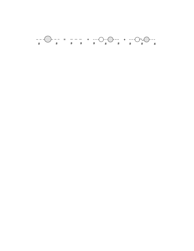
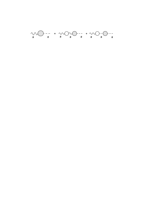
Figure 1: One-loop decomposition of exact propagators.

The corresponding equations are written as

$$G_{\mu\nu} \!\!\!=\!\!\! D_{\mu\nu}+D_{\mu\rho}\Pi^{\rho\sigma}G_{\sigma\nu}+D_{\mu\rho}\Pi^{\rho 5}G_{5\nu},$$ (3.2)

$$G_{55} \!\!\!=\!\!\! D_{55}+D_{55}\Pi^{55}G_{55}+D_{55}\Pi^{5\sigma}G_{\sigma 5},$$ (3.3)

$$G_{5\nu} \!\!\!=\!\!\! D_{55}\Pi^{5\sigma}G_{\sigma\nu}+D_{55}\Pi^{55}G_{5\nu},$$ (3.4)

$$G_{\mu 5} \!\!\!=\!\!\! D_{\mu\rho}\Pi^{\rho\sigma}G_{\sigma 5}+D_{\mu\rho}\Pi^{\rho 5}G_{55}.$$ (3.5)

The one-loop vacuum polarizations have the tensor structure given by

$$\Pi_{\mu\nu}=\Pi_{1}\eta_{\mu\nu}+\Pi_{2}p_{\mu}p_{\nu},\qquad\Pi_{\mu 5}=-\Pi_{\mu}^{~{}\,5}=\Pi_{3}p_{\mu}=\Pi_{5\mu},$$ (3.6)

where the explicit forms of $\Pi_{1}$, $\Pi_{2}$ and $\Pi_{3}$ will be given later. With these quantities, the one-loop exact propagators are solved as

$$G_{\mu\nu} \!\!\!=\!\!\! -{D_{55}\over 1+D_{55}\Pi_{1}}\eta_{\mu\nu}$$ (3.7)

$$+{D_{55}\left[(D_{55}\Pi_{2})(1-D_{55}\Pi^{55})+(D_{55}\Pi_{3})^{2}\right]p_{\mu}p_{\nu}\over(1+D_{55}\Pi_{1})\left[(1-D_{55}\Pi^{55})(1+D_{55}(\Pi_{1}+\Pi_{2}p^{2}))+(D_{55}\Pi_{3})^{2}p^{2}\right]},$$

$$G_{55} \!\!\!=\!\!\! {D_{55}(1+D_{55}(\Pi_{1}+\Pi_{2}p^{2}))\over(1-D_{55}\Pi^{55})(1+D_{55}(\Pi_{1}+\Pi_{2}p^{2}))+(D_{55}\Pi_{3})^{2}p^{2}},$$ (3.8)

$$G_{5\nu} \!\!\!=\!\!\! {D_{55}(D_{55}\Pi_{3})\over(1-D_{55}\Pi^{55})(1+D_{55}(\Pi_{1}+\Pi_{2}p^{2}))+(D_{55}\Pi_{3})^{2}p^{2}}p_{\nu},$$ (3.9)

where $G_{\nu 5}=G_{5\nu}$.

Now we perform the renormalization. From the Lagrangians (2.26), (2.27) and (2.28), the contributions of counterterms are led to

$$\Pi_{\mu\nu}^{ct}(p) \!\!\!=\!\!\! -i(p^{2}\eta_{\mu\nu}-p_{\mu}p_{\nu})\delta_{1}+{i\delta_{3}\over 1+\lambda}m_{As}^{2}\eta_{\mu\nu},$$ (3.10)

$$\Pi_{\mu 5}^{ct}(p) \!\!\!=\!\!\! {\delta_{4}\over 1+\lambda}m_{As}p_{\mu},\qquad\Pi_{55}^{ct}(p)={i\delta_{2}\over 1+\lambda}p^{2}.$$ (3.11)

Only three renormalization factors among $\delta_{1},\cdots,\delta_{4}$ are independent. All the divergence associated with $\Pi_{1},\Pi_{2},\Pi_{3},\Pi^{55}$ must be removed with three renormalization factors. As the first step, it is convenient to fix the renormalization condition for the off-diagonal component, $G_{5\nu}(m_{As}^{2})=0$. This condition yield

$$\Pi_{3}(m_{As}^{2})=0,$$ (3.12)

which corresponds to the fixing of $\delta_{4}$. For $\Pi_{3}=0$, the other propagators are simplified as

$$G_{\mu\nu} \!\!\!=\!\!\! -{D_{55}\over 1+D_{55}(\Pi_{1}+\Pi_{2}p^{2})}\left[\eta_{\mu\nu}+{D_{55}\Pi_{2}\over 1+D_{55}\Pi_{1}}(p^{2}\eta_{\mu\nu}-p_{\mu}p_{\nu})\right],$$ (3.13)

$$G_{55} \!\!\!=\!\!\! {D_{55}\over 1-D_{55}\Pi^{55}}.$$ (3.14)

For Eq. (3.13), $G_{\mu\nu}$, the term of $(p^{2}\eta_{\mu\nu}-p_{\mu}p_{\nu})$ is renormalized with the counterterm for $\delta_{1}$. The corresponding renormalization condition can be imposed as

$$\Pi_{2}(m_{As}^{2})=0.$$ (3.15)

As we will show explicitly, the divergent part for $\Pi_{1}$ and $\Pi^{55}$ satisfy $((\Pi_{1}+p^{2}\Pi_{2})/m_{As}^{2})_{\textrm{\scriptsize div}}=(\Pi^{55}/p^{2})_{\textrm{\scriptsize div}}$ at one-loop level. This reduces to $\delta_{2}=\delta_{3}$. Thus the renormalization can be chosen as

$$\Pi_{1}(m_{As}^{2})=0.$$ (3.16)

On the other hand, the finite part is $((\Pi_{1}+p^{2}\Pi_{2})/m_{As}^{2})\not=(\Pi^{55}/p^{2})$. This means that the propagator for $A_{y}$ receives finite mass corrections with $\Pi^{55}(m_{As}^{2})\not=0$. For the divergent part, it will be found in the following sections that at one-loop level, $\delta_{2}=\delta_{3}=\delta_{4}=(1+k)^{2}\delta_{1}$. Thus the momentum-dependent vacuum polarizations $\Pi_{1}(p^{2})$, $\Pi_{2}(p^{2})$, $\Pi_{3}(p^{2})$ and $\Pi^{55}(p^{2})$ can be achieved after the divergent part is fixed with the renormalization conditions (3.12), (3.15) and (3.16). From these equations, we can identify the asymptotic behavior of the $\Pi_{1}(p^{2})$, $\Pi_{2}(p^{2})$, $\Pi_{3}(p^{2})$ and $\Pi^{55}(p^{2})$. It needs to be checked if Lorentz invariance is preserved at high energy scales.

Renormalization for fermion self-energies would be given in a similar procedure. It may be technically complicated since one-loop self-energies are not diagonal with respect to Kaluza-Klein modes. This can be found from explicit one-loop amplitudes summarized in Appendix A. A feasible way to treat off-diagonal components has been developed in Ref. [16]. At the first step to address asymptotic behavior of the Lorentz violation, we are interest in not only Lorentz invariance but also gauge invariance. Both of these invariances can be simultaneously examined when the vacuum polarization rather than the self-energy is analyzed. Therefore we focus on the effects on the vacuum polarization for $A_{\mu}$ and $A_{y}$ and the issue for determining momentum-dependent amplitudes with external fermions will be left for future work.

4 Energy dependence of Lorentz violating terms and higher-dimensional Ward identity

Following the formalism of the previous section, we analyze explicit one-loop results for the Lorentz violation. The one-loop contributions for the vacuum polarization, $\Pi_{1}^{(1)}$, $\Pi_{2}^{(1)}$, $\Pi_{3}^{(1)}$ and $\Pi^{55(1)}$ are given via the dimensional regularization by

$$\Pi_{1}^{(1)}(p^{2}) \!\!\!=\!\!\! {8ig^{2}\over(4\pi)^{2}(1+k)}\int_{0}^{1}dx\left\{\left(z_{4}-\sum_{n_{p}=1}^{\infty}z_{3}e^{-{2z_{4}\over z_{3}}}\cdot\cos(2\pi n_{p}xs)\right)\right.$$ (4.1)

$$\times x(1-x)(p^{2}-m_{\psi s}^{2})$$

$$-\left.{1\over 4}\sum_{n_{p}=1}^{\infty}z_{3}(z_{3}+2z_{4})e^{-{2z_{4}\over z_{3}}}(1-2x)m_{\psi s}\sin(2\pi n_{p}xs)\right\},$$

$$\Pi_{2}^{(1)}(p^{2}) \!\!\!=\!\!\! -{8ig^{2}\over(4\pi)^{2}(1+k)}\int_{0}^{1}dx\left\{\left(z_{4}-\sum_{n_{p}=1}^{\infty}z_{3}e^{-{2z_{4}\over z_{3}}}\cdot\cos(2\pi n_{p}xs)\right)\right.$$ (4.2)

$$\left.\times x(1-x)\right\},$$

$$\Pi_{3}^{(1)}(p^{2}) \!\!\!=\!\!\! -{8ig^{2}{\cal N}\over(4\pi)^{2}(1+k)}\int_{0}^{1}dx\left\{\left(z_{4}-\sum_{n_{p}=1}^{\infty}z_{3}e^{-{2z_{4}\over z_{3}}}\cos(2\pi n_{p}xs)\right)\right.$$ (4.3)

$$\times x(1-x)m_{\psi s}$$

$$\left.+{1\over 4}\sum_{n_{p}=1}^{\infty}z_{3}(z_{3}+2z_{4})e^{-{2z_{4}\over z_{3}}}(1-2x)\sin(2\pi n_{p}xs)\right\},$$

$$\Pi^{55(1)}(p^{2}) \!\!\!=\!\!\! {8ig^{2}{\cal N}^{2}\over(4\pi)^{2}(1+k)}\int_{0}^{1}dx\left\{z_{4}x(1-x)p^{2}\right.$$ (4.4)

$$-{1\over 4}\sum_{n_{p}=1}^{\infty}\left[3z_{3}^{2}(z_{3}+2z_{4})+2z_{3}(2x(1-x)m_{\psi s}^{2})\right]e^{-{2z_{4}\over z_{3}}}\cos(2\pi n_{p}xs)$$

$$\left.+{1\over 4}\sum_{n_{p}=1}^{\infty}z_{3}(z_{3}+2z_{4})e^{-{2z_{4}\over z_{3}}}(1-2x)m_{\psi s}\sin(2\pi n_{p}xs)\right\},$$

where $z_{3}\equiv(1+k)/(n_{p}L)$ and $z_{4}\equiv\sqrt{x(1-x)(m_{\psi s}^{2}-p^{2})}$. In the above equations, the $n_{p}$-independent part is finite due to the dimensional regularization in spacetime with odd dimensions but it is potentially divergent. For the $n_{p}$-independent part, $(\Pi_{1}^{(1)}+p^{2}\Pi_{2}^{(1)})/m_{As}^{2}=\Pi^{55(1)}/p^{2}$ is satisfied.

From the renormalization conditions (3.12), (3.15) and (3.16), the renormalization factors $\delta_{1},\cdots,\delta_{4}$ are fixed. Then the renormalized vacuum polarizations are given by

$$\Pi_{j}(p^{2})=\Pi_{j}^{(1)}(p^{2})-\Pi_{j}^{(1)}(m_{As}^{2}),$$ (4.5)

$$\Pi^{55}(p^{2})=\Pi^{55(1)}(p^{2})$$

$$-ip^{2}\left[1-{i\Pi_{1}^{(1)}(m_{As}^{2})\over m_{As}^{2}}-{1\over 1+i\Pi_{2}^{(1)}(m_{As}^{2})}\left(1-\Pi_{3}^{(1)}(m_{As}^{2})-{i\Pi_{1}^{(1)}(m_{As}^{2})\over m_{As}^{2}}\right)^{2}\right],$$ (4.6)

where $j=1,2,3$. At high energies, the vacuum polarizations behave as

$$\Pi^{\mu\nu}(p^{2}) \!\!\!\to\!\!\! \Pi^{\mu\nu}_{\textrm{\scriptsize as}}(p^{2})=\left[-(p^{2}\eta^{\mu\nu}-p^{\mu}p^{\nu})-{\cal N}^{2}m_{As}^{2}\eta^{\mu\nu}\right]\Pi_{2}^{\textrm{\scriptsize as}}(p^{2}),$$ (4.7)

$$\Pi^{\mu 5}(p^{2}) \!\!\!\to\!\!\! \Pi^{\mu 5}_{\textrm{\scriptsize as}}(p^{2})=-i{\cal N}^{2}(p^{\mu}m_{As})\Pi_{2}^{\textrm{\scriptsize as}}(p^{2}),$$ (4.8)

$$\Pi^{55}(p^{2}) \!\!\!\to\!\!\! \Pi^{55}_{\textrm{\scriptsize as}}(p^{2})=-{\cal N}^{2}p^{2}\Pi_{2}^{\textrm{\scriptsize as}}(p^{2}),$$ (4.9)

where $\Pi_{2}^{\textrm{\scriptsize as}}(p^{2})\equiv-8ig^{2}(4\pi)^{-2}(1+k)^{-1}\int_{0}^{1}dx\,z_{4}x(1-x)$. In obtaining the asymptotic values (4.7), (4.8) and (4.9), we have employed the renormalization factors $Z_{A}$ and $Z_{5}$ and the renormalized coupling constant $\lambda$ so as to satisfy the renormalization conditions. Explicitly these constants are given by

$$Z_{A} \!\!\!=\!\!\! 1+i\Pi_{2}^{(1)}(m_{As}^{2}),$$ (4.10)

$$Z_{5} \!\!\!=\!\!\! {1\over 1+i\Pi_{2}^{(1)}(m_{As}^{2})}\left(1-\Pi_{3}^{(1)}(m_{As}^{2})-{i\Pi_{1}^{(1)}(m_{As}^{2})\over m_{As}^{2}}\right)^{2},$$ (4.11)

$$\lambda_{r} \!\!\!=\!\!\! \lambda-(1+\lambda){i\Pi_{1}^{(1)}(m_{As}^{2})\over m_{As}^{2}}.$$ (4.12)

where the subscript $r$ indicates a renormalized quantity again to avoid confusion. The equations (4.8) and (4.9) include ${\cal N}_{r}$ in which $\lambda_{r}$ obeys Eq. (4.12) and is generally nonvanishing. Thus the extra-dimensional Lorentz invariance is violated in a generic region in the parameter space at high energy scales. Especially $\lambda=0$ does not mean $\lambda_{r}=0$.

To identify the effect of the violation of translation invariance due to the brane, we consider the limit $L\to\infty$. For this limit, the factor $z_{3}$ approaches zero, $z_{3}\to 0$ as $L^{-1}$ so that the vacuum polarization become Eqs. (4.7), (4.8) and (4.9). Then $\lambda_{r}$ is given in Eq. (4.12). In the representation (4.12), the limit yields $\Pi_{1}^{(1)}(m_{As}^{2})\to 0$ as $L^{-3}$. Thus the couping constant for $L\to\infty$ is $\lambda_{r}\to\lambda$. Therefore the infinite compactification radius and zero original $\lambda$ can recover the higher-dimensional Lorentz invariance.

Now we move on to the issue of Ward identity. We compare the Lorentz violating case with a simple extension of the four-dimensional quantum electrodynamics. In a simple extension, the vacuum polarization has the form $\Pi_{5D}^{MN}=(p^{M}p^{N}-p^{L}p_{L}\eta^{MN})\Pi$. This is decomposed as

$$\Pi_{5D}^{\mu\nu}=\left[-\left(p^{2}\eta^{\mu\nu}-p^{\mu}p^{\nu}\right)+p_{5}^{2}\eta^{\mu\nu}\right]\Pi,\qquad\Pi_{5D}^{\mu 5}=(p^{\mu}p^{5})\Pi,\qquad\Pi_{5D}^{55}=p^{2}\,\Pi.$$ (4.13)

which satisfy the identities,

$$p_{\mu}\Pi_{5D}^{\mu\nu}+p_{5}\Pi_{5D}^{5\nu}=0,\qquad p_{\mu}\Pi_{5D}^{\mu 5}+p_{5}\Pi_{5D}^{55}=0.$$ (4.14)

On the other hand, the asymptotic vacuum polarization given in Eq. (4.7), (4.8) and (4.9) have the relation

$$p_{\mu}\Pi_{\textrm{\scriptsize as}}^{\mu\nu}+im_{As}\Pi_{\textrm{\scriptsize as}}^{5\nu}=0,\qquad p_{\mu}\Pi_{\textrm{\scriptsize as}}^{\mu 5}-im_{As}\Pi_{\textrm{\scriptsize as}}^{55}=0.$$ (4.15)

From the correspondence $\Pi_{\textrm{\scriptsize as}}^{\mu\nu}\leftrightarrow\Pi_{5D}^{\mu\nu}$, $\Pi_{\textrm{\scriptsize as}}^{\mu 5}\leftrightarrow i\Pi_{5D}^{\mu 5}$ and $\Pi_{\textrm{\scriptsize as}}^{55}\leftrightarrow\Pi_{5D}^{55}$, we find that the one-loop vacuum polarizations satisfy the five-dimensional Ward identity even without preserving the five-dimensional Lorentz invariance.

5 Furry’s theorem on orbifolds

So far we have examined the properties of the vacuum polarizations with an explicit diagrammatic calculation. In this section, we give a formal aspect in higher-dimensional gauge theory.

In the four-dimensional electrodynamics, the charge conjugation is a symmetry of the theory, $C|\Omega\rangle=|\Omega\rangle$, where $C$ denotes the charge conjugation and $|\Omega\rangle$ is the vacuum state. The electromagnetic current, $j^{\mu}=\bar{\psi}\gamma^{\mu}\psi$ changes sign under the charge conjugation, $Cj^{\mu}(x)C^{\dagger}=-j^{\mu}(x)$ so that its vacuum expectation value is vanishing, $\langle\Omega|Tj^{\mu}(x)|\Omega\rangle=0$. Furry’s theorem states that any vacuum vacuum expectation value of an odd number of electromagnetic currents is vanishing.

Now we consider a two-current function ${\cal M}^{\mu}_{Y}\equiv\langle Tj^{\mu}(x_{1})j_{Y}(x_{2})\rangle$ by introducing another operator $j_{Y}=\bar{\psi}\psi$ and by imaging gauge and Yukawa interactions for external lines. Here the ground state of the free theory with the symmetry of the charge conjugation is denoted as $\rangle$. Because of the charge conjugation $Cj_{Y}(x)C^{\dagger}=+j_{Y}(x)$, the two-current function ${\cal M}_{Y}^{\mu}$ is vanishing. At the first sight, the function ${\cal M}_{Y}^{\mu}$ with gauge and Yukawa interactions seems to look like the vacuum polarizations $\Pi^{\mu 5}$ and $\Pi_{5D}^{\mu 5}$. On the other hand, the vacuum polarization $\Pi_{5D}^{\mu 5}$ is not vanishing for nonzero $\Pi_{5D}^{\mu\nu}$ as seen from Eq. (4.13). We have also explicitly derived a nonzero $\Pi^{\mu 5}$. Thus the structure of $\Pi^{\mu 5}$ needs to be clarified from the viewpoint of Furry’s theorem.

The one-loop two-point function for $A_{\mu j}(x)$ and $A_{ys}(w)$ is given by

$${\cal N}{g^{2}\over 2L}\delta_{js}\int d^{4}x_{1}d^{4}x_{2}D_{j,\mu\rho}(x-x_{1})D_{s}(w-x_{2})\langle T{\cal O}_{Y}^{\rho}(x_{1},x_{2})\rangle,$$ (5.1)

with the two-current operator

$${\cal O}_{Y}^{\rho}(x_{1},x_{2}) \!\!\!\equiv\!\!\! j_{s,0}^{\rho}(x_{1})j_{0,s}(x_{2})-j_{0,s}^{\rho}(x_{1})j_{s,0}(x_{2})$$ (5.2)

$$-j_{n,\ell}^{\rho}(x_{1})j_{\ell,n}(x_{2})(\delta_{n+s,\ell}-\delta_{n,s+\ell})-j_{n,\ell}^{\rho 5}(x_{1})j_{\ell,n}^{5}(x_{2})\delta_{n+\ell,s}.$$

Here the currents with zero mode are given by $j_{I,J}^{\rho}=\bar{\psi}_{I}\gamma^{\rho}\psi_{J}$ and $j_{I,J}=\bar{\psi}_{I}\psi_{J}$, where $I,J=0,1,\cdots,\infty$ and the currents with $\gamma^{5}$ are given by $j_{n,\ell}^{\rho 5}=\bar{\psi}_{n}\gamma^{\rho}i\gamma^{5}\psi_{\ell}$ and $j_{\ell,n}^{5}=\bar{\psi}_{\ell}i\gamma^{5}\psi_{n}$. The charge conjugation yields a change of the overall factor and the interchange of indices,

$$Cj_{I,J}^{\rho}(x)C^{\dagger} \!\!\!=\!\!\! -j_{J,I}^{\rho}(x),\qquad Cj_{I,J}(x)C^{\dagger}=+j_{J,I}(x),$$ (5.3)

$$Cj_{n,\ell}^{\rho 5}(x)C^{\dagger} \!\!\!=\!\!\! +j_{\ell,n}^{\rho 5}(x),\qquad Cj_{n,\ell}^{5}(x)C^{\dagger}=+j_{\ell,n}^{\rho 5}(x).$$ (5.4)

From these equations, we obtain $C{\cal O}_{Y}^{\rho}(x_{1},x_{2})C^{\dagger}=+{\cal O}_{Y}^{\rho}(x_{1},x_{2})$. Therefore that $\Pi^{\mu 5}$ is not necessarily zero is consistent with Furry’s theorem. In Eq. (2.36), $\bar{\psi}_{n}P_{L}A_{yn}\psi_{0}$ and $\bar{\psi}_{0}P_{R}A_{yn}\psi_{n}$ have relative sign. If they have the same sign, the contribution from the first line in Eq. (5.2) would vanish. The role of the relative sign in the term $\bar{\psi}_{n}A_{ym}\psi_{\ell}$ in Eq. (2.36) is similar.

Application of Furry’s theorem in orbifold models may be given not only for two-point functions but also for other functions. For example, the vacuum expectation value of one current is vanishing, $\langle Tj_{n,n}^{\mu}(x)\rangle=0$, where the indices are the identical $n$. Because a nonzero $\Pi^{\mu 5}$ is expected from a nonzero $\Pi_{5D}^{MN}$, Furry’s theorem in effective four-dimensional theory may be related to the discrete symmetry in the original higher-dimensional theory. Due to the dependence of Lorentz transformation on the dimensionality of spacetime, it is nontrivial to introduce discrete symmetry such as $P$, $C$, $T$ in higher-dimensional theory [17, 18]. We leave further exploration of this issue for future work.

6 Conclusion

We have studied the momentum dependence of Lorentz violating terms in the field-theoretical context in electrodynamics on orbifolds. Here an explicit analysis has been performed for loop diagrams and renormalization. We have found that the extra-dimensional Lorentz invariance is violated in a generic region in the parameter space at high energy scales. In particular, even if the original action is higher-dimensional Lorentz invariant, it is violated by loop effects. While the higher-dimensional Lorentz invariance is lost, a higher-dimensional Ward identity has been found to be fulfilled for the one-loop vacuum polarization. Therefore higher-dimensional gauge invariance may be prior to higher-dimensional Lorentz invariance as a guiding principle in a high-energy field theory. We have also discussed Furry’s theorem in orbifold models to confirm the consistency about the vacuum polarizations.

The four-dimensional Lorentz violation has also been studied as a distinct topic of Lorentz violation. In the four-dimensional electrodynamics with Lorentz violation, it has been discussed that Pauli-Villars regularization is a useful choice associated with gauge invariance [19, 20, 21]. On the other hand, it has been shown that propagators corresponding to Pauli-Villars are radiatively generated in an orbifold model [22]. In this light, the Pauli-Villars regulator may be the necessity of an extra-dimensional model rather than a choice. These relations should be examined further.

Acknowledgments

This work is supported by Scientific Grants from the Ministry of Education and Science, Grant No. 20244028.

Appendix A Loop corrections

In this appendix, the details of loop corrections are given.

A.1 Diagrams and four-momentum integrals

We evaluate loop corrections by calculating the sum of diagrams for each Kaluza-Klein mode. Propagators are defined for four-dimensional fields. The tree-level propagators are diagonal with respect to Kaluza-Klein modes and are given by

$$D^{\mu\nu}(x-w) \!\!\!=\!\!\! \langle TA_{0}^{\mu}(x)A_{0}^{\nu}(w)\rangle=\int{d^{4}p\over(2\pi)^{4}}{-i\eta^{\mu\nu}\over p^{2}+i\epsilon}e^{-ip\cdot(x-w)}$$ (A.1)

$$D_{n}^{\mu\nu}(x-w) \!\!\!=\!\!\! \langle TA_{n}^{\mu}(x)A_{n}^{\nu}(w)\rangle=\int{d^{4}p\over(2\pi)^{4}}{-i\eta^{\mu\nu}\over p^{2}-m_{An}^{2}+i\epsilon}e^{-ip\cdot(x-w)}$$ (A.2)

$$D_{n}(x-w) \!\!\!=\!\!\! \langle TA_{yn}(x)A_{yn}(w)\rangle\int{d^{4}p\over(2\pi)^{4}}{i\over p^{2}-m_{An}^{2}+i\epsilon}e^{-ip\cdot(x-w)},$$ (A.3)

for bosons and

$$S(x-w) \!\!\!=\!\!\! \langle T\psi_{0}(x)\bar{\psi}_{0}(w)\rangle=\int{d^{4}p\over(2\pi)^{4}}P_{L}{ip\!\!\!/\over p^{2}+i\epsilon}e^{-ip\cdot(x-w)}$$ (A.4)

$$S_{n}(x-w) \!\!\!=\!\!\! \langle T\psi_{n}(x)\bar{\psi}_{n}(w)\rangle=\int{d^{4}p\over(2\pi)^{4}}{i(p\!\!\!/+m_{\psi n})\over p^{2}-m_{\psi n}^{2}+i\epsilon}e^{-ip\cdot(x-w)},$$ (A.5)

for fermions.

The vacuum polarizations for $A_{\mu}$ and $A_{y}$ involve the following momentum integrals:

$$I_{1}(\mu,\nu;m_{1},m_{2}) \!\!\!\equiv\!\!\! -{g^{2}\over 2L}\int{d^{4}p_{1}\over(2\pi)^{4}}\textrm{tr}\left({p\!\!\!/{}_{1}\over p_{1}^{2}-m_{1}^{2}}\gamma_{\mu}{p\!\!\!/{}_{1}+p\!\!\!/{}_{2}\over(p_{1}+p_{2})^{2}-m_{2}^{2}}\gamma_{\nu}\right),$$ (A.6)

$$I_{2}(\mu,\nu;m_{1},m_{2}) \!\!\!\equiv\!\!\! -{g^{2}\over 2L}\int{d^{4}p_{1}\over(2\pi)^{4}}\textrm{tr}\left({m_{1}\over p_{1}^{2}-m_{1}^{2}}\gamma_{\mu}{m_{2}\over(p_{1}+p_{2})^{2}-m_{2}^{2}}\gamma_{\nu}\right),$$ (A.7)

for two four-indices,

$$I_{1}(\mu;m_{1},m_{2}) \!\!\!\equiv\!\!\! -{g^{2}\over 2L}\int{d^{4}p_{1}\over(2\pi)^{4}}\textrm{tr}\left({m_{1}\over p_{1}^{2}-m_{1}^{2}}\gamma_{\mu}{p\!\!\!/{}_{1}+p\!\!\!/{}_{2}\over(p_{1}+p_{2})^{2}-m_{2}^{2}}\right),$$ (A.8)

$$I_{2}(\mu;m_{1},m_{2}) \!\!\!\equiv\!\!\! -{g^{2}\over 2L}\int{d^{4}p_{1}\over(2\pi)^{4}}\textrm{tr}\left({p\!\!\!/{}_{1}\over p_{1}^{2}-m_{1}^{2}}\gamma_{\mu}{m_{2}\over(p_{1}+p_{2})^{2}-m_{2}^{2}}\right),$$ (A.9)

for one four-index and

$$I_{1}(m_{1},m_{2}) \!\!\!\equiv\!\!\! {g^{2}\over 2L}\int{d^{4}p_{1}\over(2\pi)^{4}}\textrm{tr}\left({p\!\!\!/{}_{1}\over p_{1}^{2}-m_{1}^{2}}{p\!\!\!/{}_{1}+p\!\!\!/{}_{2}\over(p_{1}+p_{2})^{2}-m_{2}^{2}}\right),$$ (A.10)

$$I_{2}(m_{1},m_{2}) \!\!\!\equiv\!\!\! {g^{2}\over 2L}\int{d^{4}p_{1}\over(2\pi)^{4}}\textrm{tr}\left({m_{1}\over p_{1}^{2}-m_{1}^{2}}{m_{2}\over(p_{1}+p_{2})^{2}-m_{2}^{2}}\right),$$ (A.11)

for no four-indices. These satisfy a property $I_{1}(\mu;m_{2},m_{1})=-I_{2}(\mu;m_{1},m_{2})$.

The self-energies for $\psi$ involve the following momentum integrals:

$$B_{1}(m_{1},m_{2}) \!\!\!\equiv\!\!\! -{g^{2}\over 2L}\int{d^{4}p_{2}\over(2\pi)^{4}}\gamma^{\mu}{1\over p_{2}^{2}-m_{1}^{2}}{p\!\!\!/{}_{1}-p\!\!\!/{}_{2}\over(p_{1}-p_{2})^{2}-m_{2}^{2}}\gamma_{\mu},$$ (A.12)

$$B_{2}(m_{1},m_{2}) \!\!\!\equiv\!\!\! -{g^{2}\over 2L}\int{d^{4}p_{2}\over(2\pi)^{4}}\gamma^{\mu}{1\over p_{2}^{2}-m_{1}^{2}}{m_{2}\over(p_{1}-p_{2})^{2}-m_{2}^{2}}\gamma_{\mu},$$ (A.13)

$$E_{1}(m_{1},m_{2}) \!\!\!\equiv\!\!\! -{g^{2}\over 2L}\int{d^{4}p_{2}\over(2\pi)^{4}}{1\over p_{2}^{2}-m_{1}^{2}}{p\!\!\!/{}_{1}-p\!\!\!/{}_{2}\over(p_{1}-p_{2})^{2}-m_{2}^{2}},$$ (A.14)

$$E_{2}(m_{1},m_{2}) \!\!\!\equiv\!\!\! -{g^{2}\over 2L}\int{d^{4}p_{2}\over(2\pi)^{4}}{1\over p_{2}^{2}-m_{1}^{2}}{m_{2}\over(p_{1}-p_{2})^{2}-m_{2}^{2}}.$$ (A.15)

With these integral expressions, the vacuum polarizations are summarized as follows:

$$= \sum_{n=-\infty}^{\infty}\left\{I_{1}(\mu,\nu;m_{\psi n},m_{\psi n})+I_{2}(\mu,\nu;m_{\psi n},m_{\psi n})\right\},$$ (A.16)

(A.17)

(A.18)

(A.19)

The vacuum polarizations for $A_{\mu}$ and $A_{y}$ do not give rise to one-loop corrections for brane terms. The Kaluza-Klein modes for external lines are diagonal.

The fermion self-energies are summarized as follows:

$\displaystyle=$ $\displaystyle\sum_{n=-\infty}^{\infty}B_{1}(m_{An},m_{\psi n})P_{L}+B_{1}(0,0)P_{L},$ (A.20)

$\displaystyle=$ $\displaystyle\sqrt{2}\sum_{n=1}^{\infty}\left\{B_{1}(m_{An},m_{\psi n})P_{L}+B_{2}(m_{An},m_{\psi n})P_{R}\right\}\delta_{2n,s},$ (A.21)

(A.22)

(A.23)

$$+B_{1}(m_{Aj},0)i\gamma^{5}\delta_{js}$$

$$+\sum_{n=1}^{\infty}\left\{B_{1}(m_{An},m_{\psi,j+n})+B_{2}(m_{An},m_{\psi,j+n})\right\}\delta_{j+2n,s}$$

$$+\sum_{n=1}^{\infty}\left\{B_{1}(m_{An},m_{\psi,n+s})+B_{2}(m_{An},m_{\psi,n+s})\right\}\delta_{j,s+2n}$$

$$+\sum_{\ell=1}^{\infty}\left\{B_{1}(m_{A,\ell+s},m_{\psi\ell})+B_{2}(m_{A,\ell+s},m_{\psi\ell})\right\}i\gamma^{5}\delta_{j,s+2\ell}$$

$$+\sum_{\ell=1}^{\infty}\left\{B_{1}(m_{A,j+\ell},m_{\psi\ell})-B_{2}(m_{A,j+\ell},m_{\psi\ell})\right\}i\gamma^{5}\delta_{j+2\ell,s}$$

$$+\sum_{n=-\infty}^{\infty}\left\{B_{1}(m_{An},m_{\psi,j+n})+B_{2}(m_{An},m_{\psi,j+n})\right\}\delta_{js},$$

$\displaystyle=$ $\displaystyle{\cal N}^{2}\left[\sum_{n=-\infty}^{\infty}E_{1}(m_{An},m_{\psi n})P_{L}-E_{1}(0,0)P_{L}\right],$ (A.24)

$\displaystyle=$ $\displaystyle-\sqrt{2}{\cal N}^{2}\sum_{n=1}^{\infty}\left\{E_{1}(m_{An},m_{\psi n})P_{L}+E_{2}(m_{An},m_{\psi n})P_{R}\right\}\delta_{2n,s},$ (A.25)

(A.26)

(A.27)

$$-\sum_{n=1}^{\infty}\left\{E_{1}(m_{An},m_{\psi,n+s})+E_{2}(m_{An},m_{\psi,n+s})\right\}\delta_{j,s+2n}$$

$$-\sum_{n=1}^{\infty}\left\{E_{1}(m_{An},m_{\psi,j+n})+E_{2}(m_{An},m_{\psi,j+n})\right\}\delta_{j+2n,s}$$

$$+\sum_{\ell=1}^{\infty}i\gamma^{5}\left\{E_{1}(m_{A,j+\ell},m_{\psi\ell})+E_{2}(m_{A,j+\ell},m_{\psi\ell})\right\}\delta_{j+2\ell,s}$$

$$+\sum_{\ell=1}^{\infty}i\gamma^{5}\left\{E_{1}(m_{A,\ell+s},m_{\psi\ell})-E_{2}(m_{A,\ell+s},m_{\psi\ell})\right\}\delta_{j,s+2\ell}$$

$$+\sum_{n=-\infty}^{\infty}\left\{E_{1}(m_{An},m_{\psi,j+n})+E_{2}(m_{An},m_{\psi,j+n})\right\}\delta_{js}$$

$$-\left\{E_{1}(0,m_{\psi j})+E_{2}(0,m_{\psi j})\right\}\delta_{js}\bigg{]}.$$

For $(E_{1}+E_{2})$, the mode sum with $-\infty\leq n\leq\infty$ is regarded as a formal equation because $A_{yn}$ has no zero mode.

A.2 Evaluation of momentum integrals

We calculate the momentum integrals by introducing Feynman parameters and employing the dimensional regularization and the Poisson resummation.

The momentum integrals for $\Pi_{\mu\nu}$ are given by

$$\sum_{n=-\infty}^{\infty}\left(I_{1}(\mu,\nu;m_{\psi n},m_{\psi,n+s})+I_{2}(\mu,\nu;m_{\psi n},m_{\psi,n+s})\right)$$ (A.28)

$$\!\!\!=\!\!\! {8ig^{2}\over(4\pi)^{2}(1+k)}\int_{0}^{1}dx\left\{\left(z_{4}-\sum_{n_{p}=1}^{\infty}z_{3}e^{-{2z_{4}\over z_{3}}}\cdot\cos(2\pi n_{p}xs)\right)\right.$$

$$\times x(1-x)\left((p_{2}^{2}-m_{\psi s}^{2})\eta_{\mu\nu}-p_{2\mu}p_{2\nu}\right)$$

$$-\left.{1\over 4}\sum_{n_{p}=1}^{\infty}z_{3}(z_{3}+2z_{4})e^{-{2z_{4}\over z_{3}}}(1-2x)m_{\psi s}\sin(2\pi n_{p}xs)\eta_{\mu\nu}\right\}.$$

For $s=0$, the four-dimensional Ward identity is satisfied. It is also seen from the following equation,

$$I_{1}(\mu,\nu;m_{1},m_{2})+I_{2}(\mu,\nu;m_{1},m_{2})=-{8g^{2}\over L}\int_{0}^{1}dx\int{d^{d}\ell\over(2\pi)^{d}}\,{1\over\left[\ell^{2}-\Delta\right]^{2}}$$

$$\times\left[x(1-x)(p_{2}^{2}\eta_{\mu\nu}-p_{2\mu}p_{2\nu})+{1\over 2}(m_{1}-m_{2})(xm_{2}-(1-x)m_{1})\eta_{\mu\nu}\right],$$ (A.29)

where $\ell=p_{1}+xp_{2}$ and $\Delta=xm_{2}^{2}+(1-x)m_{2}^{2}-x(1-x)p_{2}^{2}$. In the main text, the letter of the external momentum is denoted as $p$ instead of $p_{2}$. The momentum integrals for $\Pi_{\mu 5}$ are given by

$$\sum_{n=-\infty}^{\infty}\left(I_{1}(\mu;m_{\psi n},m_{\psi,n+s})+I_{2}(\mu;m_{\psi n},m_{\psi,n+s})\right)$$ (A.30)

$$\!\!\!=\!\!\! -{8ig^{2}\over(4\pi)^{2}(1+k)}p_{2\mu}\int_{0}^{1}dx\left\{\left(z_{4}-\sum_{n_{p}=1}^{\infty}z_{3}e^{-{2z_{4}\over z_{3}}}\cos(2\pi n_{p}xs)\right)x(1-x)m_{\psi s}\right.$$

$$\left.+{1\over 4}\sum_{n_{p}=1}^{\infty}z_{3}(z_{3}+2z_{4})e^{-{2z_{4}\over z_{3}}}(1-2x)\sin(2\pi n_{p}xs)\right\}.$$

The momentum integrals for $\Pi_{55}$ are given by

$$\sum_{n=-\infty}^{\infty}\left(I_{1}(m_{\psi n},m_{\psi,n+s})+I_{2}(m_{\psi n},m_{\psi,n+s})\right)$$ (A.31)

$$\!\!\!=\!\!\! {8ig^{2}\over(4\pi)^{2}(1+k)}\int_{0}^{1}dx\left\{z_{4}x(1-x)p_{2}^{2}\right.$$

$$-{1\over 4}\sum_{n_{p}=1}^{\infty}\left[3z_{3}^{2}(z_{3}+2z_{4})+2z_{3}(2x(1-x)m_{\psi s}^{2})\right]e^{-{2z_{4}\over z_{3}}}\cos(2\pi n_{p}xs)$$

$$\left.+{1\over 4}\sum_{n_{p}=1}^{\infty}z_{3}(z_{3}+2z_{4})e^{-{2z_{4}\over z_{3}}}(1-2x)m_{\psi s}\sin(2\pi n_{p}xs)\right\}.$$

For fermion self-energies, the momentum integrals with $-\infty\leq n\leq\infty$ are given by

$$\sum_{n=-\infty}^{\infty}\left(B_{1}(m_{An},m_{\psi,n+s})+B_{2}(m_{An},m_{\psi,n+s})\right)=-{4ig^{2}\over(4\pi)^{2}}\int_{0}^{1}dx{1\over\sqrt{w}}$$

$$\times\left\{\left(w_{2}-\sum_{n_{p}=1}^{\infty}w_{1}e^{-{2w_{2}\over w_{1}}}\cos\left(2\pi n_{p}{(1+k)^{2}xs\over w}\right)\right)\right.(1-x)\left(p\!\!\!/{}_{1}-{2(1+\lambda)m_{\psi s}\over w}\right)$$

$$\left.+\sum_{n_{p}=1}^{\infty}{(1+k)\over\sqrt{w}}w_{1}(w_{1}+2w_{2})e^{-{2w_{2}\over w_{1}}}\sin\left(2\pi n_{p}{(1+k)^{2}xs\over w}\right)\right\}.$$ (A.32)

Here

$$w_{1} \!\!\!\equiv\!\!\! {\sqrt{w}\over n_{p}L},\qquad w_{2}\equiv\sqrt{x(1-x)\left({(1+\lambda)\over w}m_{\psi s}^{2}-p_{1}^{2}\right)},$$ (A.33)

$$w \!\!\!\equiv\!\!\! x(1+k)^{2}+(1-x)(1+\lambda).$$ (A.34)

The momentum integrals for $E_{1}$ and $E_{2}$ are obtained as with the relations

$$E_{1}(m_{1},m_{2})=-{1\over 2}B_{1}(m_{1},m_{2}),\qquad E_{2}(m_{1},m_{2})={1\over 4}B_{2}(m_{1},m_{2}).$$ (A.35)

References

• [1] J. Scherk and J. H. Schwarz, Phys. Lett.  B 82, 60 (1979).
• [2] J. Scherk and J. H. Schwarz, Nucl. Phys.  B 153, 61 (1979).
• [3] Y. Hosotani, Phys. Lett.  B 126, 309 (1983).
• [4] Y. Hosotani, Annals Phys.  190, 233 (1989).
• [5] E. A. Mirabelli and M. E. Peskin, Phys. Rev.  D 58, 065002 (1998) [arXiv:hep-th/9712214].
• [6] D. E. Kaplan, G. D. Kribs and M. Schmaltz, Phys. Rev.  D 62, 035010 (2000) [arXiv:hep-ph/9911293].
• [7] Z. Chacko, M. A. Luty, A. E. Nelson and E. Ponton, JHEP 0001, 003 (2000) [arXiv:hep-ph/9911323].
• [8] Y. Kawamura, Prog. Theor. Phys.  103, 613 (2000) [arXiv:hep-ph/9902423].
• [9] Y. Kawamura, Prog. Theor. Phys.  105, 999 (2001) [arXiv:hep-ph/0012125].
• [10] D. Diego, G. von Gersdorff and M. Quiros, JHEP 0511, 008 (2005) [arXiv:hep-ph/0505244].
• [11] N. Haba and N. Uekusa, arXiv:0911.2557 [hep-ph].
• [12] N. Uekusa, Mod. Phys. Lett.  A 23, 603 (2008) [arXiv:0704.2490 [hep-th]].
• [13] N. Uekusa, Int. J. Mod. Phys.  A 23, 3535 (2008) [arXiv:0803.1537 [hep-ph]].
• [14] N. Uekusa, Nucl. Phys.  B 812, 81 (2009) [arXiv:0806.3229 [hep-ph]].
• [15] T. G. Rizzo, JHEP 0509, 036 (2005) [arXiv:hep-ph/0506056].
• [16] N. Uekusa, arXiv:1002.1904 [hep-ph].
• [17] Y. Adachi, C. S. Lim and N. Maru, Phys. Rev.  D 80, 055025 (2009) [arXiv:0905.1022 [hep-ph]].
• [18] C. S. Lim, N. Maru and K. Nishiwaki, arXiv:0910.2314 [hep-ph].
• [19] R. Jackiw and V. A. Kostelecky, Phys. Rev. Lett.  82, 3572 (1999) [arXiv:hep-ph/9901358].
• [20] M. Perez-Victoria, JHEP 0104, 032 (2001) [arXiv:hep-th/0102021].
• [21] B. Altschul, Phys. Rev.  D 70, 101701 (2004) [arXiv:hep-th/0407172].
• [22] N. Uekusa, Nucl. Phys.  B 827, 311 (2010) [arXiv:0909.0825 [hep-ph]].