Non-Markovian entanglement dynamics in coupled superconducting qubit systems

Abstract

We theoretically analyze the entanglement generation and dynamics by coupled Josephson junction qubits. Considering a current-biased Josephson junction (CBJJ), we generate maximally entangled states. In particular, the entanglement dynamics is considered as a function of the decoherence parameters, such as the temperature, the ratio $r\equiv\omega_{c}/\omega_{0}$ between the reservoir cutoff frequency $\omega_{c}$ and the system oscillator frequency $\omega_{0}$, and the energy levels split of the superconducting circuits in the non-Markovian master equation. We analyzed the entanglement sudden death (ESD) and entanglement sudden birth (ESB) by the non-Markovian master equation. Furthermore, we find that the larger the ratio $r$ and the thermal energy $k_{B}T$, the shorter the decoherence. In this superconducting qubit system we find that the entanglement can be controlled and the ESD time can be prolonged by adjusting the temperature and the superconducting phases $\Phi_{k}$ which split the energy levels.

1 Introduction

Entanglement is one of the remarkable features of quantum mechanics. Briefly, entanglement refers to correlated behavior of two or more particles that cannot be described classically, the properties of one particle can depend on those of another (typically distant) particle in a way that only quantum mechanics can explain. Einstein-Podolsky-Rosen (EPR) entangled states, probably the simplest and most interesting entangled states, have been employed not only to test Bell’s inequality, but also to realize quantum cryptography, quantum teleportation, and quantum computation Stolze:08 ; Bellac:06 ; Mermin:07 ; Rowe:01 ; Nori:09 . It has become clear that entanglement is a new resource for tasks that cannot be performed by means of classical resources Bennett ; Zoller . Although many results have been obtained (for example, see the review papers Amico ; Horodecki ), the theory of quantum entanglement has open questions, like (i) how to optimally detect entanglement theoretically and practically; (ii) how to reverse the inevitable process of degradation of entanglement; and (iii) how to characterize, quantify and control entanglement. The focus of this paper is a theory study of entanglement dynamics and control in a coupled Josephson junction system.

Superconducting quantum circuits You2 are the subject of intense research at present. Josephson devices can serve as quantum bits (qubits) in quantum information and that quantum logic operations could be performed by controlling gate voltages or magnetic fields You2 . Moreover, for its scalable and macroscopic property, Josephson junctions offer one of the most promising candidate served as hardware implementation of quantum computers Berkley ; McDermott ; Liu ; Dimitris ; Wei ; Schulz ; You . The charge, flux, and phase qubits are three basic types of superconducting qubits You2 depending on which dynamical variable is most well defined. Operations with multiple superconducting qubits have also been performed. Several types of Josephson-junction qubits have been proposed and explored in the laboratory. The first solid-state quantum gate has been demonstrated with charge qubits Yamamoto . For flux qubits, two-qubit coupling and a controllable coupling mechanism have been realized Hime ; Niskanen . However, due to the difficulty to decouple the qubits from the environments in solid-state systems, only the two-qubit entanglement of the superconducting qubits has been observed in experiments Steffen , while the entangled states up to eight Haffner or six photonic Pan qubits have been experimentally reported. Therefore, the future generation of multi-particle entangled states for solid state quantum computation would be a significant, step towards quantum information processing. A challenge is quantum decoherence, because any pure quantum state used evolves into a mixed state due to the unavoidable interactions with the environment. Decoherence describes the environment-induced suppression of the quantum mechanical coherence properties and interference ability, which transforms the quantum system into classical one. The description of this process requires us to take into account not only the degrees of freedom of the system of interest, but also those of the environment. Decoherence of the Josephson junction qubits is considered to be the major impediment for quantum logic gate operations. Thus, short coherence times limit both the manipulation of the qubit state and information storage. In all superconducting qubits, both the spectrum of charge noise and the critical current fluctuations as it is display a $1/f$ behavior at low frequencies. Moreover, both charge noise and critical current fluctuations can be phenomenologically explained by modeling the environment as a collection of discrete bistable fluctuators, representing charged impurities hopping between different locations in the substrate or in the tunnel barrier. Many efforts Robert searched for decoherence mechanisms that suppress the decoherence time.

On the path to quantum computing, superconducting qubits You2 are clearly among the most promising candidates. References Ashhab1 ; Ashhab2 ; Ashhab3 showed that such two-level systems can themselves be used as qubits, allowing for a well controlled initialization, universal sets of quantum gates, and readout. Thus, a single current-biased Josephson junction can be considered as a multi-qubit register. It can be coupled to other junctions to allow the application of quantum gates to an arbitrary pair of qubits in the system. These results Ashhab1 ; Ashhab2 ; Ashhab3 indicate an alternative way to control qubits coupled to naturally formed quantum two-level systems, for improved superconducting quantum information processing. Nevertheless, the path is long, and there are quantitative technological obstacles to be overcome, notably increasing the decoherence time, improving the fidelity of the read-out, and strengthening the entanglement distillation in its dynamics.

Within the theory of open quantum system Onofrio:93 ; Onofrio:96 ; Breuer the dissipative dynamics can be described by the master equation of the reduced density matrix. In general this equation is obtained by tracing over the environment variables, after performing a series of approximations. The Born-Markovian approximation is usually used in deducing the master equation, which neglects the correlations between the system and the reservoir. The Markovian approximation leads to a master equation which can be cast into the so called Lindblad form. Master equations in the Lindblad form are characterized by the fact that the dynamical group of the system satisfies both the semigroup property and the complete positivity condition. However, in the superconducting qubit system the Markovian approximation is not justified Chirolli ; JSZhang . In recent years, non-Markovian quantum dissipative systems Cui1 ; YJZhang ; Lajos ; Suominen ; Gambetta ; Vacchini ; Wolf ; Burkard ; Breuer:09 ; Piilo:09 have attracted much attention due to its fundamental importance in quantum information processing .

In this paper, we will focus on the dynamics of the generated superconducting entangled state in a non-Markovian environment by using the master equation method. It determines how much quantum information can be reliably transmitted over the noisy quantum channels. We then discuss schemes for controlling the entanglement between the superconducting quantum circuits. Nowadays, quantum-state engineering, i.e., active control over the coherent dynamics of suitable quantum-mechanical systems, has become a fascinating prospect of modern physics Ashhab1 ; Ashhab2 ; Ashhab3 . Quantum decoherence and entanglement control pave the way for future long coherent time quantum information processing and computation.

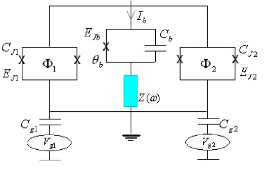
Figure 1: Color online) Schematic diagram of the coupled-qubit circuit with a biased-current source of impedance $Z(\omega)$. Two Josephson charge qubits are controllably coupled to a common current-biased Josephson junction, which operates as a Josephson phase qubit and acts as a coupler. Two Josephson qubits and current-biased Josephson junction with the electromagnetic environment represented by the impedance $Z(\omega)$.

This paper is organized as follows. We first introduce superconducting qubits decoherence and the quantum non-Markovian master equation for driven open quantum systems. In Sec. II, we shall briefly recall the physics of the Cooper pair box, and give the model of the superconducting qubits interacting with the bath. In Sec. III, we consider the entanglement dynamics by the non-Markovian master equation. Both entanglement sudden death (ESD) and entanglement sudden birth (ESB) are analyzed by numerical simulation. Conclusions are given in Sec. IV.

2 The model

In this work, we present an experimentally implementable method to couple two Josephson charge qubits and to generate, detect and control of macroscopic quantum entangled states in this charge-qubit system. Let us study the superconducting circuit shown in Fig.1, where two single Cooper pair boxes (CPBs) are connected via a common bus, i.e., a current-biased Josephson junction (CBJJ). Each qubit consists of a gate electrode of capacitance $C_{g}$ and a single Cooper pair box with two ultrasmall identical Josephson junctions of capacitance $C_{J}$ and Josephson energy $E_{J}$, forming a superconducting quantum interference device (SQUID) ring threaded by a flux $\Phi$ and with a gate voltage $V$. The superconducting phase difference across the $k$th qubit is represented by $\Phi_{k},~{}~{}k=1,2$. The large CBJJ has capacitance $C_{b}$, phase drop $\theta_{b}$, Josephson energy $E_{b}$, and a bias current $I_{b}$. The reason for this choice is that this circuit can be easily generalized to include more qubits, coupled by a common CBJJ. For the detail of controllable coupling of superconducting qubits, one can refer to You:031 ; You:032 ; You:05 ; Wei:05 ; Wei:06 ; Wei:062 ; Ashhab:06 ; Ashhab:07 ; Liu:07 .The Hamiltonian without dissipation can be written as

$$\hat{H}_{s}=\sum_{k=1}^{2}4E_{c}(\hat{n}_{k}-n_{gk})^{2}-E_{J}(\Phi_{k})\cos\hat{\theta}_{k}+\hat{H}_{kb}+\hat{H}_{b},$$ (1)

where

$$\hat{H}_{kb} = \pi C_{g}E_{J}(\Phi_{k})\hat{\theta}_{b}\sin\hat{\theta}_{k}/\left[\Phi_{0}(C_{g}+2C_{J}^{0})\right],$$

$$\hat{H}_{b} = \hat{Q}_{b}^{2}/(2\tilde{C}_{b})-E_{Jb}\cos\hat{\theta}_{b}-\Phi_{0}I_{b}/(2\pi\hat{\theta}_{b}).$$

Here $E_{c}=e^{2}/[2(C_{g}+2C_{J}^{0})]$ is the single-electron charging energy of a single CPB. For simplicity, we assume that $E_{c}$ and $E_{J}^{0}$ are the same for the two CPBs. $C_{g}$ and $C_{g}^{0}$ are the capacitances of the gate electrode and identical Josephson junctions, respectively. The Josephson energy $E_{J}(\Phi_{k})$ of the $k$th dc SQUID is $E_{J}(\Phi_{k})=2E_{J}^{0}\cos(\pi\Phi_{k}/\Phi_{0})$, where $E_{J}^{0}$ represents the Josephson energy of a single Josephson junction, $\Phi_{k}$ denotes the external flux piercing the SQUID loop of the $j$-th CPB, and $\Phi_{0}$ is the flux quantum. $\hat{Q}_{b}=2\pi\hat{p}_{b}/\Phi_{0}$ is the operator of charges on the CBJJ. $E_{Jb}$ and $\tilde{C}_{b}=C_{Jb}+\sum_{k=1}^{2}(C_{Jk}^{-1}+C_{gk}^{-1})^{-1}=C_{Jb}+2((2C_{J}^{0})^{-1}+C_{g}^{-1})^{-1}$ are the Josephson energy and effective capacitance of the CBJJ, respectively. Also, $\Phi_{0}=h/(2e)$ is the flux quantum. The operators $\hat{n}_{k}$ and $\hat{\theta}_{k}$ satisfy the commutation relations $[\hat{\theta}_{k},\hat{n}_{k}]=i$ (we assume $\hbar=1$), which describe the excess number of Cooper pairs and the effective phase across the junctions in the $k$-th CPB, respectively. In addition, the phase operator $\hat{\theta}_{b}$ for the CBJJ and its conjugate $\hat{p}_{b}$ satisfy another commutation relation $[\hat{\theta}_{b},\hat{p}_{b}]=i$.

Suppose that the CPBs are biased at the charge degenerate point, such that $n_{gk}=C_{gk}V_{k}/(2e)=1/2$ (when $V_{k}=e/C_{gk}$). The two energy levels of the $k$-th CPB corresponding to $n_{k}=0,1$ are close to each other and far separated from other high-energy levels. In this case, they behave as effective two level systems (with the basis $\left\{|\uparrow_{k}\rangle=|n_{k}=0\rangle,~{}~{}|\downarrow_{k}\rangle=|n_{k}=1\rangle\right\}$) Wei1 . It is well known that the CBJJ can be approximated as a harmonic oscillator Wei1 ; Wei ; Zhang1 ; Zhang2 , if it is biased as $I_{b}\ll I_{0}=2\pi E_{Jb}/{\Phi_{0}}$. Here, we consider a very different case, i.e., the biased dc current $I_{b}$ is slightly smaller than the critical current $I_{0}$, and thus the CBJJ has only a few bound states. The two lowest energy states $|0_{b}\rangle$ and $|1_{b}\rangle$ are selected to define a Josephson phase qubit acting as a two-level date bus. Under such condition, the Hamiltonian of the CBJJ reduces to $\hat{H}_{b}=\hbar\omega_{b}\hat{\sigma}_{b}^{z}$, with $\hat{\sigma}_{b}^{z}=|0_{b}\rangle\langle 0_{b}|-|1_{b}\rangle\langle 1_{b}|$ being the standard Pauli operator and $\omega_{b}=E_{b1}-E_{b0}$ the eigenfrequency.

Under the rotating-wave approximation, the Hamiltonian $H$ can be rewritten as

$$H_{s} = \sum_{k=1}^{2}\left(\frac{E_{Jk}(\Phi_{k})}{2}\sigma_{z}^{(k)}-\frac{E_{Ck}(n_{gk})}{2}\sigma_{x}^{(k)}\right)+\omega_{b}\sigma_{z}^{(b)}$$ (2)

$$+J\left(\sigma_{+}^{1}\sigma_{-}^{2}+\sigma_{+}^{2}\sigma_{-}^{1}\right),$$

with

$$\begin{array}[]{rcl}\sigma_{x}^{(k)}&=&|+\rangle_{kk}\langle-|+|-\rangle_{kk}\langle+|,\\ \sigma_{y}^{(k)}&=&-i|+\rangle_{kk}\langle-|+i|-\rangle_{kk}\langle+|,\\ \sigma_{z}^{(k)}&=&|+\rangle_{kk}\langle+|-|-\rangle_{kk}\langle-|,\end{array}$$

and $\sigma_{\pm}^{(k)}=\left(\sigma_{x}^{(k)}\pm i\sigma_{y}^{(k)}\right)/2$, where $|+\rangle_{k}=(|0\rangle_{k}+|1\rangle_{k})/\sqrt{2}$ and $|-\rangle_{k}=(|0\rangle_{k}-|1\rangle)/\sqrt{2}$. Note that, the charging energy $E_{Ck}(n_{gk})=2e^{2}(1-2n_{gk})/C_{k}$ of the $k$-th Josephson charge qubit can be switched off by setting the gate voltage $V_{k}$ such that $n_{gk}=1/2$. Also, by adjusting the external flux $\Phi_{k}$, the Josephson energy of the $k$-th qubit $E_{Jk}(\Phi_{k})=2E^{0}_{J}\cos(\pi\Phi_{k}/\Phi_{0})$ can be set to the strongest coupling $(\Phi_{k}=0)$ and the decoupling $(\Phi_{k}=\Phi_{0}/2)$. This achieves the controllability of the present quantum circuit. The coefficient $J$ is the coupling strength between the $k$-th qubit and Josephson junction with $J=\lambda_{1}\lambda_{2}/E_{c},~{}~{}\lambda_{k}=2E_{J}^{0}\sin(\Phi_{k}/2)$.

Obviously, if we assume the two qubits are both at the charge degenerate point $n_{gk}=1/2$, and $\Phi_{k}=\Phi_{0}/2$ with the separated initial state $|g\rangle_{b}|g\rangle_{1}|e\rangle_{2}$, the evolution operator of the corresponding two qubit system is given by

$$U(t)=\exp\left[-iJt(\sigma_{+}^{1}\sigma_{-}^{2}+\sigma_{+}^{2}\sigma_{-}^{1})-i\omega_{b}t\sigma_{z}^{(b)}\right],$$ (3)

and the system’s evolution is given by

$$U(t)|g\rangle_{b}|g\rangle_{1}|e\rangle_{2}=e^{-i\omega_{b}t\sigma_{z}^{(b)}}|g\rangle_{b}e^{-iJt(\sigma_{+}^{1}\sigma_{-}^{2}+\sigma_{+}^{2}\sigma_{-}^{1})}|g\rangle_{1}|e\rangle_{2}$$

$$=(\cos\omega_{b}t+i\sin\omega_{b}t)|g\rangle_{b}\left[\cos Jt|g\rangle_{1}|e\rangle_{2}-i\sin Jt|e\rangle_{1}|g\rangle_{2}\right].$$

If we choose $Jt=\pi/4$, we can obtain the maximally entangled state $|\Psi\rangle=(|g\rangle_{1}|e\rangle_{2}-i|e\rangle_{1}|g\rangle_{2})/\sqrt{2}$.

3 Entanglement dynamics

3.1 Markovian and non-Markovian master equations

We account for the dissipation due to electromagnetic fluctuations. They can be modeled by an effective impedance $Z(\omega)$, placed in series with the voltage source and producing a fluctuating voltage. The impedance is embedded in the circuit shown in Fig.1, which further modifies the spectrum of voltage fluctuations. In general, the environment consists of a large set of harmonic oscillators, each of which interacts weakly with the system of interest, i.e. $H_{bath}=\sum_{i}\left[\frac{p_{i}^{2}}{2m_{i}}+\frac{m_{i}w_{i}^{2}}{2}x_{i}^{2}\right]$. As mentioned in Sec. 1, we will use the master equation method to study the entanglement dynamics and control.

The analysis of the time evolution of open quantum system plays an important role in many applications of modern physics. With the Born-Markovian approximation the dynamics is governed by a master equation of relatively simple form Breuer

$$\frac{d}{dt}\rho(t)=-i[\hat{H}_{s}(t),\rho(t)]+\sum_{m}\gamma_{m}\mathcal{D}[C_{m}]\rho(t),$$ (5)

with a time-independent generator in the Lindblad form. This is the most general form for the generator of a quantum dynamical semigroup. The Hamiltonian $\hat{H}_{S}(t)$ describes the coherent part of the time evolution. Non-negative quantities $\gamma_{m}$ play the role of relaxation rates for the different decay modes of the open system. The operators $C_{m}$ are usually referred to as Lindblad operators which represent the various decay modes, and the corresponding density matrix equation (5) is called the Lindblad master equation. The solution of Eq. (5) can be written in terms of a linear map $V(t)=\exp(\mathcal{L}t)$ that transforms the initial state $\rho(0)$ into the state $\rho(t)=V(t)\rho(0)$ at time $t$. The physical interpretation of this map $V(t)$ requires that it preserves the trace and the positivity of the density matrix $\rho(t)$. The most important physical assumption which underlies Eq. (5) is the validity of the Markovian approximation of short environmental correlation times. With this approximation, the environment acts as a sink for the system information. Due to the system-reservoir interaction, the system of interest loses information on its state into the environment, and this lost information does not play any further role in the system dynamics.

If the environment has a non-trivial structure, then the seemingly lost information can return to the system at a later time leading to non-Markovian dynamics with memory. This memory effect is the essence of non-Markovian dynamics Cui1 ; Lajos ; Suominen ; Gambetta ; Vacchini ; Wolf ; Burkard ; Breuer:09 ; Piilo:09 , which is characterized by pronounced memory effects, finite revival times and non-exponential relaxation and decoherence. Non-Markovian dynamics plays an important role in many fields of physics, such as quantum optics, quantum information, quantum chemistry process, especially in solid state physics Breuer:09 . As a consequence the theoretical treatment of non-Markovian quantum dynamics is extremely demanding. However, in order to take into account quantum memory effects, an integro-differential equation is needed which has complex mathematical structure, thus preventing generally to solve the dynamics of the system of interest. An appropriate scheme is the time-covolutionless (TCL) projection operator technique Breuer ; Breuer:09 ; Piilo:09 which leads to a time-local first order differential equation for the density matrix.

By tracing out the bath degrees of freedom, we find for $\rho$ a non-Markovian evolution equation

$$\frac{d}{dt}\rho(t)=-i[\hat{H}_{s}(t),\rho(t)]+\sum_{m}\Delta_{m}(t)\mathcal{D}[C_{m}(t)]\rho(t).$$ (6)

with the super-operator $\mathcal{D}[L]\rho=L\rho L^{{\dagger}}-\frac{1}{2}L^{{\dagger}}L\rho-\frac{1}{2}\rho L^{{\dagger}}L$. The first term describes the unitary part of the evolution. The latter involves a summation over the various decay channels labeled by $m$ with corresponding time-dependent decay rates $\Delta_{m}(t)$ and arbitrary time-dependent system operators $C_{m}(t)$. In the simplest case, the rates $\Delta_{m}$ as well as the Hamiltonian $\hat{H}_{s}$ and the operators $C_{m}$ are assumed to be time-independent, that is, it is the Markovian case. Note that, for arbitrary time-dependent operators $\hat{H}_{s}(t)$ and $C_{m}(t)$, and for $\Delta_{m}(t)\geq 0$ the generator of the master equation (6) is still in Lindblad form at each fixed time $t$, which may be considered as time-dependent quantum Markovian process. However, if one or several of the $\Delta_{m}(t)$ become temporarily negative, which expresses the presence of strong memory effects in the reduced system dynamics, the process is then said to be non-Markovian.

For the system considered in Fig.1, two Josephson junction qubits coupled by the common current-biased Josephson junction, the bipartite dynamics is

$$\frac{d\rho(t)}{dt}=-i[H_{s},\rho]+\sum_{k=1}^{2}(\Gamma_{1}D[\sigma_{k}^{-}]\rho+\Gamma_{2}D[\sigma_{k}^{+}]\rho),$$ (7)

where $\Gamma_{1}=\Delta(t)+\gamma(t)$ and $\Gamma_{2}=\Delta(t)-\gamma(t)$. The time dependent coefficients $\Delta(t)$ and $\gamma(t)$ are diffusive term and damping term, which can be written as follows

$$\Delta(t)=\int_{0}^{t}d\tau k(\tau)\cos(\omega\tau),$$

$$\gamma(t)=\int_{0}^{t}d\tau\mu(\tau)\sin(\omega\tau),$$ (8)

with

$$k(\tau)=2\int_{0}^{\infty}d\omega J(\omega)\coth[\hbar\omega/2k_{B}T]\cos(\omega\tau),$$

$$\mu(\tau)=2\int_{0}^{\infty}d\omega J(\omega)\sin(\omega\tau),$$ (9)

being the noise and the dissipation kernels, respectively. In this paper we choose the Ohmic spectral density with a Lorentz-Drude cutoff function,

$$J(\omega)=\frac{2\gamma_{0}}{\pi}\omega\frac{\omega_{c}^{2}}{\omega_{c}^{2}+\omega^{2}},$$ (10)

where $\gamma_{0}$ is the frequency-independent damping constant and usually assumed to be $1$. $\omega$ is the frequency of the bath, and $\omega_{c}$ is the high-frequency cutoff. The analytic expression for the coefficients $\gamma(t)$and $\Delta(t)$ are given in Cui1 .

3.2 Measuring entanglement

Entanglement measure quantifies how much entanglement is contained in a quantum state. The entanglement measure for a state is zero iff the state is separable, and the bigger is the entanglement measure, then more entangled is the state. By axiomatic approach, (i) it is any nonnegative real function of a state which can not increase under local operations and classical communication (LOCC) (so called monotonicity) Brandao ; (ii) it is zero for separable states; (iii) and/or it satisfies normalization, asymptotic continuity, and convexity. There are operational entanglement measures such as distillable entanglement, distillable key and entanglement cost, as well as abstractly defined measures such as ones based on convex roof construction (e.g., concurrence and entanglement of formation) or based on a distance from a set of separable states such as the relative entropy of entanglement Horodecki . One of the most famous measures of entanglement is the Wootters’ concurrence Wootters of two-qubit system. We will use it to study the entanglement dynamics and obtain the entanglement transfers Maruyama:07 ; Cui2 ; Cui3 . For a system described by a density matrix $\rho$, the concurrence $\mathcal{C}(\rho)$ is

$$\mathcal{C}(\rho)=\max(0,\sqrt{\lambda_{1}}-\sqrt{\lambda_{2}}-\sqrt{\lambda_{3}}-\sqrt{\lambda_{4}}),$$ (11)

where $\lambda_{1},\lambda_{2},\lambda_{3}$, and $\lambda_{4}$ are the eigenvalues (with $\lambda_{1}$ the largest one) of the “spin-flipped” density operator $\zeta=\rho(\sigma_{y}^{A}\otimes\sigma_{y}^{B})\rho^{*}(\sigma_{y}^{A}\otimes\sigma_{y}^{B})$, where $\rho^{*}$ denotes the complex conjugate of $\rho$ and $\sigma_{y}$ is the Pauli matrix. $\mathcal{C}$ ranges in magnitude from 0 for a disentanglement state to 1 for a maximally entanglement state.

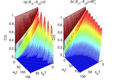
Figure 2: Color online) Non-Markovian entanglement concurrence $C_{\rho}(t)$ dynamics as a function of the thermal energy “$k_{B}T$” for the conditions $|E_{J1}-E_{J2}|=0$ and $|E_{J1}-E_{J2}|=4E_{J}^{0}$, respectively.

The initial state chosen is the previous generated maximal entangled state, $|\Psi\rangle=(|g\rangle_{1}|e\rangle_{2}-i|e\rangle_{1}|g\rangle_{2})/\sqrt{2}$, which is an “X” form mixed state Yu1 ; Yu2 ; Yu3 that has non-zero elements only along the main diagonal and anti-diagonal. The general form of an “X” density matrix is as follows

$$\rho=\left(\begin{array}[]{cccc}a&0&0&m+in\\ 0&b&e+if&0\\ 0&e-if&c&0\\ m-in&0&0&d\end{array}\right).$$ (12)

Such states are general enough to include states such as the Werner states, the maximally entangled mixed states (MEMSs) and the Bell states; and it also arises in a wide variety of physical situations. A remarkable aspect of the “X” form mixed states is that the time evolution of the master equation (5) determined by the initial “X” form is maintained during the evolution. This particular form of the density matrix allows us to analytically express the concurrence at time $t$ as

$$\mathcal{C}_{\rho}^{X}(t)=2\max\{0,K_{1}(t),K_{2}(t)\},$$ (13)

where $K_{1}(t)=\sqrt{e^{2}(t)+f^{2}(t)}-\sqrt{a(t)d(t)}$, and $K_{2}(t)=\sqrt{m^{2}(t)+n^{2}(t)}-\sqrt{b(t)c(t)}$.

The non-Markovian master equation (7) is equivalent to a system of coupled differential equations, the first four of which describe the time evolution of the populations, namely

$$\dot{a} = -2(\Delta(t)+\gamma(t))a+(\Delta(t)-\gamma(t))(b+c)$$

$$\dot{b} = (\Delta(t)+\gamma(t))a-2\Delta(t)b+(\Delta(t)-\gamma(t))d-2Jf$$

$$\dot{c} = (\Delta(t)+\gamma(t))a-2\Delta(t)c+(\Delta(t)-\gamma(t))d+2Jf$$

$$\dot{d} = (\Delta(t)+\gamma(t))(b+c)-2(\Delta(t)-\gamma(t))d,$$ (14)

while the other equations describe the time evolution of the coherence:

$$\dot{e} = -2\Delta(t)e+(E_{J1}-E_{J2})f$$

$$\dot{f} = -2\Delta(t)f-(E_{J1}-E_{J2})e+J(b-c)$$

$$\dot{m} = -2\Delta(t)m+(E_{J1}+E_{J2})n$$

$$\dot{n} = -2\Delta(t)n-(E_{J1}+E_{J2})m.$$ (15)

In the following subsection we will bring to light the features characterizing the dynamics of superconducting entanglement.

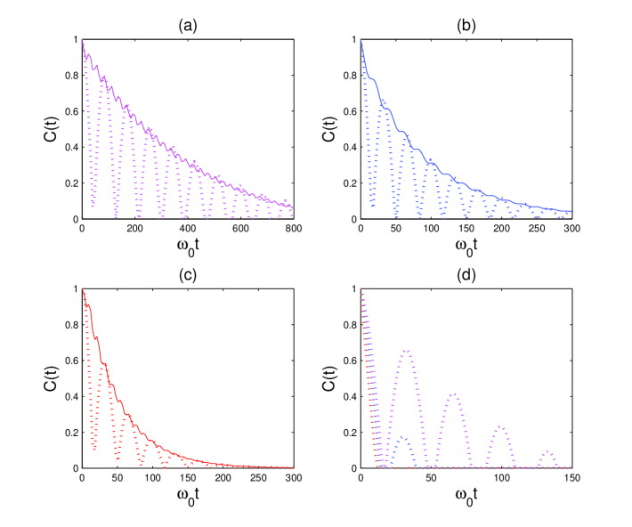
Figure 3: (Color online) The evolutions of the concurrence $\mathcal{C}(t)$ of the superconducting qubits in a low temperature environment with $k_{B}T=0.03\omega_{0}$ for (a) ratio $r\equiv\omega_{c}/\omega_{0}=0.3$, (b) $r=1$, and (c) $r=10$, respectively. In these figures, we mark the solid line as $|E_{J1}-E_{J2}|=4E_{J}^{0}$, and dashed line as $|E_{J1}-E_{J2}|=0$. Figure (d): entanglement dynamics in a high temperature environment, $k_{B}T=\omega_{0}$, magenta dashed line $r=0.3$, blue dashed line $r=1$, and red dashed line $r=10$.

3.3 Numerical demonstration

Using the same experimental parameters as McDermott : $C_{J}=4.3pF,I_{0}=13.3\mu A$, $I_{b}=0.9725I_{0}$, $C_{J}/C\sim 0.1$ and $\omega_{0}=2\pi\times 6$GHz, which is chosen as the norm unit. The temperature is regarded as a key factor in a disentanglement process. Another reservoir parameter playing a key role in the entanglement dynamics is the ratio $r=\omega_{c}/\omega_{0}$ between the reservoir cutoff frequency $\omega_{c}$ and the system oscillator frequency $\omega_{0}$. By varying these two parameters $k_{B}T$ and $r$, the time evolution of the open system varies prominently for different cases.

At first, let’s consider two extreme cases, the strongest coupling $(\Phi_{k}=0,\Phi_{0})$, and the decoupling $(\Phi_{k}=\Phi_{0}/2)$, which represent $E_{Jk}=\pm 2E_{J}^{0}$ and $0$, respectively. In Fig. 2, the time evolutions of the non-Markovian system concurrence for various values of temperature are plotted in the two extreme cases $|E_{J1}-E_{J2}|=0$ and $|E_{J1}-E_{J2}|=4E_{J}^{0}$. Here, we choose the ratio $r=0.1$ and $k_{B}T$ ranges from $0$ to $100\omega_{0}$. We can also compare the non-Markovian entanglement dynamics in the above two cases clearly. Fig. 2(a) is the case of $|E_{J1}-E_{J2}|=0$, which means both the two superconducting qubits have the same phase $\Phi_{k}$. The oscillation of the concurrence is also displayed in Fig. 2(a) besides the entanglement sudden death (ESD) and entanglement sudden birth (ESB). The concurrence decays with small amplitude in Fig. 2(b), $|E_{J1}-E_{J2}|=4E_{J}^{0}$. Both (a) and (b) show that the lower the temperature the more prominently the entanglement. The sudden death and birth behaviors shown in Fig.2 are new features for physical dissipation and is induced by classical noise as well as quantum noise. The oscillating phenomenon embodies the non-Markovian memory effect in Eq. (6). The concurrence descended when $\Delta(t)-\gamma(t)>0$ and ascended when $\Delta(t)-\gamma(t)<0$.

In Fig. 3, we show entanglement dynamics for (a) $r\ll 1$ ( magenta line), (b) $r=1$ (blue line), and (c) $r\gg 1$ (red line) in a low temperature reservoir ($k_{B}T=0.03\omega_{0}$), which implies that the ratio $r=\omega_{c}/\omega_{0}$ between the reservoir cutoff frequency $\omega_{c}$ and the system oscillator frequency $\omega_{0}$ plays a key role in the dynamics of the system. Obviously, the larger the ratio $r$ the shorter the concurrence lasting time. Moreover, like Fig. 2, the concurrence decays with small amplitude in the condition $|E_{J1}-E_{J2}|=4E_{J}^{0}$ but has the same lasting time. The similar results can be found in Nori:07 ; Nori:10 . In Fig. 3(d), entanglement dynamics in high temperature environment, $k_{B}T=\omega_{0}$, magenta dotted line $r=0.3$, blue dotted line $r=1$, and red dotted line $r=10$. In this figure we can see the ESD and ESB phenomenons obviously. From these simulations, we find that the entanglement can be open-loop controlled and the ESD time can be prolonged by adjusting temperature, $r$ and the superconducting phases $\Phi_{k}$ in the superconducting qubit systems.

4 Conclusions

In the present work, we have theoretically studied the entanglement generation and dynamics in coupled superconducting qubits systems. We characterize the entanglement by the thermal energy $k_{B}T$, the ratio $r$ and the energy levels split of the superconducting circuit: $|E_{J1}(\Phi_{1})-E_{J2}(\Phi_{2})|$. Non-Markovian noise arising from the structured environment or from strong coupling appears to be more fundamental and the ESD and ESB phenomena are analyzed in this paper. Our simulation results demonstrated that the lower the temperature the more prominent the entanglement. Moreover, the ESB phenomenon embodies the non-Markovian memory effect. We also find that the entanglement can be open-loop controlled and the ESD time can be prolonged by adjusting the temperature, $r$ and the superconducting phases $\Phi_{k}$ in the superconducting qubit systems. Superconducting qubits offer evident advantages due to their scalability and controllability. We hope that such techniques will be experimentally implemented in the near future.

References

- (1) J. Stolze and D. Suter,Quantum Computing: A Short Course from Theory to Experiment, Revised and Enlarged, 2nd Edition (Wiley, Berlin, Germany 2008).
- (2) M. L. Bellac,A Short Introduction to Quantum Information and Quantum Computation (Cambridge University Press, Cambridge, England, 2006).
- (3) N. D. Mermin,Quantum Computer Science: An Introduction (Cornell University, New York, 2007).
- (4) M. A. Rowe, et al, Nature 409, 791 (2001).
- (5) I. Buluta and F. Nori, Science 326, 108 (2009).
- (6) C. H. Bennett, Phys. Scr. T76, 210, (1998).
- (7) A. Sorensen, L. Duan, J. I. Cirac and P. Zoller, Nature 409, 63, (2001).
- (8) L. Amico, R. Fazio and V. Vedral, Rev. Mod. Phys. 80, 517, (2008).
- (9) R. Horodecki, P. Horodecki, M. Horodecki and K. Horodecki, Rev. Mod. Phys. 81, 865, (2009).
- (10) J. Q. You and F. Nori, Physics Today 58, No. 11, 42 (2005).
- (11) A. J. Berkley, H. Xu, R. C. Ramos, M. A. Gubrud, F. W. Strauch, P. R. Johnson, J. R. Anderson, A. J. Dragt, C. J. Lobb and F. C. Wellstood , Science 300, 1548 (2003).
- (12) R. McDermott, R. W. Simmonds, M. Steffen, K. B. Cooper, K. Cicak, K. D. Osborn, Seongshik Oh, D. P. Pappas and J. M. Martinis, Science 307, 1299 (2005).
- (13) Y. X. Liu, L. F. Wei, J. S. Tsai and F. Nori, Phys. Rev. Lett 96, 067003 (2006).
- (14) D. I. Tsomokos, S. Ashhab and F. Nori, New J. Phys. 10, 113020 (2008).
- (15) L. F. Wei, J. R. Johansson, L. X. Cen, S. Ashhab and F. Nori, Phys. Rev. Lett. 100, 113601 (2008).
- (16) A. Schulz, A. Zazunov and R. Egger, Phys. Rev. B 79, 184517 (2009).
- (17) J. Q. You, J. S. Tsai and F. Nori, Phys. Rev. Lett. 89, 197902 (2002).
- (18) T. Yamamoto, M. Watanabe, J. Q. You, Yu. A. Pashkin, O. Astafiev, Y. Nakamura, F. Nori, and J.S. Tsai, Phys. Rev. B 77, 064505 (2008).
- (19) T. Hime, P. A. Reichardt, B. L. T. Plourde, T. L. Robertson, C. E. Wu, A. V. Ustinov and J. Clarke, Science 314, 1427 (2006).
- (20) A. Ashhab, A. O. Niskanen, K. Harrabi, Y. Nakamura, T. Picot, P.C. de Groot, C. J. P. M. Harmans, J. E. Mooij, F. Nori, Phys. Rev. B 77, 014510 (2008).
- (21) M. Steffen, M. Ansmann, R. C. Bialczak, N. Katz, E. Lucero, R. McDermott, M. Neeley, E. M. Weig, A. N. Cleland and J. M. Martinis, Science 313, 1423 (2006).
- (22) H. Häffner, W. Hänsel, C. F. Roos, J. Benhelm1, D. Chek-al-kar, M. Chwalla, T. Kärber, U. D. Rapol, M. Riebe, P. O. Schmidt, C. Becher, O. Gühne, W. Dür and R. Blatt, Nature(London) 438, 643 (2005).
- (23) C. Y. Lu, X. Q. Zhou, O. Gühne, W. B. Gao, J. Zhang, Z. S. Yuan, A. Goebel, T. Yang and J. W. Pan, Nature phys. 3, 91 (2007).
- (24) R. McDermott, IEEE Trans. Appl. Supercond. 19, 2 (2009).
- (25) A. M. Zagoskin, S. Ashhab, J. R. Johansson and F. Nori, Phys. Rev. Lett. 97, 077001 (2006).
- (26) S. Ashhab, J.R. Johansson and F. Nori, Physica C 444, 45-52 (2006).
- (27) S. Ashhab, J.R. Johansson and F. Nori, New J. Phys. 8, 103 (2006).
- (28) M. B. Mensky, R. Onofrio and C. Presilla, Phys. Rev. Lett., 70, 2825 (1993).
- (29) C. Presilla, R. Onofrio and U. Tambini, Annals of Physics, 248, 95 (1996).
- (30) H.P. Breuer and F. Petruccione, The Theory of Open Quantum Systems, (Oxford University Press, Oxford, 2002).
- (31) L. Chirolli and G. Burkard, Advances in Physics 57, 225 (2008).
- (32) J.S. Zhang, J.B. Xu, and Q. Lin, Eur. Phys. J. D 51, 283 (2009).
- (33) W. Cui, Z. Xi and Y. Pan, Phys. Rev. A 77, 032117 (2008).
- (34) Y.J. Zhang, Z.X. Man, and Y.J. Xia, Eur. Phys. J. D 55, 173 (2009).
- (35) L. Diósi, Phys. Rev. Lett 100, 080401 (2008).
- (36) J. Piilo, S. Maniscalco, K. Härkönen and K. A. Suominen, Phys. Rev. Lett 100, 180402 (2008).
- (37) H. M. Wiseman and J. M. Gambetta, Phys. Rev. Lett 101, 140401 (2008).
- (38) H. P. Breuer and B. Vacchini, Phys. Rev. Lett 101, 140402 (2008).
- (39) M. M. Wolf, J. Eisert, T. S. Cubitt and J. I. Cirac, Phys. Rev. Lett 101, 150402 (2008).
- (40) G. Burkard, Phys. Rev. B 79, 125317 (2009).
- (41) H. P. Breuer and J. Piilo, Europhysics Letters 85, 50004 (2009).
- (42) J. Piilo, K. Härkönen, S. Maniscalco and K. A. Suominen, Phys. Rev. A , 79, 062112 (2009).
- (43) J.Q. You, J.S. Tsai and F. Nori , Phys. Rev. B, 68, 024510 (2003).
- (44) J.Q. You and F. Nori , Phys. Rev. B, 68, 064509 (2003).
- (45) J.Q. You, Y. Nakamura and F. Nori , Phys. Rev. B, 71, 024532 (2005).
- (46) L.F. Wei, Y.X. Liu and F. Nori , Phys. Rev. B, 72, 104516 (2005).
- (47) L.F. Wei, Y.X. Liu, M.J. Storcz and F. Nori , Phys. Rev. A, 73, 052307 (2006).
- (48) L.F. Wei, Y.X. Liu and F. Nori , Phys. Rev. Lett., 96, 246803 (2006).
- (49) S. Ashhab, S. Matsuo, N. Hatakenaka and F. Nori , Phys. Rev. B, 74, 184504 (2006).
- (50) S. Ashhab and F. Nori , Phys. Rev. B, 76, 132513 (2007).
- (51) Y.X. Liu, L.F. Wei, J.R. Johansson, J.S. Tsai and F. Nori, Phys. Rev. B, 76, 144518 (2007).
- (52) L. F. Wei, Y. X. Liu and F. Nori, Europhys. Lett. 67, 10 (2004).
- (53) J. Zhang, Y. X. Liu and F. Nori, Phys. Rev. A 79, 052102 (2009).
- (54) J. Zhang, Y. X. Liu, C. W. Li, T. J. Tarn and F. Nori, Phys. Rev. A 79, 052308 (2009).
- (55) W. Cui, Z. Xi and Y. Pan, J. Phys. A: Math. Theor. 42, 155303 (2009).
- (56) W. Cui, Z. Xi and Y. Pan, J. Phys. A: Math. Theor. 42, 025303 (2009).
- (57) F. G. S. L. Brandão and M. B. Plenio, Nature Physics 4, 873 (2008).
- (58) W. K. Wootters, Phys. Rev. Lett. 80, 2245 (1998).
- (59) K. Maruyama, T. Iitaka and F. Nori, Phys. Rev. A 75, 012325 (2007).
- (60) T. Yu and J. H. Eberly, Phys. Rev. Lett. 93, 140404 (2004).
- (61) T. Yu and J. H. Eberly, Opt. Commun. 264, 393 (2006).
- (62) T. Yu and J. H. Eberly, Science 323, 598 (2009).
- (63) J.Q. You, X. Hu, S. Ashhab and F. Nori, Phys. Rev. B 75, 140515(R) (2007).
- (64) X. Wang, A. Miranowicz, Y. X. Liu, C. P. Sun and F. Nori, Phys. Rev. A 81, 022106 (2010).