D-branes, Supersymmetry Breaking, and Neutrinos

Abstract

This thesis studies meta- and exactly stable supersymmetry breaking mechanisms in heterotic and type IIB string theories and constructs an F-theory Grand Unified Theory model for neutrino physics in which neutrino mass is determined by the supersymmetry breaking mechanism.

Focussing attention on heterotic string theory compactified on a 4-torus, stability of non-supersymmetric states is studied. A non-supersymmetric state with robust stability is constructed, and its exact stability is proven in a large region of moduli space of $T^{4}$ against all the possible decay mechanisms allowed by charge conservation. Using string-string duality, the results are interpreted in terms of Dirichlet-branes in type IIA string theory compactified on an orbifold limit of a K3 surface.

In type IIB string theory, metastable and exactly stable non-supersymmetric systems are constructed using D-branes and Calabi-Yau geometry. Branes and anti-branes wrap rigid and separate 2-spheres inside a non-compact Calabi-Yau three-fold: supersymmetry is spontaneously broken. These metastable vacua are analyzed in a holographic dual picture on a complex-deformed Calabi-Yau three-fold where 2-spheres have been replaced by 3-spheres with flux through them. By computing bosonic masses, we identify location and mode of instability. The moduli space of this complex-deformed Calabi-Yau three-fold is studied, and methods for studying the global phase structure of supersymmetric and non-supersymmetric flux vacua are proposed. By turning on a varying Neveu-Schwarz flux inside the Calabi-Yau three-fold, we build meta- and exactly stable non-supersymmetric configurations with D-branes but with no anti-D-branes.

Finally, a scenario for Dirac neutrinos in an F-theory $SU(5)$ GUT model is proposed. Supersymmetry breaking leads to an F-term for Higgs field $H_{d}^{{\dagger}}$ of order ${F_{H_{d}}}\sim\mu H_{u}\sim M_{\mbox{\tiny weak}}^{2}$ which induces a Dirac mass of $m_{\nu}\sim M_{\mbox{\tiny weak}}^{2}/\Lambda_{\mbox{\tiny UV}}$. A mild normal hierarchy with masses $(m_{3},m_{2},m_{1})\sim 50\times(1,\alpha_{\mathrm{G}UT}^{1/2},\alpha_{\mathrm{G}UT})$ meV and large mixing angles $\theta_{23}\sim\theta_{12}>\theta_{13}\sim\theta_{C}\sim\alpha_{\mathrm{G}UT}^{1/2}\sim 0.2$ are predicted.

Large portions of Chapter 2 have appeared in the following papers:

“Geometrically Induced Metastability and Holography”, M. Aganagic, C. Beem, J. Seo, C. Vafa, Nucl. Phys. B 789: 382-412 (2008), arXiv:hep-th/0610249;

“Phase Structure of a D5/Anti-D5 System at Large N”, J. Heckman, J. Seo, C. Vafa, JHEP 07 073 (2007), arXiv:hep-th/0702077.

Most of Chapter 3 has appeared in the following paper:

“Extended Supersymmetric Moduli Space and a SUSY/Non-SUSY Duality”, M. Aganagic, C. Beem, J. Seo, C. Vafa Nucl. Phys. B 822: 135-171 (2009), arXiv:0804.2489 [hep-th].

The following paper forms the primary content of Chapter 4:

“F-theory and Neutrinos: Kaluza-Klein Dilution of Flavor Hierarchy”, V. Bouchard, J. Heckman, J. Seo, C. Vafa, JHEP 01, 061 (2010), arXiv:0904.1419 [hep-ph].

Electronic preprints (shown in typewriter font) are available on the Internet at the following URL:

http://arXiv.org

Dedicated to Sheila Ferguson,
Lubos Motl,
and Melissa Franklin.

I did not give up, because you were there for me.

Chapter 0 Introduction

This thesis examines supersymmetry breaking mechanisms and constructs a neutrino physics model in string theory using D-branes, with the intent of connecting string theory to real world physics. In the heterotic and type IIB string theories, we study various non-supersymmetric configurations which are meta- or exactly stable. We also presents an F-theoretic minimal Grand Unified Theory model with Dirac neutrinos, whose mass scale is determined by a supersymmetry breaking mechanism. The greatest strength of this thesis is that we use minimal ingredients and utilize geometry maximally, making the whole process economical and natural.

Section 1 introduces the basic concepts of string theory, supersymmetry breaking, and neutrinos. It aims to deliver the main idea of this thesis in non-technical language. Section 2 supplies a springboard to follow the main arguments of the thesis: it introduces string theories, string dualities, D-branes, and supersymmetry. (For a more complete introduction, the reader may consult [6, 7, 8, 9, 10, 11, 12, 13, 14, 15, 16].) Section 3 is a concise introduction to various concepts necessary for constructing realistic particle theory models in string theory, focussing on supersymmetry breaking.

1 String theory down to Earth

The past century witnessed two great breakthroughs in our physical understanding of Nature in two directions. The first is general relativity, which explains gravity as an aspect of the curvature of spacetime. Its most popular application, the Global Positioning System (GPS) sits in our cars: the GPS would have been impossible without such a precise understanding of gravity around the Earth. The second breakthrough is the Standard Model of particle physics. It is a quantum field theory which explains all other fundamental forces, namely electromagnetic, weak, and strong interactions.

Many real world applications fall in the domain of one but not both of these two theories. It is either gravitational or quantum, not both. Roughly speaking, quantum nature governs the small world, such as nuclei or carbon nanotubes, while gravity dominates the big world, things at the scale of falling apples, orbiting planets, and rotating galaxies.

However, there are instances where both gravitational and quantum properties are important. For example, at the horizon (boundary) of black holes, particles deal with their own quantum business, such as the creation of particle-antiparticle pairs. At the same time, black holes are infamous for having strong gravity. This is an example of where more complete theory is needed to merge gravity and quantum physics together. It is aptly called “quantum gravity.” As depicted in Figure 1, quantum gravity properly deals with quantum uncertainty $h$, the strength of gravity $G$, and the finiteness and constancy of the speed of light $c$. Various established theories arise as limits in which some combination of these constants are taken to be negligible, as shown in Figure 1. Quantum field theory assumes no gravity $G\rightarrow 0$, while general relativity assumes no quantum effect $h\rightarrow 0$.

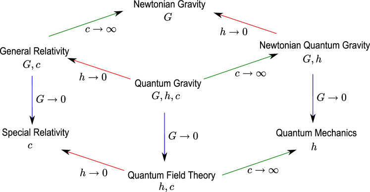
Figure 1: Quantum gravity merges quantum field theory and general relativity. As we take limits of $G\rightarrow 0$, $h\rightarrow 0$, or $c\rightarrow\infty$, we arrive at theories that are less complete with limited validity. A similar figure appeared in [17].

String theory is a candidate for the ultimate theory of quantum gravity. String theory can accommodate all the physical interactions, and having gravity is an inevitable consequence of string theory. Although the Universe appears to have three spatial dimensions and one temporal dimension, string theory predicts the existence of ten or more dimensions. Although this first appears paradoxical, these extra dimensions can be seen as tools. Much as gravity is explained as the curvature of spacetime, one hopes that the particle physics may be explained in terms of the geometry of these extra dimensions (as in Chapter 4, for example).

Furthermore, going to higher dimensions may resolve singularities. For example, the roller coaster has a smooth track in 3D, but its shadow on the ground, a 2D projection of 3D object, may show cusps, geometric singularities. Going to higher dimensions can resolve these artificial singularities in mathematics [18], and the same thing could happen in physics as well. Note that physics is not mathematics, but often can be efficiently described in terms of geometry; historically, geometric thinking actually accelerated the development of physics. For example, the way in which heavy objects curve the spacetime fabric in general relativity is best phrased in terms of Riemann geometry.

In quantum field theories, we come across singular behaviors. Scattering amplitudes for particle interactions are systematically organized in terms of Feynman diagrams. At the points of interaction, sharp singular behavior can occur in the scattering amplitude. In string theory we replace Feynman diagrams with pants diagrams, where each point particle is now replaced by a string, as in Figure 2. In string theory, there is not one single point of interaction: instead, it is smeared out over the smooth surface. Depending on how we choose our time coordinate, or depending on how fast we travel relative to a given reference frame, the interaction will appear to happen at different points. Nothing singles out a point in a pants diagram of string interaction. String theory fattens the thin Feynman diagrams into thick pants diagrams, removing the singularities at interaction vertices. Notions of “here” and “now” are spread out in string theory.

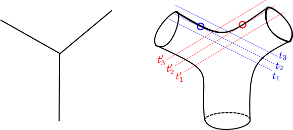
Figure 2: A Feynman diagram of an interaction among three fields on the left, and a “pants diagram” on the right, which depicts a process where three closed string states interact. Different Lorentz observers with time coordinates $t$ and $t^{\prime}$, will have different interaction points (marked with circles).

There is a price we have to pay to accept string theory as an avenue toward the Theory of Everything. For its own consistency, string theory, also called superstring theory, demands supersymmetry, while our world is not supersymmetric. However, there is no contradiction in describing the world by a theory whose general laws are symmetric, but whose solutions (vacua) are not. Also note that having supersymmetry in theory is very attractive. Supersymmetry unifies the coupling constants of gauge interactions - strong and weak nuclear forces and electromagnetic force. Supersymmetry is also helpful in solving the Higgs mass hierarchy problem, and it may provide dark matter candidates. Therefore, let us take the stance of starting from a supersymmetric theory and breaking supersymmetry to find a realistic non-supersymmetric vacuum in which we live. When symmetry is broken in a solution (vacuum) of a symmetric theory, we call that the symmetry is broken spontaneously in that vacuum.

Therefore, we still deal with supersymmetric string theory, but we will look for non-supersymmetric vacua where supersymmetry is spontaneously broken. More specifically, we want our vacua to have lifetimes long enough to allow our history of the Universe to fit in. Therefore, we want to find non-supersymmetric vacua that are exactly stable (with infinite lifetimes) or metastable (with finite lifetimes).

Breaking supersymmetry is only the tip of the iceberg of the string theory to-do list. We need to find a string theory vacuum that explicitly displays the particle properties of our Universe. Allowing certain interactions is not enough: we also want to be able to explain why each particle has certain properties, such as mass. This is a very active field of research in string theory, called string phenomenology, because it aims to explain particle or astrophysical phenomenology in string theory framework. Supersymmetry breaking in string theory and string phenomenology are intertwined problems, because the way we break supersymmetry affects the kinds of particle physics we get.

Among all the particles in the Standard Model of particle physics, neutrinos are particularly interesting. In the Standard Cosmology, neutrinos are also believed to be the most abundant particles in the Universe after photons. Neutrinos are much lighter than the other massive particles in the Standard Model, and they behave in very strange ways, such as changing their flavor with time, as is quantitatively captured in a neutrino mixing matrix. Neutrinos were thought to be massless until the 1970s, when flavor oscillations were observed in neutrinos arriving from the Sun. The only way to explain neutrino oscillation is to ascribe different masses to neutrinos, one for each flavor composition.

Constructing a string phenomenology model for neutrinos is a challenging but rewarding task. The principle difficulty is that relatively little experimental data is available: their masses have a large range of uncertainty, and it is unknown whether neutrinos are anti-particles of themselves (Majorana particles). However, they provide a window into physics beyond the Standard Model of particle physics, allowing us opportunities to make predictions for coming experiments.

1 Supersymmetry

Supersymmetry is the symmetry between fermions and bosons. Each elementary particle has a quantum number called spin, which has the same unit as angular momentum. Bosons have integer spin, and they like to clump together into the same quantum state. Fermions have half-integer spin, and they are mutually exclusive. For example, photons are bosons with spin one, and they stay together in the same state to form a strong coherent light in a laser. On the other hand, electrons are fermions with spin of a half, and (as explained by Pauli’s exclusion principle) they cannot stay in the same quantum state: so they inhabit successive orbital shells in an atom, rather than all occupying the inner-most shell.

Supersymmetry pairs bosons and fermions into super-multiplets. They are superpartners of each other, and except for spin they share all properties, including mass and charge. If the superpartners have different masses, this difference (mass splitting) denotes the amount of supersymmetry breaking in a vacuum. If we lived in a supersymmetric vacuum, we would see a massless photino, a superpartner to massless photon, and a light selectron, a bosonic superpartner to a light electron. Since none of these have been observed, clearly we live in a non-supersymmetric vacuum and superpartners are too heavy to be observed at the current energy scale of experiments.

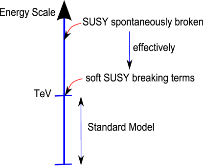
Figure 3: Spontaneous breaking of supersymmetry in a UV-complete theory gives soft SUSY breaking terms at the TeV scale for a Lagrangian of a low energy effective theory.

Currently, the most popular supersymmetry breaking scenario posits that we live in a supersymmetric, visible sector, and supersymmetry breaking happens spontaneously in hidden sectors at high energy, for example in string theory. There are messenger fields that mediate between visible and hidden sectors. The messenger’s supersymmetry is broken by interactions with fields in hidden sectors. The interaction terms between visible and messenger sectors will provide explicit soft supersymmetry breaking terms in the effective theory in the visible sector. As drawn in Figure 3, spontaneous breaking of supersymmetry at high energy provides an explicit supersymmetry breaking terms in the Lagrangian of the corresponding low energy effective theory. This makes the low energy effective theory appear as a non-supersymmetric theory with added explicit supersymmetry breaking terms with soft UV behavior. Chapters 1, 2, and 3 explore various ways of breaking supersymmetry in string theory.

2 Closed and open strings, and D-branes

In string theory, we have open and closed strings: open strings are like a path with 2 ends, and closed strings are like loops with no free ends. They have a topology of a line segment and a circle, respectively. Open strings have two endpoints, which must reside on multi-dimensional objects called D-branes, whereas closed strings can float around anywhere they like. To explain these concepts by analogy: imagine we fly airplanes. We could circle around in the sky, making a closed loop just like a closed string. If we fly from one airport to the other, then our flight path is an open string. The airport corresponds to D-branes where the flight path has to end or start: we cannot land anywhere we like, we can only land where this is an airport.

Dirichlet (D)-brane is a set of points where open strings can end. D-branes can come in many dimensions. D-branes and strings have tension energy proportional to their volume. Due to the brane tension energy, a D-brane tries to minimize its volume, like a rubber band wrapped on the stem of a wine glass. D-branes with opposite charges are called anti-D-branes. D-branes and anti-D-branes are attracted to each other, and they annihilate each other when brought together, like matter and anti-matter.

3 Intersection and wrapping of D-brane stacks

We can stack multiple D-branes at a same location. If we have two stacks of D-branes, an open string can stretch between them with one endpoint living on each stack. The mass (tension energy) of the open string is proportional to its length, i.e. or the separation between the stacks. As we bring the brane stacks closer, the string get shorter and the string mode become lighter. When we intersect the D-branes, near the intersection locus, we have matter fields which are light, easily excitable, string modes. When many stacks intersect at a point, we will have many fields, which are so close to one another that they can interact with one another, forming Yukawa interaction terms.

For our neutrino model in Chapter 4, matter fields arise along the curve where two stacks of D-branes intersect. Interaction terms between matter fields (Yukawa couplings) arise where these curves or stacks of D-branes intersect at a point.

D-branes and anti-D-branes break different halves of supersymmetry, together they break all supersymmetry. If put together in a flat geometry, they also attract and mutually annihilate. On open strings stretched between these two stacks of branes, dangerous tachyonic modes will be excited, which correspond to fluctuations which breaks down the vacuum. However, if two stacks are wrapped on different cycles that are far apart, with a barrier between them, then the system will become stable. A topological barrier gives exact stability we explore in Chapters 1 and 3, while a geometric barrier gives metastability we study in Chapters 2 and 3.

2 String dualities and D-branes

There are many string theories, which are related to each other by dualities. See the Figure 4 of string theory duality map. Start from type IIA, IIB, and I string theories, and then we discuss dualities, through which we arrive at other known string theories.

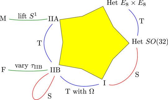
Figure 4: The map of dualities between string theories. S and T in the figure stand for strong-weak and toroidal dualities.

Type IIA, IIB, and I string theories are 10 dimensional The numbers I and II refer to the amount of supercharges seen in 10D. They have open strings which end on D-branes. Strings and branes can carry Neveu-Schwarz (NS) and Ramond (RR) charges. These charges are conserved: when geometry removes D-branes, RR-flux has to appear to replace their effect. More details are discussed in Chapters 2 and 3. A varying NS-field appears in Chapter 3 and provides exactly stable supersymmetry breaking vacua.

Type IIA and IIB string theories have left-and right-movers with opposite and equal chiralities. Type I string theory is obtained by identifying the left- and right-moving modes of type IIB string theory, and therefore it has less supersymmetry and no orientation. Type IIA and IIB string theories are related by toroidal (T) duality. T-duality interchanges the big and small radii on a torus, and changes the dimensions of D-branes by 1. Type IIB string theory is T-dual to type I string theory with the action of a worldsheet parity orientifold operator $\Omega$, which removes orientations of type IIB string theory which are already absent in type I string theory.

Strong-weak (S) duality interchanges strong and weak coupling constants. Inverting the coupling constant of type I string theory, one obtains $SO(32)$ heterotic string theory [19, 20]. Heterotic string theory has no open strings or D-branes. Instead, it has closed strings with left- and right-movers, which are bosonic (26d) and supersymmetric (10d) respectively. The extra 16 dimensions of a bosonic left-mover should have the structure of $E_{8}\times E_{8}$ or $SO(32)$ for the consistency. They correspond to $E_{8}\times E_{8}$ and $SO(32)$ heterotic string theories, which are T-dual to each other [21]. Heterotic string theory will appear in Chapter 1, which studies stability of its non-supersymmetric states.

Type IIB string theory is self-dual under S-duality. This strange behavior of the coupling constant of type IIB string theory leads to F-theory, a non-perturbative version of type IIB string theory in which the coupling constant $\tau_{\mathrm{I}IB}$ is allowed to vary, taking a value in a 2-torus. F-theory is discussed in Chapter 4, which constructs a model for neutrino physics.

M-theory is an 11-dimensional supergravity with no strings or branes. If compactified on a tiny circle, it becomes type IIA string theory.

There are other dualities not shown here. For example, heterotic string on $T^{4}$ is S-dual to type IIA string theory on K3 surface [20, 14], a fact which will be used in Chapter 1. Note that the amount of supersymmetry between these two theories matches because K3 surface kills half of the supersymmetry present, due to its holonomy.

3 Toward a realistic string phenomenology

This section is a concise introduction to various concepts necessary for constructing realistic particle theory models in string theory, focussing on supersymmetry breaking. More details discussions can be found in [22, 23, 24, 25].

If supersymmetry is broken spontaneously in the low energy theory at the leading order (at the tree level with no quantum corrections), the predicted masses of superpartners [26] are in contradiction with observations. Therefore the supersymmetry breaking needs to be explicit at low energy, with explicit supersymmetry breaking terms in the Lagrangian whose origin is quantum. However, in order to provide the Higgs mass with a soft UV behavior, supersymmetry breaking has to be spontaneous in a UV-complete theory, such as string theory. (See Figure 3.) In order to have a realistic Grand Unified Theory with chiral fermions, there is a further constraint for the theory to have only ${\mathcal{N}}=1$ supersymmetry at low energy [27].

The Minimally Supersymmetric Standard Model (MSSM) is a ${\mathcal{N}}=1$ version of the Standard Model. The MSSM lives in a visible sector, and supersymmetry breaks spontaneously in a hidden sector, usually at a UV complete theory such as string theory. Supersymmetry breaking at a hidden sector is mediated through messengers to MSSM at the visible sector. The interaction terms between the MSSM and the messengers provide the explicit supersymmetry breaking terms in the low energy Lagrangian. See [25] for a review of various mediation mechanisms.

The Higgsino attains a mass in the MSSM through an operator of the form

$${\mathcal{L}}=\int d^{2}\theta\mu H_{u}H_{d}+h.c..$$ (1)

A mass $\mu$ on the order of $100$ GeV roughly explains the weak scale. Explaining why $\mu$ takes this small value, which is near the soft SUSY breaking parameter, is the so-called “$\mu$ problem.”

The Giudice-Masiero mechanism [28] solves this problem by imposing a $U(1)$ Peccei-Quinn (PQ) symmetry and introducing messenger fields which mediate supersymmetry breaking. One starts by assigning PQ charges on Higgs fields $H_{u}$ and $H_{d}$ so that there will be no term of the form (1) in the leading order. The messenger field $X$ has the F-term vacuum expectation value $\langle X\rangle=x+\theta^{2}F_{X}$ with $F_{X}\neq 0$, providing a term like (1) in the subleading order. Therefore, PQ symmetry and messenger field $X$ together suppress the Higgsino mass. They suppress neutrino masses in Chapter 4, in agreement with the experimental results.

4 Organization of the thesis

Chapter 1 studies non-BPS objects in heterotic string theory and their stability region. In Chapters 2 and 3 discuss supersymmetry breaking mechanisms which maintain meta- or exact stability in type IIB string theory on a non-compact Calabi-Yau three-fold. Chapter 4 discusses a Grand Unified Theory model in F-theory, where the supersymmetry breaking mechanism provides the neutrino mass scale.

Chapter 1 Stability of non-BPS states in heterotic string theory

Exactly stable non-BPS states have been studied in various string theories, and they may help us to describe non-supersymmetric field theories and to construct non-supersymmetric string compactification [29, 30]. A non-BPS D0-brane is stable in type I string theory [31, 32, 33], which is realized as a stable non-BPS pair of a D1-brane and an anti-D1-brane in type IIA string theory [34]. This stability holds in a particular region of moduli space. At the boundary of the stability region, tachyons become massless, the force between non-BPS objects vanishes, and there is exact degeneracy in the Bose-Fermi spectrum [35, 36]. Non-BPS states and their stability against certain decay channels have been discussed for type IIA string theory compactified over a K3 surface [37] and a Calabi-Yau three-fold [38]. There are also stable non-BPS brane-antibrane constructions in type IIB string theory using D4-branes and anti-D4-branes hung between NS5-branes [39, 30]. See these review papers [29, 40, 41] on stable non-BPS string states.

We study stability of non-BPS states in heterotic string theory compactified on $T^{4}$ and map them to the dual type IIB theory on K3 surface as in [42, 41]. We systematically exhaust all the possible decay channels allowed by charge conservation, and then we find that a certain spinor representation has a large stability region, which contains those of other less stable non-BPS states as well. We interpret these non-BPS and BPS heterotic string states in terms of D-branes wrapped over orbifold limit of K3 surface in type IIA string theory.

We introduce a set of transformation matrices in heterotic string side, which is equivalent to taking even number of T-dualities on $T^{4}$. These $16\times 16$ matrices form a subgroup of isometry group of compactified 16 dimensional momentum vector of the left-mover of a heterotic string state. The momentum is a conserved charge and limits possible decay modes. With these new tools, one can study possible decay channels of given non-BPS states in a systematic way.

Stability region of non-BPS states in heterotic string theory turns out to be large. Every other corner of moduli space allows stable non-BPS states, and these corners are connected into one huge region of the moduli space where a non-BPS is stable against all the possible decays allowed by charge conservation. This may be a fertile path for studying non-supersymmetric field theory and supersymmetry-breaking hidden sectors for realistic model building in string theory.

The organization of the rest of the chapter is as follows. Section 1 reviews heterotic string theory and the duality chain between heterotic string theory and type IIA string theory. Section 2 introduces a new tool to keep track of conserved charges in heterotic string and analyze various non-BPS and BPS states in heterotic string using this tool. The stability region of non-BPS states is discussed in section 3

1 Heterotic string theory on $T^{4}$ and string-string duality

The section reviews heterotic string theory on $T^{4}$ and type IIA string theory on an orbifold limit of a K3 surface and discusses the duality chain between them.

1 Heterotic string theory on $T^{4}$

Heterotic string theory has a fermionic 10-dimensional right-mover and a bosonic 26-dimensional left-mover. The left-mover has extra 16 dimensions, whose momentum is quantized as a 16-dimensional vector ${P}_{L}=V_{K}\in\Gamma^{16}$. A 16-dimensional even self-dual lattice $\Gamma^{16}$ is given as

$$\Gamma^{16}=\left\{(n_{1},\cdots,n_{16}),\left(n_{1}+\frac{1}{2},\cdots,n_{16}+\frac{1}{2}\right)\bigg{|}\sum_{i}n_{i}\in 2\mathbb{Z}\right\}.$$ (1)

Heterotic string compactified on a 4-torus [43, 44] has Kaluza-Klein and winding excitations $n^{i},w_{i}\in\mathbb{Z}$ in each direction $x_{i}$ ($i=1,2,3,4$) of a 4-torus $T^{4}$. We also choose four Wilson lines $A^{i}$ (superscripts on the right-hand-side denoting repetition of components):

$$A^{1} = \left(\left(\frac{1}{2}\right)^{8},0^{8}\right),\qquad A^{2}=\left(\left(\left(\frac{1}{2}\right)^{4},0^{4}\right)^{2}\right)$$ (2)

$$A^{3} = \left(\left(\left(\frac{1}{2}\right)^{2},0^{2}\right)^{4}\right),\qquad A^{4}=\left(\left(\frac{1}{2},0\right)^{8}\right),$$ (3)

so that this heterotic string theory is dual to type IIA string theory compactified on an orbifold limit of a K3 surface. Now the left- and right-moving momenta in internal directions are given by

$$\mathbf{P}_{L}=(P_{L},p_{L}),\qquad\mathbf{P}_{R}=p_{R}.$$ (4)

The momentum of the left-mover on 16-dimensional lattice

$$P_{L}=V_{K}+A_{K}^{i}w_{i}$$ (5)

is shifted by Wilson lines and winding, where summation over $i=1,2,3,4$ is implied. Components for left- and right-moving momenta in $T^{4}$ are given as:

$$p_{L}^{i}=\frac{p^{i}}{2R_{i}}+w^{i}R_{i},\qquad p_{R}^{i}=\frac{p^{i}}{2R_{i}}-w^{i}R_{i},$$ (6)

where the index $i=1,2,3,4$ is not contracted. The physical momentum $p^{i}$ in the $T^{4}$ is also shifted by winding excitations and choice of Wilson lines as

$$p^{i}=n^{i}+B^{ij}w_{j}-V^{K}A^{i}_{K}-\frac{1}{2}A^{i}_{K}A^{j}_{K}w_{j},$$ (7)

with $w_{i},n_{i}\in{\mathbb{Z}}$ and contraction over the index $j=1,2,3,4$. For simplicity, we will assume $B^{ij}=0$ here.

The level matching condition has to be satisfied by any heterotic string state:

$${\frac{1}{2}}P_{L}^{2}+N_{L}-1={\frac{1}{2}}P_{R}^{2}+N_{R}-C_{R},$$ (8)

with

$$C_{R}=\frac{1}{2},\ \ {\mathrm{(}NS)};\qquad C_{R}=0,\ \ {\mathrm{(}R)}$$ (9)

for Neveu-Schwarz and Ramond sectors, respectively. Non-negative integers $N_{L}$ and $N_{R}-C_{R}$ denote oscillation numbers on the bosonic left-mover and the fermionic right-mover, respectively.

The BPS states with

$$N_{R}=C_{R}$$ (10)

saturate BPS bound, and half BPS (resp. quarter BPS) states form a short (resp. ultrashort) multiplet and satisfy $N_{L}=1$ (resp. $N_{L}=0$). The heterotic string state has mass given by:

$$\frac{1}{8}m_{h}^{2}={\frac{1}{2}}P_{L}^{2}+N_{L}-1={\frac{1}{2}}P_{R}^{2}+N_{R}-C_{R}.$$ (11)

2 A duality chain between heterotic theory and type IIA string theory

Type IIA string theory on an orbifold limit of a K3 surface is dual to heterotic string theory on $T^{4}$ [20, 14], through the following chain of dualities [42]

$$\frac{\mbox{het}}{T^{4}}\;\;\overset{S}{\longrightarrow}\frac{\mbox{I}\;}{T^{4}}\;\overset{T^{4}}{\longrightarrow}\frac{\mbox{IIB}\;}{T^{4}/{\mathsf{Z\!\!Z}}_{2}^{\prime}}\;\overset{S}{\longrightarrow}\frac{\mbox{IIB}\;}{T^{4}/{\mathsf{Z\!\!Z}}_{2}^{\prime\prime}}\;\overset{T}{\longrightarrow}\frac{\mbox{IIA}\;}{T^{4}/{\mathsf{Z\!\!Z}}_{2}}\;\,.$$ (12)

Here the $\mathbb{Z}_{2}$ actions are given as

$${\mathsf{Z\!\!Z}}_{2}^{\prime}=(1,\Omega\mathcal{I}_{4}),\qquad{\mathsf{Z\!\!Z}}_{2}^{\prime\prime}=(1,(-1)^{F_{L}}\mathcal{I}_{4}),\qquad{\mathsf{Z\!\!Z}}_{2}=(1,\mathcal{I}_{4}),$$ (13)

where the operator $\Omega$ reverses world-sheet parity and $F_{L}$ is the left-moving part of the spacetime fermion number. The operator $\mathcal{I}_{4}$ implements reflection in all 4 compact directions $x_{i}$’s of a 4-torus

$$\mathcal{I}_{4}:(x_{1},x_{2},x_{3},x_{4})\rightarrow(-x_{1},-x_{2},-x_{3},-x_{4}).$$ (14)

Since orbifolding in each direction gives 2 fixed points, the action of $\mathcal{I}_{4}$ on a 4-torus gives $2^{4}=16$ fixed points on an orbifold limit of a K3 surface.

This chain employs S-duality between type I and heterotic string theories, self-S-duality of type IIB string theory, T-duality between type I and IIB string theories along all four $x_{i}$ directions of $T^{4}$, and T-duality between type IIB and IIA string theories along $x_{4}$ direction.

Assuming a diagonal metric tensor for $T^{4}$, the coupling constant $g_{h}$ of heterotic string theory and the radii $R_{hi}$’s of $T^{4}$ are written in terms of the coupling constant $g_{A}$ of type IIA string theory and the moduli $R_{Ai}$’s of an orbifold limit of a K3 surface as [42]

$$g_{h}=\frac{V_{A}}{8g_{A}R_{A4}},\qquad R_{hj}={\frac{1}{2}}\frac{\sqrt{V_{A}}}{R_{Aj}R_{A4}},\qquad R_{h4}=\frac{\sqrt{V_{A}}}{2},$$ (15)

with

$$V_{A}\equiv R_{A1}R_{A2}R_{A3}R_{A4},\qquad V_{h}\equiv R_{h1}R_{h2}R_{h3}R_{h4}.$$ (16)

Radii along $x_{j}$ ($j=1,2,3$) directions and $x_{4}$ direction have different formula in (15) due to an extra T-duality along $x_{4}$ direction between type IIA and IIB string theories in the duality chain of (12). The masses of BPS states in type IIA and heterotic string theories are related to each other by [42]

$$m_{h}=\frac{\sqrt{V_{h}}}{g_{h}}m_{A}.$$ (17)

Table 1: Mappings between BPS states in heterotic and type IIA string theories. First two columns correspond to $p_{L}$ and $P_{L}$ of heterotic string states. Superscripts for $P_{L}$ denote repetition of components. A symbol $W_{i}$ denotes a set of these BPS objects with $w^{i}=1$ and $w^{j}=p=0$. Similarly, a set $M_{i}$ consists of the BPS excitation modes with minimal physical momentum $p^{i}=\frac{1}{2}$ in one of $T^{4}$ directions, with no other excitations $p^{j}=w=0$. The BPS heterotic string states are dual to BPS D-branes in type IIA string theory. The last column denotes the directions of cycles on which D-branes are wrapping.

$p_{L}$	$P_{L}$	symbol	K3 cycle
$\left(R_{h1},0,0,0\right)$	$\left((\pm{\frac{1}{2}})^{8},0^{8}\right){\mathrm{o}r}\left(0^{8},(\pm{\frac{1}{2}})^{8}\right)$	$W_{1}$	$x_{2},x_{3}$
$\left(0,R_{h2},0,0\right)$	$\left(\left((\pm\frac{1}{2})^{4},0^{4}\right)^{2}\right){\mathrm{o}r}\left(\left(0^{4},(\pm{\frac{1}{2}})^{4}\right)^{2}\right)$	$W_{2}$	$x_{1},x_{3}$
$\left(0,0,R_{h3},0\right)$	$\left(\left((\pm\frac{1}{2})^{2},0^{2}\right)^{4}\right){\mathrm{o}r}\left(\left(0^{2},(\pm{\frac{1}{2}})^{2}\right)^{4}\right)$	$W_{3}$	$x_{1},x_{2}$
$\left(0,0,0,R_{h4}\right)$	$\left((\pm{\frac{1}{2}},0)^{8}\right){\mathrm{o}r}\left((0,\pm{\frac{1}{2}})^{8}\right)$	$W_{4}$	$x_{1},x_{2},x_{3},x_{4}$
$\left(\frac{1}{4R_{h1}},0,0,0\right)$	$\left(0^{a},\pm 1,0^{7},\pm 1,0^{7-a}\right)$	$M_{1}$	$x_{1},x_{4}$
$\left(0,\frac{1}{4R_{h2}},0,0\right)$	$(0^{a},\pm 1,0^{3},\pm 1,0^{11-a})$	$M_{2}$	$x_{2},x_{4}$
$\left(0,0,\frac{1}{4R_{h3}},0\right)$	$(0^{a},\pm 1,0,\pm 1,0^{13-a})$	$M_{3}$	$x_{3},x_{4}$
$\left(0,0,0,\frac{1}{4R_{h4}}\right)$	$\left(0^{2a},\pm 1,\pm 1,0^{14-2a}\right)$	$M_{4}$	fixed point
$\left(0,0,0,\frac{1}{2R_{h4}}\right)$	$0^{16}$	$b$	bulk

3 Type IIA string theory compactified on an orbifold limit of a K3 surface

Consider compactification of type IIA string theory on an orbifold limit of a K3 surface, $T^{4}/{{\mathsf{Z\!\!Z}}_{2}}$. See [12] for a review. D-even-branes are BPS states in type IIA string theory, and their masses may be expressed as the tension $\frac{1}{g_{A}}$ times the volume of D-brane

$$m_{{\mathrm{B}PS},A}=\frac{{\mathrm{v}olume}}{g_{A}}.$$ (18)

A bulk D0-brane has a unit volume in 0-dimension and has the mass of $\frac{1}{g_{A}}$. Fractional D0-branes sit at the 16 fixed points of an orbifold limit of a K3 surface. After blowing up each fixed point into a 2-sphere, we can wrap D2-branes over these 2-cycles. The fractional D0-brane can be thought of as a D2-brane wrapping a vanishing 2-cycle, which comes from a resolution of an orbifold singularity. Fractional D0-branes have one-half unit volume in 0-dimension because of the ${\mathsf{Z\!\!Z}}_{2}$ orbifolding in the K3 surface. Their mass is $\frac{1}{2g_{A}}$, which is half of that of a bulk D0-brane. A D4-brane wrapping the whole K3 surface has mass $\frac{V_{A}}{2g_{A}}$. D2-branes wrapping the torus $T^{2}$ in $x_{j}$ and $x_{k}$ directions have mass $\frac{R_{Aj}R_{Ak}}{2g_{A}}$.

By matching the charges and the masses, Table 1 lists mappings between BPS states in heterotic and type IIA string theories. The first two columns correspond to $p_{L}$ and $P_{L}$ of heterotic string states, and symbols $W_{i}$ and $M_{i}$ in the third column denote BPS modes with minimum winding and momentum in $x_{i}$ direction, respectively. Reading off from $p_{L}$, left-moving momentum in $T_{4}$, the first 4 rows correspond to BPS excitation modes with unit wrapping $w^{i}=1$ in one of $T^{4}$ directions, with no other excitations $w^{j}=p=0$. From (7), 16-dimensional momentum $P_{L}$ has 8 half-integer entries and 8 integer entries. Level matching (8) and BPS conditions (10) further restrict $P_{L}$ to have eight zeros and eight $\pm\frac{1}{2}$’s. In order to satisfy (7), the signs before each $\pm\frac{1}{2}$ are chosen such that $P_{L}A^{i}\in{\mathbb{Z}}$ and $P_{L}A^{j}\in{\mathbb{Z}}+\frac{1}{2}$ for $j\neq i$. A symbol $W_{i}$ denotes a set of these BPS objects with $w^{i}=1$ and $w^{j}=p=0$.

Similarly, the next 4 rows of table 1 correspond to BPS excitation modes with minimal physical momentum $p^{i}=\frac{1}{2}$ in one of $T^{4}$ directions, with no other excitations $p^{j}=w=0$, which belong to a set $M_{i}$. Their $P_{L}\in{\mathbb{Z}}^{16}$ has 14 zero entries and two $\pm 1$ entries. The location of two $\pm 1$ entries are chosen to satisfy (7): there are $2^{4-i}-1$ zeroes between two $\pm 1$ entries, in order to satisfy $P_{L}A^{i}\in{\mathbb{Z}}+\frac{1}{2}$ and $P_{L}A^{j}\in\mathbb{Z}$ for $j\neq i$. There are also BPS bound states of these objects having more than one of $M_{i}$ and $W_{i}$ excitations.

The BPS heterotic string states are dual to BPS D-branes in type IIA string theory. The last column of table 1 denotes the directions of cycles on which D-branes are wrapping. Heterotic states in $W_{4}$ and $M_{4}$ are dual to D4-branes and fractional D0-branes respectively, and heterotic states in $W_{j}$ and $M_{j}$ ($j=1,2,3$) are dual to D2-branes over 2-cycles over $x_{k},x_{l}$ ($\{j,k,l\}=\{1,2,3\}$) and $x_{j},x_{4}$ directions, respectively.

A non-BPS state may decay into a collection of $n$ BPS states

$${\mathrm{(}state)}_{\mathrm{n}on-BPS}\rightarrow\sum_{i=1}^{n}{\mathrm{(}state)}_{{\mathrm{B}PS},i}$$ (19)

subject to charge conservation and non-creation of mass

$$\mathbf{P}_{\mathrm{n}on-BPS} = \sum_{i=1}^{n}\mathbf{P}_{{\mathrm{B}PS},i}$$ (20)

$$m_{\mathrm{n}on-BPS} \geq \sum_{i=1}^{n}m_{{\mathrm{B}PS},i}.$$ (21)

Take the following strategy to test existence of an exactly stable non-BPS state:

1. Start with the lightest possible non-BPS state whose mass does not depend on the moduli of $T^{4}$.

2. Classify a collection of BPS states that holds (20) and identify the lightest possible collection of BPS states in each class.

3. Compare masses and find conditions on moduli which nullify (21) for every class of BPS states.

For example, start with a non-BPS state of $P_{L}\in\left({\mathbb{Z}}+\frac{1}{2}\right)^{16}$, then the BPS decay products must contain some state which carries half-integers in some of these 16 entries of $P_{L}$. The BPS-states in $M_{i}$’s have only integer entries in $P_{L}$. Therefore, the decay channel must contain some of $W_{i}$’s as in Figure 1. Consider a non-BPS state with $p_{L}=p_{R}=0$, $w=p=0$,

$$P_{L}=\left(\frac{1}{2},\frac{1}{2},\frac{1}{2},-\frac{1}{2};\left(\frac{1}{2},-\frac{1}{2},-\frac{1}{2},-\frac{1}{2}\right)^{2};-\frac{1}{2},-\frac{1}{2},-\frac{1}{2},\frac{1}{2}\right),$$ (22)

and mass $m_{h}=\sqrt{8({\frac{1}{2}}P_{L}^{2}-1)}=\sqrt{8}$. Its BPS-decay products must contain states with $W_{i}$ excitations. The lightest possible collection of BPS-decay products are a pair of $W_{i}$ objects as discussed [41], with total mass $2\times\sqrt{8({\frac{1}{2}}P_{R}^{2})}=4|P_{R}|=4{R_{hi}}$. No other decays are allowed because of the form of the $P_{L}\in\left({\mathbb{Z}}+\frac{1}{2}\right)^{16}$. The stability region for this against all the possible decays allowed by charge conservation is therefore a corner of moduli space with

$$\sqrt{8}<4{R_{hi}},\qquad i=1,2,3,4.$$ (23)

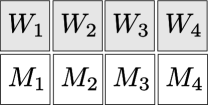
Figure 1: For a non-BPS state with $p_{R}=p_{L}=0$ and $P_{L}\in\left({\mathbb{Z}}+\frac{1}{2}\right)^{16}$, possible BPS-decay channels must contain one of the shaded objects, $W_{i}$’s here.

As discussed in [41], this non-BPS state in heterotic string theory corresponds to a non-BPS $\widehat{D3}$-brane in type IIA string theory stretched along $x_{1},x_{2},x_{3}$ directions. The symbol $\widehat{\phantom{D}}$ over $\widehat{D}$-brane denotes that a D-brane has wrong dimensions and is a non-BPS object. D-even-branes (D-odd-branes) are BPS (non-BPS) objects in type IIA string theory. The lightest possible BPS decay products are a pair of D4-brane and anti-D4-brane, or a pair of D2-brane and anti-D2-brane spanning $i$ and $j$ directions with $i,j\in\{1,2,3\}$.

This demonstrates restriction for decay modes of non-BPS states with $p_{R}=p_{L}=0$, $P_{L}=\left((\pm{\frac{1}{2}})^{16}\right)$ to contain some of $W_{i}$’s. Similarly, one may ask whether there are non-BPS objects whose decay products must contain some of $M_{i}$’s instead. This answer is yes, due to symmetry. The next section introduces a set of eight $16\times 16$ unitary matrices acting on $P_{L}$ and shows how charge conservation constrains possible decay modes into BPS states in a systematic way. For example, we will see that a similar constraint exists for a non-BPS object with $p_{R}=p_{L}=0$ and $P_{L}=\left(2,0^{15}\right)$, and its decay modes must contain some of $M_{i}$.

2 A systematic test of non-BPS stability

The transformations for 16-dimensional momentum vector $P_{L}$ of the left-mover of heterotic string states are given by the $16\times 16$ matrices ${\mathsf{1\!\!1}}_{16},T_{1234}$, and $T_{ij}$ with $i<j\in\{1,2,3,4\}$, given by the following formulas:

$$T_{12}\equiv\left(\begin{array}[]{cccc}L&0&0&0\\ 0&0&R&0\\ 0&R&0&0\\ 0&0&0&L\end{array}\right),$$ (24)

$$T_{13} \equiv U_{23}\cdot T_{12}\cdot U_{23},\qquad T_{14}\equiv U_{34}\cdot T_{13}\cdot U_{34}$$ (25)

$$T_{23} \equiv U_{12}\cdot T_{13}\cdot U_{12},\qquad T_{24}\equiv U_{34}\cdot T_{23}\cdot U_{34},\qquad T_{34}\equiv U_{23}\cdot T_{24}\cdot U_{23}$$ (26)

$$T_{1234} \equiv T_{12}\cdot T_{34}=T_{13}\cdot T_{24}=T_{14}\cdot T_{23},$$ (27)

where $L$ and $R$ are $4\times 4$ matrices given below:

$$L\equiv\left(\begin{array}[]{cccc}+{\frac{1}{2}}&+{\frac{1}{2}}&+{\frac{1}{2}}&-{\frac{1}{2}}\\ +{\frac{1}{2}}&+{\frac{1}{2}}&-{\frac{1}{2}}&+{\frac{1}{2}}\\ +{\frac{1}{2}}&-{\frac{1}{2}}&+{\frac{1}{2}}&+{\frac{1}{2}}\\ -{\frac{1}{2}}&+{\frac{1}{2}}&+{\frac{1}{2}}&+{\frac{1}{2}}\end{array}\right),\qquad R\equiv\left(\begin{array}[]{cccc}+{\frac{1}{2}}&-{\frac{1}{2}}&-{\frac{1}{2}}&-{\frac{1}{2}}\\ -{\frac{1}{2}}&+{\frac{1}{2}}&-{\frac{1}{2}}&-{\frac{1}{2}}\\ -{\frac{1}{2}}&-{\frac{1}{2}}&+{\frac{1}{2}}&-{\frac{1}{2}}\\ -{\frac{1}{2}}&-{\frac{1}{2}}&-{\frac{1}{2}}&+{\frac{1}{2}}\end{array}\right).$$ (28)

Each $16\times 16$ unitary matrix $U_{ij}$ exchanges $x_{i}$ and $x_{j}$ directions in $T^{4}$ and written as:

$$U_{12} \equiv \left(\begin{array}[]{cccc}{{\mathsf{1\!\!1}}}_{4}&0&0&0\\ 0&0&{\mathsf{1\!\!1}}_{4}&0\\ 0&{\mathsf{1\!\!1}}_{4}&0&0\\ 0&0&0&{\mathsf{1\!\!1}}_{4}\end{array}\right),$$ (33)

$$U_{23} \equiv \left(\begin{array}[]{cc}u_{23}&0\\ 0&u_{23}\end{array}\right),\qquad U_{34}\equiv\left(\begin{array}[]{cccc}u_{34}&0&0&0\\ 0&u_{34}&0&0\\ 0&0&u_{34}&0\\ 0&0&0&u_{34}\end{array}\right),$$ (40)

with following $8\times 8$ and $4\times 4$ submatrices:

$$u_{23}\equiv\left(\begin{array}[]{cccc}{\mathsf{1\!\!1}}_{2}&0&0&0\\ 0&0&{\mathsf{1\!\!1}}_{2}&0\\ 0&{\mathsf{1\!\!1}}_{2}&0&0\\ 0&0&0&{\mathsf{1\!\!1}}_{2}\end{array}\right),\qquad u_{34}\equiv\left(\begin{array}[]{cccc}1&0&0&0\\ 0&0&1&0\\ 0&1&0&0\\ 0&0&0&1\end{array}\right).$$ (41)

All of $T$’s commute with one another, and have unit determinant and squares to an identity matrix,

$$T_{1234}^{2}=T_{ij}^{2}={\mathsf{1\!\!1}}_{16},\qquad i<j\in\{1,2,3,4\}.$$ (42)

A transformation matrix $T_{ij}$ corresponds to T-dualities on $x_{i}$ and $x_{j}$ directions in $T^{4}$ and exchanges excitations in $W_{i,j}\rightarrow M_{i,j}$ classes. Similarly, $T_{1234}$ corresponds to T-dualities on all the four directions in $T^{4}$ and exchanges excitations in $W_{1,2,3,4}\rightarrow M_{1,2,3,4}$ classes.

Starting from a BPS object in $M_{4}$ class with $P_{L}=\left(1,1,0^{14}\right)$, one has

$$P_{L} = P_{L}\cdot T_{12}=P_{L}\cdot T_{13}=P_{L}\cdot T_{23}=\left(1,1,0^{14}\right)$$ (43)

$$P_{L}\cdot T_{1234} = P_{L}\cdot T_{14}=P_{L}\cdot T_{24}=P_{L}\cdot T_{34}$$ (44)

$$= \left(\frac{1}{2},0,\frac{1}{2},0;\frac{1}{2},0,-\frac{1}{2},0;\frac{1}{2},0,-\frac{1}{2},0;-\frac{1}{2},0,-\frac{1}{2},0\right).$$ (45)

The transformation by $T_{i4}$ or $T_{1234}$ turns $P_{L}$ of $M_{4}$ class into $P_{L}$ of $W_{4}$ class which has half-integer elements as seen in table 1.

Similarly, starting from a BPS object in $M_{1}$ class with $P_{L}=\left(1,0^{7},1,0^{7}\right)$, one has

$$P_{L} = P_{L}\cdot T_{23}=P_{L}\cdot T_{24}=P_{L}\cdot T_{34}=\left(1,0^{7},1,0^{7}\right)$$ (46)

$$P_{L}\cdot T_{1234} = P_{L}\cdot T_{12}=P_{L}\cdot T_{13}=P_{L}\cdot T_{14}$$ (47)

$$= \left(\frac{1}{2},\frac{1}{2},\frac{1}{2},-\frac{1}{2},\frac{1}{2},-\frac{1}{2},-\frac{1}{2},-\frac{1}{2},0^{8}\right).$$ (48)

The transformation by $T_{1j}$ or $T_{1234}$ turns $P_{L}$ of $M_{1}$ class into $P_{L}$ of $W_{1}$ class which has half-integer elements as seen in table 1.

One may conclude that for a BPS object, $T_{ij}$ will reverse the form of $P_{L}$ of $W_{a}\leftrightarrow M_{a}$ for $a=i,j$ and $T_{1234}$ will reverse the form of $P_{L}$ of $W_{a}\leftrightarrow M_{a}$ for $a=1,2,3,4$. The transformations induced on a BPS object are partially shown here:

$$P_{L}$$

.

(49)

Here $\leftrightarrow$ on the $i$’th row indicates that $W_{i}$ and $M_{i}$ exchange the form of their $P_{L}$ charges.

The transformation by $T_{1234}$ exchanges all $W_{i}\leftrightarrow M_{i}$. As promised earlier, we have now found a non-BPS state whose decay product now must contain some of $M_{i}$. A non-BPS state with $p_{R}=p_{L}=0$ and $P_{L}\cdot T_{1234}\in\left({\mathbb{Z}}+\frac{1}{2}\right)^{16}$ can decay only into sets of BPS states that contain some of $M_{i}$’s, as shown in Figure 2. For example, a non-BPS state with $p_{R}=p_{L}=0$ and

$$P_{L} = \left(2,0^{15}\right)$$ (50)

$$P_{L}\cdot T_{1234} = \left(\frac{1}{2},\frac{1}{2},\frac{1}{2},-\frac{1}{2};\left(\frac{1}{2},-\frac{1}{2},-\frac{1}{2},-\frac{1}{2}\right)^{2};-\frac{1}{2},-\frac{1}{2},-\frac{1}{2},\frac{1}{2}\right)$$ (51)

can decay into a brane-antibrane pair of any of $M_{1},M_{2},M_{3},M_{4}$ as in [42, 41], and we have shown that the lightest collection of BPS decay products must contain a pair of any of $M_{i}$’s. No other decays with less mass are possible. This non-BPS object is interpreted as a non-BPS $\widehat{D1}$-brane stretched along $x_{4}$ direction [42, 41]. The possible BPS decay products allowed by charge conservation are into a pair of wrapped D0-brane and anti-D0-brane, or a pair of D2-brane and anti-D2-brane spanning $x_{i}$ and $x_{4}$ directions with $i=1,2,3$. The mass of non-BPS state, before decay, is $\sqrt{8({\frac{1}{2}}P_{L}^{2}-1)}=\sqrt{8}$. The mass on the BPS side, after decay, is $2\times\sqrt{8({\frac{1}{2}}P_{R}^{2})}=4|P_{R}|=\frac{1}{R_{hi}}$ where $i=1,2,3,4$. The stability region for this object against every possible BPS decay is

$$\sqrt{8}<\frac{1}{R_{hi}},\qquad i=1,2,3,4$$ (52)

which holds in another corner of moduli space.

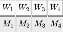
Figure 2: For a non-BPS state with $p_{R}=p_{L}=0$ and $P_{L}\cdot T_{1234}\in\left({\mathbb{Z}}+\frac{1}{2}\right)^{16}$, possible BPS-decay channels must contain one of the shaded objects, $M_{i}$’s here.

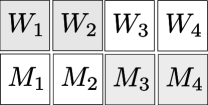
Figure 3: For a non-BPS state with $p_{R}=p_{L}=0$ and $P_{L}\cdot T_{34}\in\left({\mathbb{Z}}+\frac{1}{2}\right)^{16}$, possible BPS-decay channels must contain one of the shaded objects, $W_{1},W_{2},M_{3}$, and $M_{4}$ here.

Decay products of a non-BPS object with $p_{R}=p_{L}=0$ and

$$P_{L} = \left(1,1,1,-1,0^{12}\right),\qquad P_{L}\cdot T_{12}=\left(2,0^{15}\right)$$ (53)

$$P_{L}\cdot T_{34} = \left(\frac{1}{2},\frac{1}{2},\frac{1}{2},-\frac{1}{2};\left(\frac{1}{2},-\frac{1}{2},-\frac{1}{2},-\frac{1}{2}\right)^{2};-\frac{1}{2},-\frac{1}{2},-\frac{1}{2},\frac{1}{2}\right)$$ (54)

must contain some of $W_{1},W_{2},M_{3},M_{4}$ as in Figure 3. Similarly, BPS decay products of a non-BPS state with $p_{R}=p_{L}=0$ and $P_{L}\cdot T_{ij}=\left((\pm{\frac{1}{2}})^{16}\right)$ must contain some of $M_{i},M_{j},W_{k},W_{l}$ where $\{i,j,k,l\}=\{1,2,3,4\}$.

A non-BPS object with $p_{R}=p_{L}=0$ and $P_{L}\cdot T_{i4}=(0^{a},\pm 2,0^{b})$ has $P_{L}\cdot T_{jk}=((\pm{\frac{1}{2}})^{16})$ and the lightest possible BPS decay products must contain some of $M_{i},M_{4},W_{j},W_{k}$, which are D2-branes spanning $x_{i}$ and $x_{4}$ directions (where $l=1,2,3$) and D0-branes at fixed points of an orbifold limit of a K3 surface. Therefore, this corresponds to a non-BPS $\widehat{D1}$-brane, stretched along stretched along $x_{i}$ direction, with the non-BPS stability condition

$$\sqrt{8}<\frac{1}{R_{hi}},4{R_{hj}},4{R_{hk}},\frac{1}{R_{h4}},\qquad\{i,j,k\}=\{1,2,3\}.$$ (55)

Similarly, a non-BPS object with $p_{R}=p_{L}=0$ and $P_{L}\cdot T_{jk}=(0^{a},\pm 2,0^{b})$ has $P_{L}\cdot T_{i4}=((\pm{\frac{1}{2}})^{16})$ and the lightest possible BPS decay products must contain some of $W_{i},W_{4},M_{j},M_{k}$, which are D2-branes spanning $x_{j}$ and $x_{k}$ direction and D4-branes spanning all 4 directions. Therefore this corresponds to a non-BPS $\widehat{D3}$-brane, stretched along stretched along $x_{j},x_{k},x_{4}$ directions, with the non-BPS stability condition

$$\sqrt{8}<4{R_{hi}},\frac{1}{R_{hj}},\frac{1}{R_{hk}},4{R_{h4}},\qquad\{i,j,k\}=\{1,2,3\}.$$ (56)

The results from (23), (52), (55), and (56) can be summarized as follows: A stable non-BPS object exists in every other corner of moduli space, where even number of radii are small and the rest even number of radii are large. In the dark shades in Figure 4, one kind of non-BPS states we considered become exactly stable. In type IIA string theory, they correspond to non-BPS $\widehat{D1}$-branes and non-BPS $\widehat{D3}$-branes.

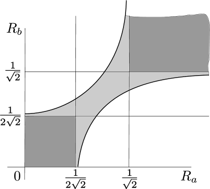
Figure 4: A non-BPS state of charge $P_{L}=\left(\left(\frac{1}{2}\right)^{16}\right)$ is stable in all the shaded regions. Drawn is a 2d slice varying two radii $R_{a}$ and $R_{b}$ of the $T^{4}$, fixing both of the other two radii $R_{c}$ and $R_{d}$ very large or small - namely $R_{c},R_{d}>\frac{1}{\sqrt{2}}$ or $R_{c},R_{d}<\frac{1}{2\sqrt{2}}$. If $R_{c}>\frac{1}{\sqrt{2}}$ and $R_{d}<\frac{1}{2\sqrt{2}}$, then it will roughly appear as shown, with one of the axis now denoting $\frac{1}{4R}$ instead of $R$. As we choose less extreme values for $R_{c}$ and $R_{d}$, the light shade will get larger.            An extra type of non-BPS states become exactly stable in the dark shades.

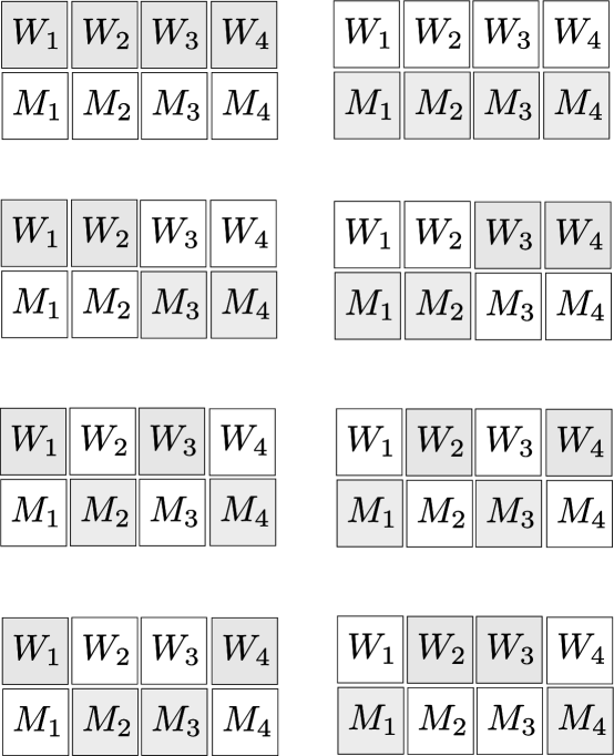
Figure 5: A non-BPS object with $p_{R}=p_{L}=0$ and $P_{L}\cdot M\in\left({\mathbb{Z}}+\frac{1}{2}\right)^{16}$ for all eight $T$’s can decay only into sets of BPS states that have overlap with all of these eight groups.

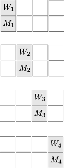
Figure 6: Charge allows a non-BPS state with $p_{R}=p_{L}=0$ and $P_{L}=\left(\left({\frac{1}{2}}\right)^{16}\right)$ to decay into $M_{a}$ and $W_{a}$ pairs with $a=1,2,3,4$, but energy prohibits those decays.

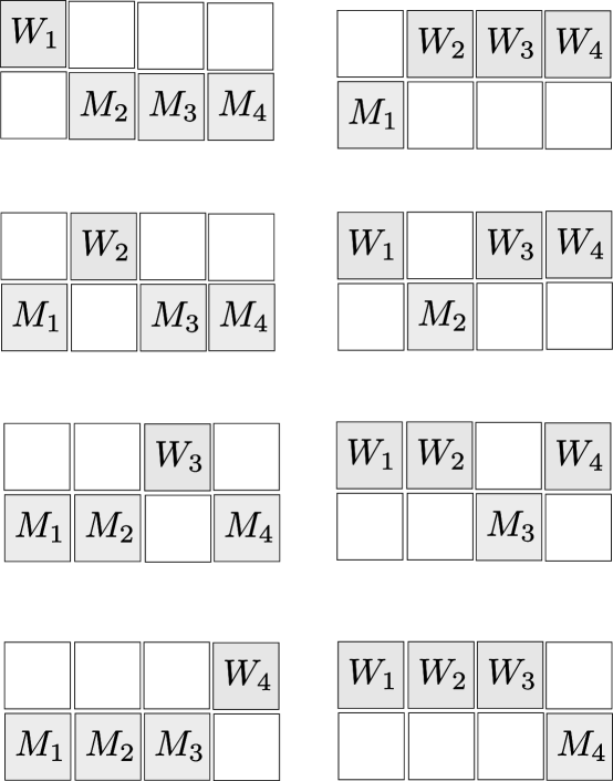
Figure 7: Charge allows a non-BPS state with $p_{R}=p_{L}=0$ and $P_{L}=\left(\left({\frac{1}{2}}\right)^{16}\right)$ to decay into $2(W_{a}+M_{b}+M_{c}+M_{d})$ or $2(W_{a}+W_{b}+W_{c}+M_{d})$ with $\left\{a,b,c,d\right\}=\left\{1,2,3,4\right\}$.

3 Stability region of a non-BPS state in heterotic string theory

In the previous section, we showed that the form of $P_{L}$ can restrict possible BPS-decay modes. To maximize this effect, we now study a non-BPS object with $P_{L}\cdot T\in\left({\mathbb{Z}}+\frac{1}{2}\right)^{16}$ for all the eight $T$’s. For example, a non-BPS state with $p_{R}=p_{L}=0$ and $P_{L}=\left(\left({\frac{1}{2}}\right)^{16}\right)$ satisfies $P_{L}\cdot T\in\left(\pm\frac{1}{2}\right)^{16}$ for all the eight $T$’s, and its decay products must have overlap with all of the these eight groups $\{W_{i}\},\{M_{i}\},\{M_{i},M_{j},W_{k},W_{l}\}$ with $\{i,j,k,l\}=\{1,2,3,4\}$ as depicted in Figure 5.

This severe restriction on decay channel comes from a ${{\mathbb{Z}}_{2}}^{8}$ parity, where each which ${{\mathbb{Z}}_{2}}$ determines whether $P_{L}\cdot T\in{\mathbb{Z}}^{16}$ or $P_{L}\cdot T\in\left({\mathbb{Z}}+\frac{1}{2}\right)^{16}$. This is reminiscent of ${{\mathbb{Z}}_{2}}$ symmetry of a SO(32) spinor representation of heterotic string theory in 10d, which does not decay due to conserved charge [45].

The lightest collections of BPS decay products are in following two kinds:

• $2(M_{a}+W_{a})$ as in Figure 6.

• $2(W_{a}+M_{b}+M_{c}+M_{d})$ or $2(W_{a}+W_{b}+W_{c}+M_{d})$ with $\left\{a,b,c,d\right\}=\left\{1,2,3,4\right\}$ as in Figure 7.

Mass on BPS side of the first kind

$$\frac{1}{R_{a}}+4R_{a}\geq 4>\sqrt{8}$$ (57)

is always heavier than the original non-BPS state, so this decay is excluded by energy. This set of heterotic BPS states are dual to two pairs of D-brane and anti-D-brane in type IIA string theory as following:

• a pair of D2-brane and anti-D2-brane over $x_{i},x_{j}$ and another pair over $x_{k},x_{l}$

• a pair of D0-brane and anti-D0-brane and a pair of D4-brane and anti-D4-brane.

The non-BPS brane in type IIA string theory may correspond to a bound state of a non-BPS $\widehat{D1}$-brane and $\widehat{D3}$-brane, which was studied in [41].

Masses of the second type of decay products sum up to

$$\left(16R_{a}^{2}+\frac{1}{R_{b}^{2}}+\frac{1}{R_{c}^{2}}+\frac{1}{R_{d}^{2}}\right)^{\frac{1}{2}}$$ (58)

$$\left(16R_{a}^{2}+16R_{b}^{2}+16R_{c}^{2}+\frac{1}{R_{d}^{2}}\right)^{\frac{1}{2}}$$ (59)

respectively. Therefore, this non-BPS object is exactly stable against decay into BPS states if and only if both of following hold:

$$16R_{a}^{2}+\frac{1}{R_{b}^{2}}+\frac{1}{R_{c}^{2}}+\frac{1}{R_{d}^{2}} > 8$$ (60)

$$16R_{a}^{2}+16R_{b}^{2}+16R_{c}^{2}+\frac{1}{R_{d}^{2}} > 8.$$ (61)

If we consider the moduli space of $T^{4}$ as a 4d cube, then among 16 corners, this non-BPS state will be exactly stable in alternate corners and in the connecting region between them. The stability region looks like 4d cheese in a shape of a cube with every other corner (where odd number of radii are large and odd number of radii are small) eaten. See Figures 4 and 8 for the 2d and 3d projection of stability region of this non-BPS state against decay into energetically competing BPS sides $2(W_{a}+M_{b}+M_{c}+M_{d})$ or $2(W_{a}+W_{b}+W_{c}+M_{d})$. Each of uneaten 8 corners (where even number of radii are large and even number of radii are small) corresponds to where we have one kind of exactly stable non-BPS heterotic string states, which corresponds to a non-BPS $\widehat{D}$-brane (a non-BPS $\widehat{D1}$-brane or a non-BPS $\widehat{D3}$-brane) each along 4 possible choices of directions.

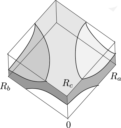
Figure 8: A non-BPS state of charge $P_{L}=\left(\left(\pm\frac{1}{2}\right)^{16}\right)$ is stable inside the shaded object, which looks like a cheese whose every other corner is eaten. Here we drawn a 3d slice of phase structure varying three radii $R_{a}$, $R_{b}$, $R_{c}$ of the $T^{4}$, fixing $R_{d}$ large, $R_{c},R_{d}>\frac{1}{\sqrt{2}}$.            If they instead chose $R_{d}<\frac{1}{2\sqrt{2}}$ to be small, then it will roughly look similar to this, with one of the axis denoting $\frac{1}{4R}$ instead of $R$. As we choose less extreme values for $R_{d}$, the stability region will get thicker.

The allowed modes $2(W_{4}+M_{i}+M_{j}+M_{k})$, $2(W_{i}+W_{j}+W_{k}+M_{4})$, $2(W_{i}+M_{j}+M_{k}+M_{4})$, and $2(W_{4}+W_{i}+W_{j}+M_{k})$ correspond to BPS bound states of D2-branes wrapped over $(x_{i},x_{l}),(x_{j},x_{l})$ and $(x_{k},x_{l})$ directions and a D4-brane wrapped over $x_{1},x_{2},x_{3},x_{4}$ directions, or BPS bound states of D2-branes over $(x_{i},x_{j}),(x_{j},x_{k}),(x_{i},x_{k})$ and a D0-brane.

A question remaining for future study is determination of the non-BPS stability region in type IIA string theory. Duality may not be a sufficient test of stability of non-BPS objects. For example, a non-BPS D0-brane is unstable in type IIB string theory, but stable in type I string theory [31, 32, 33] because the orientifold action projects out tachyon modes in type I [33].

Non-BPS states made of D-branes in ${{\mathbb{Z}}_{2}}\times{{\mathbb{Z}}_{2}}$ orientifolds with torsion are studied in [46]. The stability region is computed using boundary state formalism and demanding the tachyons to be massless [46]. The non-BPS stability region delineated by (60) and (61) has a similar shape to those computed in [46, 47]. In type IIA string theory, BPS D2-branes wrapped on 2-cycles of a Calabi-Yau 3-fold are studied, and a similar looking phase diagram appeared by considering decays between non-BPS $\widehat{D1}$-brane and non-BPS $\widehat{D3}$-brane [48].

Chapter 2 Metastable vacua of D5-branes and anti-D5-branes

Encouragement by the existence of metastable vacua are generic in supersymmetric gauge theories [49], we now construct metastable supersymmetry breaking vacua in string theory, as suggested in [50]. In this scenario, we wrap branes and anti-branes on cycles of local Calabi-Yau three-folds, yielding metastability as a consequence of the geometry. The branes and the anti-branes are wrapped over two separate rigid 2-cycles. The motion required for the branes to annihilate, costs energy, since the relevant minimal 2-spheres are rigid. This gives rise to a potential barrier, resulting in metastable configurations, as illustrated in Figure 1.

When the number of branes and anti-branes $N$ is large, the brane-antibrane metastable system has a dual description in a low energy effective theory. The dual description is obtained via a geometric transition in which the 2-spheres shrink, and are subsequently replaced by 3-spheres with fluxes through them. This flux spontaneously breaks the $\mathcal{N}=2$ supersymmetry to an $\mathcal{N}=1$ subgroup in the case that only branes are present. When only anti-branes are present, we expect supersymmetry to be broken to a different $\mathcal{N}=1$ subgroup. With both branes and anti-branes, the supersymmetry is completely broken $\mathcal{N}=0$. The vacuum structure can be analyzed from an effective potential. Unlike in the branes-only cases studied before, one expects to find a meta-stable vacuum which breaks supersymmetry completely.

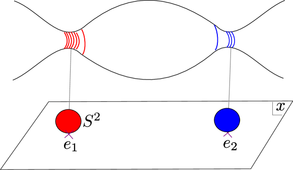
Figure 1: A metastable supersymmetry breaking system made of a stack of D-branes and another stack of anti-D-branes wrapped on 2-spheres which are rigid and separated.

Next, restrict further to the cases $N_{1}=-N_{2}$ and $\left|N_{1}\right|\gg\left|N_{2}\right|$ with the branch cuts aligned along the real axis of the complex $x$-plane. For sufficiently large ’t Hooft coupling, but far before the cuts touch, the theory undergoes a phase transition and decay occurs.

The organization of the rest of the chapter is as follows. Section 1 presents metastable configurations of brane and anti-branes. Section 2 computes the masses to the higher order to identify the decay modes. Section 3 studies the moduli space of 2-cut geometry.

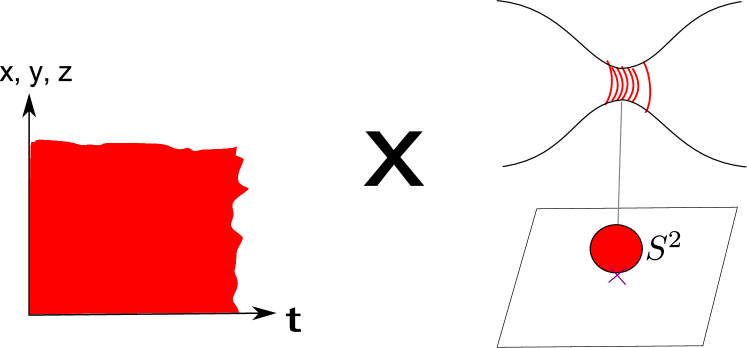
Figure 2: A stack of $N$ D5-branes fill spacetime and wrap a 2-cycle of internal Calabi-Yau three-fold.

1 Branes and anti-branes on the conifold

Consider type IIB string theory with $N$ D5-branes wrapping the $S^{2}$ of a resolved conifold in a local Calabi-Yau three-fold, and the remaining 3+1 dimensions filling the Minkowski spacetime. See Figure 2.

Type IIB string theory has $\mathcal{N}=2$ in 10-dimension. Compactifying string theory on a 6-dimensional manifold naively yields a theory in $d=4$ with $\mathcal{N}=8$. Choosing the 6-manifold to be a Calabi-Yau 3-fold breaks supersymmetry from $\mathcal{N}=8$ into $\mathcal{N}=2$, due to $SU(3)$ holonomy of a Calabi-Yau 3-fold. D-branes breaks one-half of $\mathcal{N}=2$ and preserves $\mathcal{N}=1$, while adding anti-branes preserves an orthogonal $\mathcal{N}=1$ subset. If we have multiple conifolds, then we can put a stack of D-branes on a local conifold, and a stack of anti-D-branes on some other, getting $\mathcal{N}=0$ system as in Figure 1.

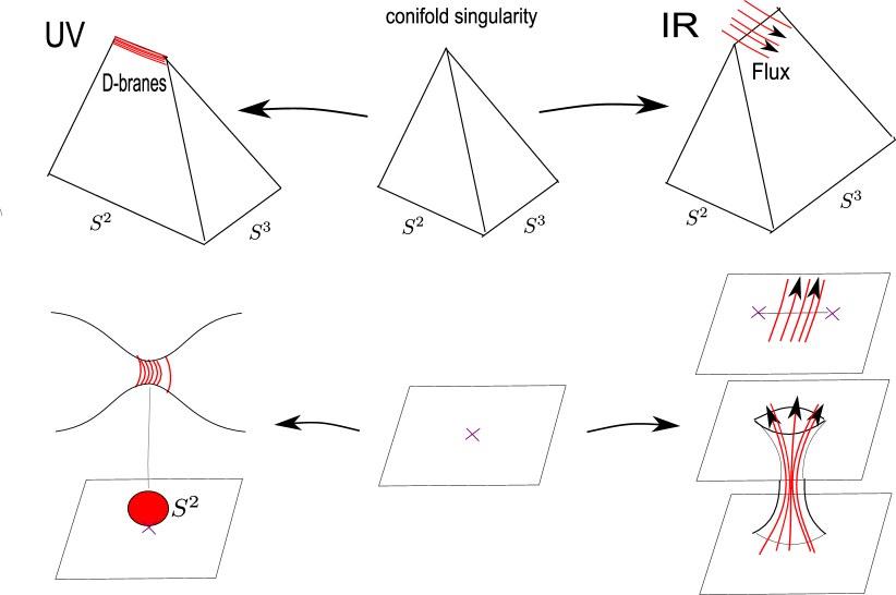
Figure 3: Blow-up (resolution) and complex deformation of a conifold singularity. In a UV theory, D-branes are wrapped over these non-vanishing $S^{2}$. One can also deform the singularity by complex deformation, which will now open up a new $S^{3}$ cycle through which RR-flux pierces in an IR theory.

These stacks of D-branes and anti-D-branes attract, as they try to annihilate each other. In order to meet, they have to increase their volume in $S^{2}$ directions in the Calabi-Yau geometry. This requires tension energy, which is proportional to the volume.

Guided by this qualitative understanding, we analyze this system in a low energy effective theory in a flux picture, where the branes are replaced by RR-flux. It is then straightforward to compute the effective potential, find its vacuum, and compute the masses and phase structure. Figure 3 shows how a conifold singularity is resolved in UV and IR pictures. One can resolve singularity by giving a size to a singular point of vanishing $S^{2}$. In a UV theory, D-branes are wrapped over these non-vanishing $S^{2}$. One can also deform the singularity by complex deformation, which will now open up a new $S^{3}$ cycle through which RR-flux pierces in an IR theory.

1 Local multi-critical geometry

Consider a Calabi-Yau three-fold given by

$${\ uv=y^{2}+W^{\prime 2}}$$ (1)

where

$$W^{\prime}(x)=g\prod_{k=1}^{n}(x-e_{k}).$$ (2)

There are $n$ isolated ${S^{2}}$’s at $x=e_{k}$ whose area is given as

$${A(x)=(|r|^{2}+\left|W^{\prime}\right|^{2})^{1/2}.}$$ (3)

The geometry in the $n=2$ case is drawn in Figure 4

Figure 4: We blow up conifold singularities by giving size $r$ to $S^{2}$.

Consider wrapping some number of branes $N_{k}$, $k=1,\cdots n$ on each ${S^{2}}$. The case when all the branes are D5-branes (with $N_{k}>0$ for all $k$) was studied in [51], giving an $\mathcal{N}=1$ supersymmetric $U(N)$ gauge theory on branes. The effective coupling constant $g_{\mathrm{YM}}$ of the four dimensional gauge theory living on the brane is the area of the minimal ${S^{2}}$’s times $1/g_{s}$:

$$\frac{1}{g_{\mathrm{YM}}^{2}}=\frac{|r|}{g_{s}}.$$ (4)

This chapter studies the case when some of the ${S^{2}}$’s are wrapped with D5-branes and others with anti-D5-branes. When the ${S^{2}}$’s are (or $e_{i}$ are) widely separated, the branes and the anti-branes are expected to interact weakly. However, the system should be only meta-stable because supersymmetry is broken and there are lower energy vacua available where some of the branes annihilate. For the branes to annihilate the anti-branes, they have to climb the potential as in Figure 1. We have thus geometrically engineered a metastable brane-antibrane configuration which breaks supersymmetry. The next subsection considers the large $N$ holographic dual for this system, which is a low energy effective theory at IR with RR-fluxes replacing D-branes.

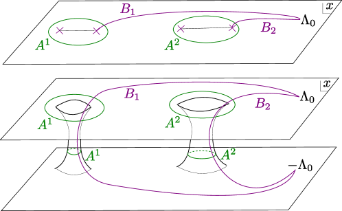
Figure 5: A Calabi-Yau three-fold with two local conifold singularities after complex deformation drawn on $x$-plane. The top figure is drawn as a double sheet cover with 2 branch-cuts, while the bottom figure is drawn as a Riemann surface. Three-cycles of Calabi-Yau 3-fold project to 1-cycles on a Riemann surface. Here drawn are compact $A^{k}$-cycles and non-compact $B_{k}$-cycles.

2 The large $N$ dual description

This section considers the large $N$ limit of such brane/anti-brane systems and find that the holographically dual closed string geometry is the identical to the supersymmetric case with just branes, except that some of the fluxes are negative. This leads, on the dual closed string side, to a metastable vacuum with spontaneously broken supersymmetry.

The supersymmetric configuration of branes for this geometry was studied in [51], which proposes a large $N$ holographic duality. The relevant Calabi-Yau geometry was obtained by a geometric transition of (1) whereby the ${S^{2}}$’s are blown down and the $n$ resulting conifold singularities at $x=e_{k}$ are resolved into $S^{3}$’s by deformations of the complex structure. See Figure 3 for a depiction of singularity resolutions of a single conifold. The new complex-deformed geometry is given by

$${\ uv=y^{2}+W^{\prime 2}+f_{n-1}(x),}$$ (5)

where $f_{n-1}(x)$ is a degree $n-1$ polynomial in $x$. As explained in [51], the geometry is effectively described by a Riemann surface which is a double cover of the $x$-plane, where the two sheets come together along $n$ cuts near $x=e_{k}$ (where the ${S^{2}}$’s used to be), as in Figure 5. The $A^{k}$ and $B_{k}$ 3-cycles of the Calabi-Yau three-fold project to 1-cycles on the Riemann surface. The geometry is characterized by the periods of the $(3,0)$ form $\Omega$,

$$S_{k}=\oint_{A^{k}}\Omega,\qquad\partial_{S_{k}}\mathcal{F}_{0}=\int_{B_{k}}\Omega.$$ (6)

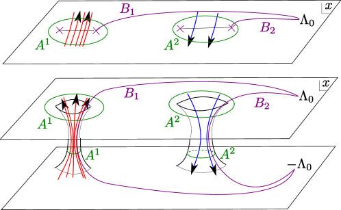
Figure 6: Amount of RR fluxes $N_{1}>0$ and $N_{2}<0$ through $A^{1}$ and $A^{2}$ 3-cycles have mixed signs.

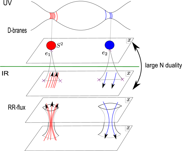
Figure 7: We have two $S^{2}$ cycles (drawn as $S^{1}$ above) in same cohomology. where we wrap brane and anti-branes. Topology allows them to move, but geometry will make it hard, because the brane tension will increase. As the number of branes $N$ increases, there will be a geometric transition, now $S^{2}$s disappear and branch cuts will open up into $S^{3}$ cycles, through which we have RR-flux. The amount of D-branes (anti-D-branes) wrapped along each $S^{2}$ is now translated into amount of RR-fluxes (negative RR-fluxes) through each $S^{3}$ cycle.

If, before the transition, all of the $S^{2}$’s were wrapped with a large number of branes, then the holographically dual type IIB string theory is given by the geometry of (5), where the branes from before the transition are replaced by fluxes

$$\oint_{A^{k}}H=N_{k},\qquad\int_{B_{k}}H=-\alpha.$$ (7)

We conjecture that this large $N$ duality holds even when $N_{k}$’s have mixed signs as in Figure 6 . The flux numbers $N_{k}$ are positive or negative depending on whether D5-branes or anti-D5-branes wrap the $k$’th $S^{2}$ before the transition, as in Figure 7. The flux through the $B_{k}$ cycles corresponds to the bare gauge coupling constant on the D-branes wrapping the corresponding ${S^{2}}$. It is independent of $k$, since the ${S^{2}}$’s are all in the same homology class. Turning on RR-fluxes generates a superpotential [52]

$$\mathcal{W}=\int H\wedge\Omega,$$ (8)

$${\mathcal{W}(S)=\sum_{k}\alpha S_{k}+N_{k}{\partial_{S_{k}}}\mathcal{F}_{0}.}$$ (9)

In the supersymmetric case studied in [51], the coefficients of the polynomial $f(x)$ determine the dual geometry and the sizes of $S_{i}$ are fixed by the requirement that

$$\partial_{S_{k}}W(S)=0,$$ (10)

giving a supersymmetric holographic dual. In the case of interest for us, with mixed fluxes, we do not expect to preserve supersymmetry. Instead we should consider the physical potential $V(S)$ and find the dual geometry by extremizing

$$\partial_{S_{k}}V(S)=0,$$ (11)

which we expect to lead to a metastable vacuum. The effective potential $V$ is given in terms of the special geometry data and the flux quanta

$$V=g^{S_{i}{\bar{S}}_{j}}\,{\partial_{S_{i}}}\mathcal{W}\,\overline{{\partial_{S_{j}}\mathcal{W}}}.$$ (12)

Here the Kähler metric is given by $g_{i{\bar{j}}}=\mathrm{Im}(\tau_{ij})$, where $\tau_{ij}$ is the period matrix of the Calabi-Yau three-fold

$$\tau_{ij}={\partial_{S_{i}}\partial_{S_{j}}}\mathcal{F}_{0}.$$ (13)

As explained in [53], the flux breaks $\mathcal{N}=2$ supersymmetry in a rather exotic way. Namely, $which$ $\mathcal{N}=1$ is preserved off-shell turns out to be a choice of a “gauge”: one can write the theory in such a way to manifest either the brane-type or the anti-brane-type of $\mathcal{N}=1$ supersymmetry. On shell, however, we have no such freedom, and only one $\mathcal{N}=1$ supersymmetry can be preserved. Which one this is depends only on whether the flux is positive or negative, and not on the choice of the $\mathcal{N}=1$ supersymmetry made manifest by the Lagrangian. The action $\mathcal{L}$ can be written in terms of $\mathcal{N}=2$ superfields, where turning on fluxes in the geometry corresponds to giving a vacuum expectation value to some of the $\mathcal{N}=2$ F-terms [54]. Since $\mathcal{N}=2$ is softly broken by the flux terms, we conjecture that the special Kähler metric is unaffected at the string tree level, but it should be modified at higher string loops.

3 The case of $2$ $S^{3}$’s

For simplicity, consider the case of just two $S^{3}$’s. Before the transition, there are two shrinking ${S^{2}}$’s at $x=e_{1},e_{2}$, as shown in Figure 4. Let $\Delta$ denote the distance between them,

$$\Delta=e_{1}-e_{2}.$$ (14)

The theory has different vacua depending on the number of branes placed on each ${S^{2}}$. The vacua with different brane/antibrane distributions are separated by energy barriers due to brane tension. To overcome these barriers, the branes must first become more massive.

The effective superpotential of the dual geometry, coming from the electric and magnetic Fayet-Iliopoulos terms turned on by the fluxes, is

$$\mathcal{W}(S)=\alpha(S_{1}+S_{2})+N_{1}{\partial_{S_{1}}}\mathcal{F}_{0}+N_{2}{\partial_{S_{2}}}\mathcal{F}_{0},$$ (15)

and the $B_{k}$-periods have been computed in terms of $A^{k}$-periods, $S_{k}$, explicitly in [51].

To leading order, dropping the quadratic terms in the $\frac{S_{k}}{g\Delta^{3}}$’s, and higher, $\tau_{ij}$ matrix elements are given by:

$${\ 2\pi i\tau_{11}} = 2\pi i\,{\partial_{S_{1}}^{2}}\mathcal{F}_{0}\approx\log(\frac{{{{S_{1}}}}}{{{{g\Delta^{3}}}}})-\log(\frac{{{{\Lambda_{0}}}}}{{\Delta}})^{2},$$ (16)

$${2\pi i\tau_{12}} = 2\pi i\,{\partial_{S_{1}}\partial_{S_{2}}}\mathcal{F}_{0}\approx-\log(\frac{{{{\Lambda_{0}}}}}{{\Delta}})^{2},$$ (17)

$${2\pi i\tau_{22}} = 2\pi i\,{\partial_{S_{2}}^{2}}\mathcal{F}_{0}\approx\log(\frac{{{{S_{2}}}}}{{{{g\Delta^{3}}}}})-\log(\frac{{{{\Lambda_{0}}}}}{{\Delta}})^{2}.$$ (18)

In particular, note that at the leading order ${\tau}_{12}$ is independent of the $S_{i}$, so we can use $\tau_{ii}$ as variables. The physical high-energy cutoff $\Lambda_{0}$ is used to compute periods of the non-compact $B_{k}$ cycles. It follows that the minima of the potential occur when

$$Re(\alpha)+Re(\tau)_{ij}N^{j} = 0,$$ (19)

$$\mathrm{Im}(\alpha)+\mathrm{Im}(\tau)_{ij}|N^{j}| = 0.$$ (20)

For example, with branes on the first ${S^{2}}$ and anti-branes on the second, one has $N_{1}>0>N_{2}$, and the metastable vacuum solution is

$${\ \left|{{S}_{1}}\right|=g\Delta^{3}\;(\frac{{{{\Lambda_{0}}}}}{{\Delta}})^{2}}\overline{{(\frac{\Lambda_{0}}{\Delta})}}{{}^{2|\frac{N_{2}}{N_{1}}|}\;e^{-2\pi i\alpha/|N_{1}|},\qquad\left|{{S}_{2}}\right|={\ g\Delta^{3}}(\frac{\Lambda_{0}}{\Delta})^{2}}\overline{{(\frac{\Lambda_{0}}{\Delta})}}{{}^{2|\frac{N_{1}}{N_{2}}|}e^{2\pi i{\ }\overline{{\alpha}}/|N_{2}|}.}$$ (21)

with its potential energy is given by

$${\ V_{\ast}^{+-}=\frac{{8\pi}}{{g_{YM}^{2}}}\,(|N_{1}|+|N_{2}|)-}\frac{{2}}{{\pi}}{{|N_{1}||N_{2}|}\;\log|\frac{\Lambda_{0}}{\Delta}|^{2}}.$$ (22)

The first term, in the holographic dual, corresponds to the tensions of the branes. The second term should correspond to the Coleman-Weinberg one loop potential, which is generated by zero point energies of the fields. This interpretation coincides nicely with the fact that this term is proportional to $|N_{1}||N_{2}|$, and thus comes entirely from the $1-2$ sector of open strings with one end on the branes and the other on the anti-branes. The fields in the $1-1$ and $2-2$ sectors (with both open string endpoints on the same type of branes) do not contribute terms proportional to $N_{i}^{2}$ to (22), as those sectors are supersymmetric and the boson and fermion contributions cancel. For comparison, in the case of where both ${S^{2}}$’s were wrapped by D5-branes, the potential at the critical point $V_{\ast}^{++}$ equals

$$V_{\ast}^{++}=\frac{{8\pi}}{{g_{YM}^{2}}}\,(|N_{1}|+|N_{2}|)=V_{\ast}^{--}$$ (23)

and is the same as for all anti-branes. This comes as no surprise, since the tensions are the same, and the interaction terms cancel since the theory is now truly supersymmetric.

We now consider the masses of bosons and fermions in the brane/anti-brane background. With supersymmetry broken, there is no reason to expect pairwise degeneracy of the four real boson masses, which come from the fluctuations of $S_{1,2}$ around the vacuum. The four bosonic masses are given by

$$\left(m_{\pm}(c)\right)^{2}=\frac{{(a^{2}+b^{2}+2abcv)\pm\sqrt{(a^{2}+b^{2}+2abcv)^{2}-4a^{2}b^{2}(1-v)^{2}}}}{{2(1-v)^{2}}}$$ (24)

where $c$ takes values $c=\pm 1$, and

$$a\equiv\left|\frac{{N_{1}}}{{2\pi\Lambda_{1}^{3}\mathrm{Im}\tau_{11}}}\right|,\qquad b\equiv\left|\frac{{N_{2}}}{{2\pi\Lambda_{2}^{3}\mathrm{Im}\tau_{22}}}\right|,\qquad v\equiv\frac{{(\mathrm{Im}\tau_{12})^{2}}}{{r\mathrm{Im}\tau_{11}\mathrm{Im}\tau_{22}}}.$$ (25)

Indeed this vacuum is metastable, because all the masses squared are strictly positive. This follows from the above formula and the fact that $v<1$ in the regime of interest $|S_{i}/g\Delta^{3}|<1$. This is a nice check on our holography conjecture, as the brane/anti-brane construction was clearly metastable. Moreover, we see that there are four real bosons, whose masses are generically non-degenerate, as expected for the spectrum with broken supersymmetry.

Since supersymmetry is completely broken from $\mathcal{N}=2$ to $\mathcal{N}=0$, we expect to find $2$ massless Weyl fermions, which are the Goldstinos. Masses of the fermions are computed and we indeed find two massless fermions. Since supersymmetry is broken these are interpreted as the Goldstinos. There are also two massive fermions, with masses

$$m_{\mathrm{f1}}=\frac{{a}}{{1-v}},\qquad m_{\mathrm{f2}}=\frac{{b}}{{1-v}}.\qquad$$ (26)

Note that $v$ controls the strength of supersymmetry breaking. In particular when $v\rightarrow 0$ the 4 boson masses become pairwise degenerate and agree with the two fermion masses $a$ and $b$, as expected for a pair of $\mathcal{N}=1$ chiral multiplets.

The mass splitting between bosons and fermions is a measure of the supersymmetry breaking. In order for supersymmetry breaking to be weak, these splittings have to be small. There are two natural ways to make supersymmetry breaking small. One way is to take the number of anti-branes to be much smaller than the number of branes, and the other way is to make the branes and anti-branes be very far from each other.

2 Breakdown of metastability

This section considers a 2-cut geometry of subsection 3, and identifies location and mode of the eventual decay by computing masses of metastable vacua. Two loop contributions to effective potential $V_{\mathrm{eff}}$  generate a preferred confining vacuum which aligns the phases of the glueball fields. In the closed string dual this preferred vacuum corresponds to a configuration where the branch cuts align along a common axis. We restrict to the case where branch cuts are along the real axis, small, and far apart.

Start with a heuristic derivation of the value of the ’t Hooft coupling for which we expect higher order corrections to $V_{\mathrm{eff}}$ to lift the metastable vacua present at weak coupling.  Recall from equation (22) that the leading order energy density of the brane/anti-brane system is:

$$E^{(0)}=\frac{8\pi}{g_{\mathrm{YM}}^{2}}\left(\left|N_{1}\right|+\left|N_{2}\right|\right)-\frac{2}{\pi}\left|N_{1}\right|\left|N_{2}\right|\log\left|\frac{\Lambda_{0}}{\Delta}\right|^{2}\mbox{\tiny.}$$ (27)

The first term corresponds to the bare tension of the branes and the second term corresponds to the Coulomb attraction between the branes.

When $\left|N_{1}\right|\gtrsim\left|N_{2}\right|$ and $N_{1}>0>N_{2}$, one has:

$$E^{(0)}\geq\frac{8\pi}{g_{\mathrm{YM}}^{2}}\left(N_{1}+N_{2}\right).$$ (28)

Loss of metastability is expected precisely when the Coulomb attraction contribution to the energy density becomes comparable to the bare tension of the branes.  This is near the regime where $E^{(0)}$ is close to saturating inequality (28).  This yields the following estimate for the breakdown of metastability:

$$\frac{1}{g_{\mathrm{YM}}^{2}\left|N_{1}\right|}\sim\log\left|\frac{\Lambda_{0}}{\Delta}\right|^{2},$$ (29)

where all factors of order unity are omitted.

This breakdown in metastability is calculable near the semi-classical expansion point, when restricted consideration to flux configurations which produce metastable vacua with the branch cuts aligned along the real axis of the complex $x$-plane.

1 Masses and the mode of instability: $N_{1}=-N_{2}$

In the case that $N_{1}=-N_{2}\equiv N$ and $\theta_{\mathrm{YM}}=0$, the lowest-energy metastable vacuum corresponds to two equal size branch cuts aligned along the real axis of the complex $x$-plane.

Here we compute the bosonic masses in order to search for the mode of instability.   We now show that the unstable mode of the system corresponds to the cuts remaining equal in size and expanding towards each other. All the other modes are stable up to this point. These facts are established by computation of the bosonic mass spectrum:

$$m_{{\mathrm{R}A}}^{2} =\frac{a^{2}}{1-v}+2a\left|N\right|\left(-\frac{10}{1+\sqrt{v}}+\frac{7}{(1-v)\pi\mathop{\mathrm{I}m}\tau_{11}}\right)$$ (30)

$$m_{{\mathrm{R}S}}^{2} =\frac{a^{2}}{1-v}+2a\left|N\right|\left(-\frac{10}{1-\sqrt{v}}+\frac{7}{(1-v)\pi\mathop{\mathrm{I}m}\tau_{11}}\right)$$ (31)

$$m_{{\mathrm{I}S}}^{2} =\frac{a^{2}}{\left(1+\sqrt{v}\right)^{2}}+2a\left|N\right|\left(\frac{10}{1+\sqrt{v}}+\frac{-3}{\left(1+\sqrt{v}\right)^{2}\pi\mathop{\mathrm{I}m}\tau_{11}}\right)$$ (32)

$$m_{{\mathrm{I}A}}^{2} =\frac{a^{2}}{\left(1-\sqrt{v}\right)^{2}}+2a\left|N\right|\left(\frac{10}{1-\sqrt{v}}+\frac{17}{\left(1-\sqrt{v}\right)^{2}\pi\mathop{\mathrm{I}m}\tau_{11}}\right).$$ (33)

Here in the above, ${\mathrm{R}A}$ denotes the real anti-symmetric mode corresponding to both $S_{i}$’s real with one cut growing while the other shrinks, ${\mathrm{R}S}$ denotes the real symmetric mode corresponding to both $S_{i}$’s real with both cuts growing in size together, and ${\mathrm{I}S}$ and ${\mathrm{I}A}$ are similarly defined for the imaginary components of the $S_{i}$’s.  Further, we have introduced the parameters:

$$a=\frac{|N|}{2\pi t\mathop{\mathrm{I}m}{\tau}_{11}}\mbox{\tiny, }v=\frac{\mathop{\mathrm{I}m}{{\tau}_{12}}^{2}}{\mathop{\mathrm{I}m}{\tau}_{11}\mathop{\mathrm{I}m}{\tau}_{22}}.$$ (34)

In equations (30-33), the term proportional to $a^{2}$ corresponds to the leading order contribution to the masses squared computed in (24), and the term proportional to $2a\left|N\right|$ corresponds to the two loop correction to this value.  As expected from symmetry, we find that as a function of $\left|N/\alpha\right|$, $m_{RS}^{2}$ approaches zero.

It is also of interest to consider the difference in masses between the bosonic and fermionic fluctuations dictated by the underlying $\mathcal{N}=2$ structure of the theory.  We find that the masses of the fermions naturally group into two sets of values.  At leading order in $1/N$, the $\mathcal{N}=2$ supersymmetry of the theory is spontaneously broken.  This indicates the presence of two massless goldstinos.  Labeling the fermionic counterparts of the gauge bosons and the $S_{i}$’s respectively by $\psi_{A}^{(i)}$ and $\psi_{S}^{(i)}$, we find that when $N_{1}=-N_{2}$, the non-zero masses of the canonically normalized fermionic fields are all equal and given by the value:

$$|m_{\psi}|=\frac{a}{\left(1-v\right)}+\left|N\right|\frac{7+10\sqrt{v}}{1-v}.$$ (35)

As before, the first term corresponds to the leading order mass and the second term is the two loop correction to this value.

We find more generally that for vacua which satisfy $S_{1}=-\overline{S_{2}}$, the system develops an instability at a similar value of $\left|N/\alpha\right|$.  In this case, the mode of instability causes the cuts to expand in size and rotate towards the real axis of the complex $x$-plane.  This is in agreement with the physical expectation that the flux lines annihilate most efficiently when the branch cuts are aligned along the real axis.

2 Breakdown of metastability: $\left|N_{1}\right|\gg\left|N_{2}\right|$

We now study the behavior of $V_{\mathrm{eff}}$ for flux configurations with $\left|N_{1}\right|\gg\left|N_{2}\right|$ and $\theta_{\mathrm{YM}}=0$, also requiring that $N_{1}$ is small enough for the two loop approximation of $V_{\mathrm{eff}}$ to be valid.  In this case, the modulus $t_{1}\equiv S_{1}/g\Delta^{3}$ fluctuates much less than $t_{2}\equiv-S_{2}/g\Delta^{3}$.

It is important to compute the masses squared of the bosonic fluctuations at the metastable minimum in order to determine the mode of instability for this flux configuration.  We find that the unstable mode corresponds to the smaller branch cut increasing in size at a much faster rate than its larger counterpart.

With the kinetic terms of the Lagrangian density canonically normalized, the $4\times 4$ bosonic mass squared matrix $m_{\mathrm{Bosonic}}^{2}$ takes the block diagonal form:

$$m_{\mathrm{Bosonic}}^{2}=A^{(R)}\oplus A^{(I)}$$ (36)

where the $A^{(R,I)}$ are $2\times 2$ matrices of the form:

$$A^{(R,I)}=\left(\begin{array}[]{cc}\frac{\left(\partial_{1}^{(R,I)}+\partial_{2}^{(R,I)}\right)^{2}V_{\mathrm{eff}}}{1+v}&-\frac{\left(\partial_{1}^{(R,I)}-\partial_{2}^{(R,I)}\right)\left(\partial_{1}^{(R,I)}+\partial_{2}^{(R,I)}\right)V_{\mathrm{eff}}}{\sqrt{1-v^{2}}}\\ -\frac{\left(\partial_{1}^{(R,I)}-\partial_{2}^{(R,I)}\right)\left(\partial_{1}^{(R,I)}+\partial_{2}^{(R,I)}\right)V_{\mathrm{eff}}}{\sqrt{1-v^{2}}}&\frac{\left(\partial_{1}^{(R,I)}-\partial_{2}^{(R,I)}\right)^{2}V_{\mathrm{eff}}}{1-v}\end{array}\right)$$ (37)

and $A^{(R)}$ (resp. $A^{(I)}$) corresponds to the mass matrix for the real (resp. imaginary) components of the $S_{i}$’s.  In the above we have defined

$$\partial_{j}^{(R)} = \frac{1}{\sqrt{\mathop{\mathrm{I}m}\tau_{jj}}}\frac{\partial}{\partial\mathop{\mathrm{R}e}S_{j}},\qquad v=\frac{\mathop{\mathrm{I}m}{{\tau}_{12}}^{2}}{\mathrm{\mathop{\mathrm{I}m}}{\tau}_{11}\mathop{\mathrm{I}m}{\tau}_{22}},$$ (38)

$$\partial_{j}^{(I)} = \frac{1}{\sqrt{\mathop{\mathrm{I}m}\tau_{jj}}}\frac{\partial}{\partial\mathop{\mathrm{I}m}S_{j}},\mbox{\tiny}$$ (39)

and for future use we also introduce:

$$a=\frac{|N_{1}|}{2\pi t_{1}\mathop{\mathrm{I}m}{\tau}_{11}}\mbox{\tiny, }\qquad b=\frac{|N_{2}|}{2\pi t_{2}\mathop{\mathrm{I}m}{\tau}_{22}}.$$ (40)

In the above expressions the components of $\tau_{ij}$ correspond to their values at the critical point of $V_{\mathrm{eff}}$ and hereafter will be treated as constants.  When $\left|N_{1}\right|>>|N_{2}|$, the masses squared and eigenmodes of the block $A^{(R)}$ are

$$m_{\mathop{\mathrm{R}e}S_{1}}^{2} =\frac{b^{2}}{(1-v)^{2}} \left(\sqrt{\frac{1-\sqrt{v}}{1+\sqrt{v}}},1\right)_{R} \oplus\left(0,0\right)_{I}$$ (41)

$$m_{\mathop{\mathrm{R}e}S_{2}}^{2} =a^{2}-2a\left(10|N_{2}|-\frac{2|N_{1}|+5|N_{2}|}{\mathop{\mathrm{I}m}{\tau}_{11}\pi}\right) \left(-\sqrt{\frac{1+\sqrt{v}}{1-\sqrt{v}}},1\right)_{R} \oplus\left(0,0\right)_{I},$$ (42)

and the masses squared and eigenmodes of the block $A^{(I)}$ are similarly given by

$$m_{\mathop{\mathrm{I}m}S_{1}}^{2} =\frac{b^{2}}{(1-v)^{2}} \left(\sqrt{\frac{1-\sqrt{v}}{1+\sqrt{v}}},1\right)_{I}\oplus \left(0,0\right)_{R}$$ (43)

$$m_{\mathop{\mathrm{I}m}S_{2}}^{2} =a^{2}+2a\left(10|N_{2}|+\frac{2|N_{1}|+5|N_{2}|}{\mathop{\mathrm{I}m}{\tau}_{11}\pi}\right) \left(-\sqrt{\frac{1+\sqrt{v}}{1-\sqrt{v}}},1\right)_{I}\oplus \left(0,0\right)_{R}\mbox{\tiny.}$$ (44)

Grouping the fermions according to the supermultiplet structure inherited from the $\mathcal{N}=1$ supersymmetry of the branes, the non-zero fermion masses are

$$m_{\psi_{S}} =\frac{1}{1-v}\left(a+\frac{2|N_{1}|+5|N_{2}|+10|N_{1}|\frac{\mathop{\mathrm{I}m}{\tau}_{12}}{\mathop{\mathrm{I}m}{\tau}_{22}}}{\mathop{\mathrm{I}m}{\tau}_{11}\pi}\right)$$ (45)

$$m_{\psi_{A}} =\frac{1}{1-v}\left(b+\frac{2|N_{2}|+5|N_{1}|+10|N_{1}|\frac{\mathop{\mathrm{I}m}{\tau}_{12}}{\mathop{\mathrm{I}m}{\tau}_{11}}}{\mathop{\mathrm{I}m}{\tau}_{22}\pi}\right),$$ (46)

with similar notation to that given above equation (35).  By inspection of the above formulae, we see that the two loop correction increases the difference between the bosonic and fermionic masses already present at leading order.

Keeping $g_{\mathrm{YM}}^{2}\left|N_{2}\right|$ fixed, we now determine the mode which develops an instability as the ’t Hooft coupling $g_{\mathrm{YM}}^{2}\left|N_{1}\right|$ approaches the critical value where the original metastable vacua disappear.  The determinant of each block of the mass matrix is:

$$\det A^{(R)} =\frac{4096\pi^{8}\log t_{1}\log t_{2}}{g_{YM}^{8}t_{1}^{2}t_{2}^{2}\left(\log t_{1}\log t_{2}-\log\frac{|{\Lambda}_{0}|^{2}}{{|\Delta|}^{2}}\left(\log t_{1}+\log t_{2}\right)\right)^{6}}$$ (47)

$$\times\left(\begin{array}[]{l}\log t_{1}\log t_{2}-20t_{1}\left(\log t_{1}\right)^{2}\left(\log\frac{|{\Lambda}_{0}|^{2}}{{|\Delta|}^{2}}-\log t_{1}\right)\\ -20t_{2}\left(\log t_{2}\right)^{2}\left(\log\frac{|{\Lambda}_{0}|^{2}}{{|\Delta|}^{2}}-\log t_{2}\right)+\cdots\end{array}\right)$$ (50)

$$\det A^{(I)} =\frac{4096\pi^{8}\log t_{1}\log t_{2}}{g_{YM}^{8}t_{1}^{2}t_{2}^{2}\left(\log t_{1}\log t_{2}-\log\frac{|{\Lambda}_{0}|^{2}}{{|\Delta|}^{2}}\left(\log t_{1}+\log t_{2}\right)\right)^{6}}$$ (51)

$$\times\left(\begin{array}[]{l}\log t_{1}\log t_{2}+20t_{1}\left(\log t_{1}\right)^{2}\left(\log\frac{|{\Lambda}_{0}|^{2}}{{|\Delta|}^{2}}-\log t_{1}\right)\\ +20t_{2}\left(\log t_{2}\right)^{2}\left(\log\frac{|{\Lambda}_{0}|^{2}}{{|\Delta|}^{2}}-\log t_{2}\right)+\cdots\end{array}\right).$$ (54)

It follows from the last line of each expression that only $m_{\mathop{\mathrm{R}e}S_{1}}^{2}$ or $m_{\mathop{\mathrm{R}e}S_{2}}^{2}$ can vanish.  Furthermore, because $m_{\mathop{\mathrm{R}e}S_{1}}^{2}>>m_{\mathop{\mathrm{R}e}S_{2}}^{2}$, the mode of instability will cause the smaller cut to expand towards the larger cut.  For $\left|N_{1}\right|\gg\left|N_{2}\right|~{}$this occurs at a value of $t_{1}$ given by:

$$1\sim 20\left(-\log t_{1}+\log\left|\frac{{\Lambda}_{0}}{{\Delta}}\right|^{2}\right)t_{1}.$$ (55)

3 Toward a global phase structure of a 2-cut metastable system

So far we have studied the case where two branch cuts are small and far apart from each other. Already this small region of moduli space exhibits a rich phase structure. It is interesting to ponder the global phase structure of this system. For example, one may ask, what happens when two cuts are near each other, or when their sizes grow? We do not yet know whether this configuration supports any supersymmetric configuration, let alone non-supersymmetric cases. In order to study the global phase structure, one needs to understand the special geometry in the whole moduli space, and compute the special geometry period there.

The organization of this section is as follows. The subsection 1 studies the structure of the moduli space, focussing on the properties of the singular points and their six-fold duality. The subsection 2 performs the integrations for the period, while restricting to the case of the real locus.

1 Study of the structure of moduli space

Consider a geometry with local deformed conifolds of (5) with $n=2$ denoting number of conifolds.

$${\ uv=y^{2}+W^{\prime 2}+f_{1}(x),}$$ (56)

with

$$W^{\prime}=g(x-e_{1})(x-e_{2}),\qquad f_{1}(x)=b_{1}x+b_{0}.$$ (57)

As explained in [51], the geometry is effectively described by a Riemann surface which is a double cover of the $x$ plane, where the two sheets come together along two branch-cuts as in Figure 5. The geometry is characterized by the periods of the $(3,0)$ form $\Omega$ over $A$ and $B$ 3-cycles as in (6). Equivalently, the period is computed from the integrating 1-form over corresponding 1-cycles of the Riemann surface as in [51],

$$dx\sqrt{W^{\prime 2}(x)+f_{1}(x)}=dx\ g\sqrt{(x-a_{1})(x-a_{2})(x-a_{3})(x-a_{4})}$$ (58)

in various segments over $x$-plane. The points at $x=a_{i}$ are the endpoints of the branch-cuts. Widths of the branch-cuts are $2\Delta_{43}$ and $2\Delta_{21}$, and $I$ denotes the distance between centers of branch-cuts. They are related by

$$\left(a_{1},a_{2},a_{3},a_{4}\right)=\left(-\Delta_{21}-\frac{I}{2},\Delta_{21}-\frac{I}{2},-\Delta_{43}+\frac{I}{2},\Delta_{43}+\frac{I}{2}\right),$$ (59)

and we have following relations

$$\frac{I^{2}}{2}-\frac{\Delta^{2}}{2}+\Delta_{21}^{2}+\Delta_{43}^{2}=0$$ (60)

$$b_{1}=I(\Delta_{21}^{2}-\Delta_{43}^{2})\sim\left(S_{1}+S_{2}\right).$$ (61)

In previous sections we used the periods computed in [51] for the small region of moduli space where $\left|\Delta_{21},\Delta_{43}\right|\ll\left|I,\Delta\right|$. These periods are written in terms of two small expansion parameters $S_{1}\sim\Delta_{21}/I$ and $S_{2}\sim\Delta_{43}/I$. To consider a global phase structure, one needs to compute the periods beyond the region of $\left|\Delta_{21},\Delta_{43}\right|\ll\left|I\right|$, so that we can obtain expressions for superpotential and effective physical potential. We would like to discover whether there still exist supersymmetric and non-supersymmetric vacua, and what kind of stability they have.

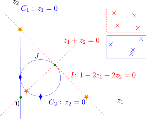
Figure 8: Moduli space and singular divisors of 2-cut geometry with $\Delta=1$. Under repairing of the endpoints of two branch cuts, some divisors will be identified with each other. Two sets of equivalent singular divisors of 2-cut geometry $\{C_{i},C_{j},J\}$ (solid) and $\{I,z_{1}=z_{2}\}$ (dashed) are drawn.            The intersection points of divisors also get identified among themselves. They are grouped into following three sets of points:

●

$(z_{1},z_{2})=(0,0),\left(\frac{1}{4},\frac{1}{4}\right)$

★

$(z_{1},z_{2})=\left(\frac{1}{8},\frac{1}{8}\right),\left(0,\frac{1}{2}\right),\left(\frac{1}{2},0\right)$

◆

$(z_{1},z_{2})=\left(0,\frac{1}{3}\right),\left(\frac{1}{3},0\right)$

Before computing the periods, let us examine the moduli space. With the variables

$$z_{1}=\frac{1}{4}\left(a_{2}-a_{1}\right)^{2}=\Delta_{21}^{2},\qquad z_{2}=\frac{1}{4}\left(a_{4}-a_{3}\right)^{2}=\Delta_{43}^{2},$$ (62)

there are four divisors (drawn in Figure 8) given by the following formulas

$$C_{1} : z_{1}=\frac{1}{4}\left(a_{2}-a_{1}\right)^{2}=0,\qquad C_{2}:z_{2}=\frac{1}{4}\left(a_{4}-a_{3}\right)^{2}=0$$ (63)

$$I : I^{2}=\Delta^{2}-2z_{1}-2z_{2}=0$$ (64)

$$J : J=(a_{1}-a_{2})(a_{2}-a_{3})(a_{3}-a_{4})(a_{1}-a_{4})=0.$$ (65)

They satisfy

$$\sum a_{i}^{2} = \Delta^{2},\qquad I(C_{1}-C_{2})=b_{1}={\mathrm{c}onstant}$$ (66)

$$\sum a_{i} = 0,\qquad C_{1}C_{2}J^{2}={\mathrm{c}onstant}.$$ (67)

The limit of $\Delta\rightarrow 0$ is another divisor $C_{\infty}$, which corresponds to branch-cuts growing much larger than the separation between cuts.

We propose following six-fold duality among intersection points of singular divisors, coming from different ways to choose two branch-cuts by pairing up four possible endpoints of branch-cuts. Divisor $I$ corresponds to the centers of cuts colliding. Additionally, one can also consider the $z_{1}=z_{2}$ locus, where two cuts are equal in size and direction (phase). The four points make a parallelogram, as in the upper box (dashed) of the Figure 8. Divisors $C_{i}$ correspond to the cuts shrinking to small sizes, bringing $a_{2i},a_{2i-1}$ together. A divisor $J$ corresponds to the branch-cuts touching each other. Two of the four endpoints will be close to each other, as in the lower box (solid) of the Figure 8. Under the permutation of $\left(a_{1},a_{2},a_{3},a_{4}\right)$ it follows easily that

$$C_{i}\leftrightarrow C_{j}\leftrightarrow J,\qquad I\leftrightarrow z_{1}=z_{2}$$ (68)

2 Computation in real locus

This section computes various integrals that are needed to obtain the periods in the real locus $\left(a_{1},a_{2},a_{3},a_{4}\right),\Lambda_{0}\in\mathbb{R}$. First consider the case where two cuts are separated by a distance; with $S_{2}$ on the right and $S_{1}$ on the left, as in Figure 9. The cut-off scale $\Lambda_{0}$ is on the far right of the endpoints of branch-cuts, $\Lambda_{0}\gg a>b>c>d$, which are ordered as

$$\left(d,c,b,a\right)=\left(-\Delta_{21}-\frac{I}{2},\Delta_{21}-\frac{I}{2},-\Delta_{43}+\frac{I}{2},\Delta_{43}+\frac{I}{2}\right).$$ (69)

Without loss of generality one may assume that the first cut is smaller than the second cut: $\Delta_{21}\leq\Delta_{43}$.

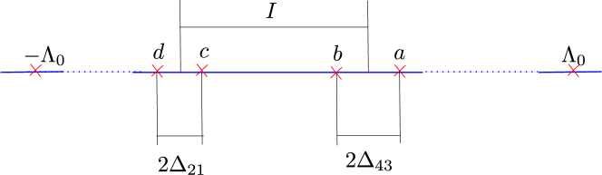
Figure 9: Two branch cuts are aligned along the real axis and separated.

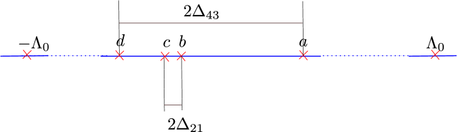
Figure 10: One small branch cut is living inside a larger branch cut.

Now compute integrals over compact cycles and then over a non-compact cycle between the cutoff $\Lambda_{0}$ and $S_{2}$ as in (58)

$$I_{R} \equiv \int_{b}^{a}dx\sqrt{|(x-a)(x-b)(x-c)(x-d)|}$$ (70)

$$I_{L} \equiv \int_{d}^{c}dx\sqrt{|(x-a)(x-b)(x-c)(x-d)|}$$ (71)

$$I_{M} \equiv \int_{c}^{b}dx\sqrt{|(x-a)(x-b)(x-c)(x-d)|}$$ (72)

$$I_{NR} \equiv \int_{a}^{\Lambda_{0}}dx\sqrt{|(x-a)(x-b)(x-c)(x-d)|}.$$ (73)

The integrals over compact cycles in the real locus is expressed in closed form in terms of elliptic integrals as in [55]. The non-compact cycle is Taylor-expanded below in terms of a small variable.

The integrals $I_{L},I_{R},I_{M},I_{NR}$ are given below to 4th order in $\Delta_{21}$ by

$$I_{R} = \frac{\pi}{2\sqrt{1+2s^{2}}}\left(\Delta_{43}^{2}+(-1+c-s^{2})\Delta_{21}^{2}+\frac{\left(1+2s^{2}\right)(-1-7c^{2}+4c^{3}+4c^{5})}{8c^{3}}\Delta_{21}^{4}\right),$$

$$I_{L} = \frac{\pi}{2\sqrt{1+2s^{2}}}\left(c\Delta_{21}^{2}+\frac{\left(1+2s^{2}\right)\left(-1-7c^{2}\right)}{8c^{3}}\Delta_{21}^{4}\right),$$

$$I_{NR} = \frac{\Lambda_{0}^{3}}{3}-\frac{\Lambda_{0}}{4}+\frac{1-6s^{2}\log\left[\frac{2\Lambda_{0}}{\Delta_{43}}\right]}{12\left(1+2s^{2}\right)^{\frac{3}{2}}}+\frac{-2c^{2}\tanh^{-1}c+(1+s^{2})\log\left[\frac{2\Lambda_{0}}{\Delta_{43}}\right]}{\ 2\sqrt{1+2s^{2}}}\Delta_{21}^{2}$$

$$+ \frac{\sqrt{1+2s^{2}}}{16c^{4}}\left(2c\left(-1-7c^{2}\right)\tanh^{-1}c-4c^{2}\left(2-s^{2}\right)\log\left[\frac{2\Lambda_{0}}{\Delta_{43}}\right]+\left(5-6s^{2}\right)\right)\Delta_{21}^{4},$$

$$I_{M} = \frac{1}{12\left(1+2s^{2}\right)^{\frac{3}{2}}}\left(\begin{array}[]{c}2c(1+s^{2})+3s^{3}(\pi-2\theta)\\ +6cs^{2}\log\left[\frac{\Delta_{21}}{4c^{2}}s\sqrt{1+2s^{2}}\right]\end{array}\right)$$ (76)

$$+ \frac{\Delta_{21}^{2}}{8c^{3}\sqrt{1+2s^{2}}}\left(\begin{array}[]{c}-2+9s^{2}-13s^{4}+5s^{6}\\ +c^{3}s(-2+s^{2})(\pi-2\theta)\\ +(-4+s^{2}+2s^{4})s^{2}\log\left[\frac{\Delta_{21}}{4c^{2}}s\sqrt{1+2s^{2}}\right]\end{array}\right)$$ (80)

$$+ \frac{\sqrt{1+2s^{2}}\Delta_{21}^{4}}{256c^{7}}\left(\begin{array}[]{c}-48+304s^{2}-1422s^{4}+2121s^{6}-1286s^{8}+284s^{10}\\ +8c^{7}s(-4+11s^{2})(\pi-2\theta)\\ +2s^{2}(8-252s^{2}+481s^{4}-340s^{6}+88s^{8})\log\left[\frac{\Delta_{21}}{4c^{2}}s\sqrt{1+2s^{2}}\right]\end{array}\right),$$ (84)

where we denote $(c,s)=(\cos\theta,\sin\theta)$ where $\theta$ is given by

$$\Delta_{43}=\frac{\sin\theta}{\sqrt{2\sin^{2}\theta+1}}.$$ (85)

Now consider the case where a small cut $S_{1}$ is inside a larger cut $S_{2}$ as in Figure 10. The endpoints of branch-cuts are ordered as

$$\left(a_{1},a_{2},a_{3},a_{4}\right)=\left(d,c,b,a\right)=\left(-\Delta_{43}+\frac{I}{2},-\Delta_{21}-\frac{I}{2},\Delta_{21}-\frac{I}{2},\Delta_{43}+\frac{I}{2}\right).$$ (86)

The integrals $I_{R},I_{L},I_{M},I_{NR}$ are given to 4th order to $\Delta_{21}$ by

$$I_{R} = \frac{I}{4cs}\left(\begin{array}[]{c}\left(\frac{c}{6}+\frac{s(\pi+2\theta^{\prime})}{4(2+s^{2})}\right)+\frac{\Delta_{21}^{2}}{4}\left(c(-1+2\log\left[\frac{\Delta_{21}s}{4c^{2}I}\right])-2s(\pi+2\theta^{\prime})\right)\\ +\frac{\Delta_{21}^{4}(2+s^{2})}{64c^{3}}\left(17-28s^{2}+8s^{4}+4(-5+4s^{2})\log\left[\frac{\Delta_{21}s}{4c^{2}I}\right]\right)\end{array}\right),$$ (89)

$$I_{L} = \frac{I}{4s}\left(\begin{array}[]{c}\left(\frac{c}{6}-\frac{s(\pi-2\theta^{\prime})}{4(2+s^{2})}\right)+\frac{\Delta_{21}^{2}}{4}\left(c(-1+2\log\left[\frac{\Delta_{21}s}{4c^{2}I}\right])+2s(\pi-2\theta^{\prime})\right)\\ +\frac{\Delta_{21}^{4}(2+s^{2})}{64c^{3}}\left(17-28s^{2}+8s^{4}+4(-5+4s^{2})\log\left[\frac{\Delta_{21}s}{4c^{2}I}\right]\right)\end{array}\right),$$ (92)

$$I_{M} = \frac{c\pi}{4}\left(\Delta_{21}\frac{1-s}{2+s^{2}}+\frac{\Delta_{21}^{2}I}{s}+\frac{\Delta_{21}^{3}\ }{8c^{4}}\left(9+4s-8s^{2}-4s^{3}\right)+\frac{\Delta_{21}^{4}s}{8c^{4}I}\left(-5+4s^{2}\right)\right),$$

$$I_{NR} = \frac{\Lambda_{0}^{3}}{3}-\frac{\Lambda_{0}}{4}+\frac{I^{3}}{12s^{2}}\left(s^{2}-6\log\left[\frac{2\Lambda_{0}s}{I}\right]\right)+\frac{\Delta_{21}^{2}I}{4s}\left(4s\log\left[\frac{2\Lambda_{0}s}{I}\right]+c\left(\pi-2\theta^{\prime}\right)\right)$$

$$- \frac{\Delta_{21}^{4}s}{32c^{3}I}\left(2sc\left(-3+2s^{2}\right)+(5-4s^{2}\right)(\pi-2\theta^{\prime}))$$

again $(c,s)=(\cos\theta^{\prime},\sin\theta^{\prime})$ where $\theta^{\prime}$ is given by

$$I=\frac{\sin\theta^{\prime}}{\sqrt{2+\sin^{2}\theta^{\prime}}}.$$ (93)

Chapter 3 Stable vacua with D5-branes and a varying Neveu-Schwarz flux

This chapter considers $\mathcal{N}=1$ supersymmetric theories with a field-dependent gauge coupling. A novel mechanism for spontaneous supersymmetry breaking is observed to result from negative squared gauge couplings, and we obtain meta- and it exactly stable vacua.

The set-up is following: Consider the case of D5-branes wrapped on vanishing cycles in local Calabi-Yau 3-folds, and then turn on a Neveu-Schwarz background $B$-field $\alpha(x)$ which depends holomorphically on one complex coordinate $x$ of the 3-fold. Using large $N$ duality via a geometric transition as in the previous chapter, we show how the strongly coupled IR dynamics can be understood using string theoretic techniques.

If the background field $\alpha(x)$ is chosen appropriately, there are vacua exhibiting broken supersymmetry. A suitable choice of higher-dimensional operators can lead to negative values of $g_{\mathrm{YM}}^{2}$ for certain factors of the gauge group, which leads to supersymmetry breaking. In the string theory framework, this arises from the presence of anti-branes in a holomorphic $B$-field background.

The organization of the rest of the chapter is as follows. Section 1 provides the string theory construction in terms of $N$ D5-branes. The closed string dual at large $N$ is presented in section 2. Section 3 studies supersymmetry breaking mechanisms.

1 The string theory construction

Consider type IIB string theory compactified on the Calabi-Yau 3-fold defined by

$${uv=y^{2}-W^{\prime 2},}$$ (1)

with the superpotential $W$

$$W(x)=\sum_{k=1}^{n+1}a_{k}x^{k},\qquad W^{\prime}(x)=g\prod_{i=1}^{n}(x-e_{i}).$$ (2)

At each of $n$ critical points $x=e_{i}$ of $W$, the geometry develops a conifold singularity, which is resolved by a minimal ${S^{2}}$. (See Figures 3 and 4.) We choose $N_{i}$ of the D5-branes to wrap the $i$’th ${S^{2}}$. This is similar to the considerations of the section 2, except that we allow a varying holomorphic Neveu-Schwarz field. In particular, the tree-level gauge coupling for the branes wrapping the ${S^{2}}$ at $x=e_{i}$ is given by

$${\int_{{S^{2}}_{i}}B_{0}=\left(\frac{\theta}{2\pi}+\frac{4\pi i}{g_{\mathrm{YM}}^{2}}\right)_{i}=\alpha(e_{i}).}$$ (3)

2 The closed string dual

The open-string theory on D5-branes at UV has a dual description in terms of pure geometry with fluxes at IR. In flowing to the IR, the D5-branes deform the geometry around them so that the ${S^{2}}$’s they wrap vanish, while the $S^{3}$’s surrounding the branes obtain finite sizes, as depicted in Figure (3) for a single conifold. After the geometric transition, the geometry is complex-deformed from that given by (1) to the manifold

$${uv=y^{2}-W^{\prime 2}+f_{n-1}(x)}.$$ (4)

Here $f_{n-1}(x)$ is a polynomial in $x$ of degree $n-1$, the $n$ coefficients of which govern the sizes of the $n$ resulting $S^{3}$’s.

The effective superpotential is classical in the dual geometry and is generated by fluxes

$$\mathcal{W}_{\mathrm{eff}}=\int_{CY}H\wedge\Omega,$$ (5)

where $\Omega$ is a holomorphic three-form on the Calabi-Yau three-fold

$$\Omega=\frac{{dx\wedge dy\wedge dz}}{z}.$$ (6)

The effective superpotential is computed in [56]

$${{\mathcal{W}}_{\mathrm{eff}}=\sum_{k=1}^{n}N_{k}}\frac{{\partial}}{{{\partial S_{k}}}}{{\ \mathcal{F}}_{0}+\oint_{A_{k}}\alpha(x)ydx.}$$ (7)

3 Supersymmetry breaking

This section studies the phase structure of the $\mathcal{N}=1$ models introduced in the section 1. We find that there is a region in the parameter space where supersymmetry is broken. This leads to novel and calculable mechanisms for breaking supersymmetry.

The organization of the rest of the section is as follows. Subsection 1 studies the situation of all $\mathrm{Im}\,\alpha(e_{i})$ negative. Subsection 2 turns on NS-field which varies holomorphically, and the internal dynamics of the gauge theory softly breaks supersymmetry. Subsection 3 considers metastable supersymmetry breaking mechanism of the multi-sign case, and subsection 4 studies its decay.

1 Negative gauge couplings and flop of $S^{2}$

Consider $N$ D5-branes on the resolved conifold geometry with a single ${S^{2}}$, and turn on a $constant$ $B$-field through the ${S^{2}}$,

$$\alpha=\frac{{\theta}}{{2\pi}}+\frac{{4\pi i}}{{g_{\mathrm{YM}}^{2}}}=\int_{S_{x}^{2}}\bigl{(}B_{\mathrm{RR}}+\frac{{i}}{{g_{s}}}{\ B_{\mathrm{NS}}}\bigr{)}.$$

By changing the $B$-field, an $S^{2}$ undergoes a flop, into a new ${S^{2}}$ with negative area. Moreover, the charge of the wrapped D5-branes on this flopped ${S^{2}}$ is opposite to what it was before the flop. Therefore, in order to conserve D5-brane charge across the flop, anti-D5-branes appear on the new ${S^{2}}$ instead of D5-branes.

In the case of constant $B$-field, we again obtain a $U(N)$ gauge theory with $\mathcal{N}=1$ supersymmetry at low energies. However, the $\mathcal{N}=1$ supersymmetry that the theory preserves after the flop has to be orthogonal to the original one, since branes and antibranes preserve different supersymmetries.

Figure 1: Start by wrapping $N_{1},N_{2}>0$ branes on $S^{2}$’s located at resolved singular points $x=e^{1},e^{2}$. As we flop the second $S^{2}$, the second stack of branes will turn into a stack of anti-branes, in order to hold the same Gauss’s law holds true for RR-charge.

2 Supersymmetry breaking by background Neveu-Schwarz fluxes

Now consider the same geometry as in the previous subsection, but with a holomorphically varying NS $B$-field introduced. Wrapping branes on the conifold gives rise to supersymmetric theories. However, in the case of anti-branes, supersymmetry is in fact broken. This arises from the fact that, while branes preserve the same half of the background ${\mathcal{N}=2}$ supersymmetry as the $B$-field, anti-branes preserve an opposite half.

As in the previous section, this section considers branes and anti-branes on the conifold geometry, but now with the holomorphically varying $B$-field given by:

$${\ B(x)=t_{0}+t_{2}x^{2}.}$$ (8)

This can be studied from the perspective of the IR effective field theory of the glueball superfield $S$. Because of the underlying ${\mathcal{N}=2}$ structure of this theory, we will have a valid IR description regardless of whether it is branes or anti-branes which are present.

Recall from (7) that the superpotential in the dual geometry is

$${{\mathcal{W}}(S)=-\oint_{A}B(x)ydx+N{\frac{\partial{\mathcal{F}}_{0}}{\partial S}}.}$$ (9)

The first term may be explicitly calculated as:

$$\oint_{A}B(x)ydx=t_{0}S+t_{2}\frac{{S^{2}}}{m}.$$

The scalar potential is again given by (12) with the same metric and prepotential $\mathcal{F}_{0}$, but now with superpotential (9). The vacua which extremize the potential $\partial_{S}V_{\mathrm{eff}}=0$ satisfy one of following:

$$-\left(t_{0}+2t_{2}\frac{{S}}{m}\right)+N\tau = 0,$$ (10)

$$-\left(t_{0}+2t_{2}\frac{{S}}{m}\right)+N{\bar{\tau}}+4\pi i(\tau-\bar{\tau})t_{2}\frac{{S}}{m} = 0.$$ (11)

The solution to (10) also satisfies $\partial\mathcal{W}=0$, and corresponds to the case where branes are present, with

$$\mathrm{Im}[\alpha]\gg 0,$$

where

$$\alpha=t_{0}+2t_{2}\frac{S}{m}.$$ (12)

Large positive values of $\mathrm{Im}[\alpha]$ give $|S/m|\ll|\Lambda_{0}^{2}|$ within the allowed region. This vacuum is manifestly supersymmetric.

Instead, study anti-branes by allowing the geometry to undergo a flop, so that

$$\mathrm{Im}[\alpha]\ll 0.$$ (13)

Then the supersymmetric solution is unphysical, and we instead study solutions to (11). One can directly observe the fact that supersymmetry is broken in this vacuum by computing the tree-level masses of the bosons and fermions in the theory, and showing that there is a nonzero mass splitting.

The fermion masses may be read off from the $\mathcal{N}=1$ Lagrangian as

$${\Lambda^{-4}m_{\psi}} {=} \frac{{1}}{{{2i\left(\mathrm{Im}\tau\right)^{2}}}}\frac{{1}}{{2\pi iS}}{\left(t_{0}+N\bar{\tau}+2t_{2}\frac{{S}}{m}\right)+\ }\frac{{1}}{{{\mathrm{Im}\tau}}}\frac{{{2t_{2}}}}{m}$$

$${\Lambda^{-4}m_{\lambda}} {=} \frac{{1}}{{{2i\left(\mathrm{Im}\tau\right)^{2}}}}\frac{{1}}{{2\pi iS}}{\overline{\left(t_{0}+N\tau+2t_{2}\frac{{S}}{m}\right)}},$$

while the bosonic masses are computed to be

$$\Lambda^{-4}m_{b,\pm}^{2}=\frac{{1}}{{\mathrm{Im}\tau}}\left(\partial\bar{\partial}{V_{\mathrm{eff}}}\pm\left|\partial\partial{V_{\mathrm{eff}}}\right|\right).$$

By evaluation of the masses in the brane vacuum, it follows that $\lambda$ is a massless fermion which acts as a partner of the massless gauge field $A$, while $\psi$ is a superpartner to $S$. In other words, supersymmetry pairs up the bosons with fermions of equal mass.

Evaluating the masses in the anti-brane vacuum, $\psi$ becomes the massless goldstino. However, there is no longer a bose/fermi degeneracy like where the background $B$-field was constant. Instead,

$${m_{b,\pm}^{2}=|m_{\lambda}|^{2}\pm 4\pi\Lambda^{4}|m_{\lambda}\partial\alpha|.}$$ (14)

This mass splitting shows quite explicitly that all supersymmetries are broken in this vacuum. Since this supersymmetry breaking can occur within a conifold, we call this domestic supersymmetry breaking.

3 Multi-cut geometry and supersymmetry breaking

Previously we have focused on the case where all gauge couplings have the same sign, positive or negative. More generally, expand consideration to the more general case in which both signs are present. This gives inter-conifold supersymmetry breaking, involving D-brane stacks on multiple conifolds. The mass splittings of bosons and fermions are explicitly computed in [56]. Interestingly, the vacuum energy density formula is now given by:

$$\frac{{{{V_{\mathrm{eff}}}_{\ast}}}}{{{\Lambda^{4}}}}{={2\sum_{i}N_{i}{\left(|\mathrm{Im}\,\alpha_{i}|-\mathrm{Im}\,\alpha_{i}\right)}}+\left(\sum_{i,j}^{\delta_{i}>0,\delta_{j}<0}{\frac{2}{\pi}}N_{i}N_{j}\log\left|{\frac{\Lambda_{0}}{\Delta_{ij}}}\right|\right).}$$ (15)

Here, the first term is the brane tension contribution from each flopped ${S^{2}}$ with negative $g_{\mathrm{YM}}^{2}$ and the second term suggests that opposite brane types interact to contribute a repulsive Coulomb potential energy,as in the cases considered in [58].

4 Decay mechanism for non-supersymmetric systems

It is straightforward to see how the non-supersymmetric systems studied in this section can decay. This is particularly clear in the UV picture. If the gauge coupling constants are all negative, the branes want to sit at the critical point $x=e_{i}$ with the smallest $|\mathrm{Im}B(e_{i})|$, minimizing vacuum energy according to (15). Thus we expect that in this case the system will decay to the $U(N)$ theory of antibranes in a holomorphic $B$-field background. Although this breaks supersymmetry, it is completely stable. Considering that RR charge has to be conserved, no further decay is possible.

If there are some critical points at which $\mathrm{Im}B(e_{i})$ is positive, there is no unique stable vacuum. Instead, there are precisely as many vacua as number of ways distribute $N$ branes amongst the critical points $x=e_{i}$ where $\mathrm{Im}B(e_{i})>0$. Any of these numerous supersymmetric vacua could be the end point of the decay process.

Chapter 4 A Dirac neutrino model in an F-theory $SU(5)$ Grand Unified Theory Model

The discovery of neutrino oscillations [59, 60] has revealed that neutrinos have small but non-zero mass. However, massive neutrinos cannot be explained in the Standard Model of particle physics without introducing extra ingredients. As such, neutrino physics offers a concrete and exciting window into physics beyond the Standard Model.

Aspects of flavor physics in F-theory Grand Unified Theories have been studied in [61], where it was shown that with the minimal number of geometric ingredients necessary for achieving one heavy generation, the resulting flavor hierarchies in the quark and charged lepton sectors are in accord with observation. The aim of this chapter is to extend this minimal framework to include a neutrino sector with viable flavor physics using the supersymmetry breaking and mediation mechanisms of [62].

We present a Dirac neutrino model in a minimal $SU(5)$ F-theory GUT, which leads to a phenomenologically consistent model of neutrino flavor. (This work was previously published in [63], which also studies a Majorana neutrino scenario.) Integrating out massive Kaluza-Klein modes generates higher dimension operators which generate viable neutrino masses. The neutrino mass scale $m_{\nu}$ is roughly related to the weak scale $M_{\mbox{\tiny weak}}$ and a scale close to $M_{\mathrm{G}UT}$ through the numerology of the seesaw mechanism:

$$m_{\nu}\sim\frac{M_{\mbox{\tiny weak}}^{2}}{\Lambda_{\mbox{\tiny UV}}}.$$ (1)

In the Dirac scenario, the D-term

$$\lambda_{ij}^{\mbox{\tiny Dirac}}\int\mathrm{d}^{4}\theta\frac{H_{d}^{{\dagger}}L^{i}N_{R}^{j}}{\Lambda_{\mbox{\tiny UV}}}$$ (2)

is generated by integrating out massive modes on the Higgs down curve. Supersymmetry breaking leads to an F-term for $H_{d}^{{\dagger}}$ of order ${F_{H_{d}}}\sim\mu H_{u}\sim M_{\mbox{\tiny weak}}^{2}$, inducing a Dirac mass.

The supersymmetry breaking sector of [62] naturally enters the discussion of neutrino physics. In [62], the absence of a bare $\mu$ term in the low energy theory was ascribed to the presence of a $U(1)$ Peccei-Quinn symmetry, derived from an underlying $E_{6}$ GUT structure.

Estimating the form of the Yukawa matrices for the operator (2), we find that in both scenarios the neutrinos exhibit a “normal” hierarchy, where the two lightest neutrinos are close in mass. The participation of Kaluza-Klein modes dilutes the mass hierarchy in comparison to the quark and charged lepton sectors. More precisely, the resulting neutrino mass hierarchy is roughly:

$$m_{1}:m_{2}:m_{3}\sim\alpha_{\mathrm{G}UT}:\alpha^{1/2}_{\mathrm{G}UT}:1$$ (3)

which is in reasonable accord with the observed neutrino mass splittings.

The structure of the neutrino mixing matrix displays a mild hierarchical structure. The two mixing angles $\theta_{12}$ and $\theta_{23}$ are found to be comparable, and in rough agreement with experiments. The mixing angle $\theta_{13}$, which measures mixing between the heaviest and lightest neutrino (in our normal hierarchy), is predicted to be roughly given (in radians) by:

$$\theta_{13}\sim\theta_{C}\sim\alpha_{\mathrm{G}UT}^{1/2}\sim 0.2\mbox{\tiny,}$$ (4)

where $\theta_{C}$ denotes the Cabibbo angle.

The organization of the rest of the chapter is as follows. Section 1 provides a short review of those aspects of F-theory GUTs which are of relevance to neutrino physics. A Dirac neutrino model is presented in section 2. Our results for the neutrino masses and mixing angles are compared with experiments in section 3.

1 Minimal F-theory Grand Unified Theories

In this section we briefly review the main features of minimal F-theory GUTs, focusing on those aspects of particular relevance to neutrino physics. For further background and review, see [64]. We also discuss in greater detail the role of the anomalous global $U(1)$ Peccei-Quinn symmetry in the supersymmetry breaking sector of the low energy theory, and its interplay with the neutrino sector.

F-theory is defined as a strongly coupled formulation of IIB string theory in which the profile of the axio-dilaton $\tau_{IIB}$ is allowed to vary over the ten-dimensional spacetime (see Figure 1.).

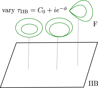
Figure 1: F-theory is a non-perturbative extension of type IIB string theory with coupling constant $\tau_{\mathrm{I}IB}$ allowed to vary over a complex number with $SL(2,Z)$ symmetry of a 2-torus

In F-theory GUTs, the gauge degrees of freedom of the GUT group propagate in the bulk of the seven-brane wrapping a complex surface $S$. The type of singular fibers over $S$ decides the GUT group, which in the present, minimal case corresponds to $SU(5)$. The chiral matter and Higgs fields of the MSSM localize on 2d Riemann surfaces (complex curves) in $S$. The Yukawa couplings of the model localize near points where at least three such matter curves intersect.

Breaking the GUT group requires introducing a non-trivial flux in the $U(1)_{Y}$ hypercharge direction of the GUT group [65, 66]. The resulting unbroken gauge group in four dimensions is then given by $SU(3)_{C}\times SU(2)_{L}\times U(1)_{Y}$. Doublet-triplet splitting in the Higgs sector can be achieved by requiring that this flux pierces the Higgs up and Higgs down curves.

Generating an appropriate value for the $\mu$ term in F-theory GUTs requires a specific scale of supersymmetry breaking $\sqrt{F}\sim 10^{8}-10^{9}$ GeV. F-theory GUTs appear to more naturally accommodate minimal gauge-mediated supersymmetry breaking scenarios.

We shall focus our attention on vacua with a minimal number of additional geometric and field theoretic ingredients required to obtain phenomenologically viable low energy physics.

1 $U(1)_{\mathrm{P}Q}$ and neutrinos

Selection rules in string based constructions sometimes forbid interaction terms in the low energy theory. In the specific context of F-theory GUTs, the $U(1)_{\mathrm{P}Q}$ symmetry plays an especially prominent role in that it forbids a bare $\mu$ and $B\mu$ term in the low energy theory. Indeed, $U(1)_{\mathrm{P}Q}$ symmetry breaking and supersymmetry breaking are tightly correlated in the deformation away from gauge mediation [62].

In order to explain why $\mu$ can be far smaller than the GUT scale, we forbid the bare $\mu$-term

$$\mu H_{u}H_{d}\mbox{\tiny,}$$ (5)

by imposing a global $U(1)_{\mathrm{P}Q}$ symmetry under which the Higgs up and Higgs down have $U(1)_{\mathrm{P}Q}$ charges $q_{H_{u}}$ and $q_{H_{d}}$ with $q_{H_{u}}+q_{H_{d}}\neq 0$.

In the context of F-theory GUTs, correlating the value of the $\mu$ term with supersymmetry breaking is achieved using the higher dimensional operator:

$$L_{\mathrm{e}ffective}\supset\int\mathrm{d}^{4}\theta\frac{X^{{\dagger}}H_{u}H_{d}}{\Lambda_{\mbox{\tiny UV}}}\mbox{\tiny.}$$ (6)

Here, $X$ is a chiral superfield localized on a matter curve normal to the GUT seven-brane. The curves $X$, $H_{u}$ and $H_{d}$ have a triple intersection and the operator (6) results from integrating out Kaluza-Klein modes on the curve on which $X$ localizes. This necessarily requires that $X$ be charged under $U(1)_{\mathrm{P}Q}$ with charge:

$$q_{X}=q_{H_{u}}+q_{H_{d}}\mbox{\tiny.}$$ (7)

When $X$ develops a supersymmetry breaking vev:

$$\left\langle X\right\rangle=x+\theta^{2}F_{X}\mbox{\tiny,}$$ (8)

inducing an effective $\mu$ term of order:

$$\mu\sim\frac{\overline{F_{X}}}{\Lambda_{\mbox{\tiny UV}}}\mbox{\tiny.}$$ (9)

Using the fact that $\Lambda_{\mbox{\tiny UV}}\mathrel{\mathstrut\smash{\ooalign{\raise 2.5pt\hbox{$<$}\cr\lower 2.5pt\hbox{$\sim$}}}}M_{\mathrm{G}UT}$, generating a value for the $\mu$ term near the scale of electroweak symmetry breaking requires $\sqrt{F_{X}}\sim 10^{8}-10^{9}$ GeV [62].

As explained in [62], this type of structure is compatible with an underlying $E_{6}$ symmetry. The $U(1)_{\mathrm{P}Q}$ charges of the various fields are:

$$X$$

(10)

where $Y$ and $Y^{\prime}$ denote the messenger fields of the gauge mediation sector. In addition to forbidding a bare $\mu$ term, a $\mathbb{Z}_{2}$ subgroup of $U(1)_{\mathrm{P}Q}$ can naturally be identified with matter parity of the MSSM. Indeed, by inspection of the above charges, note that the charges of the MSSM chiral matter are all odd, while the Higgs fields are even.

2 A Dirac scenario

In this section we study minimal F-theory GUT scenarios which incorporate Dirac masses through higher dimension operators of the effective theory. The right-handed neutrinos correspond to four-dimensional zero modes of the compactification. Kaluza-Klein mode excitations of the higher dimensional theory play a prominent role in setting the overall mass scale of the neutrino sector. When the Higgs down, lepton doublet and right-handed neutrino curves intersect at a point, the required D-term is generated by integrating out massive modes localized on the Higgs down curve.

A suggestive link between the neutrino, weak and GUT scales is present in Dirac scenarios where the Dirac mass term is generated by the higher dimension operator

$$\int\mathrm{d}^{4}\theta\frac{H_{d}^{{\dagger}}LN_{R}}{\Lambda_{\mbox{\tiny UV}}}.$$ (11)

This operator is generated in an analogous fashion to the Giudice-Masiero operator $X^{{\dagger}}H_{u}H_{d}/\Lambda_{\mbox{\tiny UV}}$ obtained in [62] where $\Lambda_{\mbox{\tiny UV}}$ is close to $M_{\mathrm{G}UT}$. Moreover the resulting scale of the neutrino mass is automatically right: Indeed, the most important feature of the usual GUT scale seesaw is that:

$$m_{\nu}\sim\frac{M_{\mbox{\tiny weak}}^{2}}{\Lambda_{\mbox{\tiny UV}}}\sim\frac{v_{u}^{2}}{\Lambda_{\mbox{\tiny UV}}}\sim\frac{\overline{F_{H_{d}}}}{\Lambda_{\mbox{\tiny UV}}},$$ (12)

where as usual, $v_{u}$ denotes the scale of the Higgs up vev, and $F_{H_{d}}$ denotes the F-term component of the $H_{d}$ superfield. Note that $F_{H_{d}}$ converts the D-term to a Dirac mass term for the neutrinos:

$$\int\mathrm{d}^{4}\theta\frac{H_{d}^{{\dagger}}LN_{R}}{\Lambda_{\mbox{\tiny UV}}}\rightarrow\int\mathrm{d}^{2}\theta\frac{\mu\langle H_{u}\rangle LN_{R}}{\Lambda_{\mbox{\tiny UV}}}.$$ (13)

This last equality follows from the fact that the MSSM superpotential contains the $\mu$-term

$$W_{MSSM}\supset\mu H_{u}H_{d},$$ (14)

so that the F-term equation of motion yields:

$$\overline{F_{H_{d}}}\sim\frac{\partial W_{MSSM}}{\partial H_{d}}\sim\mu\left\langle H_{u}\right\rangle\sim 10^{5}\mbox{GeV}^{2}\mbox{\tiny}.$$ (15)

Here we have used the fact that the $\mu$ parameter is typically between $500-1000$ GeV in F-theory GUTs[62].

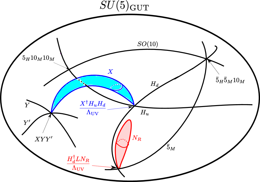
Figure 2: Matter fields and Yukawa interaction terms in an F-theory $SU(5)$ Grand Unified Theory model with Dirac neutrinos. Right-handed neutrino $N_{R}$ and messenger $X$ do not transform under $SU(5)$. Corresponding matter curves for these $SU(5)$ singlets do not live on the $SU(5)$ GUT brane and stick out of the page.

1 Generating higher dimensional operators

We now demonstrate that the higher dimension operator:

$$L\supset\frac{\lambda_{ij}^{\mbox{\tiny Dirac}}}{\Lambda_{\mbox{\tiny UV}}}\int\mathrm{d}^{4}\theta H_{d}^{{\dagger}}L^{i}N_{R}^{j}$$ (16)

is generated by integrating out massive modes localized on the Higgs down curve. Here the right-handed neutrinos localize on a curve which is normal to the GUT seven-brane. See Figure 2 for a depiction of a minimal F-theory GUT which contains a Dirac neutrino sector. This operator can originate from a point of triple-intersection of the Higgs down, lepton doublet and right-handed neutrino curves.

The higher-dimensional action is expressed in terms of an infinite collection of $\mathcal{N}=1$ four-dimensional chiral superfields, each labeled by points of the internal directions of the compactification. The operator of (16) is obtained by integrating out massive modes localized on the Higgs down curve. Labeling the higher-dimensional fields by points of the threefold base, the relevant interaction terms are given by:

$$L\supset\int_{B_{3}}\mathrm{d}^{4}\theta\mathcal{H}_{d}^{{\dagger}}\mathcal{H}_{d}+\int_{B_{3}}\mathrm{d}^{2}\theta\mathcal{H}_{d}^{c}\mathcal{LN}+\int_{B_{3}}\mathrm{d}^{2}\theta\mathcal{H}_{d}^{c}\overline{\partial}_{\mathcal{A}}\mathcal{H}_{d}\mbox{\tiny.}$$ (17)

The F-term equation of motion for $\mathcal{H}_{d}^{c}$ yields

$$\overline{\partial}_{\mathcal{A}}\mathcal{H}_{d}+\mathcal{LN}=0\mbox{\tiny,}$$ (18)

so that

$$\mathcal{H}_{d}=H_{d}-\frac{1}{\overline{\partial}_{\mathcal{A}}^{\prime}}\mathcal{LN}\mbox{\tiny,}$$ (19)

where $H_{d}$ denotes the four-dimensional massless mode solution. Plugging $\mathcal{H}_{d}$ back into the effective action of (17), one obtains the effective operator

$$\frac{\lambda_{ij}^{\mbox{\tiny Dirac}}}{\Lambda_{\mbox{\tiny UV}}}\int\mathrm{d}^{4}\theta H_{d}^{{\dagger}}L^{i}N_{R}^{j}=\int_{B_{3}}\mathrm{d}^{4}\theta H_{d}^{{\dagger}}\frac{1}{\overline{\partial}_{\mathcal{A}}^{\prime}}L^{i}N_{R}^{j}\mbox{\tiny.}$$ (20)

In other words, the relevant Yukawa matrix is given by the overlap integral

$$\frac{\lambda_{ij}^{\mbox{\tiny Dirac}}}{\Lambda_{\mbox{\tiny UV}}}=\int_{B_{3}}\overline{\Psi}_{H_{d}}\frac{1}{\overline{\partial}_{\mathcal{A}}^{\prime}}\Psi_{L}^{i}\Psi_{N}^{j}\mbox{\tiny,}$$ (21)

where the $\Psi$’s denote the zero mode wave functions. This can be rewritten in bra-ket notation by inserting a complete basis of states, so that the Dirac Yukawa reduces to a sum over massive states $\left|\Psi_{\mathcal{H}}\right\rangle$

$$\frac{\lambda_{ij}^{\mbox{\tiny Dirac}}}{\Lambda_{\mbox{\tiny UV}}}=\underset{\Psi_{\mathcal{H}}}{\sum}\left\langle\Psi_{H_{d}}|\Psi_{\mathcal{H}}\right\rangle\frac{1}{M_{\Psi_{\mathcal{H}}}}\left\langle\Psi_{\mathcal{H}}|\Psi_{L}^{i}\Psi_{N}^{j}\right\rangle\mbox{\tiny.}$$ (22)

It follows that to estimate the structure of $\lambda_{ij}^{\mbox{\tiny Dirac}}/\Lambda_{\mbox{\tiny UV}}$, it is enough to compute the overlap of the massive mode wave functions localized on the Higgs down curve with the lepton doublet and neutrino zero mode wave functions

$$\left\langle\Psi_{\mathcal{H}}|\Psi_{L}^{i}\Psi_{N}^{j}\right\rangle=\int_{\mathcal{U}_{B}}\overline{\Psi}_{\mathcal{H}}\Psi_{L}^{i}\Psi_{N}^{j}\mbox{\tiny.}$$ (23)

Here in the above, $\mathcal{U}_{B}$ denotes a patch in $B_{3}$ containing the neutrino interaction point.

2 Neutrino Yukawa matrix

The zero mode wave functions $\Psi_{L}^{i}$ and $\Psi_{N}^{j}$ can be organized according to order in $z_{L,N}$ so that

$$\Psi_{L}^{i}\sim\left(\frac{z_{L}}{R_{L}}\right)^{3-i}\mbox{\tiny, }\qquad\Psi_{N}^{j}\sim\left(\frac{z_{N}}{R_{N}}\right)^{3-j}\mbox{\tiny}.$$ (24)

Here $z_{L}$ (resp. $z_{N}$) denotes a local coordinate for the lepton doublet (resp. neutrino) curve, and $R_{L}$ (resp. $R_{N}$) denotes the characteristic length scale of this curve. The crucial point is that the massive modes will overlap with the zero mode wave functions, inducing maximal violation of the corresponding $U(1)$ coordinate rephasing symmetries in the directions transverse to the Higgs down curve. Indeed, the massive mode wave function $\Psi_{\mathcal{H}}^{I_{L},I_{N}}$ will contain contributions of the form

$$\Psi_{\mathcal{H}}^{I_{L},I_{N}}\supset\left(\frac{\overline{z_{L}}}{R_{\ast}}\right)^{i}\left(\frac{\overline{z_{N}}}{R_{\ast}}\right)^{j}\exp\left(-\frac{z_{L}\overline{z_{L}}}{R_{\ast}^{2}}-\frac{z_{N}\overline{z_{N}}}{R_{\ast}^{2}}\right)$$ (25)

for all $i\leq I_{L}$, $j\leq I_{N}$. It now follows that the overlap is given by

$$\langle\Psi_{\mathcal{H}}^{I_{L},I_{N}}|\Psi_{L}^{i}\Psi_{N}^{j}\rangle\sim\sqrt{\varepsilon_{L}^{3-i}\varepsilon_{N}^{3-j}}\theta_{3-i}(I_{L})\theta_{3-j}(I_{N})\mbox{\tiny}.$$ (26)

Here $\theta_{3-i}(I)$ denotes a step function which is $1$ for $I\geq 3-i$, and $0$ for $I<3-i$, and we have introduced the small parameters

$$\varepsilon_{L}\equiv\left(\frac{R_{\ast}}{R_{L}}\right)^{2}\mbox{\tiny, }\qquad\varepsilon_{N}\equiv\left(\frac{R_{\ast}}{R_{N}}\right)^{2}\mbox{\tiny.}$$ (27)

Summing over all of the massive mode contributions in equation (22), it now follows that the Dirac matrix is given by

$$\frac{\lambda_{(\nu)}^{\mbox{\tiny Dirac}}}{\Lambda_{\mbox{\tiny UV}}}\sim\frac{\Sigma}{M_{\ast}}\begin{pmatrix}\varepsilon_{L}\varepsilon_{N}&\varepsilon_{L}^{1/2}\varepsilon_{N}&\varepsilon_{N}\\ \varepsilon_{L}\varepsilon_{N}^{1/2}&\varepsilon_{L}^{1/2}\varepsilon_{N}^{1/2}&\varepsilon_{N}^{1/2}\\ \varepsilon_{L}&\varepsilon_{L}^{1/2}&1\end{pmatrix}\sim\frac{\Sigma}{M_{\ast}}\begin{pmatrix}\varepsilon^{2}&\varepsilon^{3/2}&\varepsilon\\ \varepsilon^{3/2}&\varepsilon&\varepsilon^{1/2}\\ \varepsilon&\varepsilon^{1/2}&1\end{pmatrix}\mbox{\tiny,}$$ (28)

where $\Sigma$ denotes the contribution from the convolution of the wave functions by the Green’s function, and where the final relation uses the approximation $\varepsilon_{L}\sim\varepsilon_{N}\sim\varepsilon\sim\sqrt{\alpha_{\mathrm{G}UT}}$.

3 Comparison with experiments

Let us first examine the PMNS neutrino mixing matrix [67, 68] :

$$U_{\mathrm{PMNS}}=U_{L}^{(l)}\left(U_{L}^{(\nu)}\right)^{{\dagger}}=\left(\begin{array}[]{ccc}c_{12}c_{13}&s_{12}c_{13}&s_{13}e^{-i\delta}\\ -s_{12}c_{23}-c_{12}s_{23}s_{13}e^{i\delta}&c_{12}c_{23}-s_{12}s_{23}s_{13}e^{i\delta}&s_{23}c_{13}\\ s_{12}s_{23}-c_{12}c_{23}s_{13}e^{i\delta}&-c_{12}s_{23}-s_{12}c_{23}s_{13}e^{i\delta}&c_{23}c_{13}\end{array}\right)\cdot D_{\alpha}$$

where $D_{\alpha}=$ diag$(e^{i\alpha_{1}/2},e^{i\alpha_{2}/2},1)$, $c_{ij}=\cos\theta_{ij}$ and $s_{ij}=\sin\theta_{ij}$. $\delta$, $\alpha_{1}$ and $\alpha_{2}$ are CP violating phases.

By diagonalizing the Yukawa interaction matrix of (28), we get

$$U_{\mathrm{PMNS}}^{\mathrm{F-th}}\sim\left(\begin{array}[]{ccc}U_{e1}&\varepsilon^{1/2}&\varepsilon\\ \varepsilon^{1/2}&U_{\mu 2}&\varepsilon^{1/2}\\ \varepsilon&\varepsilon^{1/2}&U_{\tau 3}\end{array}\right)$$ (29)

with $\varepsilon\sim\sqrt{\alpha_{\mathrm{G}UT}}\sim 0.2$ for the Dirac scenario of the previous section. Ignoring CP violating phases, each entry has following magnitude

$$\left|U_{\mathrm{PMNS}}^{\mathrm{F-th}}\right|\sim\begin{pmatrix}0.87&0.45&0.2\\ 0.45&0.77&0.45\\ 0.2&0.45&0.87\end{pmatrix},$$ (30)

in remarkable agreement with experimental results in [69, 70].

$$\left|U_{\mathrm{PMNS}}^{3\sigma}\right|\sim\left(\begin{array}[]{ccc}0.77-0.86&0.50-0.63&0.00-0.22\\ 0.22-0.56&0.44-0.73&0.57-0.80\\ 0.21-0.55&0.40-0.71&0.59-0.82\end{array}\right),$$ (31)

displaying a remarkable agreement. Note that we predict a rather large value of upper right corner, $\sin\theta_{13}\sim 0.2$, and we are delighted that there is new experimental result confirming the largeness of $\theta_{13}$ angle [71].

Next, consider the ratio of neutrino mass eigenvalues. Our model predicts mild “normal hierarchy” $m_{1}:m_{2}:m_{3}\sim\varepsilon^{2}:\varepsilon:1$ with $\varepsilon\sim\sqrt{\alpha_{\mathrm{G}UT}}\sim 0.2$. If one assumes normal hierarchy, the experimental data automatically gives $m_{3}^{\mathrm{observe}}\sim\sqrt{\Delta m_{31}^{2}}\sim 50\pm 4\ {\mathrm{m}eV}$, $m_{2}^{\mathrm{observe}}\sim\sqrt{\Delta m_{21}^{2}}\sim 8.7\pm 0.4\ {\mathrm{m}eV}$, and our F-theory model predicts the smallest mass eigenvalue to be $m_{1}^{\mathrm{F-th}}\sim 1-3\ {\mathrm{m}eV}.$

The Dirac neutrino scenario prohibits double beta decay, but the alternative Majorana scenario in [63] predicts the double beta decay mass $\left|m_{\beta\beta}\right|^{2}=\left|\underset{i=1}{\overset{3}{\sum}}m_{i}\left(U_{ei}^{\mathrm{PMNS}}\right)^{2}\right|^{2}$ to be $m_{\beta\beta}^{\max}\sim 6\ {\mathrm{m}eV}$. This may be observed within ten years. The EXO experiment is expected to be sensitive down to 4-40 meV [72]. For single beta decay $\left|m_{\beta}\right|^{2}=\underset{i=1}{\overset{3}{\sum}}m_{i}^{2}\left|U_{ei}^{\mathrm{PMNS}}\right|^{2}$, we predict $\left|m_{\beta}^{\mathrm{F-th}}\right|\sim 5-10\ {\mathrm{m}eV}$, which is too small to be observed soon. The KATRIN experiment is expected to be sensitive down to 0.2 eV [73].

Chapter 5 Conclusion and open problems

We discussed the importance and relevance of string theory in the realm of theoretical physics. If one wants to connect string theory to the real world, the first job is to get rid of extra dimensions and to break supersymmetry while maintaining stability of the vacuum. This thesis discussed various supersymmetry breaking mechanisms in heterotic and type IIB string theories, and generation of neutrino mass scale due to supersymmetry breaking in an F-theory $SU(5)$ Grand Unified Theory model.

We considered BPS and non-BPS states in heterotic string theory compactified on $T^{4}$. A non-BPS state can decay into a set of BPS states with the same total charge and smaller total mass. We organized conservation of the charges using a set of eight $16\times 16$ transformation matrices and constrained possible decay modes allowed by charge conservation. We constructed a non-BPS state which is rather robust against decays into BPS states. We identified its huge stability region in moduli space of $T^{4}$, proving that no other decays into BPS states are possible. We constructed a non-BPS state which does not require fine tuning of moduli for its stability, and it will be interesting to use this in a string-inspired model building. The study of non-BPS objects and their stability may also provide non-trivial tests of weak-strong duality between heterotic string theory compactified on $T^{4}$ and type IIA string theory on an orbifold limit of a K3 surface.

With the similar objective of breaking supersymmetry without sacrificing stability, we proposed various mechanisms for metastable and exactly stable vacua in type IIB string theory. These goals were achieved by wrapping D-branes and anti-D-branes on cycles in a non-compact Calabi-Yau three-fold. A geometric transition was employed to take the large $N$ holographic dual to a flux-only picture with no branes in a new geometry, corresponding to a low energy effective theory in IR. We further investigated its phase structure and loss of classical stability.

In order to determine the global phase structure, it remains to compute explicit expressions for the periods in regions of moduli space other than in the locus where the branch cuts are small and far apart. We studied the properties of the moduli space and performed various integrals in the real locus. It would be interesting to extend these results by determining whether large $N$ duality still holds in other regions of moduli space. It remains an open problem to determine whether the (non-) supersymmetric solutions exist and whether they are stable.

We also considered meta- and exactly stable non-supersymmetric systems of type IIB string theory by turning on a Neveu-Schwarz field. Variation of this field can drive the gauge coupling squared into negative, which corresponds to a flop of the complexified Kähler class.

Our metastable vacua in the type IIB string theory setup has dual descriptions in type IIA string theory and M-theory, expressed in terms of D4-branes and anti-D4-branes hanging between 2 NS5-branes [74, 75], and in terms of M5-branes, respectively. It would be interesting to determine the brane configuration of the exactly stable supersymmetry-breaking vacua in type IIA string theory and M-theory.

Finally, we showed that an F-theory Grand Unified Theory model yields neutrino masses with mass ratios $m_{1}:m_{2}:m_{3}\sim\alpha_{\mathrm{G}UT}:\alpha_{\mathrm{G}UT}^{1/2}:1$ and a mixing matrix with large $\theta_{13}$. The supersymmetry breaking mechanism provided in [62] solves Higgs mass term $\mu$ problem and provides the correct neutrino mass scale.

We plan to continue our investigations by building string phenomenology models using the above meta- and exactly stable supersymmetry breaking configurations as a hidden sector. Also, we would like to determine whether our results carry over to a compact geometry, in order to have realistic gravity in 4D. F-theory local GUT models still need to pass the global consistency test. It is therefore crucial to understand what constraints global geometry imposes on F-theory model-building and the phenomenological implications of the decoupling limit.

References

- [1] R. Gilmore, Alice in Quantumland: An Allegory of Quantum Physics. Springer, 1995.
- [2] M. Kaku, Hyperspace: A Scientific Odyssey through Parallel Universes, Time Warps, and the Tenth Dimension. Oxford University Press, 1994.
- [3] B. Greene, The Elegant Universe: Superstrings, Hidden Dimensions, and the Quest for the Ultimate Theory. W. W. Norton Company, 2003.
- [4] G. Kane, Supersymmetry: Unveiling the Ultimate Laws of Nature. Basic Books, 2001.
- [5] L. Randall, Warped Passages: Unraveling the Mysteries of the Universe’s Hidden Dimensions. Harper Perennial, 2006.
- [6] J. Polchinski, String Theory I II. Cambridge University Press, 1998.
- [7] M. B. Green, J. H. Schwarz, and E. Witten, Superstring Theory. Cambridge University Press, 1988.
- [8] K. Becker, M. Becker, and J. H. Schwarz, String Theory and M-Theory: A Modern Introduction. Cambridge University Press, 2007.
- [9] M. Kaku, Strings, Conformal Fields, and M-Theory. Springer, 2000.
- [10] J. Wess and J. Bagger, Supersymmetry and Supergravity. Princeton University Press, 1992.
- [11] M. Nakahara, Geometry, Topology and Physics. Taylor Francis, 2003.
- [12] C. Vafa, “Lectures on strings and dualities,” hep-th/9702201.
- [13] B. R. Greene, “String theory on Calabi-Yau manifolds,” hep-th/9702155.
- [14] P. S. Aspinwall, “K3 surfaces and string duality,” hep-th/9611137.
- [15] J. D. Lykken, “Introduction to supersymmetry,” hep-th/9612114.
- [16] A. Neitzke and C. Vafa, “Topological strings and their physical applications,” hep-th/0410178.
- [17] S. Nam, String Cosmos. Chiho Publishing House, 2007.
- [18] A. Jackson, “Inteview with Heisuke Hironaka,” Notices of the American Mathematical Society 52 (8, 2005).
- [19] J. Polchinski and E. Witten, “Evidence for Heterotic - Type I String Duality,” Nucl. Phys. B460 (1996) 525–540, hep-th/9510169.
- [20] E. Witten, “String theory dynamics in various dimensions,” Nucl. Phys. B443 (1995) 85–126, hep-th/9503124.
- [21] P. H. Ginsparg, “Comment on Toroidal Compactification of Heterotic Superstrings,” Phys. Rev. D35 (1987) 648.
- [22] M. Dine, Supersymmetry and String Theory: Beyond the Standard Model. Cambridge University Press, 2007.
- [23] R. N. Mohapatra, Unification and Supersymmetry. Springer, 2002.
- [24] R. N. Mohapatra and P. B. Pal, Massive Neutrinos in Physics and Astrophysics. World Scientific Publishing Company, 2004.
- [25] M. A. Luty, “2004 TASI lectures on supersymmetry breaking,” hep-th/0509029.
- [26] S. Ferrara, L. Girardello, and F. Palumbo, “A General Mass Formula in Broken Supersymmetry,” Phys. Rev. D20 (1979) 403.
- [27] E. Witten, “Dynamical Breaking of Supersymmetry,” Nucl. Phys. B188 (1981) 513.
- [28] G. F. Giudice and A. Masiero, “A Natural Solution to the mu Problem in Supergravity Theories,” Phys. Lett. B206 (1988) 480–484.
- [29] A. Sen, “Non-BPS states and branes in string theory,” hep-th/9904207.
- [30] S. Mukhi and N. V. Suryanarayana, “A stable non-BPS configuration from intersecting branes and antibranes,” JHEP 06 (2000) 001, hep-th/0003219.
- [31] A. Sen, “Stable non-BPS states in string theory,” JHEP 06 (1998) 007, hep-th/9803194.
- [32] A. Sen, “Type I D-particle and its interactions,” JHEP 10 (1998) 021, hep-th/9809111.
- [33] E. Witten, “D-branes and K-theory,” JHEP 12 (1998) 019, hep-th/9810188.
- [34] A. Sen, “SO(32) spinors of type I and other solitons on brane- antibrane pair,” JHEP 09 (1998) 023, hep-th/9808141.
- [35] A. Sen, “Tachyon condensation on the brane antibrane system,” JHEP 08 (1998) 012, hep-th/9805170.
- [36] M. R. Gaberdiel and A. Sen, “Non-supersymmetric D-brane configurations with Bose-Fermi degenerate open string spectrum,” JHEP 11 (1999) 008, hep-th/9908060.
- [37] A. Sen, “BPS D-branes on non-supersymmetric cycles,” JHEP 12 (1998) 021, hep-th/9812031.
- [38] B. Stefanski, Jr., “Dirichlet branes on a Calabi-Yau three-fold orbifold,” Nucl. Phys. B589 (2000) 292–314, hep-th/0005153.
- [39] S. Mukhi, N. V. Suryanarayana, and D. Tong, “Brane-antibrane constructions,” JHEP 03 (2000) 015, hep-th/0001066.
- [40] J. H. Schwarz, “TASI lectures on non-BPS D-brane systems,” hep-th/9908144.
- [41] M. R. Gaberdiel, “Lectures on non-BPS Dirichlet branes,” Class. Quant. Grav. 17 (2000) 3483–3520, hep-th/0005029.
- [42] O. Bergman and M. R. Gaberdiel, “Non-BPS states in heterotic-type IIA duality,” JHEP 03 (1999) 013, hep-th/9901014.
- [43] K. S. Narain, M. H. Sarmadi, and E. Witten, “A Note on Toroidal Compactification of Heterotic String Theory,” Nucl. Phys. B279 (1987) 369.
- [44] K. S. Narain, “New Heterotic String Theories in Uncompactified Dimensions 10,” Phys. Lett. B169 (1986) 41.
- [45] D. J. Gross, J. A. Harvey, E. J. Martinec, and R. Rohm, “Heterotic String Theory. 1. The Free Heterotic String,” Nucl. Phys. B256 (1985) 253.
- [46] J. Maiden, G. Shiu, and B. Stefanski, Jr., “D-brane spectrum and K-theory constraints of , orientifolds,” JHEP 04 (2006) 052, hep-th/0602038.
- [47] N. Quiroz and B. Stefanski, Jr., “Dirichlet branes on orientifolds,” Phys. Rev. D66 (2002) 026002, hep-th/0110041.
- [48] J. Majumder and A. Sen, “Non-BPS D-branes on a Calabi-Yau orbifold,” JHEP 09 (2000) 047, hep-th/0007158.
- [49] K. A. Intriligator, N. Seiberg, and D. Shih, “Dynamical SUSY breaking in meta-stable vacua,” JHEP 04 (2006) 021, hep-th/0602239.
- [50] C. Vafa, “Superstrings and Topological Strings at Large ,” J. Math. Phys. 42 (2001) 2798–2817, hep-th/0008142.
- [51] F. Cachazo, K. Intriligator, and C. Vafa, “A Large Duality via a Geometric Transition,” Nucl. Phys. B 603 (2001) 3–41, hep-th/0103067.
- [52] S. Gukov, C. Vafa, and E. Witten, “CFT’s From Calabi-Yau Four-folds,” Nucl. Phys. B 584 (2000) 69–108 [Erratum–ibid. B 608 (2001) 477–478], hep-th/9906070.
- [53] M. Aganagic, C. Beem, J. Seo, and C. Vafa, “Geometrically induced metastability and holography,” Nucl. Phys. B789 (2008) 382–412, hep-th/0610249.
- [54] I. Antoniadis, H. Partouche, and T. R. Taylor, “Spontaneous Breaking of Global Supersymmetry,” Phys. Lett. B372 (1996) 83–87, hep-th/9512006.
- [55] M.-x. Huang and A. Klemm, “Holomorphic anomaly in gauge theories and matrix models,” JHEP 09 (2007) 054, hep-th/0605195.
- [56] M. Aganagic, C. Beem, J. Seo, and C. Vafa, “Extended Supersymmetric Moduli Space and a SUSY/Non-SUSY Duality,” Nucl. Phys. B822 (2009) 135–171, 0804.2489.
- [57] M. Atiyah, J. M. Maldacena, and C. Vafa, “An M-theory flop as a large duality,” J. Math. Phys. 42 (2001) 3209–3220, hep-th/0011256.
- [58] M. Aganagic, C. Beem, and B. Freivogel, “Geometric Metastability, Quivers and Holography,” Nucl. Phys. B795 (2008) 291–333, 0708.0596.
- [59] B. T. Cleveland et. al., “Measurement of the solar electron neutrino flux with the Homestake chlorine detector,” Astrophys. J. 496 (1998) 505–526.
- [60] Super-Kamiokande Collaboration, Y. Fukuda et. al., “Evidence for oscillation of atmospheric neutrinos,” Phys. Rev. Lett. 81 (1998) 1562–1567, hep-ex/9807003.
- [61] J. J. Heckman and C. Vafa, “Flavor Hierarchy From F-theory,” arXiv:0811.2417 [hep-th].
- [62] J. J. Heckman and C. Vafa, “F-theory, GUTs, and the Weak Scale,” arXiv:0809.1098 [hep-th].
- [63] V. Bouchard, J. J. Heckman, J. Seo, and C. Vafa, “F-theory and Neutrinos: Kaluza-Klein Dilution of Flavor Hierarchy,” JHEP 01 (2010) 061, 0904.1419.
- [64] J. J. Heckman, “Particle Physics Implications of F-theory,” 1001.0577.
- [65] C. Beasley, J. J. Heckman, and C. Vafa, “GUTs and Exceptional Branes in F-theory - II: Experimental Predictions,” JHEP 01 (2009) 059, arXiv:0806.0102 [hep-th].
- [66] R. Donagi and M. Wijnholt, “Breaking GUT Groups in F-Theory,” arXiv:0808.2223 [hep-th].
- [67] B. Pontecorvo, “Mesonium and antimesonium,” Sov. Phys. JETP 6 (1957) 429.
- [68] Z. Maki, M. Nakagawa, and S. Sakata, “Remarks on the unified model of elementary particles,” Prog. Theor. Phys. 28 (1962) 870.
- [69] M. C. Gonzalez-Garcia and M. Maltoni, “Phenomenology with Massive Neutrinos,” Phys. Rept. 460 (2008) 1–129, 0704.1800.
- [70] M. C. Gonzalez-Garcia, “Neutrino Physics,” arXiv:0901.2505 [hep-ph].
- [71] MINOS Collaboration, J. M. Paley, “Recent Results and Future Prospects from MINOS,” arXiv:0901.2131 [hep-ex].
- [72] EXO Collaboration, K. O’Sullivan, “The Enriched Xenon Observatory,” J. Phys. Conf. Ser. 120 (2008) 052056.
- [73] KATRIN Collaboration, A. Osipowicz et. al., “KATRIN: A next generation tritium beta decay experiment with sub-eV sensitivity for the electron neutrino mass,” hep-ex/0109033.
- [74] K. Ohta and T.-S. Tai, “Extended MQCD and SUSY/non-SUSY duality,” JHEP 09 (2008) 033, 0806.2705.
- [75] J. Marsano, K. Papadodimas, and M. Shigemori, “Nonsupersymmetric Brane/Antibrane Configurations in Type IIA and M Theory,” Nucl. Phys. B789 (2008) 294–361, 0705.0983.