Abstract

Kakimizu complex of a knot is a flag simplicial complex whose vertices correspond to minimal genus Seifert surfaces and edges to disjoint pairs of such surfaces. We discuss a general setting in which one can define a similar complex. We prove that this complex is contractible, which was conjectured by Kakimizu. More generally, the fixed-point set (in the Kakimizu complex) for any subgroup of an appropriate mapping class group is contractible or empty. Moreover, we prove that this fixed-point set is non-empty for finite subgroups, which implies the existence of symmetric Seifert surfaces.

1 Introduction

We study a generalisation $MS(E)$ of the following simplicial complex $MS(L)$ defined by Kakimizu [K]. Let $E=E(L)$ be the exterior of a tubular neighbourhood of a knot $L$ in ${\mathbb{S}}^{3}$. A spanning surface is a surface properly embedded in $E$, which is contained in some Seifert surface for $L$. Let $\mathcal{MS}(L)$ be the set of isotopy classes of spanning surfaces which have minimal genus. The vertex set of $MS(L)$ is defined to be $\mathcal{MS}(L)$. Vertices $\sigma,\sigma^{\prime}\in\mathcal{MS}(L)$ span an edge if they have representative spanning surfaces which are disjoint. Simplices are spanned on all complete subgraphs of the $1$–skeleton. In other words, $MS(L)$ is the flag complex spanned on its $1$–skeleton. Kakimizu defines $MS(L)$ for links in the same way, but we later argue that this is not the right definition and we define our $MS(E)$ for $E=E(L)$ differently. However, for all links whose $MS(L)$ have been so far studied we have $MS(E(L))=MS(L)$.

The general setting in which we define $MS(E(L))$, or more generally $MS(E,\gamma,\alpha)$, is the following. Let $E$ be a compact connected orientable, irreducible and $\partial$–irreducible $3$–manifold. In particular, for any non-splittable link $L$ in ${\mathbb{S}}^{3}$, the complement $E(L)$ of a regular neighbourhood of $L$ satisfies these conditions. Let $\gamma$ be a union of oriented disjoint simple closed curves on $\partial E$, which does not separate any component of $\partial E$. For $E=E(L)$ an example of $\gamma$ is the set of longitudes of all link components (or its subset). We fix a class $\alpha$ in the homology group $H_{2}(E,\partial E,{\mathbb{Z}})$ satisfying $\partial\alpha=[\gamma]$. For $E=E(L)$ and $\gamma$ the set of longitudes, there is only one choice for $\alpha$. It is the homology class dual to the element of $H^{1}(E,{\mathbb{Z}})$ mapping all oriented meridian classes onto a fixed generator of ${\mathbb{Z}}$. A spanning surface is an oriented surface properly embedded in $E$ in the homology class $\alpha$ whose boundary is homotopic with $\gamma$.

We now define the simplicial complex $MS(E,\gamma,\alpha)$, which we abbreviate to $MS(E)$, if $E=E(L)$ and $\gamma$ is the set of all longitudes. The vertex set of $MS(E,\gamma,\alpha)$ is defined to be $\mathcal{MS}(E,\gamma,\alpha)$, the set of isotopy classes of spanning surfaces which have minimal genus. However, we span an edge on $\sigma,\sigma^{\prime}\in\mathcal{MS}(E,\gamma,\alpha)$ only if they have representatives $S\in\sigma,S^{\prime}\in\sigma^{\prime}$ such that the (connected) lift of $E\setminus S^{\prime}$ to the infinite cyclic cover associated with $\alpha$ intersects exactly two lifts of $E\setminus S$. In the terminology of Section 2 this means that the Kakimizu distance between $\sigma$ and $\sigma^{\prime}$ equals one. This is not always true for disjoint $S,S^{\prime}$ (because they are allowed to be disconnected). This error is made by Kakimizu [K, formula 1.3(b)] who does not distinguish between $MS(L)$ and $MS(E(L))$. However, both his and our article prove that the right complex to consider is $MS(E(L))$.

For every link $L$ it is a basic question to determine the complex $MS(E(L))$ which encodes the structure of the set of all minimal genus spanning surfaces. This has been done for all prime knots of at most 10 crossings by Kakimizu [K2, Theorem A]. Moreover, questions about common properties of all $MS(E(L))$ (or rather $MS(L)$) have been asked. Here is a brief summary (for a broader account, see [Pe]).

Scharlemann–Thompson proved [ST, Proposition 5] that $MS(E(L))$ is connected, in the case where $L$ is a knot. Later Kakimizu [K, Theorem A] provided another proof for links. Schultens [S, Theorem 6] proved that, in the case where $L$ is a knot, $MS(E(L))$ is simply-connected (see also [SS] for atoroidal genus $1$ knots). For atoroidal knots bounds on the diameter of $MS(E(L))$ have been obtained ([Pe, SS]). Kakimizu conjectured (see [Sa, Conjecture 0.2]) that $MS(L)$ is contractible. This was verified for special arborescent links by Sakuma [Sa, Theorem 3.3 and Proposition 3.11], and announced for special prime alternating links by Hirasawa–Sakuma [HS]. In the present article, we confirm this conjecture, under no hypothesis, for the complex $MS(E,\gamma,\alpha)$.

Theorem 1.1.

$MS(E,\gamma,\alpha)$ is contractible.

Using the same method we are also able to establish the following. Note that for $E=E(L)$ all mapping classes of $E$ fix $\alpha$ and the homotopy class of $\gamma$.

Theorem 1.2.

Let $G$ be a finite subgroup of the mapping class group of $E$ fixing $\alpha$ and the homotopy class of $\gamma$. We consider its natural action on $MS(E,\gamma,\alpha)$. Then there is a simplex in $MS(E,\gamma,\alpha)$ fixed by all elements of $G$.

Sakuma argued [Sa, Proposition 4.9(1)] (see also [S, Theorem 5] for knots) that the set of vertices of any simplex of $MS(E,\gamma,\alpha)$ can be realised as a union of pairwise disjoint spanning surfaces. Hence in the language of spanning surfaces Theorem 1.2 amounts to the following.

Corollary 1.3.

Let $G$ be a finite subgroup of the mapping class group of $E$ fixing $\alpha$ and the homotopy class of $\gamma$. Then there is a union of pairwise disjoint spanning surfaces of minimal genus which is $G$–invariant up to isotopy.

In the case where $E$ is atoroidal and $\partial E$ is a union of tori, its interior admits, by the work of Thurston and the theorem of Prasad, a unique complete hyperbolic structure. Then the mapping class group of $E$ coincides with the isometry group of its interior, hence it is finite. Moreover, after deforming the metric in a way discussed in [Pe, Chapter 10] we can assume that each element of $\mathcal{MS}(E,\gamma,\alpha)$ has a unique representative of minimal area. In this case Corollary 1.3 gives the following.

Corollary 1.4.

If $E$ is atoroidal and $\partial E$ is a union of tori, then there is a union of pairwise disjoint spanning surfaces of minimal genus which is invariant under any isometry fixing $\alpha$ (the homotopy class of $\gamma$ is then fixed automatically). In particular, if $E=E(L)$, then this union is invariant under any isometry.

A related result concerning periodic knots was proved in Edmonds [E].

Finally, Theorem 1.1 turns out to be a special case ($G$ trivial) of the following.

Theorem 1.5.

Let $G$ be any subgroup of the mapping class group of $E$ fixing $\alpha$ and the homotopy class of $\gamma$. Then its fixed-point set $\mathrm{Fix}_{G}(MS(E,\gamma,\alpha))$ is either empty or contractible.

We decided to provide first the proof of Theorem 1.1 and then the more technically involved proof of the generalisation, Theorem 1.5.

We conclude with the following consequence of Theorem 1.5.

Corollary 1.6.

Denote by $G$ the mapping class group of $E$ fixing $\alpha$ and the homotopy class of $\gamma$. Let $\mathcal{F}$ be the set of those subgroups of $G$ which stabilise a point in $MS(E,\gamma,\alpha)$. Then $MS(E,\gamma,\alpha)$ is the model for $E_{\mathcal{F}}(G)$ (the classifying space for $G$ with respect to the family $\mathcal{F}$, see [L]).

Actually, it is not clear to us what groups, apart from all finite ones (see Theorem 1.2), belong to the family $\mathcal{F}$. It is also not clear if $MS(E,\gamma,\alpha)$ can be locally infinite.

Outline of the idea. We now outline the main idea of the article. The central object is the projection map $\pi$, which assigns to a pair of vertices $\sigma,\rho\in\mathcal{MS}(E,\gamma,\alpha)$ at distance $d>0$ a vertex $\pi_{\sigma}(\rho)$ adjacent to $\rho$ at distance $d-1$ from $\sigma$. Kakimizu [K] used the projection to prove that $MS(E(L))$ is connected, but in fact he did not need to verify that it is well-defined — he worked only with representatives of vertices. We verify that $\pi$ is well-defined using a result of Oertel on cut-and-paste operations on surfaces with simplified intersection.

We explain how to prove contractibility of $MS(E,\gamma,\alpha)$. Assume for simplicity that $MS(E,\gamma,\alpha)$ is finite (which is the case for $E$ hyperbolic, see [Th, Corollary 8.8.6(b)]). We fix some $\sigma\in\mathcal{MS}(E,\gamma,\alpha)$. Then we prove that among vertices farthest from $\sigma$ there exists a vertex $\rho$ which is strongly dominated by $\pi_{\sigma}(\rho)$. This means that all the vertices adjacent to $\rho$ are also adjacent to or equal $\pi_{\sigma}(\rho)$. Hence there is a homotopy retraction of $MS(E,\gamma,\alpha)$ onto the subcomplex spanned by all the vertices except $\rho$. Proceeding in this way we retract the whole complex onto $\sigma$.

Remaining questions. Finally, we indicate that questions about the structure of the set of all incompressible spanning surfaces remain open. Kakimizu [K] considers the complex $IS(L)$ whose vertices are isotopy classes of spanning surfaces which are incompressible and $\partial$–incompressible but not necessarily of minimal genus. The edges of $IS(L)$ are defined like edges of $MS(L)$, in particular we have an embedding of $MS(L)$ into $IS(L)$. Kakimizu asks if $IS(L)$ is contractible as well. He proves that $IS(L)$ is connected, using a composition of the projection $\pi$ with an additional operation, which we do not know how to make well-defined on the set of isotopy classes of surfaces. This is why we do not know if we can extend Theorem 1.5 or even Theorem 1.1 to the complex $IS(L)$ (or rather to $IS(E,\gamma,\alpha)$, appropriately defined). Note however that, since $MS(E,\gamma,\alpha)$ would be a subcomplex of $IS(E,\gamma,\alpha)$, Theorem 1.2 would trivially carry over to $IS(E,\gamma,\alpha)$.

Organisation of the article. In Section 2 we discuss Kakimizu distance, a geometric way to understand the distance between vertices of $MS(E,\gamma,\alpha)$ in its $1$–skeleton. In Section 3 we prove that we can compute this distance from representative surfaces with simplified intersection. We use that in Section 4 to prove that the projection map is well-defined. In Section 5 we introduce the order on $\mathcal{MS}(E,\gamma,\alpha)$ in which we will contract the complex. We establish various properties of the projection map in Section 6. Using these, we establish contractibility, Theorem 1.1, in Section 7. Next, in Section 8 we prove the fixed-point result, Theorem 1.2. Finally, in Section 9 we prove Theorem 1.5 that all fixed-point sets are contractible, if non-empty.

Acknowledgements. After having proved Theorem 1.1, we learned that Victor Chepoi has outlined independently a possibly similar proof. In fact, our article is inspired by what we have learned from [CO] and [Pol]. We were also inspired by an argument which we have learned from Saul Schleimer proving contractibility of the arc complex. We thank Saul Schleimer for advice, encouraging us to prove Theorem 1.2 and for telling us about [Pe]. We thank Jessica Banks for pointing out an error in our previous definition of semi-convexity. The first author is grateful to the Hausdorff Institute of Mathematics in Bonn and to the Erwin Schrödinger Institute in Vienna. The second author is grateful to the Max-Planck Institute in Bonn.

2 Kakimizu distance

In this section we start recalling the method using which Kakimizu proved [K, Theorem A] that $MS(E(L))$ is connected. This method was later used by Schultens [S, Theorem 6] to prove that $MS(E(L))$ is simply connected, in the case where $L$ is a knot, and will be also the basic tool in the present article.

The method is to study a pair $S,R$ of spanning surfaces via the lifts of $E\setminus S,E\setminus R$ to the infinite cyclic cover $\widetilde{E}$ of $E$ associated with the (kernel of the) element of $H^{1}(E,{\mathbb{Z}})$ dual to $\alpha$. It turns out that the distance in $MS(E,\gamma,\alpha)$ between two vertices $[S],[R]$ determined by those surfaces can be read instantly from the relative position of the lifts of $E\setminus S$ and $E\setminus R$.

We recall the setting and notation of [K]. Let $p\colon\widetilde{E}\rightarrow E$ be the covering map discussed above. Let $\tau$ be the generator of the group of covering transformations of $\widetilde{E}$. Suppose that $S\subset E$ is a spanning surface. The hypothesis that $\gamma$ does not separate the components of $\partial E$ guarantees that $E\setminus S$ is connected. Let $E_{0}$ denote a lift of $E\setminus S$ to $\widetilde{E}$ and denote $E_{j}=\tau^{j}(E_{0})$ for $j\in{\mathbb{Z}}$. Note the difference with [K], where $E_{0}$ is the closure of our $E_{0}$. Denote also $S_{j}=\overline{E}_{j-1}\cap\overline{E}_{j}$ for $j\in{\mathbb{Z}}$ (the bars will always denote closures).

Figure 1: $d(S,R)$ is defined via the lifts of $S$ and $R$

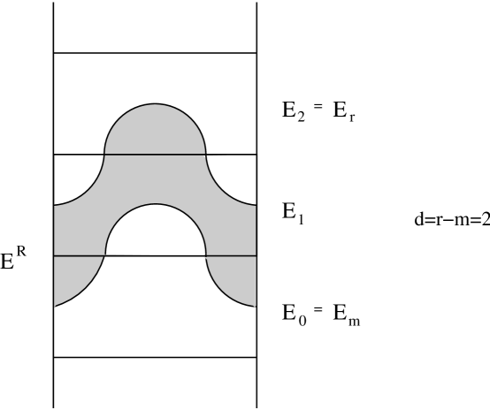
Definition 2.1.

Let $R$ be another spanning surface. Let $E^{R}$ be any lift of $E\setminus R$ to $\widetilde{E}$. We set

$$r=\max\{k\in{\mathbb{Z}}|E_{k}\text{ intersects }E^{R}\},\ m=\min\{k\in{\mathbb{Z}}|E_{k}\text{ intersects }E^{R}\}$$

and we put $d(S,R)=r-m$. This value does not depend on the choice of the lift $E^{R}$. See Figure 1.

Furthermore, for any two isotopy classes $\sigma,\rho$ of spanning surfaces we define $d(\sigma,\rho)$ to be the minimum of $d(S,R)$ over all representatives $S$ of $\sigma$ and $R$ of $\rho$.

Observe that in the case $\sigma=\rho$ we can take $S=R$ which satisfy $d(S,R)=0$. Recall that we declared two different vertices $\sigma,\rho$ of $MS(E,\gamma,\alpha)$ to be adjacent if they satisfy $d(S,R)=1$ for some $S\in\sigma,R\in\rho$. Note that if $S$ and $R$ are disconnected, it could happen that $S$ and $R$ are disjoint, but $d(S,R)$ exceeds $1$. One might not be able to improve that by varying $S$ and $R$ in the isotopy classes.

Kakimizu proves the following. (Our context is more general, but the proof trivially carries over.)

Proposition 2.2 ([K, Proposition 1.4]).

The function $d$ is a metric on $\mathcal{MS}(E,\gamma,\alpha)$.

In fact, if we endow the $1$–skeleton of $MS(E,\gamma,\alpha)$ with the path-metric $l$ in which all the edges have length $1$, then $d$ satisfies the following.

Proposition 2.3 ([K, Proposition 3.1]).

The metric $d$ coincides with $l$ on $\mathcal{MS}(E,\gamma,\alpha)$.

Let us indicate how Kakimizu proves Proposition 2.3. The distance $l=l(\sigma,\rho)$ is realised by a path $\sigma_{0}=\sigma,\sigma_{1},\ldots,\sigma_{l}=\rho$. By Proposition 2.2, we have $d(\sigma,\rho)\leq d(\sigma_{0},\sigma_{1})+\ldots+d(\sigma_{l-1},\sigma_{l})=l$, which is the estimate in one direction. The second estimate will be explained at the beginning of Section 4.

3 Simplified intersection

In this section we address the following issue. What hypotheses on the representatives $S,R$ of spanning surfaces $\sigma,\rho$ guarantee $d(\sigma,\rho)=d(S,R)$? To formulate a criterion we need the following terminology (see [O]).

Let $S,R$ be compact surfaces properly embedded in a connected (not necessarily compact) $3$–manifold $M$ with boundary. We discuss product regions bounded by $S$ and $R$ in $\partial M$ and $M$. If $\beta$ is an (abstract) arc, we denote by $\mathfrak{I}$ the product $\beta\times I$ with $\{x\}\times I$ collapsed to a point for each $x\in\partial\beta$. A product region in $\partial M$ is an embedded copy of $\mathfrak{I}$ with $\beta\times\{0\}\subset S,\ \beta\times\{1\}\subset R$, and $\mathfrak{I}\cap(S\cup R)=\partial\mathfrak{I}$. Similarly, if $W$ is a compact surface with boundary and $\delta$ is a closed $1$–submanifold of $\partial W$, we denote by $\mathfrak{J}$ the product $W\times I$ with intervals $\{x\}\times I$ collapsed to points for $x\in\delta$. A product region in $M$ (called a blister in [Sa]) is an embedded copy of $\mathfrak{J}$ with $W\times\{0\}\subset S,\ W\times\{1\}\subset R$, and $\mathfrak{J}\cap(S\cup R)=\partial\mathfrak{J}\setminus\text{int}(\mathfrak{J}\cap\partial M)$. Note that $\delta$ is allowed to be empty, in which case the product region is really a product.

We say that two surfaces $S,R$ in a manifold $M$ have simplified intersection, if they do not bound any product region. In particular, if a component $\dot{S}$ of $S$ is isotopic to a component $\dot{R}$ of $R$, then we must have $\dot{S}=\dot{R}$.

We say that $S$ and $R$ are almost transverse if for each component $\dot{S}$ of $S$ and $\dot{R}$ of $R$ either $\dot{S}$ equals $\dot{R}$ or they intersect transversely. In particular, if $S$ equals $R$ then $S$ and $R$ are almost transverse.

We say that surfaces $S$ and $R$ are almost disjoint if for intersecting components $\dot{S}$ of $S$ and $\dot{R}$ of $R$ we have $\dot{S}=\dot{R}$. In particular, $S$ is almost disjoint from itself.

Note that for a pair of surfaces $S,R$, the surface $R$ can be always isotoped to $R^{\prime}$ which is almost transverse to $S$ and has simplified intersection with $S$. (This is not true if we wanted to drop ‘almost‘, consider the case where some components of $S$ and $R$ coincide. Actually, this also fails in the very special case where $S=R$ and $M$ is a surface bundle over a circle, but we will ignore that since then $MS(E,\gamma,\alpha)$ is trivial.) Moreover, if $R_{1},R_{2}$ are almost disjoint, then they can be isotoped to almost disjoint $R_{1}^{\prime},R_{2}^{\prime}$ which are both almost transverse to $S$ and have simplified intersection with $S$ (again we cannot require that $R_{1}^{\prime},R_{2}^{\prime}$ are disjoint, even if $R_{1},R_{2}$ are).

Remark 3.1.

In [O] the definition of having simplified intersection consists of one more condition, which under standard hypotheses follows from the others. Namely, let $M$ be orientable, irreducible, $\partial$–irreducible and suppose that $S,R$ are orientable, incompressible and $\partial$–incompressible. If $S$ and $R$ are almost transverse and have simplified intersection, then there are no components of $S\cap R$ which are closed curves that are trivial in $S$ or $R$, or arcs that are $\partial$–parallel in $S$ or $R$.

We now answer the opening question of the section.

Proposition 3.2.

Let $S,R$ be spanning surfaces in $E$ representing $\sigma,\rho$ in $\mathcal{MS}(E,\gamma,\alpha)$. If $S$ and $R$ are almost transverse and have simplified intersection, then they satisfy

$$d(\sigma,\rho)=d(S,R).$$

We deduce Proposition 3.2 from the following version of [Sa, Proposition 4.8(2)], which we give without a proof.

Proposition 3.3.

Let $M$ be (possibly non-compact) orientable, irreducible, and $\partial$–irreducible $3$–manifold. Let $W,N$ be (possibly non-compact) proper $3$–submanifolds of $M$ such that $\partial W,\partial N$ are incompressible and $\partial$–incompressible surfaces which are almost transverse with simplified intersection. If $N$ is isotopic to a submanifold $N^{\prime}$ such that the interior of $N^{\prime}$ is disjoint from $W$, then also the interior of $N$ is disjoint from $W$.

In the setting described in Section 2, this yields the following.

Corollary 3.4.

Let $W,N$ be proper $3$–submanifolds of $\widetilde{E}$ such that $\partial W,\partial N$ are unions of lifts of minimal genus spanning surfaces which are almost transverse with simplified intersection. If $N$ is isotopic to $N^{\prime}$ such that the interior of $N^{\prime}$ is disjoint from $W$, then also the interior of $N$ is disjoint from $W$.

We will usually invoke Corollary 3.4 in the situation where $W=\overline{E}_{j}$ and $N=\tau^{i}(\overline{E}^{R})$ for some $j,i$, where $E_{j}$ and $E^{R}$ are as in Section 2.

We are now prepared for the following.

Proof of Proposition 3.2..

Let $R$ and $S$ be almost transverse with simplified intersection. Let $R^{\prime}$ be an element of $\rho=[R]$ for which the minimum of $d(S,R^{\prime})$ is attained. Then we have $d(\sigma,\rho)=d(S,R^{\prime})=r^{\prime}-m^{\prime},$ where $E^{R^{\prime}},r^{\prime},m^{\prime}$ are as in Definition 2.1 with $R$ replaced by $R^{\prime}$. Then $E^{R^{\prime}}$ is disjoint from all $E_{j}$ with $j\geq r^{\prime}+1$ or $j\leq m^{\prime}-1$. Let $E^{R}$ be the lift of $E\setminus R$ to $\widetilde{E}$ isotopic to $E^{R^{\prime}}$. Since $R$ has simplified intersection with $S$, its lifts have simplified intersection with the lifts of $S$. By Corollary 3.4, $E^{R}$ is disjoint from all $E_{j}$ with $j\geq r^{\prime}+1$ or $j\leq m^{\prime}-1$. Then we have $r\leq r^{\prime}$ and $m\geq m^{\prime}$, which implies $d(S,R)\leq d(S,R^{\prime})$, as desired. ∎

We conclude with recording the following lemma, whose proof we leave for the reader.

Lemma 3.5.

Let $M$ be orientable, irreducible, $\partial$–irreducible and suppose that $S,R$ and $T$ are orientable, incompressible and $\partial$–incompressible surfaces properly embedded in $M$. Then $S,R$ and $T$ can be isotoped to be pairwise almost transverse and have pairwise simplified intersection.

4 Projection map

In this section we recall a construction of Kakimizu which we think of as a projection map and which will be our main tool. First, we need to fix a basepoint $\sigma\in\mathcal{MS}(E,\gamma,\alpha)$. The projection map $\pi_{\sigma}$ will map every $\rho\in\mathcal{MS}(E,\gamma,\alpha)$ at distance $n>0$ from $\sigma$ to a vertex $\pi_{\sigma}(\rho)\in\mathcal{MS}(E,\gamma,\alpha)$ adjacent to $\rho$ at distance $n-1$ from $\sigma$.

The existence of such projection map completes Kakimizu‘s proof of Proposition 2.3. It implies, in particular, that $MS(E,\gamma,\alpha)$ is connected. In the present article we promote this method to prove contractibility of $MS(E,\gamma,\alpha)$.

We say that an oriented surface $T$ is obtained by a cut-and-paste operation on $S$ and $R$ if it is a union of closures of oriented components of $S\setminus R,\ R\setminus S$ and common components of $S$ and $R$, with $\partial T\subset\partial S\cup\partial R$.

Definition 4.1.

Let $\sigma\neq\rho$ be vertices of $MS(E,\gamma,\alpha)$. Put $n=d(\sigma,\rho)$. For any fixed spanning surface $S\in\sigma$ we can choose $R\in\rho$ such that $S$ and $R$ are almost transverse with simplified intersection. In particular $S$ and $R$ have almost disjoint boundaries, which means that the boundary components are disjoint or equal. By Proposition 3.2 we have $d(S,R)=n$.

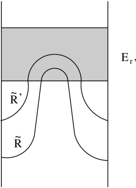
Recall the notation of Section 2 that $r$ is largest such that the translate $E_{r}$ of $E_{0}$ intersects the lift $E^{R}$ of $E\setminus R$ to $\widetilde{E}$. Denote $\widetilde{R}=\overline{E}^{R}\cap\tau(\overline{E}^{R})$. Let $\widetilde{P}\subset S_{r}\cup\widetilde{R}$ denote the surface obtained by a cut-and-paste operation on $S_{r}$ and $\widetilde{R}$, which is the intersection of the boundaries of $\overline{E}^{R}\setminus E_{r}$ and $\tau(\overline{E}^{R})\cup\overline{E}_{r}$. See Figure 2.

Figure 2: Construction of $\widetilde{P}$

The surface $\widetilde{P}$ considered with the orientation inherited from $\widetilde{R}$ and $S_{r}$ satisfies in homology $\partial(E^{R}\cap E_{r})=\widetilde{R}-\widetilde{P}$. Hence the image $P$ of $\widetilde{P}$ under $p$ is in the homology class $\alpha$. Moreover, $\widetilde{P}$ embeds under $p$ into $E$. In order to justify that $P$ is a spanning surface, it remains to prove that its boundary $\partial P$ is not only homological but also homotopic to $\gamma$. This follows from the fact that $\partial P$ is homotopic to a combination of curves in $\gamma$ and that by the hypothesis that $\gamma$ does not separate the components of $\partial E$ no non-trivial combination of curves in $\gamma$ is homological to zero.

Now a calculation as in case 1 of the proof of [K, Theorem 2.1] yields that $P$ is a spanning surface of minimal genus. We define

$$\pi_{\sigma}(\rho)=[P].$$

We prove that this class is well-defined in Proposition 4.4.

As indicated at the beginning of this section, we have the following property, which justifies calling $\pi_{\sigma}$ the projection.

Remark 4.2.

The surface $P$ in Definition 4.1 satisfies $d(R,P)=1$ and $d(S,P)=n-1$. Hence $\pi_{\sigma}(\rho)$ is adjacent to $\rho$ and satisfies $d(\sigma,\pi_{\sigma}(\rho))=n-1$.

In the proof that the projection is well-defined we need the following result.

Theorem 4.3 ([O, Theorem 3]).

Let $M$ be an orientable, irreducible, $\partial$–irreducible $3$–manifold. Let $S,R$ be orientable, incompressible, $\partial$–incompressible surfaces properly embedded in $M$. Assume that $S$ and $R$ are almost transverse with simplified intersection and that they are isotopic to $S^{\prime},R^{\prime},$ respectively, which are also almost transverse with simplified intersection. Suppose a cut-and-paste operation on $S$ and $R$ yields an orientable, incompressible and $\partial$–incompressible surface $P$. Then there is a corresponding cut-and-paste operation on $S^{\prime},R^{\prime}$ yielding a surface $P^{\prime}$ isotopic to $P$.

Proposition 4.4.

The class $[P]$ in Definition 4.1 does not depend on the choice of $S$ and $R$.

Proof.

We can fix $S\in\sigma$. Let $R,R^{\prime}\in\rho$ be almost transverse to $S$ with simplified intersection. Let $\widetilde{P}$ be obtained by a cut-and-paste operation on $\widetilde{R}$ and $S_{r}$ as in Definition 4.1. Let $E^{R^{\prime}},\ \widetilde{R}^{\prime}$ be the lifts of $E\setminus R^{\prime},\ R^{\prime}$ to $\widetilde{E}$ isotopic to $E^{R},\ \widetilde{R},$ respectively. By Corollary 3.4, $r$ is the largest integer such that $E^{R^{\prime}}$ intersects $E_{r}$. Let $\widetilde{P}^{\prime}$ be the surface obtained from the cut-and-paste operation on $S_{r}$ and $\widetilde{R}^{\prime}$ described in Definition 4.1, with $\widetilde{R}^{\prime}$ in place of $\widetilde{R}$.

By Theorem 4.3 there is a surface $\widetilde{P}^{\prime\prime}$, obtained by a cut-and-paste operation on $\widetilde{R}^{\prime}$ and $S_{r}$, which is isotopic to $\widetilde{P}$. The correspondence in Theorem 4.3 (arising from the proof) is such that in fact we have $\widetilde{P}^{\prime\prime}=\widetilde{P}^{\prime}$, as desired. ∎

5 Ordering the vertices

In this section we describe a natural way of ordering the vertices of the complex $MS(E,\gamma,\alpha)$. One can check that for special arborescent links this order coincides with the order described in [Sa, Lemma 3.7] (for appropriate $\sigma$).

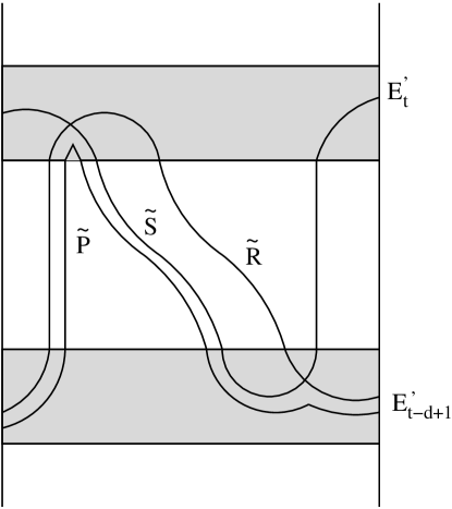
We begin with the following, which describes a possible position of a pair of adjacent vertices $\rho,\rho^{\prime}\in\mathcal{MS}(E,\gamma,\alpha)$ with respect to a vertex $\sigma\in\mathcal{MS}(E,\gamma,\alpha)$. Note that $\rho$ and $\rho^{\prime}$ may be at the same or different distance from $\sigma$. We may choose almost disjoint $R\in\rho,R^{\prime}\in\rho^{\prime}$ such that $R$ and $R^{\prime}$ are almost transverse to a fixed $S\in\sigma$ and have simplified intersection with $S$. Moreover, we can assume that $R$ and $R^{\prime}$ have also simplified intersection (this does not follow automatically from almost disjointness). By Proposition 3.2 we then have $d(R,R^{\prime})=1$. As usual $E^{R^{\prime}}$ denotes a lift of $E\setminus R^{\prime}$ to $\widetilde{E}$ and $r^{\prime}$ is largest such that $E_{r^{\prime}}$ intersects $E^{R^{\prime}}$. Let $E^{R}$ be the lift of $E\setminus R$ contained in $\overline{E}^{R^{\prime}}\cup\tau^{-1}(\overline{E}^{R^{\prime}})$.

Definition 5.1.

If $E^{R}$ intersects $E_{r^{\prime}}$, then we write

$$\rho<_{\sigma}\rho^{\prime}.$$

See Figure 3. We write $\rho\leq_{\sigma}\rho^{\prime}$ if $\rho<_{\sigma}\rho^{\prime}$ or $\rho=\rho^{\prime}$.

Figure 3: Relation $[R]<_{\sigma}[R^{\prime}]$

Remark 5.2.

Definition 5.1 does not depend on the choices of $R$ and $R^{\prime}$. Indeed, by Corollary 3.4 the isotopy class of $E^{R^{\prime}}$ does not depend on the choice of $R^{\prime}\in\rho^{\prime}$. Hence also the isotopy class of $E^{R}$ is well-defined. Again by Corollary 3.4 the property that $E^{R}$ intersects $E_{r^{\prime}}$ is invariant.

We prove that adjacent vertices are always related by $<_{\sigma}$.

Lemma 5.3.

Let $\rho\neq\rho^{\prime}$ be adjacent vertices of $MS(E,\gamma,\alpha)$ and consider any $\sigma\in\mathcal{MS}(E,\gamma,\alpha)$. Then we have $\rho^{\prime}<_{\sigma}\rho$ or $\rho<_{\sigma}\rho^{\prime}$.

Later, in Lemma 5.5, we will show that in fact $\rho^{\prime}<_{\sigma}\rho$ and $\rho<_{\sigma}\rho^{\prime}$ cannot happen simultaneously, which justifies using the notation $<_{\sigma}$.

Proof.

Assume we do not have $\rho<_{\sigma}\rho^{\prime}$, i.e. $E^{R}$ is disjoint from $E_{r^{\prime}}$. If we now interchange $\rho$ with $\rho^{\prime}$, then $E_{r}=E_{r^{\prime}-1}$ takes on the role of $E_{r^{\prime}}$ and $\tau^{-1}(E^{R^{\prime}})$ takes on the role of $E^{R}$. Since $\tau^{-1}(E^{R^{\prime}})$ intersects $E_{r^{\prime}-1}$, we have $\rho^{\prime}<_{\sigma}\rho$. ∎

In the following configuration we can determine the direction of the relation $<_{\sigma}$.

Lemma 5.4.

If in Definition 5.1 the vertex $\rho$ is farther from $\sigma$ then $\rho^{\prime}$, then we have $\rho<_{\sigma}\rho^{\prime}$.

Proof.

Since $E^{R}$ is contained in $\overline{E}^{R^{\prime}}\cup\tau^{-1}(\overline{E}^{R^{\prime}})$, it may intersect only $E_{k}$ with $m^{\prime}-1\leq k\leq r^{\prime}$. By Proposition 3.2 we have $d(S,R)=d(S,R^{\prime})+1$, so $E^{R}$ must intersect all those $E_{k}$. In particular it intersects $E_{r^{\prime}}$, as desired. ∎

We now prove that, in particular, $\rho^{\prime}\leq_{\sigma}\rho$ and $\rho\leq_{\sigma}\rho^{\prime}$ implies $\rho=\rho^{\prime}$.

Lemma 5.5.

There are no $\rho^{1},\ldots,\rho^{k},$ for $k\geq 2,$ satisfying

$$\rho^{1}<_{\sigma}\rho^{2}<_{\sigma}\ldots<_{\sigma}\rho^{k}<_{\sigma}\rho^{1}.$$

Before we provide the proof, we record the following immediate consequence. Note that in general the relation $<_{\sigma}$ is not transitive, because $\rho<_{\sigma}\rho^{\prime}$ and $\rho^{\prime}<_{\sigma}\rho^{\prime\prime}$ do not imply that $\rho$ and $\rho^{\prime\prime}$ are adjacent.

Corollary 5.6.

The relation $<_{\sigma}$ extends to a linear order on $\mathcal{MS}(E,\gamma,\alpha)$.

Proof of Lemma 5.5.

Since consecutive $\rho^{i}$ are adjacent, we can inductively choose $R^{k}\in\rho^{k},R^{k-1}\in\rho^{k-1},\ldots,R^{1}\in\rho^{1}$ satisfying the following. First, each $R^{i}$ is almost transverse to $S$ with simplified intersection. Second, for $i<k$ the surface $R^{i}$ is almost disjoint with $R^{i+1}$ and they have simplified intersection. Let $r$ be largest such that $E_{r}$ intersects a lift $E^{R^{k}}$ of $E\setminus R^{k}$. For $i<k$ define inductively $E^{R^{i}}$ to be the lift of $E\setminus R^{i}$ contained in $\overline{E}^{R^{i+1}}\cup\tau^{-1}(\overline{E}^{R^{i+1}})$. In view of $\rho^{1}<_{\sigma}\rho^{2}<_{\sigma}\ldots<_{\sigma}\rho^{k},$ all $E^{R^{i}}$ intersect $E_{r}$.

Finally, let $R^{*}\in\rho^{k}$ be almost transverse to $S$ with simplified intersection and almost disjoint from $R^{1}$ with simplified intersection. Let $E^{R^{*}}$ be the lift of $E\setminus R^{*}$ contained in $\overline{E}^{R^{1}}\cup\tau^{-1}(\overline{E}^{R^{1}})$. In view of $\rho^{k}<_{\sigma}\rho^{1}$, $E^{R^{*}}$ intersects $E_{r}$. By Corollary 3.4, $E^{R^{*}}$ and $E^{R^{1}}$ lie in the same isotopy class. Then the surfaces $\overline{E}^{R^{*}}\cap\tau(\overline{E}^{R^{*}})$ and $\overline{E}^{R^{1}}\cap\tau(\overline{E}^{R^{1}})$ are almost disjoint and bound a product containing all $\overline{E}^{R^{i}}\cap\tau(\overline{E}^{R^{i}})$. Hence all $\rho_{i}$ coincide, contradiction. ∎

6 Properties of the projection map

In this section we collect the properties of the projection map which will be later used to prove the theorems from the Introduction.

The following property of the projection map $\pi_{\sigma}$ is the key to our proof of Theorem 1.1.

Lemma 6.1.

Let $\rho$ and $\rho^{\prime}$ be adjacent vertices of $MS(E,\gamma,\alpha)$ such that $\rho$ is different from some $\sigma\in\mathcal{MS}(E,\gamma,\alpha)$. Assume $\rho\leq_{\sigma}\rho^{\prime}$. Then we have $\rho^{\prime}\leq_{\sigma}\pi_{\sigma}(\rho)$. In particular $\pi_{\sigma}(\rho)$ and $\rho^{\prime}$ are equal or adjacent.

Proof.

Let $S,R,R^{\prime},E^{R^{\prime}},E^{R}$ be as in Definition 5.1 and let $\widetilde{P}$ be as in Definition 4.1. Let $E^{P}$ be that lift of $E\setminus P$ which contains $E^{R}\setminus E_{r}$.

Then $E^{R^{\prime}}$ is contained in $\overline{E}^{P}\cup\tau(\overline{E}^{P})$. In particular $\pi_{\sigma}(\rho)$ and $\rho^{\prime}$ are equal or adjacent. There is an isotopy $i$ of $P$ such that $i(P)$ is almost transverse to $S$ with simplified intersection and almost disjoint with $R^{\prime}$ with simplified intersection. Since $E^{P}$ is disjoint from $E_{r}$, by Corollary 3.4 so is the lift of $E\setminus i(P)$ in the isotopy class of $E^{P}$. Hence we do not have $\pi_{\sigma}(\rho)<_{\sigma}\rho^{\prime}$. By Lemma 5.3 we then have $\rho^{\prime}\leq_{\sigma}\pi_{\sigma}(\rho)$, as desired. See Figure 4. ∎

Figure 4: Configuration from Lemma 6.1

A double application of Lemma 6.1 yields the following.

Corollary 6.2.

Let $\rho$ and $\rho^{\prime}$ be adjacent vertices of $MS(E,\gamma,\alpha)$ different from some $\sigma\in\mathcal{MS}(E,\gamma,\alpha)$. Assume $\rho\leq_{\sigma}\rho^{\prime}$. Then we have $\pi_{\sigma}(\rho)\leq_{\sigma}\pi_{\sigma}(\rho^{\prime})$.

The following two results will be only used in the proof of Theorem 1.2 in Section 8. They are inspired by [Pol]. In particular the proof of our Lemma 6.4 resembles the proof of [Pol, Lemma 3.9].

Figure 5: Configuration from Lemma 6.3

Lemma 6.3.

Assume that there are vertices $\rho^{1},\ldots,\rho^{k}$ at the same non-zero distance from $\sigma\in\mathcal{MS}(E,\gamma,\alpha)$ satisfying

$$\rho^{1}<_{\sigma}\rho^{2}<_{\sigma}\ldots<_{\sigma}\rho^{k},\text{ and }\pi_{\sigma}(\rho^{1})=\pi_{\sigma}(\rho^{k}).$$

Then all $\pi_{\sigma}(\rho^{i})$ are equal and all $\rho^{i}$ are adjacent.

Proof.

The fact that all $\pi_{\sigma}(\rho^{i})$ are equal follows immediately from Corollary 6.2 and Lemma 5.5. To show that all $\rho^{i}$ are adjacent it is enough to give an argument that $\rho^{1}$ and $\rho^{k}$ are adjacent (for other pairs of $\rho^{i}$ we pass to a subsequence).

First we choose $E^{R^{k}},\ldots,E^{R^{1}}$ in the same way as in the proof of Lemma 5.5. Let $\widetilde{P}^{1},\widetilde{P}^{k}$ be obtained as in Definition 4.1. Then $\tau(\widetilde{P}^{k})$ is disjoint from $E^{R^{k}}$ and in the same isotopy class as $\tau(\widetilde{P}^{1})$. See Figure 5. Hence $\widetilde{R}^{1}$ and $\widetilde{R}^{k}$ are isotopic to almost disjoint surfaces $i(\widetilde{R}^{1})$ and $i(\widetilde{R}^{k})$ contained in the closure of the lift of $E\setminus P$ bounded by $\widetilde{P}^{1}$ and $\tau(\widetilde{P}^{1})$. Then we have

$$d\big{(}p(i(\widetilde{R}^{1})),p(i(\widetilde{R}^{k}))\big{)}=1.$$

∎

Recall that by [Sa, Proposition 4.9(1)] all simplices of $MS(E,\gamma,\alpha)$ can be realised by sets of disjoint spanning surfaces. Hence by Kneser‘s theorem, there is a bound on the dimension of simplices in $MS(E,\gamma,\alpha)$. We promote this to the following.

Lemma 6.4.

For any $n>0$ there is a constant $l_{n}$ satisfying the following. Let $\sigma$ be any vertex of $MS(E,\gamma,\alpha)$ and let $\rho^{1},\ldots,\rho^{l}$ be at distance $n$ from $\sigma$ satisfying

$$\rho^{1}<_{\sigma}\rho^{2}<_{\sigma}\ldots<_{\sigma}\rho^{l}.$$

Then we have $l\leq l_{n}$.

Proof.

Let $L$ be a bound on the dimension of simplices in $MS(E,\gamma,\alpha)$. We prove by induction that it suffices to put $l_{n}=(L+1)^{n}$. For $n=1$ this follows directly from Lemma 6.3. Assume we have verified this for some $n\geq 1$.

Let now $\rho^{1},\ldots,\rho^{l}$ be at distance $n+1$ from $\sigma$ satisfying $\rho^{1}<_{\sigma}\rho^{2}<_{\sigma}\ldots<_{\sigma}\rho^{l}$. Put $i_{0}=0$. For $k\geq 1$ define inductively $i_{k}$ to be maximal satisfying $\pi_{\sigma}(\rho^{i_{k}})=\pi_{\sigma}(\rho^{i_{k-1}+1})$, until some $i_{m}$ equals $l$. By Lemma 6.3 for all $1\leq k\leq m$ we have $i_{k}-i_{k-1}\leq L+1$. Summing up this implies $l\leq m(L+1)$.

It remains to bound $m$. By Corollary 6.2 for all $1\leq k<m$ we have $\pi_{\sigma}(\rho^{i_{k}})<_{\sigma}\pi_{\sigma}(\rho^{i_{k}+1})$. This gives rise to

$$\pi_{\sigma}(\rho^{i_{1}})<_{\sigma}\pi_{\sigma}(\rho^{i_{2}})<_{\sigma}\ldots<_{\sigma}\pi_{\sigma}(\rho^{i_{m}}).$$

By Remark 4.2, all $\pi_{\sigma}(\rho^{i_{k}})$ are at distance $n$ from $\sigma$. By induction hypothesis we have $m\leq l_{n}$. Altogether, $l$ is bounded by $l_{n+1}=l_{n}(L+1)$, as desired. ∎

We will also need in Section 8 the following technical result. Roughly speaking it says that projection paths do not exit balls containing their endpoints.

Lemma 6.5.

For $\sigma\neq\rho,\sigma^{\prime}\in\mathcal{MS}(E,\gamma,\alpha)$ with $d(\sigma^{\prime},\rho)\leq d$ and $d(\sigma^{\prime},\sigma)\leq d$ we have $d(\sigma^{\prime},\pi_{\sigma}(\rho))\leq d$.

Proof.

Choose $S\in\sigma,R\in\rho,S^{\prime}\in\sigma^{\prime}$ which are pairwise almost transverse with simplified intersection (see Lemma 3.5). Let $r,\widetilde{P},P$ be as in Definition 4.1. Let $E^{P}$ be the lift of $E\setminus P$ bounded by $\widetilde{P}$ and $\tau^{-1}(\widetilde{P})$. Choose a lift $E^{\prime}_{0}$ of $E\setminus S^{\prime}$ to $\widetilde{E}$ and denote $E^{\prime}_{k}=\tau^{k}(E^{\prime}_{0})$.

Figure 6: Configuration from Lemma 6.5 (here $\widetilde{S}=\overline{E}_{r}\cap\overline{E}_{r+1}$)

Let $t$ be largest such that $E^{\prime}_{t}$ intersects $E^{R}\cap E_{r-1}$ (which is non-empty). Note (see Figure 6) that $E^{P}$ is contained in the union of

$$E^{R}\cap\big{(}\bigcup_{k\leq r-1}\overline{E}_{k}\big{)}\text{ and }E_{r-1}\cap\big{(}\bigcup_{i\leq 0}\tau^{i}(\overline{E}^{R})\big{)}.$$

In particular, $E^{P}$ is contained in the intersection of $E^{R}\cup E_{r-1}$ with $\overline{E}^{\prime}_{k}$‘s satisfying $k\leq t$. Since we have $d(S^{\prime},R)\leq d$ and $d(S^{\prime},S)\leq d$, these $k$ must satisfy $t-k\leq d$, as desired. ∎

We conclude with another technical lemma which will be used only in Section 9. Roughly speaking, it describes how does the projection $\pi_{\sigma^{\prime}}$ look from the point of view of a vertex $\sigma$ adjacent to $\sigma^{\prime}$.

Lemma 6.6.

Let $\sigma,\sigma^{\prime}\in\mathcal{MS}(E,\gamma,\alpha)$ be adjacent. Let $\rho,\rho^{\prime}\in\mathcal{MS}(E,\gamma,\alpha)$ be also adjacent satisfying $\rho^{\prime}<_{\sigma^{\prime}}\rho$ and $\rho<_{\sigma}\rho^{\prime}$. If $\sigma^{\prime}\neq\rho^{\prime}$, then we have

1. $\rho\leq_{\sigma}\pi_{\sigma^{\prime}}(\rho^{\prime})$,

2. if $\sigma\neq\rho^{\prime}$, then $d(\sigma,\pi_{\sigma^{\prime}}(\rho^{\prime}))\leq d(\sigma,\rho^{\prime})$.

See Figure 7 for an illustration.

Figure 7: Configuration from Lemma 6.6 (here $\widetilde{S}=\overline{E}_{r^{\prime}}\cap\overline{E}_{r^{\prime}+1}$ and $\widetilde{S}^{\prime}=\overline{E}^{\prime}_{r^{\prime}}\cap\overline{E}^{\prime}_{r^{\prime}+1}$)

Proof.

Let $S\in\sigma,S^{\prime}\in\sigma^{\prime},R\in\rho,R^{\prime}\in\rho^{\prime}$ be pairwise almost transverse with simplified intersection (this is easily achieved by viewing $S\cup S^{\prime}$ and $R\cup R^{\prime}$ as a pair of surfaces). Let $E_{0}^{\prime}$ be the lift of $E\setminus S^{\prime}$ contained in $\overline{E}_{0}\cup\overline{E}_{1}$ (for some lift $E_{0}$ of $E\setminus S$). Let $r^{\prime}$ be largest such that $E^{\prime}_{r^{\prime}}=\tau^{r^{\prime}}(E^{\prime}_{0})$ intersects a lift $E^{R^{\prime}}$ of $E\setminus R^{\prime}$. Let $E^{R}$ be the lift of $E\setminus R$ contained in $\overline{E}^{R^{\prime}}\cup\tau^{-1}(\overline{E}^{R^{\prime}})$.

The hypotheses $\rho^{\prime}<_{\sigma^{\prime}}\rho$ and $\rho<_{\sigma}\rho^{\prime}$ guarantee that $E^{R}$ is disjoint from $E^{\prime}_{r^{\prime}}$ but intersects $E_{r^{\prime}}$. Let $P^{\prime}=p(\widetilde{P}^{\prime})\in\pi_{\sigma^{\prime}}(\rho^{\prime})$ be obtained as in Definition 4.1 and let $E^{P^{\prime}}$ be the lift of $E\setminus{P^{\prime}}$ bounded by $\widetilde{P}^{\prime}$ and $\tau^{-1}(\widetilde{P}^{\prime})$. Since $E^{R}$ is disjoint from $E^{\prime}_{r^{\prime}}$, the surface $\widetilde{P}^{\prime}$ is contained in $\tau(\overline{E}^{R})$. (In particular $\rho$ and $\pi_{\sigma^{\prime}}(\rho^{\prime})$ are equal or adjacent.)

There is an isotopy $i$ of $P^{\prime}$ such that $i(P^{\prime})$ is almost transverse to $S$ with simplified intersection and almost disjoint from $R$ with simplified intersection. Since $E^{P^{\prime}}$ is disjoint from $E_{r^{\prime}+1}$, by Corollary 3.4 so is the lift of $E\setminus i(P^{\prime})$ in the isotopy class of $E^{P^{\prime}}$. Moreover, this lift contains $\widetilde{R}$ which intersects $E_{r^{\prime}}$. This implies assertion (i).

Assertion (ii) is trivial since $E^{P^{\prime}}$ intersects exactly the same $E_{k}$ as $E^{R^{\prime}}$. ∎

7 Contractibility

In this section we prove Theorem 1.1. By Whitehead‘s theorem it suffices to prove that all finite subcomplexes of $MS(E,\gamma,\alpha)$ are contained in contractible subcomplexes of $MS(E,\gamma,\alpha)$.

We say that a flag subcomplex $X\subset MS(E,\gamma,\alpha)$ is $\sigma$–convex, for $\sigma\in X^{(0)}$, if for any $\rho\neq\sigma\in X^{(0)}$ we have $\pi_{\sigma}(\rho)\in X^{(0)}$. By Remark 4.2 each finite subcomplex of $MS(E,\gamma,\alpha)$ is contained in a finite $\sigma$–convex subcomplex of $MS(E,\gamma,\alpha)$ for any (hence some) $\sigma$. Hence in order to prove Theorem 1.1, it suffices to establish that finite $\sigma$–convex subcomplexes of $MS(E,\gamma,\alpha)$ are contractible. In fact, we have even a stronger property than contractibility.

Definition 7.1.

A finite graph is dismantlable if its vertices can be linearly ordered $x_{0},\ldots,x_{m}$ so that for each $i\neq m$ there is $j>i$ satisfying

1. the vertex $x_{j}$ is adjacent to $x_{i}$,

2. for any $x_{k}$ adjacent to $x_{i}$ with $k>i$, the vertex $x_{j}$ is adjacent or equal to $x_{k}$.

It is well known that finite flag complexes whose $1$–skeleta are dismantlable are contractible (see e.g. [CO]). We just indicate that one obtains a homotopy retraction onto $x_{m}$ by successively retracting $x_{i}$ to $x_{j}$, where $j$ is as in Definition 7.1. In view of this in order to prove Theorem 1.1 it remains to prove the following.

Theorem 7.2.

Finite $\sigma$–convex subcomplexes of $MS(E,\gamma,\alpha)$ have dismantlable $1$–skeleta.

Proof.

We order all the vertices by extending the relation $<_{\sigma}$, which is possible by Corollary 5.6. By Lemma 6.1 for all $\rho\neq\sigma$ we have $\rho<_{\sigma}\pi_{\sigma}(\rho)$, hence $\sigma$ is largest in this order.

For any non-largest $x_{i}$ we put $x_{j}=\pi_{\sigma}(x_{i})$. As discussed above we have $x_{i}<_{\sigma}x_{j}$, which implies $j>i$ and condition (i) in Definition 7.1.

It remains to verify condition (ii). Let $x_{k}$ be adjacent to $x_{i}$ with $k>i$. By Lemma 5.3 we have $x_{i}<_{\sigma}x_{k}$ or $x_{k}<_{\sigma}x_{i}$. Since $k>i$ we must have $x_{i}<_{\sigma}x_{k}$. Then $x_{j}$ and $x_{k}$ are adjacent or equal by Lemma 6.1. ∎

8 Fixed-point theorem

In this section we prove Theorem 1.2. Key notions will be the following.

Definition 8.1.

A flag subcomplex $X$ of $MS(E,\gamma,\alpha)$ is convex if for all $\sigma\neq\rho\in X^{(0)}$ the vertex $\pi_{\sigma}(\rho)$ lies in $X^{(0)}$.

For a vertex $v$ of $MS(E,\gamma,\alpha)$, let $N(v)$ denote the union of $v$ with the set of all vertices adjacent to $v$. For a subcomplex $X$ of $MS(E,\gamma,\alpha)$ we put $N_{X}(v)=N(v)\cap X^{(0)}$.

A flag subcomplex $X$ of $MS(E,\gamma,\alpha)$ is semi-convex if for all $\sigma\neq\rho\in X^{(0)}$ there exists a vertex $\pi\in X^{(0)}$ satisfying

$$N_{X}(\pi_{\sigma}(\rho))\subset N_{X}(\pi),$$

and such that the distance between $\pi$ and $\sigma$ in the $1$–skeleton of $X$ equals $d(\pi_{\sigma}(\rho),\sigma)$. In particular, a convex subcomplex is also semi-convex.

The convex hull of a subcomplex $X$ of $MS(E,\gamma,\alpha)$ is the minimal convex subcomplex of $MS(E,\gamma,\alpha)$ containing $X$, i.e. it is the intersection of all convex subcomplexes of $MS(E,\gamma,\alpha)$ containing $X$.

Note that semi-convex subcomplexes of $MS(E,\gamma,\alpha)$ have $1$–skeleta isometrically embedded in the $1$–skeleton of $MS(E,\gamma,\alpha)$. Hence when we discuss the distances in semi-convex subcomplexes we do not have to specify if we consider the distance in the $1$–skeleton of the subcomplex or of the whole $MS(E,\gamma,\alpha)$. We also need the following preliminary result which follows directly from Lemma 6.5.

Corollary 8.2.

The convex hull of a subcomplex of diameter $d$ (in the $1$–skeleton of $MS(E,\gamma,\alpha)$) has diameter $d$ as well.

Proof of Theorem 1.2.

Let $X\subset\mathcal{MS}(E,\gamma,\alpha)$ be a finite orbit of the $G$–action on $\mathcal{MS}(E,\gamma,\alpha)$. Denote by $\overline{X}$ the convex hull of $X$. By Corollary 8.2 $\overline{X}$ has finite diameter. Note that $\overline{X}$ is $G$–invariant. We consider now $G$–invariant non-empty semi-convex subcomplexes $Y$ of $MS(E,\gamma,\alpha)$ of minimal diameter $d$. We want to show that $d$ equals $1$.

Otherwise, we also minimise the following value $l(Y)$. It is the maximum over $\sigma\in Y^{(0)}$ of $l$ admitting a sequence $\rho^{1}<_{\sigma}\rho^{2}<_{\sigma}\ldots<_{\sigma}\rho^{l}$ for some $\rho^{1},\ldots,\rho^{l}$ at distance $d$ from $\sigma$. Note that $l(Y)$ is always finite by Lemma 6.4.

We say that a vertex $v$ of a subcomplex $Y$ of $MS(E,\gamma,\alpha)$ is strongly dominated (by $w$) in $Y$ if there is a vertex $w$ in $Y$ satisfying $N_{Y}(v)\subsetneq N_{Y}(w)$.

Let $Z$ denote the set of all the vertices $v\in Y^{(0)}$ strongly dominated in $Y$. Let $W$ be the subcomplex of $Y$ spanned by all the vertices in $Y^{(0)}\setminus Z$. Obviously $W$ is $G$–invariant. In order to obtain a contradiction it suffices to establish that $W$ is non-empty and semi-convex, and $l(W)<l(Y)$.

We first prove $l(W)<l(Y)$. Consider any $\sigma\in W^{(0)}$ and a sequence $\rho^{1}<_{\sigma}\rho^{2}<_{\sigma}\ldots<_{\sigma}\rho^{l(Y)}$ of vertices at distance $d$ from $\sigma$. It suffices to show that $\rho^{1}$ belongs to $Z$.

By the definition of $l(Y)$ every $\rho\in Y^{(0)}$ at distance $d$ from $\sigma$ adjacent to $\rho^{1}$ violates $\rho<_{\sigma}\rho^{1}$. Then by Lemma 5.3 we have $\rho^{1}<_{\sigma}\rho$. By Lemma 5.4 the same holds for all other $\rho\in Y^{(0)}$ adjacent to $\rho^{1}$. Hence by Lemma 6.1 all vertices in $Y$ adjacent to $\rho^{1}$ are adjacent to or equal $\pi_{\sigma}(\rho^{1})$. Note that $\pi_{\sigma}(\rho^{1})$ might note lie in $Y^{(0)}$ but since $Y$ is semi-convex, there is $\pi\in Y^{(0)}$ at distance $d-1$ from $\sigma$ satisfying $N_{Y}(\pi_{\sigma}(\rho^{1}))\subset N_{Y}(\pi)$. At this point we have

$$N_{Y}(\rho^{1})\subset N_{Y}(\pi).$$

Similarly, since $d\geq 2$, there is $\pi^{\prime}\in Y^{(0)}$ at distance $d-2$ from $\sigma$ satisfying $N_{Y}(\pi_{\sigma}(\pi))\subset N_{Y}(\pi^{\prime})$. In particular, $\pi^{\prime}$ is adjacent to $\pi$, but not to $\rho^{1}$. Hence we have

$$N_{Y}(\rho^{1})\subsetneq N_{Y}(\pi).$$

We conclude that $\rho^{1}$ is strongly dominated by $\pi$ in $Y$, which means that $\rho^{1}$ belongs to $Z$.

We now prove that $W$ is non-empty. Pick a vertex $v\in Y^{(0)}$ with maximal $N_{Y}(v)$ (with respect to inclusion). Such a vertex exists since otherwise we would have a simplex in $MS(E,\gamma,\alpha)$ of infinite dimension. Then $v$ is not strongly dominated in $Y$ by any vertex and hence $v$ belongs to $W^{(0)}$.

It remains to show that $W$ is semi-convex. Take $\sigma\neq\rho\in W^{(0)}$. Since $Y$ is semi-convex, there is a vertex $\pi$ of $Y^{(0)}$ at distance $d-1$ from $\sigma$ satisfying $N(\pi_{\sigma}(\rho))\subset N(\pi)$. Let $\pi^{\prime}$ be a vertex of $Y^{(0)}$ with maximal possible $N_{Y}(\pi^{\prime})$ containing $N_{Y}(\pi)$. Such a vertex exists since $MS(E,\gamma,\alpha)$ is finite-dimensional. Then $\pi^{\prime}$ is not strongly dominated in $Y$, hence $\pi^{\prime}$ belongs to $W^{(0)}$. Note that we also have $N_{Y}(\pi_{\sigma}(\rho))\subset N_{Y}(\pi^{\prime})$.

Now we prove that $\pi^{\prime}$ is at distance $d-1$ from $\sigma$ in $W^{(1)}$. Let $\pi_{0}=\pi,\pi_{1},\ldots,\pi_{d-1}=\sigma$ be a  path in $Y^{(0)}$ from $\pi$ to $\sigma$. Put $\pi_{0}^{\prime}=\pi^{\prime},\pi_{d-1}^{\prime}=\sigma$ and for all $0<i<d-1$ let $\pi_{i}^{\prime}$ be a vertex of $Y^{(0)}$ with maximal possible $N_{Y}(\pi_{i}^{\prime})$ containing $N_{Y}(\pi_{i})$. Like before, all $\pi_{i}^{\prime}$ belong to $W^{(0)}$. Moreover, since $\pi_{i}$ is adjacent to $\pi_{i+1}$, also $\pi_{i}^{\prime}$ is adjacent to $\pi_{i+1}$ and consequently $\pi_{i}^{\prime}$ is adjacent to $\pi^{\prime}_{i+1}$. Hence $\pi_{i}^{\prime}$ form a path and $\pi^{\prime}$ is at distance $d-1$ from $\sigma$ in $W^{(1)}$. Thus $W$ is semi-convex, as required.

To summarise, assuming $d\geq 2$ we proved that $Y$ contains non-empty semi-convex $G$–invariant $W$ with $l(W)<l(Y)$ (where $l(W)=0$ means that the diameter of $W$ is less than $d$). This contradicts the choice of $Y$. In case $d=1$, $Y$ is the desired $G$–invariant simplex. ∎

Note that the proof would be easier if we knew that $MS(E,\gamma,\alpha)$ is locally finite.

9 Contractibility of fixed-point sets

In this section we prove Theorem 1.5. This is an elaboration on the proof from Section 7.

Let $G$ be a subgroup of the mapping class group of $E$ fixing $\alpha$ and the homotopy class of $\gamma$. Its fixed-point set $\mathrm{Fix}_{G}(MS(E,\gamma,\alpha))$ has the following structure of a flag simplicial complex $X$. Its vertices can be identified with the set $V$ of minimal $G$–invariant simplices of $MS(E,\gamma,\alpha)$. Its edges are spanned on pairs vertices corresponding to simplices in $MS(E,\gamma,\alpha)$ spanning a common simplex.

We assume that $X=\mathrm{Fix}_{G}(MS(E,\gamma,\alpha))$ is non-empty, i.e. there is a vertex $\Sigma\in V$ of $X$ (a simplex of $MS(E,\gamma,\alpha)$) which is invariant under $G$. We need to prove that $X$ is contractible. The plan of the proof is the same as in Section 7. We will define a mapping $\Pi_{\Sigma}$ from $V\setminus\{\Sigma\}$ to $V$ which will play the role of $\pi_{\sigma}$. We will observe that each finite subcomplex of $X$ lies in a finite $\Sigma$–convex subcomplex of $X$. The proof will then reduce to proving dismantlability of $\Sigma$–convex subcomplexes of $X$.

Definition 9.1.

For $\Sigma\neq\Delta\in V$ we define $\Pi_{\Sigma}(\Delta)\in V$ in the following way. We choose a vertex $\sigma$ of the simplex $\Sigma$. We consider $\delta\in\Delta$ which is minimal with respect to the order $<_{\sigma}$. We define $\Pi_{\Sigma}(\Delta)$ to be the $G$–orbit of $\pi_{\sigma}(\delta)$. We still need to check that this is an element of $V$, i.e. a simplex in $MS(E,\gamma,\alpha)$. Note that since the relation $<_{\sigma}$ and the mapping $\pi_{\sigma}$ are $G$–equivariant, this definition does not depend on the choice of $\sigma$.

Lemma 9.2.

$\Pi_{\Sigma}(\Delta)$ spans a simplex of $MS(E,\gamma,\alpha)$. As a vertex of $X$ it is adjacent to $\Delta$. Furthermore, for $\sigma\in\Sigma,\delta\in\Delta$ as in Definition 9.1 and all $\pi\in\Pi_{\Sigma}(\Delta)$ we have

$$\delta\leq_{\sigma}\pi.$$

Proof.

Let $\sigma\in\Sigma$ and $\delta\in\Delta$ be as in Definition 9.1. By Lemma 6.1, for all $\delta^{\prime}\in\Delta$ we have $\delta^{\prime}\leq_{\sigma}\pi_{\sigma}(\delta)$. In particular, $\pi_{\sigma}(\delta)$ is adjacent or equal to all the vertices of $\Delta$.

Let now $\pi$ be any vertex of $\Pi_{\Sigma}(\Delta)$. By equivariance, $\pi$ is adjacent or equal to all the vertices of $\Delta$. Moreover, we have $\pi=\pi_{\sigma^{\prime}}(\delta^{\prime})$ for some $\sigma^{\prime}\in\Sigma,\delta^{\prime}\in\Delta$ satisfying $\delta^{\prime}<_{\sigma^{\prime}}\delta$. Now Lemma 6.6(i) implies $\delta\leq_{\sigma}\pi$.

Finally, by Lemma 6.1, $\pi_{\sigma}(\delta)$ and $\pi$ are adjacent or equal. ∎

We have the following analogue of Remark 4.2, which in particular implies that $\Pi_{\Sigma}(\Delta)$ is different from $\Delta$.

Lemma 9.3.

The sum of the distances between a vertex of $\Sigma$ and all the vertices of $\Pi_{\Sigma}(\Delta)$ is less than the corresponding sum for $\Sigma$ and $\Delta$.

Note that by equivariance the value in Lemma 9.3 does not depend on the choice of the vertex of $\Sigma$.

Proof.

Fix $\sigma\in\Sigma$ and let $\delta\in\Delta$ be minimal with respect to $<_{\sigma}$. By Remark 4.2 we have $d(\sigma,\pi_{\sigma}(\delta))<d(\sigma,\delta)$. All other vertices $\delta^{\prime}\in\Delta$ are in correspondence with vertices $\pi^{\prime}\in\Pi_{\Sigma}(\Delta)$ of the form $\pi_{\sigma^{\prime}}(\delta^{\prime})$ for some $\sigma^{\prime}\in\Sigma$. By Lemma 6.6(ii) we then have $d(\sigma,\pi^{\prime})\leq d(\sigma,\delta^{\prime})$. Summing up the inequalities yields the lemma. ∎

We now introduce a definition analogous to the one in Section 7.

Definition 9.4.

A flag subcomplex $Y$ of $X$ is $\Sigma$–convex, for $\Sigma\in Y^{(0)}$, if for any $\Delta\in Y^{(0)}\setminus\{\Sigma\}$ we have $\Pi_{\Sigma}(\Delta)\in Y^{(0)}$.

Note that by Lemma 9.3 each finite subcomplex of $X$ is contained in a finite $\Sigma$–convex subcomplex of $X$. Hence in order to prove Theorem 1.5, it remains to show the following.

Theorem 9.5.

Let $Y$ be a finite $\Sigma$–convex subcomplex of $X$. Then $Y^{(1)}$ is dismantlable.

Proof.

We choose any $\sigma\in\Sigma$. By Corollary 5.6 we can extend the relation $<_{\sigma}$ to a linear order on $\mathcal{MS}(E,\gamma,\alpha)$. Let $x_{0}$ be the vertex of $Y^{(0)}$ containing the minimal possible vertex of $MS(E,\gamma,\alpha)$ in this order. Let $x_{1}$ be one of the remaining vertices of $Y^{(0)}$ containing a minimal possible vertex of $MS(E,\gamma,\alpha)$ etc. By Lemma 9.2, every $\Pi_{\Sigma}(\Delta)$ is larger than $\Delta$ in this order. In particular, $\Sigma$ is largest.

For any non-largest $x_{i}$ we put $x_{j}=\Pi_{\Sigma}(x_{i})$. By Lemma 9.2 $j$ satisfies condition (i) in Definition 7.1 and (as discussed above) we have $j>i$.

It remains to verify condition (ii). Let $x_{k}$ be adjacent to $x_{i}$ with $k>i$. Let $\delta\in x_{i}$ be the minimal element with respect to $<_{\sigma}$. By the way we have ordered the $x$‘s, for all $\delta^{\prime}\in x_{k}$ we have $\delta<_{\sigma}\delta^{\prime}$. From Lemma 6.1 we get $\delta^{\prime}\leq_{\sigma}\pi_{\sigma}(\delta)$, for all $\delta^{\prime}\in x_{k}$. By equivariance, we get that $\delta^{\prime}$ and $\pi$ are adjacent or equal for all $\delta^{\prime}\in x_{k}$ and $\pi\in\Pi_{\Sigma}(x_{i})=x_{j}$. This means that $x_{k}$ and $x_{j}$ are adjacent or equal, as desired. ∎