IFJPAN-IV-2010-2
Properties of inclusive versus exclusive QCD evolution kernels.

Abstract

Abstract: We investigate the role of the choice of the upper phase space limit $Q$ in the Curci-Furmanski-Petronzio (CFP) factorization scheme, which exploits dimensional regularization $MS$ scheme. We examine how the choice of $Q$ influences the evaluation of the standard DGLAP (inclusive) evolution kernels, gaining experience needed in the construction of the exclusive Monte Carlo modelling of the NLO DGLAP evolution. In particular, we uncover three types of mechanisms which assure the independence on $Q$ of the inclusive DGLAP kernels calculated in the CFP scheme. We use the examples of three types of the Feynman diagrams to illustrate our analysis.

Submitted To Acta Physica Polonica B

12.38.-t, 12.38.Bx, 12.38.Cy

1 Introduction

This study is part of an effort aiming at construction of an exclusive Monte Carlo modeling of DGLAP [1] evolution of the parton distribution functions (PDFs) in the next-to-Leading-Order (NLO) approximation using work of Curci-Furmanski-Pertonzio (CFP) [2] as a starting point. Standard inclusive PDFs are defined within the framework of the collinear factorization theorems [3, 4, 5]. The ongoing project of defining and implementing in the MC form exclusive PDFs (ePDFs), see ref. [6, 7], sometimes also referred to as fully unintegrated PDFs [8], is based on the older formulation of the collinear factorization of ref. [3] reformulated later on by CFP [2]. The CFP work uses dimensional regularization in $MS$ scheme and physical axial gauge.

The construction of ePDFs in the Monte Carlo form requires defining and calculating new exclusive evolution kernels. Moreover, it is critical to understand and analyse the properties of exclusive kernels, especially cancellations of the infrared singularities diagram by diagram due to gauge invariance, see study in ref. [9].

In this contribution we comment on the issue of the independence of inclusive/exclusive kernels on the choice of the upper phase space limit $Q$ in their evaluation based on the Feynman diagrams. Of course, the independence of the inclusive DGLAP evolution kernels in the CFP may be regarded as obvious and trivial. However, in the actual calculation of the kernel from the Feynman diagrams the genuine mechanism which protects its independence on $Q$ looks rather mysterious and not obvious at all. The choice of $Q$ turns out to be important in the analytical evaluation of the NLO kernels in the CFP scheme, because it determines quite rigidly the parametrization of the two-parton phase space. In addition, in the construction of Monte Carlo model for ePDF the same upper phase space limit variable $Q$ is closely related to the evolution time variable. It is therefore quite interesting to have a closer look into the above phenomena.

In the following we will show that there are three different mechanisms which assure the independence of inclusive NLO DGLAP evolution kernels on the upper phase space limit $Q$ in the CFP scheme. We demonstrate each mechanism using an example of the Feynman diagram contributing to NLO DGLAP kernel. We shall use subset of diagrams shown in Figure 1.

Figure 1: Example Feynman diagrams contributing to NLO DGLAP kernel.

2 Notation

We consider two-gluon real emission diagrams. For the four-momentum parametrization we use Sudakov variables:

$$k_{i}=\alpha_{i}p+\beta_{i}n+k_{i\perp},\quad i=1,2,$$ (1)

with $p$ being the four-momentum of the incoming quark and $n$ a light-cone vector. Four-vectors of two emitted gluons are $k_{1}$ and $k_{2}$, with their transverse parts being $k_{1\perp}$ and $k_{2\perp}$ respectively, and $k^{2}=(k_{1}+k_{2})^{2}$ being their effective mass. Since the emitted gluons are on mass shell and we are in the massless theory, $\beta_{i}$ are fixed and equal to $\beta_{i}=-\frac{k_{i\perp}^{2}}{2\alpha_{i}(pn)}=\frac{{\bf{k}}_{i\perp}^{2}}{2\alpha_{i}(pn)}$. We will also use $q$ symbol for the off-shell momentum $q=p-k=p-k_{1}-k_{2}$.

In the CFP scheme [2] the contribution of each Feynman diagram to the DGLAP kernel is extracted from the phase space integral:

$$P(x)={\rm Res}_{0}\bigg{(}\int d\Phi\;\delta(1-x-\alpha_{1}-\alpha_{2})\;\rho(k_{1},k_{2})\;\Theta(s(k_{1},k_{2})\leq Q)\bigg{)},$$ (2)

where ${\rm Res_{0}}$ is the residue at $\epsilon=0$ (the coefficient in front of $\frac{1}{\epsilon}$ pole in the dimensional regularization), $\delta(1-x-\alpha_{1}-\alpha_{2})$ is the definition of the Bjorken variable, $\rho$ is a contribution from a Feynman diagram (originating from $\gamma$-traces, etc.). The element of the two gluon phase space $d\Phi$ is given by:

$$d\Phi=\frac{d^{n}k_{1}}{(2\pi)^{n}}2\pi\delta^{+}(k_{1}^{2})\frac{d^{n}k_{2}}{(2\pi)^{n}}2\pi\delta^{+}(k_{2}^{2}).$$ (3)

The theta function in equation (2) encloses the phase space from above using dedicated kinematical variable $s(k_{1},k_{2})$. The choice of phase space enclosing, $s(k_{1},k_{2})$, determines the choice of evolution time variable in the construction of the MC implementation of ePDF. There are many possible choices for $s(k_{1},k_{2})$ function, here we will concentrate on two of them: $s(k_{1},k_{2})=\max\{|{\bf{k}}_{1\perp}|,|{\bf{k}}_{2\perp}|\}$, which corresponds to the transverse momentum evolution time and $s(k_{1},k_{2})=\max\{|{\bf{a}}_{1}|,|{\bf{a}}_{2}|\}$, which corresponds to rapidity related evolution time. Scalar quantity $a_{i}$ is defined as a modulus of the vector variable:

$${\bf{a}}_{i}=\frac{{\bf{k}}_{i\perp}}{\alpha_{i}}$$ (4)

and we call it angular scale variable. It is related to rapidity via $y_{i}=\ln|{\bf{a}}_{i}|$. These two cases will be respectively referred to as phase space with $k_{\perp}$-ordering and angular-ordering ($a$-ordering). Other popular choices of $s$-function include total virtuality $\sqrt{-q^{2}}$ and maximum $k$-minus, $\max(k^{-}_{1},k^{-}_{2})$.

Since we will show calculations in both angular ordered and $k_{\perp}$-ordered phase space we give the phase space parametrization in both sets of variables (remembering that we work in dimensional regularization with number of dimensions equal to $n=4+2\epsilon$, $\epsilon>0$):

$$d\Phi_{k_{\perp}}=\frac{1}{4\mu^{4\epsilon}}\frac{\Omega_{1+2\epsilon}}{(2\pi)^{6+4\epsilon}}\frac{d\alpha_{1}}{\alpha_{1}}\frac{d\alpha_{2}}{\alpha_{2}}d\Omega_{1+2\epsilon}dk_{1\perp}dk_{2\perp}k_{1\perp}^{1+2\epsilon}k_{2\perp}^{1+2\epsilon},$$ (5)

and

$$d\Phi_{a}=\frac{1}{4\mu^{4\epsilon}}\frac{\Omega_{1+2\epsilon}}{(2\pi)^{6+4\epsilon}}\frac{d\alpha_{1}}{\alpha_{1}}\frac{d\alpha_{2}}{\alpha_{2}}\alpha_{1}^{2+2\epsilon}\alpha_{2}^{2+2\epsilon}d\Omega_{1+2\epsilon}da_{1}da_{2}a_{1}^{1+2\epsilon}a_{2}^{1+2\epsilon}.$$ (6)

3 General structure of kernel contribution

Having in mind that we want to investigate the mechanism of the independence of evolution kernels on the choice of the variable $s$ used to enclose phase space, let us look more closely into the phase space integral of kernel contribution using $k_{\perp}$-ordering and $a$-ordering.

General structure of kernel contribution is given by equation (2). The presence of the residue ${\rm Res}_{0}$ ensures that only part proportional to single pole $\frac{1}{\epsilon}$ contributes – this has to be kept in mind. For $k_{\perp}$-ordering the distribution $\rho(k_{1},k_{2})$ has general form:

$$\rho(k_{1},k_{2})=Cg^{4}\frac{1}{q^{4}(k_{1},k_{2})}T(k_{1},k_{2}),$$ (7)

where $C$ is the color factor specific for each diagram, $g$ is related to strong coupling by $g^{2}=2(2\pi)\alpha_{S}$, $T(k_{1},k_{2})$ is dimensionless function and $q^{2}=\frac{1-\alpha_{2}}{\alpha_{1}}{\bf{k}}_{1\perp}^{2}+\frac{1-\alpha_{1}}{\alpha_{2}}{\bf{k}}_{2\perp}^{2}+2{\bf{k}}_{1\perp}{\bf{k}}_{2\perp}$. For $a$-ordering we have:

$$\rho(a_{1},a_{2})=Cg^{4}\frac{1}{\alpha_{1}^{2}\alpha_{2}^{2}}\frac{1}{\tilde{q}^{4}(k_{1},k_{2})}\tilde{T}(a_{1},a_{2}),$$ (8)

where $\tilde{T}(a_{1},a_{2})$ is dimensionless and $\tilde{q}^{2}=\frac{1-\alpha_{2}}{\alpha_{2}}{\bf{a}}_{1}^{2}+\frac{1-\alpha_{1}}{\alpha_{1}}{\bf{a}}_{2}^{2}+2{\bf{a}}_{1}{\bf{a}}_{2}$. The above specific form of $\rho$ enables immediate factorization of one $\epsilon$ pole due to integration over the overall scale variable $\tilde{Q}$, which we explicitly introduce by means of the identity $1\equiv\int_{0}^{Q}d\tilde{Q}\delta(\tilde{Q}=s(k_{1},k_{2}))$. The remaining integral is parametrized using dimensionless variables $y_{i}^{\prime}=\frac{k_{i\perp}}{\tilde{Q}}$ or $y_{i}=\frac{a_{i}}{\tilde{Q}}$:

$$\begin{split}&P^{k_{\perp}}(x)={\rm Res}_{0}\Bigg{\{}\left(\frac{\alpha_{S}}{2\pi}\right)^{2}C\frac{\Omega_{1+2\epsilon}}{(2\pi)^{2+4\epsilon}}\int\frac{d\alpha_{1}}{\alpha_{1}}\frac{d\alpha_{2}}{\alpha_{2}}\\ &~{}~{}~{}~{}~{}~{}\times\delta(1-x-\alpha_{1}-\alpha_{2})\int d\Omega_{1+2\epsilon}^{(12)}\frac{1}{\mu^{4\epsilon}}\int_{0}^{Q}d\tilde{Q}\tilde{Q}^{4\epsilon-1}\\ &~{}~{}~{}~{}~{}~{}\times\int_{0}^{1}dy_{1}^{\prime}dy_{2}^{\prime}(y_{1}^{\prime}y_{2}^{\prime})^{1+2\epsilon}\;\frac{T(y_{1}^{\prime},y_{2}^{\prime},\theta)}{q^{4}(y_{1}^{\prime},y_{2}^{\prime},\theta)}\;\delta(1-\max\{y_{1}^{\prime},y_{2}^{\prime}\})\bigg{\}},\end{split}$$ (9)

and

$$\begin{split}&P^{a}(x)={\rm Res}_{0}\Bigg{\{}\left(\frac{\alpha_{S}}{2\pi}\right)^{2}C\frac{\Omega_{1+2\epsilon}}{(2\pi)^{2+4\epsilon}}\int\frac{d\alpha_{1}}{\alpha_{1}}\frac{d\alpha_{2}}{\alpha_{2}}(\alpha_{1}\alpha_{2})^{2\epsilon}\\ &~{}~{}~{}~{}~{}~{}\times\delta(1-x-\alpha_{1}-\alpha_{2})\int d\Omega_{1+2\epsilon}^{(12)}\frac{1}{\mu^{4\epsilon}}\int_{0}^{Q}d\tilde{Q}\tilde{Q}^{4\epsilon-1}\\ &~{}~{}~{}~{}~{}~{}\times\int_{0}^{1}dy_{1}dy_{2}(y_{1}y_{2})^{1+2\epsilon}\;\frac{\tilde{T}(y_{1},y_{2},\theta)}{\tilde{q}^{4}(y_{1},y_{2},\theta)}\;\delta(1-\max\{y_{1},y_{2}\})\Bigg{\}}.\end{split}$$ (10)

Now in eqs. (9) and (10) the pole $\frac{1}{\epsilon}$ gets explicitly factorized off in form of the integral $\int_{0}^{Q}d\tilde{Q}\tilde{Q}^{4\epsilon-1}=\frac{Q^{4\epsilon}}{4\epsilon}$ and it is now transparent that the integrals of the above equations feature at least single $\frac{1}{\epsilon}$ pole.

Possible additional $\frac{1}{\epsilon}$ poles may arise from internal singularities of the integrands of Feynman diagrams. They are always connected with integrations over transverse degrees of freedom ($y_{i}$). The longitudinal components can also lead to infra-red (IR) singularities, when $\alpha_{i}\to 0$ but this type of singularities do not lead to additional $\epsilon$-poles, because in the CFP scheme they are regularized in a non-dimensional manner .

Furthermore, equations (9) and (10) show explicitly the differences between exclusive kernel contributions (integrands). This means that exclusive $MS$ evolution kernels do depend on evolution time variable.

Equations (9) and (10) are the starting point for the investigation of the dependence of inclusive evolution kernels on the upper phase space limit/evolution time variable. There will be at least two cases to be considered: (i) with no additional internal singularities present, hence terms originating form the expansion of $(\alpha_{1}\alpha_{2})^{2\epsilon}=1+2\epsilon\ln(\alpha_{1}\alpha_{2})$ can be neglected, (ii) with the additional $\epsilon$-poles due to internal singularities present, hence the expansion term $2\epsilon\ln(\alpha_{1}\alpha_{2})$ is contributing.

4 Kernels independence on the evolution time variable

In this section we shall comment on three mechanisms which in the CFP factorization scheme actually protect the independence of the inclusive NLO DGLAP kernels of the way the phase space is closed from the above. It will be demonstrated using example Feynman diagrams.

4.1 Case 1 - no internal singularities

Here, the independence will be demonstared using the example interference diagram of figure 2.

Figure 2: “Crossed ladder graph”, free from any internal singularities.

Starting with the expression of equation (10) the calculations can be carried out in 4 dimensions

$$\begin{split}&P_{Bx}^{a}(x)=N\int\frac{d\alpha_{1}}{\alpha_{1}}\frac{d\alpha_{2}}{\alpha_{2}}\delta(1-x-\alpha_{1}-\alpha_{2})\int_{0}^{2\pi}d\phi\\ &\;\;\;\;\times\int dy_{1}dy_{2}\;y_{1}y_{2}\frac{\tilde{T}(y_{1},y_{2},\phi)}{\tilde{q}^{4}(y_{1},y_{2},\phi)}\delta\left(1-\max\{y_{1},y_{2}\}\right),\end{split}$$ (11)

where $N$ is normalization constant. In massless QCD the integrand has a nice property that $y_{1}$ and $y_{2}$ integrals can be combined together into one integral over the whole space  by means of a simple change of variables $y_{1}=y,y_{2}=1/y$, then:

$$\begin{split}&P_{Bx}^{a}(x)=N\int\frac{d\alpha_{1}}{\alpha_{1}}\frac{d\alpha_{2}}{\alpha_{2}}\delta(1-x-\alpha_{1}-\alpha_{2})\int_{0}^{2\pi}d\phi\int_{0}^{\infty}dy\;y\frac{\tilde{T}(y,1,\phi)}{\tilde{q}^{4}(y,1,\phi)}.\end{split}$$ (12)

Since the change of the phase space enclosure from angular scale to transverse momentum translates into linear change of variables, $k_{i\perp}=\alpha_{i}a_{i}$, $y_{i}^{\prime}=\alpha_{i}y_{i}$, and now the $y$ integral extends from zero to $\infty$, hence the joint integral is manifestly the same for both kinds of phase space enclosure.

The argument presented in the above example holds for all kernel contributions free from internal singularities.

4.2 Case 2 - diagram with internal singularity minus counterterm

Second case is represented by the double bremsstrahlung diagram, see figure 3. It has an internal singularity when one of the emitted gluons is collinear (the other one kept non-collinear). The additional contribution to the residue due to the additional (double collinear singularity) terms is of a type $2\epsilon\ln(\alpha_{1}\alpha_{2})\times\frac{1}{\epsilon^{2}}$.

Figure 3: Bremsstrahlung graph accompanied by its soft counterterm, both featuring double $\epsilon$-poles.

This diagram is special because it is accompanied by the soft counterterm, which is simply a square of leading-order (LO) diagram. The soft counterterm is present due to the factorization scheme (by construction), see ref. [6, 2, 10]. We will show, that in this case, the independence of inclusive kernel contribution on the upper phase space limit/future evolution time variable is assured by the presence of the counterterm, which will cancel the additional $\sim\ln(\alpha_{1}\alpha_{2})$ term.

Since we have shown in section 4.1 that only terms leading to additional $\epsilon$ poles can lead to differences between the two choices of evolution time variable now we will concentrate only on them. The singular contribution of the double bremsstrahlung diagram is of a form:

$$\begin{split}&P_{Br}^{a\;sing}(x)={\rm Res}_{0}\Bigg{\{}\frac{N}{\epsilon}\int\frac{d\alpha_{1}}{\alpha_{1}}\frac{d\alpha_{2}}{\alpha_{2}}\delta(1-x-\alpha_{1}-\alpha_{2})(\alpha_{1}\alpha_{2})^{2\epsilon}\int d\Omega_{1+2\epsilon}^{(12)}\\ &~{}~{}~{}~{}~{}\times\int_{0}^{1}dy_{1}dy_{2}(y_{1}y_{2})^{1+2\epsilon}\frac{1}{\tilde{q}^{4}(y_{1},y_{2},\theta)}\tilde{T}_{2}\frac{y_{2}^{2}}{y_{1}^{2}}\delta\left(1-\max\{y_{1},y_{2}\}\right)\Bigg{\}}.\end{split}$$ (13)

Now combining of the two phase space integrals is not possible any more due to the presence of the term $(y_{1}y_{2})^{2\epsilon}$ (coming from phase space) and regularizing $1/y_{1}^{2}$ singularity. There will be differences between $k_{\perp}$ and $a$ parametrizations. There are two sources of this differences. The first one is simply the difference between the integrals in both parametrizations. The second is the mixing of double pole and $\epsilon$ terms from the phase space factor $(\alpha_{1}\alpha_{2})^{2\epsilon}$. The difference between the two phase space enclosures (parametrizations) is

$$\begin{split}&P_{Br}^{a-k_{\perp}}(x)={\rm Res}_{0}\Bigg{\{}\frac{C_{F}^{2}}{\epsilon}\left(\frac{\alpha_{S}}{2\pi}\right)^{2}\int\frac{d\alpha_{1}}{\alpha_{1}}\frac{d\alpha_{2}}{\alpha_{2}}\delta(1-x-\alpha_{1}-\alpha_{2})2\tilde{T}_{2}\\ &\;\;\;\times\bigg{[}\ln\left(\frac{\alpha_{2}}{\alpha_{1}}\right)-\ln\left(\frac{\alpha_{1}}{\alpha_{2}}\right)+2\epsilon\ln(\alpha_{1}\alpha_{2})\frac{1}{\epsilon}\bigg{]}\Bigg{\}},\end{split}$$ (14)

where coefficient $\tilde{T}_{2}=\frac{1}{4}(1+(1-\alpha_{1})^{2})(1+x^{2}/(1-\alpha_{1})^{2})$ comes from the product of the numerators of two LO kernels.

For the counterterms, which are much simpler, due to their LO structure, the difference between integrals in $k_{\perp}$ and $a$ space is only due to the phase space factor $\alpha_{2}^{2\epsilon}$:

$$\begin{split}&P_{ct}^{a-k_{\perp}}(x)={\rm Res}_{0}\Bigg{\{}C_{F}^{2}\left(\frac{\alpha_{S}}{2\pi}\right)^{2}\int d\alpha_{1}d\alpha_{2}\delta(1-x-\alpha_{1}-\alpha_{2})2\ln(\alpha_{2})\frac{2\tilde{T}_{2}}{\alpha_{1}\alpha_{2}}\Bigg{\}}.\end{split}$$ (15)

It is almost manifest that the integrals of eqs. (14) and (15) are the same, which means that

$$P_{Br}^{a-k_{\perp}}(x)=P_{ct}^{a-k_{\perp}}(x).$$ (16)

Summarizing, there is an exact cancellation of differences between the two choices of upper phase space limit among the bremsstrahlung diagrams and their soft counterterms. It results in the independence of the kernel contribution on the two choices of the phase space enclosure variable under consideration. On general ground, the same statement should hold for other choices, for example for the total virtuality. However, in case of virtuality it is much more difficult to show, without actually performing the integration, that the final result for the inclusive NLO kernel is the same as in the above cases of $k_{\perp}$-ordering or $a$-ordering.

We want to emphasize the crucial role of $MS$-like terms ($(\alpha_{1}\alpha_{2})^{2\epsilon}$ and $\alpha_{2}^{2\epsilon}$) in restoring the independence of the kernel contribution on the choice of phase space encloser, which can be seen explicitly from equations (14) and (15).

In the above discussion we were analyzing certain contributions from double bremsstrahlung diagrams and soft counterterms as representing the difference between the cases of phase space enclosure using maximum $k_{\perp}$ or, alternatively, maximum angular scale $a$. In fact, these terms are completely absent in case of maximum $k_{\perp}$, which means that the maximum $k_{\perp}$ is effectively representing formal scale parameter $\mu$ of the dimensional regularization $MS$. These terms are also nonzero for other popular choices of the phase space enclosure like maximum $k$-minus and total virtuality.

4.3 Case 3 - two-real-gluon internal singularity versus virtual diagrams

The third case is a class of diagrams with an internal singularity due to parton pair emission from the ladder, for which the independence of the evolution time variable in assured by the corresponding virtual diagrams. The example diagram of this type is shown in Figure 4.

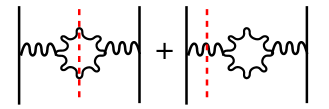
Figure 4: Gluon pair production diagram and the corresponding virtual diagram (vacuum polarization).

This is a diagram with gluon pair production, where the internal singularity occurs when the invariant mass of the produced pair goes to zero. The additional $\epsilon$ pole originating from the singularity $1/k^{2}=1/(k_{1}+k_{2})^{2}$, together with $(\alpha_{1}\alpha_{2})^{2\epsilon}$ factor, will lead to a familiar mixing terms in the residue. This mixing terms leads to the differences between real parton integrals once the different choices of the upper phase space enclosure are applied. Of course, in CFP scheme there is a mechanism which brings back the independence of the inclusive kernels on that. In this case the contributions of the corresponding divergent virtual diagram do this job.

In this case the calculations are technically more complicated and have to remain beyond the scope of this contribution. In fact the independence was explicitly checked by means of switching from the angular scale to the overall virtuality as the upper phase space limiting variable as they are best suited for the singularity structure of these diagrams.

5 Conclusions

We investigate the mechanism which ensures the independence of the NLO DGLAP evolution kernels calculated within Curci-Furmanski-Petronzio scheme on the choice of the upper phase space limiting variable $s(k_{1},k_{2})$.

It was shown that for different groups of Feynman diagrams there are three mechanisms which work in order to compensate the differences due to change of the type of $s(k_{1},k_{2})$. The independence is demonstrated explicitly in case of transverse momentum and rapidity related variable $a$. (The investigation has been carried out also for different choices like overall virtuality $q^{2}$, maximum light-cone variable $k$-minus, but no details are reported here.)

We have show that the mechanisms protecting this property involves either soft counterterms of CFP scheme or virtual diagrams.

In case of the MC implementation of the exclusive PDFs, see refs. [6, 7, 10], keeping track of these phenomena in the kernel calculations is useful for understanding what happens while switching from one version of the evolution time variable in the Monte Carlo to the other, more details will be provided in ref. [11].

Acknowledgments
We would like to acknowledge support and warm hospitality of CERN EP/TH (S.J. and M.S.), University of Manchester (A.K.) and IPPP Durham (M.S.) during the preparation of this work.

References

-
[1]
L.N. Lipatov, Sov. J. Nucl. Phys. 20 (1975) 95;
V.N. Gribov and L.N. Lipatov, Sov. J. Nucl. Phys. 15 (1972) 438;
G. Altarelli and G. Parisi, Nucl. Phys. 126 (1977) 298;
Yu. L. Dokshitzer, Sov. Phys. JETP 46 (1977) 64. - [2] G. Curci, W. Furmanski, and R. Petronzio, Nucl. Phys. B175 (1980) 27.
- [3] R. K. Ellis, H. Georgi, M. Machacek, H. D. Politzer, and G. G. Ross, Phys. Lett. B78 (1978) 281.
- [4] J. C. Collins, D. E. Soper, and G. Sterman, Nucl. Phys. B250 (1985) 199.
- [5] G. T. Bodwin, Phys. Rev. D31 (1985) 2616.
- [6] S. Jadach and M. Skrzypek, Acta Phys. Polon. B40 (2009) 2071–2096, 0905.1399.
- [7] S. Jadach, M. Skrzypek, A. Kusina, and M. Slawinska, 1002.0010.
- [8] F. Hautmann, Acta Phys. Polon. B40 (2009) 2139–2163.
- [9] M. Slawinska and A. Kusina, Acta Phys. Polon. B40 (2009) 2097–2108, 0905.1403.
- [10] M. Skrzypek and S. Jadach, 0909.5588.
- [11] S. Jadach, M. Skrzypek, A. Kusina, and M. Slawinska, Report IFJPAN-IV-2009-6, in preparation.