Higher-order QCD perturbation theory in different schemes: From FOPT to CIPT to FAPT

Abstract

Results on the resummation of non-power-series expansions of the Adler function of a scalar, $D_{S}$, and a vector, $D_{V}$, correlator are presented within fractional analytic perturbation theory (FAPT). The first observable can be used to determine the decay width $\Gamma_{H\to b\bar{b}}$ of a scalar Higgs boson to a bottom-antibottom pair, while the second one is relevant for the $e^{+}e^{-}$ annihilation cross section. The obtained estimates are compared with those from fixed-order (FOPT) and contour-improved perturbation theory (CIPT), working out the differences. We prove that although FAPT and CIPT are conceptually different, they yield identical results. The convergence properties of these expansions are discussed and predictions are extracted for the resummed series of $R_{S}$ and $D_{V}$ using one- and two-loop coupling running, and making use of appropriate generating functions for the coefficients of the perturbative series.

I Introduction

Since the original work of Shirkov and Solovtsov SS97 appeared in 1997, the analytic approach to QCD perturbation theory has evolved and progressed considerably. At the heart of this approach is the spectral density which provides the means to define an analytic running coupling in the Euclidean space via a dispersion relation in accordance with causality and renormalization-group (RG) invariance. Using the same spectral density one can also define the running coupling in Minkowski space by employing the dispersion relation for the Adler function Rad82 ; KP82 ; MS96 ; MiSol97 . In parallel, this approach has been extended beyond the one-loop level MiSol97 ; SS98 and analytic and numerical tools for its application have been developed Mag99 ; Mag00 ; KM01 ; Mag03u ; KM03 ; Mag05 . These efforts culminated in a systematic calculational framework, termed Analytic Perturbation Theory (APT), recently reviewed in SS06 .

The simple analytization of the running coupling and its integer powers has been generalized to the level of hadronic amplitudes KS01 ; Ste02 as a whole and new techniques have been developed to deal with more than one (large) momentum scale SSK99 ; SSK00 ; BPSS04 (for a brief exposition, see Ste04 ). This encompassing version of analytization includes all terms that may contribute to the spectral density, i.e., affect the discontinuity across the cut along the negative real axis $-\infty<Q^{2}<0$. It turns out that logarithms of the second large scale, which can be the factorization scale in higher-order perturbative calculations or the evolution scale, correspond to non-integer indices of the analytic couplings, giving rise—in Euclidean space—to Fractional Analytic Perturbation Theory (FAPT) BMS05 ; BKS05 . This concept was successfully extended to the timelike region and a unified description in the whole complex momentum space was achieved BMS06 (see also SK08 ; Ste09 ). The issue of crossing heavy-flavor thresholds, naturally entering such calculations, has been considered within APT Shi00 ; Shi01 ; SS06 ; BPSS04 and more recently also within FAPT AB08gfapt .

Another important topic, which is at the core of the present investigation, deals with the perturbative summation in (F)APT. As it has been demonstrated in MS04 ; BM08 ; CvVa06 , it is possible to determine the total sum of the perturbative expansion at the level of the one-loop running of the coupling. This result will be extended here to include in the sum at least the two-loop running of the coupling. Even more, making a natural assumption concerning the asymptotic behavior of the perturbative coefficients, proposed long ago by Lipatov Lip76 , we will show that it is possible to estimate the sum of the series to all orders of the expansion. This important feature of the (F)APT non-power series gives us the possibility to estimate the uncertainties of the perturbative results with higher accuracy relative to the conventional QCD power-series expansion. In the present investigation we will extend and systematize these issues towards a complete calculational scheme considering also some applications—including updated predictions for the decay width of a Higgs boson to a bottom–antibottom pair, relevant for the Higgs-boson search at the Tevatron and the LHC.

The paper is organized as follows. In Sec. II we compare the results obtained in different schemes—FOPT, CIPT, and FAPT—and prove that CIPT and FAPT provide identical results for $R_{e^{+}e^{-}\to\text{hadrons}}$ and $R_{\text{S}}$. In addition, we recall in this section the pivotal ingredients of the analytic perturbative approach and discuss briefly its extension to the case of a variable flavor number (the so-called “global case” Shi00 ). Moreover, in Sec. III we describe how typical series expansions within FAPT can be resummed at the level of the one-loop coupling running having recourse to a generating function—referring the reader for the two-loop case to Appendix D. Section IV is devoted to the Higgs-boson decay into a $\bar{b}b$ pair, a process which contains and exhibits the conceptual and technical details of our analytic framework. In the same section, we calculate the associated decay width, which involves the Adler function of a scalar correlator, and compare it with the results of the standard perturbative scheme. Then, in Sec. V, we turn to another application of the proposed resummation technique and consider the Adler function of a vector correlator, pertaining to $R_{e^{+}e^{-}\to\mbox{\footnotesize hadrons}}$. Finally, Sec. VI contains our concluding remarks, while some important technical derivations are given in five Appendices.

II FOPT, CIPT and FAPT

II.1 Two-point correlator of scalar/vector currents

As mentioned in the Introduction, the initial motivation to invent new QCD couplings was the desire to interrelate the Adler $D$-function,

$$D(Q^{2},\mu^{2})\stackrel{{\scriptstyle\mu^{2}=Q^{2}}}{{\longrightarrow}}D(Q^{2})=d_{0}+\sum_{m=1}d_{m}~{}a_{s}^{m}(Q^{2})\,,$$ (1)

calculable in the Euclidean domain, and the quantity $\displaystyle R_{e^{+}e^{-}}=\frac{\sigma(e^{+}e^{-}\to\mbox{hadrons})}{\sigma(e^{+}e^{-}\to\mu^{+}\mu^{-})}$,

$$R(s,\mu^{2})\stackrel{{\scriptstyle\mu^{2}=s}}{{\longrightarrow}}R(s)=r_{0}+\sum_{m=1}~{}r_{m}~{}a_{s}^{m}(s)\,,$$ (2)

which is measured in the Minkowski region. Both quantities are considered in standard QCD perturbation theory, demanding that the couplings entering them satisfy the renormalization-group equation. To facilitate direct comparison of our results further below with the higher-order calculations in standard perturbation theory, in particular Refs. BCK05 ; BCK08 ; BCK10 , we use here the variable $a_{s}\equiv\alpha_{s}/\pi$. Thus, the beta-function coefficients of this coupling are defined by

$$\beta_{s}(a_{s})=\frac{d\,a_{s}(\mu^{2})}{d\ln(\mu^{2})}=-a_{s}\left(\beta_{0}\ a_{s}+\beta_{1}\,a_{s}^{2}+\ldots\right)=-\frac{\alpha_{s}}{\pi}\left[b_{0}\,\left(\frac{\alpha_{s}}{4\,\pi}\right)+b_{1}\,\left(\frac{\alpha_{s}}{4\,\pi}\right)^{2}+\ldots\right]\,,$$ (3)

where $\beta_{n}=b_{n}/4^{n+1}$ and the coefficients $b_{n}$ are specified in Appendix D.

The functions $D$ and $R$ can be related to each other via the following dispersion relations without any reference to perturbation theory

$$R(s)=\hat{R}\left[D\right]\equiv\frac{1}{2\pi\textit{i}}\int_{-s-i\varepsilon}^{-s+i\varepsilon}\!\frac{D(\sigma)}{\sigma}\,d\sigma\,,~{}~{}~{}~{}~{}\\ D(Q^{2})=\hat{D}\left[R\right]\equiv Q^{2}~{}\int_{0}^{\infty}\frac{R(\sigma)}{(\sigma+Q^{2})^{2}}d\sigma~{},$$ (4)

where for the first term in Eq. (4), the integration contour $\Gamma_{1}$ around the cut (solid red line) is shown in Fig. 1. However, employing a perturbative expansion on the LHS of Eqs. (1) and (2), one obtains, in fact, a relation between the powers of $\ln(s/\mu^{2})$ and $\ln(Q^{2}/\mu^{2})$ in the coefficients $r_{m}(s,\mu^{2})$ and $d_{n}(Q^{2},\mu^{2})$, while the powers of the couplings $a_{s}(\mu^{2})$ reveal themselves as parameters.

II.2 Fixed-order perturbation theory

Table 1: This table exemplifies the structure of the first few coefficients $r_{m}=T^{mk}d_{k}$ (summation over $k=1,\ldots,m$ implied) of the conventional expansion of the $R$-ratio, where $T^{mk}$ are the table entries. Each coefficient $r_{m}$ contains a number of $d_{k}~{}(k\leq m)$ terms in its expansion that are shown in the corresponding row. The various contributions are marked by different colors according to their loop order: one-loop—black; two-loop—red; three-loop—blue.

	$\bm{d_{1}}$	$\bm{d_{2}}\vphantom{{}^{\Big{|}}}$	$\bm{d_{3}}$	$\bm{d_{4}}$	$\bm{d_{5}}$
$\bm{r_{1}}\vphantom{{}^{\Big{|}}}$	$\bm{1}$
$\bm{r_{2}}\vphantom{{}^{\Big{|}}}$	$0$	$\bm{1}$
$\bm{r_{3}}\vphantom{{}^{\Big{|}}}$	$\displaystyle-\frac{(\pi\,\beta_{0}\vphantom{{}^{\big{|}}})^{2}}{3}\vphantom{{}^{\big{|}}_{\big{|}}}$	$0$	$\bm{1}$
$\bm{r_{4}}\vphantom{{}^{\Big{|}}}$	$0$ $\displaystyle\bm{-\frac{5\,\pi^{2}\vphantom{{}^{\big{|}}}}{6}\,\beta_{0}\,\beta_{1}}\vphantom{{}^{\big{|}}_{\big{|}}}$	$\displaystyle-\frac{(\pi\beta_{0}\vphantom{{}^{\big{|}}})^{2}}{3}~{}3\vphantom{{}^{\big{|}}_{\big{|}}}$	0	$\bm{1}$
$\bm{r_{5}}\vphantom{{}^{\Big{|}}}$	$\displaystyle\frac{(\pi\,\beta_{0}\vphantom{{}^{\big{|}}})^{4}}{5}\vphantom{{}^{\big{|}}}$  $\displaystyle-\frac{\pi^{2}}{2}\,\beta_{1}^{2}$ $\displaystyle\bm{-\pi^{2}\,\beta_{0}\,\beta_{2}}\vphantom{{}^{\big{|}}_{\big{|}}}$	$\displaystyle 0\vphantom{\frac{(\pi\,\beta_{0}^{\big{|}})^{4}}{5}_{\big{|}}}$ $\displaystyle\bm{-\frac{7\,\pi^{2}}{3}\,\beta_{0}\,\beta_{1}}\vphantom{{}^{\big{|}}}$	$\displaystyle-\frac{(\pi\beta_{0})^{2}}{3}\,6$	0	$\bm{1}$

For the fixed order-$n$ perturbation theory (abbreviated as FOPT), one can start from Eq. (4) and use (2) on its LHS and (1) on its RHS to obtain

$$R^{\text{FOPT}}_{n}(s)\equiv R_{n}(s,\mu^{2}=s)=\frac{1}{2\pi\textit{i}}\int_{-s-i\varepsilon}^{-s+i\varepsilon}\!\frac{D_{n}(\sigma,\mu^{2})}{\sigma}\,d\sigma~{}\Bigg{|}_{\mu^{2}=s}=r_{0}+\sum_{m=1}^{n}r_{m}\left(a_{s}(s)\right)^{m}\,.$$ (5)

To further utilize the FOPT approach, it is useful to consider the relation between the coefficients $r_{m}$ and $d_{k}$ in more detail. The goal is to express the coefficients $r_{m}$ in (5) in terms of the calculable coefficients $d_{n}$ in Eq. (1), i.e., to write $r_{m}=T^{mk}d_{k}$, where summation over $k=1,\ldots,m$ is implied. The matrix $T^{mk}$ is triangular with unity elements on its diagonal—see Table II.2. In the horizontal direction, i.e., along the rows of this Table, we include all coefficients $d_{i}$ up to the coefficient $d_{5}$, the latter not calculated yet, but due to be estimated within our approach later in connection with specific applications—Secs. IV and V).

The elements, proportional to $\beta_{0}^{m}$, which originate from the one-loop evolution procedure, have the following general form

$$d_{n}\,\frac{a_{s}^{n}}{4^{n}}\sum_{m=0}\frac{(n-1+2m)!}{(n-1)!~{}(2m)!}(-1)^{m}\frac{(a_{s}\,\pi\,\beta_{0})^{2m}}{2m+1}$$ (6)

and can be obtained for any fixed order $n$ of the expansion by the procedure described in Appendix A. The other $\beta_{i}$-coefficients—related to higher loops—have been color-printed below using the same color assignments as in Table II.2.

To get acquaintance with the use of this Table, we write out explicitly the relation between $r_{6}$ and $d_{i}$, $i=1,\ldots,6$, (printing the four-loop-order contribution in green color):

$$r_{6} \!\!\!\!=~{}\left[\bm{\frac{(\pi\,\beta_{0})^{2}}{3}\,0}+{\color[rgb]{1,0,0}\bm{\frac{77\,\pi^{4}}{60}\,\beta_{0}^{3}\,\beta_{1}}}-{\color[rgb]{0,0,1}\bm{\frac{7\,\pi^{2}}{6}\,\beta_{1}\,\beta_{2}}}-{\DarkGreen\bm{\frac{7\,\pi^{2}}{6}\,\beta_{0}\,\beta_{3}}}\right]\,d_{1}$$ (7)

$$+\left[\bm{\frac{(\pi\,\beta_{0})^{4}}{5}\,5}-{\color[rgb]{1,0,0}\bm{\frac{4\,\pi^{2}}{3}\,\beta_{1}^{2}}}-{\color[rgb]{0,0,1}\bm{\frac{8\,\pi^{2}}{3}\,\beta_{0}\,\beta_{2}}}\right]\,d_{2}$$

$$+\left[\bm{\frac{(\pi\,\beta_{0})^{2}}{3}\,0}-{\color[rgb]{1,0,0}\bm{\frac{9\,\pi^{2}}{2}\,\beta_{0}\,\beta_{1}}}\right]\,d_{3}$$

$$-\left[\bm{\frac{(\pi\,\beta_{0})^{2}}{3}\,10}\right]\,d_{4}+\left[\bm{\frac{(\pi\,\beta_{0})^{2}}{3}\,0}\right]\,d_{5}+d_{6}\,.$$

The role of the “kinematical $\pi^{2}$”-terms becomes more pronounced for higher orders $m$. For instance, as regards the term $r_{3}$, the underlined $\pi^{2}$-contributions are comparable in size with the original $d_{3}$-contribution, while for $r_{4}$ these contributions even exceed in magnitude the value of the coefficient $d_{4}$ BCK08 ; BCK10 , as one observes from the expressions

$$r_{3} = 18.2-\underline{24.9}+(-4.22+\underline{3.02})n_{f}+(-0.086+\underline{0.091})n_{f}^{2}\,,$$ (8)

$$r_{4} = 135.8-\underline{292.4}+(-34.4+\underline{53.2})n_{f}+(1.88-\underline{2.67})n_{f}^{2}+(-0.01+\underline{0.032})n_{f}^{3}\,.$$ (9)

Therefore, we may be tempted to take into account the “kinematical” $\pi^{2}$-terms to all orders of the expansion, i.e., to sum, for a fixed element $d_{n}$, over the index $m$ along a single column in Table II.2 by taking into account the corresponding power of the coupling $a_{s}^{m}$.

Let us now look at alternative QCD perturbative expansions.

II.3 Contour-improved perturbation theory

Another way to determine $R$ was suggested in Piv91eng ; LeDiPi92 , where the integration contour in Eq. (4) was changed from the cut $\Gamma_{1}$ to the contour $\Gamma_{2}$, i.e., to the circle in the complex $Q^{2}$-plane with radius $s$ centered at $0$, see Fig. 1. Applying the FOPT expansion, the integration of the terms $d_{n}(\sigma/\mu^{2})\,a_{s}^{n}(\mu^{2})$ in Eq. (1), along the contour $\Gamma_{2}$, is completely equivalent to the integration along the cut. Using instead the so-called Contour-Improved Perturbation Theory (CIPT), for large enough values of $s$, one can integrate the terms $d_{n}\,a_{s}^{n}(\sigma)$, entering its RHS, along the contour $\Gamma_{2}$ to get

$$A_{n}\equiv\frac{1}{2\pi i}\int_{\Gamma_{2}}a_{s}^{n}(\sigma)\frac{d\sigma}{\sigma}\,.$$ (10)

This means that one may absorb all logarithms inside the running coupling just by adjusting in Eq. (4) the magnitude of the scale $\mu^{2}=\sigma$—without performing any expansion. CIPT is currently considered to be the most preferable technique to account for the running of perturbative quantities in a number of processes, including the $\tau$-decay GKP01 ; DDGHMZ08 , the $R_{e^{+}e^{-}}$-ratio BCK08 ; BCK10 , and the width of the Higgs-boson decay H$\to b\bar{b}$ KK09 . The integration of the running couplings along the contour $\Gamma_{2}$ is performed numerically DDGHMZ08 , but for the one-loop running the result for $R^{\text{CIPT}}$ can be obtained also analytically and is found to coincide with expression (6), as expected (see Appendix A).

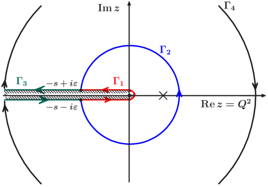
Figure 1: Integration contour $\Gamma_{1}$ entering the calculation of $R(s)$ in Eq. (4). The position of the Landau pole is marked by the cross symbol $\bm{\times}$. The other integration contours shown are explained in the text.

II.4 Fractional analytic perturbation theory

Inspection of Table II.2 suggests to consider the sum of the elements of each of its columns as defining a new coupling. For instance, the first column, associated with $d_{1}$, gives rise to the coupling ${\mathfrak{A}}_{1}$, while the second column pertains to the coupling ${\mathfrak{A}}_{2}$, and so on. In this way, one becomes able to introduce a non-power-series expansion in Minkowski space. This is, actually, just another way to define the Analytic Perturbation Theory SS97 ; MS96 ; SS06 , and its extension—Fractional Analytic Perturbation Theory BMS05 ; BMS06 (see also BKS05 ; KS01 and AB08gfapt ; Ste09 for reviews). The basis of (F)APT is provided by the following linear operations which define analytic images of the normalized coupling $a=a_{s}\,b_{0}/4$ and its powers in the Euclidean and the Minkowski space, respectively:

$${\mathcal{A}}_{\nu}(Q^{2})=\textbf{A}_{\text{E}}\left[a^{\nu}\right]\equiv\int_{0}^{\infty}\!\frac{\rho_{\nu}(\sigma)}{\sigma+Q^{2}}\,d\sigma\,,~{}~{}~{}~{}~{}{\mathfrak{A}}_{\nu}(s)=\textbf{A}_{\text{M}}\left[a^{\nu}\right]\equiv\int_{s}^{\infty}\!\frac{\rho_{\nu}(\sigma)}{\sigma}\,d\sigma~{},$$ (11)

where $\displaystyle\rho_{\nu}(\sigma)=\frac{1}{\pi}\textbf{Im}\,\left[a^{\nu}(-\sigma)\right]$ is the spectral density. The set of the couplings $\{{\mathcal{A}}_{\nu},\ {\mathfrak{A}}_{\nu}\}$ satisfy the dispersion relations Eq. (4) and fulfill the constraint $\hat{R}\hat{D}=\hbox{{1}\kern-2.5pt\hbox{l}}$. Applying the operation $\textbf{A}_{\text{M}}$ on the RHS of the last expression in Eq. (1), one obtains $R$ in APT:

$$\textbf{A}_{\text{M}}[D]=R^{\text{APT}}=d_{0}+\sum_{m=1}\hat{d}_{m}{\mathfrak{A}}_{m}\,.$$ (12)

The reader should note here that the expansion coefficients $d_{n}$ differ from those in Eq. (1) and are defined as follows

$$\hat{d}_{n} = \left(\frac{4}{b_{0}}\right)^{n}d_{n}\,.$$ (13)

The prefactors $(4/b_{0})^{n}$ above—and analogously in Eq. (14) below— serve to connect this analysis to our standard definitions of the analytic couplings $\mathcal{A}_{\nu}$ and $\mathfrak{A}_{\nu}$ in Refs. BMS05 ; BMS06 . Hence, according to Eqs. (11)–(12), one may associate the evaluation of $R$ within (F)APT with the integration contour $\Gamma_{3}$ in Fig. 1.

Consider now how the (F)APT result $R^{\text{APT}}$ in Eq. (12) correlates with the elements of Table II.2. One appreciates that every term $\hat{d}_{m}\,{\mathfrak{A}}_{m}$ of the series appears as an infinite sum of the elements along the corresponding matrix column in this table. The series is convergent and includes all so-called “kinematical terms”, as we discussed at length in BMS06 . One can verify this by considering the expansion of the first few elements $\hat{d}_{m}\,{\mathfrak{A}}_{m}$ in Eq. (14) and then compare the results with the content of the corresponding column in Table II.2. A further advantage of Eq. (14) is that one can use it to derive expression (6) in a more direct way, namely, as an expansion of the one-loop Minkowski analytic couplings ${\mathfrak{A}}_{n}$ in powers of the variable $a_{s}$—terms printed in black color in Eq. (14). The analogous terms for higher loops can be found in Appendix C of Ref. BMS06 . Thus, we obtain (with the same coloring assignments as in Sec. II.2)

$$\left(\frac{4}{b_{0}}\right)^{1}{\mathfrak{A}}^{(3)}_{1}=\!\! \!\!\!\!a_{s}\left[1-\frac{(a_{s}\pi\beta_{0})^{2}}{3}+\frac{(a_{s}\pi\beta_{0})^{4}}{5}+\ldots\right]$$ (14a)

$$\!{\color[rgb]{1,0,0}\bm{-}}\! \!\!{\color[rgb]{1,0,0}\bm{\frac{\pi^{2}}{3}\,a_{s}^{4}\,\Big{(}\beta_{0}\beta_{1}\frac{5}{2}+\beta_{1}^{2}\frac{3}{2}a_{s}-\frac{\pi^{2}}{5}\beta_{0}^{3}\beta_{1}\frac{77}{4}a_{s}^{2}+\ldots\Big{)}}}$$

$$\!{\color[rgb]{0,0,1}\bm{-}}\! \!\!{\color[rgb]{0,0,1}\bm{\frac{\pi^{2}}{3}\,a_{s}^{5}\,\left(\beta_{0}\beta_{2}~{}3+\beta_{1}\beta_{2}~{}\frac{7}{2}a_{s}+\ldots\right)}}$$

$$\!{\DarkGreen\bm{-}}\! \!\!{\DarkGreen\bm{\frac{\pi^{2}}{6}\,a_{s}^{6}\,\beta_{0}\beta_{3}\,7}}+\ldots$$

$$\left(\frac{4}{b_{0}}\right)^{2}{\mathfrak{A}}^{(2)}_{2}=\!\! \!\!\!\!a^{2}_{s}\left[1-(a_{s}\pi\beta_{0})^{2}+(a_{s}\pi\beta_{0})^{4}~{}\ldots\right]$$ (14b)

$$\!{\color[rgb]{1,0,0}\bm{-}}\! \!\!{\color[rgb]{1,0,0}\bm{\frac{\pi^{2}}{3}\,a^{5}_{s}\,\left(\beta_{0}\beta_{1}7+\beta_{1}^{2}4a_{s}+\ldots\right)}}$$

$$\!{\color[rgb]{0,0,1}\bm{-}}\! \!\!{\color[rgb]{0,0,1}\bm{\frac{\pi^{2}}{3}\,a_{s}^{6}\,\beta_{0}\,\beta_{2}\,8}}+\ldots$$

$$\left(\frac{4}{b_{0}}\right)^{3}{\mathfrak{A}}^{(2)}_{3}=\!\! \!\!\!\!a^{3}_{s}\left[1-\frac{(a_{s}\pi\beta_{0})^{2}}{3}6~{}+\ldots\right]$$ (14c)

$$\!{\color[rgb]{1,0,0}\bm{-}}\! \!\!{\color[rgb]{1,0,0}\bm{\frac{\pi^{2}}{3}\,a_{s}^{6}\,\beta_{0}\beta_{1}\frac{27}{2}}}+\ldots$$

$$\left(\frac{4}{b_{0}}\right)^{4}{\mathfrak{A}}^{(2)}_{4}=a^{4}_{s}\left[1-\frac{(a^{2}_{s}\pi\beta_{0})^{2}}{3}10+\ldots\right]+\ldots$$ (14d)

The main conclusion from the above exposition is that, depending on the particular scheme of the perturbative expansion used, the elements of Table II.2 may be summed in different ways (see Table 2). Specifically,

1. FOPT gives the sum of a finite number of terms along some row to create $r_{m}$, and then—following Eq. (5)—it sums the results up to $n$ to yield $R_{n}$, i.e., $R_{n}=d_{0}+\sum\limits^{n}_{m,k=1}a_{s}^{m}\,T^{mk}\,d_{k}$.

2. (F)APT takes into account each infinite column as a whole in the form of the expansion $\hat{d}_{m}\,{\mathfrak{A}}_{m}$, thus including this way all “kinematical terms” by construction, and then sums a number of ${\mathfrak{A}}_{m}$ terms into $R^{\text{APT}}_{n}$ in the form given by expression (12).

It is evident that for any fixed order $n$, the results for $R_{n}$ and $R^{\text{APT}}_{n}$ cannot coincide. Nevertheless, it was shown in BMS06 that calculating the decay width of a Higgs boson into a $b\bar{b}$ pair using CIPT, leads to the same result one would obtain for $R$ using FAPT with one-loop running of the coupling. This coincidence turns out to be not accidental but to hold at any loop order of the perturbative expansion by virtue of the dispersion relation given in Eq. (11), as we will prove next.

Table 2: QCD observable $R$ calculated with different perturbative expansions: (F)APT—(Fractional) Analytic Perturbation Theory; CIPT—Contour-Improved Perturbation Theory; FOPT—Fixed-Order Perturbation Theory. The associated contours $\Gamma_{1}$, $\Gamma_{2}$, $\Gamma_{3}$ are displayed in Fig. 1.

Perturbative scheme	Contours	$R$ expansion
FOPT	$\Gamma_{1}$	$\sum_{n}r_{n}a_{s}^{n}$
CIPT	$\Gamma_{2}$	$\sum_{n}d_{n}A_{n}$
(F)APT	$\Gamma_{3}$	$\sum_{n}\hat{d}_{n}\mathfrak{A}_{n}$

II.5 Fixed flavor number vs. global FAPT

We commence our analysis within FAPT by recalling the salient features of the analytic approach to QCD perturbation theory, expanding our remarks given in Section II.4. In order to have a direct connection to our previous papers on the subject BMS05 ; BKS05 ; BMS06 , and to simplify the main formulae in those sections where we consider fixed-order (F)APT with a constant value of active flavors $N_{f}$, we use here the normalized coupling of perturbative QCD (pQCD) MS04 $a=\beta_{f}\,\alpha_{\text{s}}$ with the useful abbreviation $\beta_{f}\equiv b_{0}(N_{f})/(4\,\pi)=(11-2\,N_{f}/3)/(4\,\pi)$, where $b_{0}(N_{f})$ denotes the first coefficient of the QCD $\beta$ function. Analytic images of the normalized coupling and its powers are constructed by means of the linear operations $\textbf{A}_{\text{E}}$ and $\textbf{A}_{\text{M}}$ according to (11) using the spectral density $\displaystyle\rho_{\nu}(\sigma)=\frac{1}{\pi}\textbf{Im}\,\left[a^{\nu}(-\sigma)\right]$.

To be in line with the above definitions, we also introduce analogous expressions for the fixed-$N_{f}$ quantities with standard normalization, i.e.,

$$\bar{\mathcal{A}}_{\nu}(Q^{2};N_{f})=\frac{{\mathcal{A}}_{\nu}(Q^{2})}{\beta_{f}^{\nu}}\,,\quad\bar{\mathfrak{A}}_{\nu}(s;N_{f})=\frac{{\mathfrak{A}}_{\nu}(s)}{\beta_{f}^{\nu}}\,,$$ (15)

which correspond to the analytic couplings ${\mathcal{A}}_{\nu}$ and ${\mathfrak{A}}_{\nu}$ in the Shirkov–Solovtsov terminology SS06 . These couplings have dispersive representations of the type (11) with spectral densities $\bar{\rho}_{\nu}(\sigma;N_{f})={\rho}_{\nu}(\sigma)/{\beta_{f}^{\nu}}$. For the sake of simplicity we will omit to display $N_{f}$ (and other evident arguments) explicitly. In the present analysis we express all variables in terms of $L=\ln(Q^{2}/\Lambda^{2})$ (Euclidean space) or $L=\ln(s/\Lambda^{2})$ (Minkowski space), using the notation defined above, but with an argument placed in square brackets: $a^{\nu}[L]$, ${\mathcal{A}}_{\nu}[L]$, and ${\mathfrak{A}}_{\nu}[L]$. Then, in the one-loop approximation (labeled by the superscript (1)), we have

$$a^{(1)}[L]=\frac{1}{L}\,,\quad{\mathcal{A}}^{(1)}_{1}[L]=\frac{1}{L}-\frac{1}{e^{L}-1}\,,\quad{\mathfrak{A}}^{(1)}_{1}[L]=\frac{1}{\pi}\,\arccos\left(\frac{L}{\sqrt{L^{2}+\pi^{2}}}\right)\,,$$ (16a)

$$\rho^{(1)}_{1}[L]=\frac{1}{L^{2}+\pi^{2}}\,,\quad\bar{\rho}^{(1)}_{1}[L;N_{f}]=\frac{1}{\beta_{f}\left(L^{2}+\pi^{2}\right)}\,.$$ (16b)

On the other hand, when we will discuss the global version of (F)APT, where $Q^{2}$ (or $s$) varies in the whole (“global”) domain $[0,\infty)$, and $N_{f}$ effectively becomes dependent on $Q^{2}$ (or $s$), we will use in Eq. (11) the global version of the spectral density that takes into account threshold effects and is, therefore, $N_{f}$-dependent.

In order to make the effect of crossing a heavy-quark threshold more plausible, consider a single threshold at $\sigma=m_{4}^{2}$ (corresponding to the transition $N_{f}=3\Rightarrow N_{f}=4$) and write the spectral density in a form which expresses it in terms of the fixed-flavor spectral densities with 3 and 4 flavors, $\bar{\rho}_{n}[L;3]$ and $\bar{\rho}_{n}[L+\lambda_{4};4]$, respectively. The result is

$$\rho_{\nu}^{\text{\tiny glob}}(\sigma)=\rho_{\nu}^{\text{\tiny glob}}[L_{\sigma}]=\theta\left(L_{\sigma}<L_{4}\right)\,\bar{\rho}_{\nu}\left[L_{\sigma};3\right]+\theta\left(L_{4}\leq L_{\sigma}\right)\,\bar{\rho}_{\nu}\left[L_{\sigma}+\lambda_{4};4\right]~{}~{}~{}$$ (17)

with $L_{\sigma}\equiv\ln\left(\sigma/\Lambda_{3}^{2}\right)$, $L_{4}\equiv\ln\left(m_{4}^{2}/\Lambda_{3}^{2}\right)$, and $\lambda_{4}\equiv\ln\left(\Lambda_{3}^{2}/\Lambda_{4}^{2}\right)$. Note, however, that in standard QCD perturbation theory the coupling at the threshold becomes discontinuous. To enable a smooth matching at this point, one has to readjust the values of $\Lambda_{\text{QCD}}$ on each side of the threshold in correspondence with their associated flavor numbers ($\Lambda_{f}=\Lambda_{\text{QCD}}^{N_{f}=f}$).

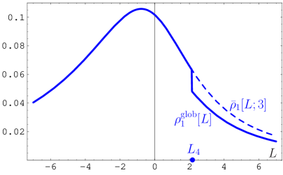
Figure 2: Spectral densities $\rho_{1}^{\text{\tiny glob}}[L]$ (solid line) and $\bar{\rho}_{1}[L;3]$ (dashed line). The discontinuity at $L=L_{4}$ is artificially enhanced by a factor of 1.5 to make it more visible.

In Fig. 2 we show the global spectral density $\rho_{1}^{\text{\tiny glob}}[L]$ in comparison with the spectral density $\bar{\rho}_{1}[L;3]$ which corresponds to a fixed flavor number $N_{f}=3$. We see that, because of the different values of $\Lambda_{3}$ and $\Lambda_{4}$, and also of $\beta_{3}$ and $\beta_{4}$, these quantities differ from each other when $L$ crosses $L_{4}$.

Substituting the obtained spectral density $\rho_{\nu}^{\text{\tiny glob}}(\sigma)$ [cf. Eq. (17)] into Eq. (11), we get continuous expressions for the analytic couplings in both domains of the complex $Q^{2}$ space. In the Minkowski region, the global analytic coupling reads

$${\mathfrak{A}}_{\nu}^{\text{\tiny glob}}[L]=\theta\left(L\!<\!L_{4}\right)\Bigl{\{}\bar{{\mathfrak{A}}}_{\nu}[L;3]-\bar{{\mathfrak{A}}}_{\nu}[L_{4};3]+\bar{{\mathfrak{A}}}_{\nu}[L_{4}+\lambda_{4};4]\Bigr{\}}+\theta\left(L_{4}\!\leq\!L\right)\,\bar{{\mathfrak{A}}}_{\nu}[L+\lambda_{4};4]\,,~{}~{}~{}$$ (18)

whereas its Euclidean counterpart assumes the form (referring for more details to BM08 ; AB08gfapt )

$${\cal A}_{\nu}^{\text{\tiny glob}}[L] = \bar{{\cal A}}_{\nu}[L+\lambda_{4};4]+\int\limits_{-\infty}^{L_{4}}\!\frac{\bar{\rho}_{\nu}[L_{\sigma};3]-\bar{\rho}_{\nu}[L_{\sigma}+\lambda_{4};4]}{1+e^{L-L_{\sigma}}}\,dL_{\sigma}\,.$$ (19)

To demonstrate the magnitude of the threshold corrections, we show in Fig. 3 the values of the normalized deviations $\Delta\overline{\mathcal{A}}_{\nu}[L]={\mathcal{A}}_{\nu}^{\text{\tiny glob}}[L]-\overline{\mathcal{A}}_{\nu}[L\!+\!\lambda_{4};4]$ and $\Delta\overline{\mathfrak{A}}_{\nu}[L]={\mathfrak{A}}_{\nu}^{\text{\tiny glob}}[L]-\overline{\mathfrak{A}}_{\nu}[L\!+\!\lambda_{4};4]$ in the Euclidean and the Minkowski domain, respectively.

   

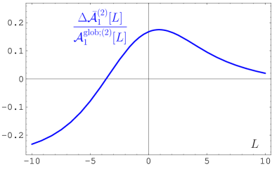
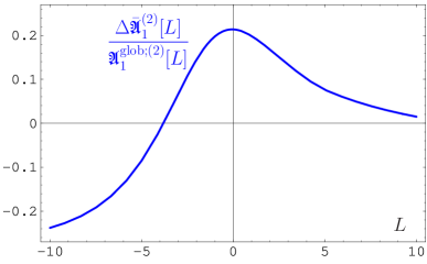
Figure 3: Left: Deviation of the global coupling relative to the fixed-$N_{f}$ coupling in FAPT: $\Delta\overline{\mathcal{A}}_{1}[L]/\mathcal{A}_{1}^{\text{\tiny glob}}[L]$. Right: The same for $\Delta\overline{\mathfrak{A}}_{1}[L]/\mathfrak{A}_{1}^{\text{\tiny glob}}[L]$.

We see that in both domains these deviations vary from $-20\%$ for large values of $-L\approx 10$, going through zero in the vicinity of $L\approx-5$, and then increase up to the value $+20\%$ for $L\approx 0$, tending, finally, to 0 as $L\to\infty$. This means that these deviations reach the level of 10% in the region of several tens of GeV².

II.6 Relation between CIPT and (F)APT

To establish the equivalence between FAPT and CIPT, we consider a more general expansion than Eq. (1) which contains the coupling with a non-integer power that can be related to an anomalous dimension. Such a quantity reads

$$D_{\nu}=d_{0}a_{s}^{\nu}+\sum_{n=1}d_{n}a_{s}^{\nu+n}\,,$$ (20)

where $\nu$ is not an integer number.

Symbolically, we have the following equivalence

$$\text{FAPT}\left(\int_{\Gamma_{3}}\right)=\text{CIPT}\left(\int_{\Gamma_{2}}\right)\,,$$ (21)

referring for the integration contours to Fig. 1. To establish the equivalence between FAPT and CIPT in the above relation, we employ the chain of the equalities

$$\text{FAPT}\equiv\int_{s}^{\infty}\!\frac{\rho_{\nu}(\sigma)}{\sigma}\,d\sigma\equiv\int_{s}^{\infty}\!\frac{\textbf{Im}\,\left[a^{\nu}(-\sigma)\right]}{\pi}\frac{d\sigma}{\sigma}\ =-\frac{1}{2\pi i}\int_{\Gamma_{3}}a^{\nu}(\sigma)\frac{d\sigma}{\sigma}\,,$$ (22)

where in the last step the integral has to be evaluated along the contour $\Gamma_{3}$. On the other hand, the CIPT part of Eq. (21) can be identically rewritten as

$$\text{CIPT}\equiv\frac{1}{2\pi i}\int_{\Gamma_{2}}a^{\nu}(\sigma)\frac{d\sigma}{\sigma}\,.$$ (23)

Therefore, we have to prove that

$$\int_{\Gamma_{3}}\left(a(\sigma)\right)^{\nu}\frac{d\sigma}{\sigma}+\int_{\Gamma_{2}}\left(a(\sigma)\right)^{\nu}\frac{d\sigma}{\sigma}=0\,.$$ (24)

To this end, we close the contour $\Gamma_{3}$ along the large circle $\Gamma_{4}$ with radius $R$ that tends to $\infty$, and take into account the closed composed contour $\Gamma_{234}=\Gamma_{2}\cup\Gamma_{3}\cup\Gamma_{4}$ (see Fig. 1). The integral $I(\Gamma_{234})$,

$$I(\Gamma_{234})=\frac{1}{2\pi i}\oint_{\Gamma_{234}}a^{\nu}(\sigma)\frac{d\sigma}{\sigma}\,,$$ (25)

along the closed contour $\Gamma_{234}$ is equal to the sum of the residues inside the enclosed region. Provided the radius $s$ of the contour $\Gamma_{2}$ is large enough, no poles from $a(\sigma)$ owing to perturbation theory are inside the contour $\Gamma_{234}$. As a result, $I(\Gamma_{234})=0$. Moreover, $(a(\sigma))^{\nu}$ ($\nu>0$) on the contour $\Gamma_{4}$ decreases with growing $R$, and therefore this contribution vanishes as $R\to\infty$. Consequently, we finally obtain

$$I(\Gamma_{234})\stackrel{{\scriptstyle R\to\infty}}{{\longrightarrow}}I(\Gamma_{2}\cup\Gamma_{3})=\frac{1}{2\pi i}\int_{\Gamma_{2}\cup\Gamma_{3}}a^{\nu}(\sigma)\frac{d\sigma}{\sigma}=0\,.$$ (26)

The above equivalence not withstanding, there is a crucial advantage of the FAPT approach with respect to CIPT. In fact, as long as one is only interested in a numerical estimate, CIPT provides acceptable results for several typical processes. However, if one pretends to employ analytic expressions, and thereby to control each step of the calculation, CIPT is not sufficient. In that case, one needs another perturbative scheme that is able to yield explicit expressions for the couplings along each column in Table II.2. Such a scheme is naturally provided by (F)APT. Moreover, we shall show below that this scheme can even admit the resummation over columns BM08 . This is an important feature, given that the conventional perturbative series in Eq. (1) cannot amount to a unique, i.e., resummation-method-independent, result owing to the asymptotic nature of the power series.

III Resummation in (F)APT in the one-loop order

In this section, we consider different sorts of perturbation-series expansions of typical physical quantities, like the Adler function, $D[L]$. Our goal is to perform the summation of such expansions under the imposition of a couple of basic constraints. As we will show in a moment, these constraints are (i) a recurrence relation for higher-order couplings and (ii) the nonpower character of the series. These considerations will be based on an appropriate generating function for the expansion coefficients.

In what follows we discuss in detail the one-loop running case. However, also the technically more complicated two-loop running case is worked out and the corresponding expressions are provided in Appendix D.

III.1 Generating function for the series expansion

At the one-loop level BMS06 , we have

$$\left\{\begin{array}[]{l}D[L]\\ {D}^{\text{\tiny APT}}[L]\\ {R}^{\text{\tiny APT}}[L]\end{array}\right\}=d_{0}+\hat{d}_{1}\sum_{n=1}^{\infty}\tilde{d}_{n}\,\left\{\begin{array}[]{l}a^{n}[L]\\ {\mathcal{A}}_{n}[L]\\ {\mathfrak{A}}_{n}[L]\end{array}\right\}$$ (33)

with $\tilde{d}_{n}\equiv\hat{d}_{n}/\hat{d}_{1}$ [cf. Eq. (13)], where $L=\ln\left(Q^{2}/\Lambda^{2}\right)$ applies to the Euclidean quantities ($D[L]$, ${D}^{\text{\tiny APT}}[L]$, $a^{n}[L]$, and ${\mathcal{A}}_{n}[L]$), and $L=\ln\left(s/\Lambda^{2}\right)$ pertains to their Minkowski versions ${R}^{\text{\tiny APT}}[L]$ and ${\mathfrak{A}}_{n}[L]$.

The resummation of this series is on the focus of the present work. For this purpose, it is useful to introduce a generating function $P(t)$ for the series expansion and write

$$\tilde{d}_{n}=\int_{0}^{\infty}\!\!P(t)\,t^{n-1}dt~{}~{}~{}\text{with}~{}~{}~{}\int_{0}^{\infty}\!\!P(t)\,dt=1\,.$$ (34)

We will show in the next step how to use this generating function in order to resum nonpower series expansions (both in the Euclidean and the Minkowski region). But first recall that the standard coupling $a^{n}$ of perturbative QCD, as well as the couplings ${\mathcal{A}}_{n},{\mathfrak{A}}_{n}$—together with the spectral density $\rho_{n}$—satisfy a one-loop renormalization-group equation that can be recast in the form of a recurrence relation Shi98 :

$$\left\{\begin{array}[]{l}a^{n+1}[L]\\ {\mathcal{F}}_{n+1}[L]\\ \end{array}\right\}=\frac{1}{\Gamma(n+1)}\left(-\frac{d}{dL}\right)^{n}\left\{\begin{array}[]{l}a^{1}[L]\\ {\mathcal{F}}_{1}[L]\\ \end{array}\right\}\,.$$ (35)

Here ${\mathcal{F}}[L]$ denotes one of the analytic quantities ${\mathcal{A}}[L],~{}{\mathfrak{A}}[L],~{}\rho[L]$. Substituting Eqs. (34) and (35) into the perturbative-series expansion, i.e., into Eq. (33), one obtains MS04 in analogy to the previous equation,

$$\left\{\begin{array}[]{l}D[L]\\ {\mathcal{S}}[L]\\ \end{array}\right\}=d_{0}+\hat{d}_{1}\sum_{n=0}^{\infty}\frac{\left\langle\!\left\langle{(-t)^{n}}\right\rangle\!\right\rangle_{P}}{n!}\,\frac{d^{n}}{dL^{n}}\left\{\begin{array}[]{l}a[L]\\ {\mathcal{F}}_{1}[L]\\ \end{array}\right\}=d_{0}+\hat{d}_{1}\left\{\begin{array}[]{l}\left\langle\!\left\langle{a[L-t]}\right\rangle\!\right\rangle_{P}\\ \left\langle\!\left\langle{{\mathcal{F}}_{1}[L-t]}\right\rangle\!\right\rangle_{P}\\ \end{array}\right\}\,,~{}~{}~{}$$ (42)

where $\mathcal{S}=D^{\text{\tiny APT}}$ or $R^{\text{\tiny APT}}$—depending on the choice of the analytic couplings $\mathcal{F}=\mathcal{A}$ or $\mathcal{F}=\mathfrak{A}$, respectively. In the above equation, and in the considerations to follow, we use the abbreviated notation

$$\left\langle\!\left\langle{{\mathcal{F}}[L-t]}\right\rangle\!\right\rangle_{P}\equiv\int^{\infty}_{0}{\mathcal{F}}[L-t]P(t)~{}dt\,.$$ (43)

As long as we have not proved that summation and integration can be interchanged, this representation has only a formal meaning. Note, however, that the integration over the Taylor-series expansion of the term $a[L-t]$ in the integrand reproduces the initial series for any partial sum. The integrand in the standard case of the QCD running coupling (first line in Eq. (42)) faces a pole singularity (termed the infrared renormalon singularity) and is, therefore, ill-defined. In contrast, the integral in the second entry in Eq. (42) has a rigorous meaning by virtue of the finiteness of $\mathcal{F}_{1}[L]$, being one of the quantities $\{\mathcal{A}_{1}[L],\ \mathfrak{A}_{1}[L]\leq 1,\ \rho_{1}[L]\leq 1/\pi^{2}\}$. Therefore, the expression on the RHS of Eq. (42), together with (43), can be called the sum of the corresponding series in the sense of Euler. Since any coefficient $\tilde{d}_{n}$ is the moment of $P(t)$ [cf. Eq. (34)], this function should fall off faster than any power—e.g., like an exponential or faster. Therefore, all APT expressions on the RHS of Eq. (42) (second line) exist and are proportional to ${\mathcal{F}}[L-\bar{t}(L)]$, where, for each $L$, $\bar{t}(L)$ is the average value of $t$ associated with this quantity.

Provided the generating function is known, one can compute the integral (43) explicitly and obtain this way all-order estimates for the expanded quantity for any series expansion, provided the coupling parameters fulfill the following conditions: (i) satisfy the one-loop renormalization-group equation [cf. Eq. (35)], (ii) are real, and (iii) have only integrable singularities. If the first coefficient $d_{0}$ of the expansion (33) is not accompanied by unity ($a^{0}$), but by some other fractional power $\nu$ of the coupling ($a^{\nu}$), then, as it has been shown in BM08 ; AB08gfapt , the resummation method (42) has to be modified to read

$$\mathcal{S}_{\nu}[L]=d_{0}\,\mathcal{F}_{\nu}[L]+\hat{d}_{1}\left\langle\!\left\langle{{\mathcal{F}}_{1+\nu}[L-t]}\right\rangle\!\right\rangle_{P_{\nu}}\,,$$ (44)

where now the generating function $P_{\nu}$ depends also on $\nu$. This quantity can be deduced from $P$ as follows:

$$P_{\nu}(t)=\int_{0}^{1}\!P\left(\frac{t}{1-x}\right)\Phi_{\nu}(x)\frac{dx}{1-x}\,.$$ (45)

Here $\Phi_{\nu}(x)=\nu x^{\nu-1}$, so that $\lim_{\nu\to 0}\Phi_{\nu}\rightarrow\delta(x)$, and therefore $\lim_{\nu\to 0}P_{\nu}(t)=P(t)$. The last step completes the generalization of the original APT resummation procedure of MS04 to the case of FAPT.

III.2 Modeling the expansion coefficients and their generating function

For most relevant QCD processes, only the first few coefficients $d_{n}$ are known, while the computation of higher-order coefficients is technically a highly complicated task. This is despite the impressing development of sophisticated algorithms during the last few years BCK02 ; BCK05 ; BCK08 ; BCK10 ; BeJam08 . In view of this, it is extremely useful to have alternative methods for calculating the higher-order coefficients, let alone to resum the whole series—even if the result represents a sort of approximation—provided the quality of the applied method is high and the inherent uncertainties entailed can be kept under control. On the other hand, the asymptotic form of the coefficients $\hat{d}_{n}$ can be predicted from

$$\hat{d}_{n}\sim\Gamma(n+1)~{}n^{\gamma}c^{n}\left[1+O(1/n)\right]\to P(t)\sim(t/c)^{\gamma+1}e^{-t/c}$$ (46)

a form that is inspired by Lipatov’s asymptotic expression in Ref. Lip76 (see also KS80 , and Fisch97 for a review), and where $\gamma<1$ and $c$ are numerical coefficients. One anticipates that the large-order behavior of the expansion coefficients translates into the asymptotic form of the generating function $P(t)$.

To proceed, we have to construct first a model for the expansion coefficients $\tilde{d}_{n}=\hat{d}_{n}/\hat{d}_{1}$, having recourse to the information about the first few fixed-order coefficients. The second step is to interpolate between the obtained result and the expression for the tail obtained for $\hat{d}(n)$ from (46) at asymptotically large orders $n$. For a fixed-sign series we adopt the model (note the normalization $\tilde{d}^{\text{model}}_{1}=1$)

$$\tilde{d}^{\text{model}}_{n} = \frac{A_{1}c^{n}n^{\gamma_{1}}n!+A_{2}c^{n-1}n^{\gamma_{2}}(n-1)!}{A_{1}c+A_{2}}\,,$$ (47)

where the parameters $A_{i}$, $\gamma_{i}$, and $c$ are determined from the values of the first few known coefficients $\hat{d}_{n}$. We mention incidentally that the case of an alternating-sign series has been considered in MS04 and will not be addressed here. As regards the most general case of the series, the behavior of $\tilde{d}^{\text{model}}_{n}$ with respect to $n$ turns out to be the same as what is obtained in the renormalon approach (that is usually supplied with the Naive Non-Abelization (NNA) BroGro95 ), see, e.g., BroadKa93 —except perhaps for the specific values of the parameters which are different. Modeling the expansion coefficients according to Eq. (47), leads to the following generating function $P(t)$:

$$P^{\text{model}}(t) \sim \left[A_{1}(t/c)^{1+\gamma_{1}}+A_{2}(t/c)^{\gamma_{2}}\right]\,e^{-t/c}\,.$$ (48)

Using the first already known coefficients, we can calibrate our model in order to extract information about still higher and unknown orders, as well as to gain information on the resumed behavior of the whole series. It should be emphasized that for large values of the argument $t$, our model for $P(t)$ can become rather crude. This, however, does not significantly change the final result of the summation due to the convergence of the integral in Eq. (43). For this reason, it is not necessary to know the asymptotic behavior of $P^{\text{model}}(t)$ very accurately. All said, let us now consider concrete examples to understand the modus operandi and the benefits of this technology.

IV Master example: Higgs-boson decay into a $\bar{b}b$ pair

Our goal in this section is the calculation of the width of the Higgs-boson decay into a $\bar{b}b$ pair, i.e.,

$$\Gamma_{H\to b\bar{b}}(M_{H})=\Gamma_{0}^{b}(m_{b}^{2})\,\frac{\widetilde{R}_{\text{S}}(M_{H}^{2})}{3\,m_{b}^{2}}\,,$$ (49)

where $\Gamma_{0}^{b}(m_{b}^{2})=3\,G_{F}\,M_{H}\,m_{b}^{2}/{4\sqrt{2}\pi}$, $m_{b}$ and $M_{H}$ are the pole mass of the $b$-quark and the mass of the Higgs boson, respectively, and $\widetilde{R}_{\text{S}}(M_{H}^{2})=\bar{m}^{2}_{b}(M_{H}^{2})\,R_{\text{S}}(M_{H}^{2})$. Our interest in this quantity derives from the fact that this process contains all main ingredients for such high-order calculations, discussed above, with known coefficients up to the order $O(\alpha_{s}^{4})$ BCK05 . The quantity $R_{\text{S}}(s)$ is the discontinuity $R_{\text{S}}(s)=\textbf{Im}\,\Pi(-s-i\epsilon)/{(2\pi\,s)}$ of the imaginary part of the correlator $\Pi$ of the two scalar currents $J^{S}_{b}=\bar{\Psi}_{b}\Psi_{b}$ for bottom quarks with an on-shell mass $m_{b}$ coupled to the scalar Higgs boson with mass $M_{H}$, and it is given by Π(Q^2) = (4π)^2 i∫dx e^iqx⟨0— T[ J^S_b(x) J^S_b(0) ] —0⟩  , where $Q^{2}=-q^{2}$. Direct multi-loop calculations are usually performed in the far Euclidean (spacelike) region for the corresponding Adler function $D_{\text{S}}$ Che96 ; BCK05 ; BKM01 ; KK09 , where QCD perturbation theory works reliably. Hence, we write

$$\frac{Q^{2}}{6}\frac{d}{dQ^{2}}\left(\frac{\Pi(Q^{2})}{Q^{2}}\right)=D_{\text{S}}(Q^{2}) = \left[1+\sum_{n\geq 1}d_{n}\,a_{s}^{n}(Q^{2})\right]\,.$$ (50)

IV.1 Generating function for the scalar correlator and estimates for higher-order coefficients

The Adler function, related to the scalar correlator (see BCK05 ; BMS06 ) and pertaining to the Higgs-boson decay, reads

$$D_{\text{S}}[L] = 1+d_{1}\,\sum_{n=1}^{\infty}\tilde{d}_{n}\,\left(a_{s}[L]\right)^{n}\,.$$ (51)

Note that here the definition of the coefficients $\tilde{d}_{n}$ is given by $\tilde{d}_{n}=d_{n}/d_{1}$. The $n$-dependence of the coefficients $\tilde{d}_{n}$, in accordance with expression (47), can be simulated by the following two-parameter model

$$\tilde{d}_{n}^{H}=c^{n-1}\frac{n+\delta}{1+\delta}\,\Gamma(n)\,,$$ (52a)

a form which ensures that $$\tilde{d}_{1}^{H} H$$ (the superscript denoting “Higgs”) is automatically equal to unity. Concurrently, these coefficients can be reproduced by the following generating function:

$$P_{H}(t)=\frac{(t/c)+\delta}{c\,(1+\delta)}\,e^{-{t/c}}\,.$$ (52b)

To test these formulae, we use the two known coefficients $\tilde{d}_{2}$ and $\tilde{d}_{3}$ for this process and plug them into model (52a) aiming to predict the next two coefficients $\tilde{d}_{4}^{H}$ and $\tilde{d}_{5}^{H}$. The result for the next coefficient $\tilde{d}_{4}^{H}$ is shown in the second row of Table 3: $\tilde{d}_{4}^{H}=662$. We see that it is fairly close to the value 620 calculated recently by Chetyrkin et al. in BCK05 . This procedure can be geared up to predict the next coefficient $\tilde{d}_{5}$. Indeed, taking into account the coefficient $\tilde{d}_{4}$ and slightly readjusting the parameters $c$ and $\delta$ of our model (52b) from their previous values $\left\{c=2.5,~{}\delta=-0.48\right\}$ to $\left\{c=2.4,~{}\delta=-0.52\right\}$, we find (third row in Table 3) $\tilde{d}_{5}\approx 7826$. This result agrees very well with the value $7782$, derived in KaSt95 by appealing to the Principle of Minimal Sensitivity (PMS). Moreover, it has a reasonable agreement with our previous models (rows 3 and 4 in Table 3) and also with the improved NNA (INNA) prediction shown in row 7, while the original NNA prediction (value given in row 6) fails. We may conclude that our model calculation of the coefficient $d_{5}$ is congruent with the prediction following from the application of the PMS method. Both these approaches provide results for most coefficients $d_{n}$ approximately twice larger than those found by applying the INNA approximation.

Table 3: Perturbation Theory (PT) coefficients $\tilde{d}_{n}$ for the $D_{\text{S}}$ series obtained from different calculations.

PT coefficients  $\tilde{d}_{1}\vphantom{{}^{|}_{|}}$  $\tilde{d}_{2}$  $\tilde{d}_{3}$  $\tilde{d}_{4}$  $\tilde{d}_{5}$ 1 pQCD results from BCK05 $1\vphantom{{}^{|}_{|}}$  7.42  62.3  620  — – Models and estimates 2 Model (52) with $c=2.5,~{}\delta=-0.48$ $1\vphantom{{}^{|}_{|}}$  7.42  62.3  662  8615 3 Model (52) with $c=2.4,~{}\delta=-0.52$ $1\vphantom{{}^{|}_{|}}$  7.50  61.1  625  7826 4 “PMS” predictions from ChKS97 ; BCK05 ; KaSt95  $-\vphantom{{}^{|}_{|}}$  $-$  64.8  547  7782 5 “NNA” predictions from BKM01 ; BroadKa02 $1\vphantom{{}^{|}_{|}}$ 3.87  21.7  122  1200 6 “INNA” predictions from App. C $1\vphantom{{}^{|}_{|}}$ 3.87  36  251  4930

IV.2 Higgs-boson decay width in FAPT

Within the one-loop approximation of FAPT, the quantity $\widetilde{R}_{\text{S}}(M_{H}^{2})$ has the following non-power series expansion:

$$\widetilde{R}_{\text{S}}^{\text{\tiny FAPT}}[L]=3\,\hat{m}_{(1)}^{2}\,\left\{{\mathfrak{A}}_{\nu_{0}}^{\text{\t{i}ny glob}}[L]+d_{1}\,\sum_{n\geq 1}\frac{\tilde{d}_{n}}{\pi^{n}}\,{\mathfrak{A}}_{n+\nu_{0}}^{\text{\tiny glob}}[L]\right\}\,.$$ (53)

Here $\hat{m}_{(1)}^{2}$ is the renormalization-group invariant mass satisfying the one-loop $\bar{m}^{2}_{b}(\mu^{2})$ evolution equation

$$\bar{m}_{b}^{2}(Q^{2})=\hat{m}_{(1)}^{2}\,\alpha_{s}^{\nu_{0}}(Q^{2})$$ (54)

with $\nu_{0}=2\gamma_{0}/b_{0}(5)=1.04$, where $\gamma_{0}$ is the quark-mass anomalous dimension, and the renormalization-group invariant quantity $\hat{m}_{(1)}$ is defined through the effective RG mass $\overline{m}_{b}(\overline{m}_{b}^{2})$. It is worth recalling that Eq. (53) in the one-loop running of the coupling coincides with the result obtained in BKM01 for $\widetilde{R}_{\text{S}}$ using CIPT.

The key question now is to which extent FAPT is able to reproduce with a sufficient quality the whole sum of the series expansion of $\widetilde{R}_{\text{S}}^{\text{\tiny FAPT}}[L]$ in the range $L\in[11.7,13.6]$. This will be checked by taking recourse to the model (52) in conjunction with Eq. (75). Note that this $L$ range corresponds to the Higgs-mass values $M_{H}\in[80,180]$ GeV with $\Lambda^{N_{f}=3}_{\text{QCD}}=201$ MeV and $\mathfrak{A}^{\text{\tiny glob}}_{1}(m_{Z}^{2})=0.1226$. In this mass range, we have $L_{5}<L<L_{6}$, so that Eq. (75) transforms into

$$\Gamma_{H\to b\bar{b}}^{\text{\tiny FAPT}}[L]=\Gamma_{0}^{b}(\hat{m}_{(1)}^{2})\,\left\{\mathfrak{A}^{\text{\tiny glob}}_{\nu_{0}}[L]+\frac{d_{1}}{\pi}\,\left\langle\!\!\!\left\langle{\bar{\mathfrak{A}}_{1+\nu_{0}}\!\left[L\!+\!\lambda_{5}\!-\!\frac{t}{\pi\beta_{5}}\right]\!+\!\Delta_{6}\bar{\mathfrak{A}}_{1+\nu_{0}}\left[\frac{t}{\pi}\right]}\right\rangle\!\!\!\right\rangle_{\!\!\!P_{\nu}}\right\}$$ (55)

with $P_{\nu_{0}}(t)$ (defined via Eq. (45)) and where we have evaluated Eq. (52) with the parameter values $c=2.4$, $\delta=-0.52$, and $\nu_{0}=1.04$.

The all-order expression (55) above allows us to determine the accuracy of the truncation procedure of the FAPT expression

$$\Gamma_{H\to b\bar{b}}^{\text{\tiny FAPT}}[L;N] = \Gamma_{0}^{b}(\hat{m}_{(1)}^{2})\,\left\{\mathfrak{A}_{\nu_{0}}^{\text{\tiny glob}}[L]+d_{1}\,\sum_{n=1}^{N}\frac{\tilde{d}_{n}}{\pi^{n}}\,\mathfrak{A}_{n+\nu_{0}}^{\text{\tiny glob}}[L]\right\}$$ (56)

at order $N$ and estimate the relative errors

$$\Delta_{N}[L] = 1-\frac{\Gamma_{H\to b\bar{b}}^{\text{\tiny FAPT}}[L;N]}{\Gamma_{H\to b\bar{b}}^{\text{\tiny FAPT}}[L]}\,.$$ (57)

   

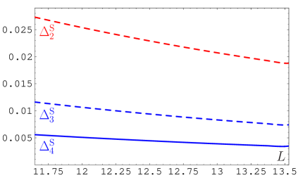
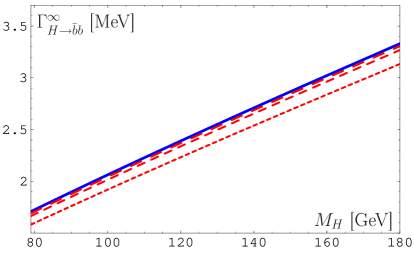
Figure 4: Left: The relative errors $\Delta_{N}[L]$ for $N=2,3$, and $4$ of the truncated FAPT expansion, given by Eq. (56), with respect to the result of the resummation procedure, represented by Eq. (55). Right: The width $\Gamma_{H\to b\bar{b}}$ as a function of the Higgs-boson mass $M_{H}$ in the resummed (blue solid line) and the truncated (at the order $N$) FAPT for three different values of $N$ represented by dashed red lines. The short-dashed line corresponds to $N=1$, the dashed one to $N=2$, and the long-dashed line to $N=3$.

To this end, we use the values of the RG-invariant masses $\hat{m}_{(1)}$ in the one-loop approximation, which we have extracted from two different sources: $\hat{m}_{b}^{(1)}=8.22$ GeV KuSt01 and $\hat{m}_{b}^{(1)}=8.53$ GeV PeSt02 , with details being provided in Appendix E.

In Fig. 4 we show the relative errors, given by (57), for $N=2$, $N=3$, and $N=4$ in the probed range of $L\in[11.7,13.6]$. We see that already $\Gamma_{H\to b\bar{b}}^{\text{\tiny FAPT}}[L;2]$ gives correct results to better than 2.5%, whereas $\Gamma_{H\to b\bar{b}}^{\text{\tiny FAPT}}[L;3]$ reaches a still better accuracy at the level of 1%. This means that, on practical grounds, there is no need to calculate further corrections, because in order to be correct at the level of 1%, it is actually sufficient to take into account only the first three coefficients up to $\tilde{d}_{3}$. This conclusion does not change if we vary the parameters of the model $P_{H}(t)$. To be more precise, varying the coefficients $\tilde{d}_{i}$ in a reasonable range—in correspondence to their order, say, about 5$\%$ for $\tilde{d}_{2}$ up to 30$\%$ for $\tilde{d}_{5}$—we induce changes of the parameter $c$ on the level of about $5\%$ which leave the main results (and conclusions) unchanged. By the same token, we can conclude that the quality of the convergence of the considered series in FAPT is quite high with a tolerance of only a few percent.

Table 4: Perturbation Theory (PT) coefficients $\tilde{d}_{n}$ for the $D_{\text{S}}$ series in the deformed versions of the model in comparison with the original one.

PT coefficients  $\tilde{d}_{1}\vphantom{{}^{|}_{|}}$ $\tilde{d}_{2}$ $\tilde{d}_{3}$ $\tilde{d}_{4}$ $\tilde{d}_{5}$  pQCD results with $N_{f}=5$ BCK05 1 7.42  62.3  620  —  Normal Model (52) with $c=2.43,~{}\delta=-0.52$ 1 7.50  61.1  625  7826  Enhanced Deformation (52) with $c=2.62,\delta=-0.50$ 1 7.85 68.5 752 10120  Reduced Deformation (52) with $c=2.25,\delta=-0.51$ 1 6.89 52.0 492 5707

Let us now expand our statements about the uncertainties of our results with regard to the model generating function $P(t)$. To this end, we deform our original model with $c=2.43$ and $\delta=-0.52$ in order to enhance or reduce the magnitude of the last known coefficient $\tilde{d}_{4}$ and the value of the still uncalculated coefficient $\tilde{d}_{5}$ (for details see Table 4). The results of this variation are shown in the left panel of Fig. 5 in the form of a strip, the upper boundary of which is formed by the enhanced version of the $P(t)$ model, whereas the lower boundary of the strip corresponds to the “reduced” version of the model. We see that the uncertainty caused by this deformation is less than 0.5%.

 

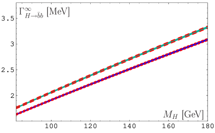
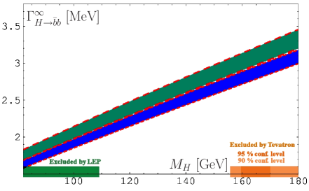
Figure 5: Left: The width $\Gamma_{H\to b\bar{b}}^{\infty}$ as a function of the Higgs-boson mass $M_{H}$ in the resummed FAPT expansion, using different models for the generating function $P(t)$—see Table 4. Right: The width $\Gamma_{H\to b\bar{b}}^{\infty}$ as a function of the Higgs-boson mass $M_{H}$ in the resummed FAPT, varying both the generating function $P(t)$ in accordance with Table 4 and also the mass $\hat{m}_{(1)}$ with $\delta\hat{m}_{(1)}=\pm 0.1$ GeV. In both panels the upper strip corresponds to the Penin–Steinhauser estimate $\hat{m}_{(1)}=8.53$ GeV PeSt02 , whereas the lower one derives from the value $\hat{m}_{(1)}=8.21$ GeV determined by Kühn and Steinhauser in Ref. KuSt01 . Here and also in Fig. 6 we indicated on the abscissa the window of the mass values of the Higgs-boson still accessible to experiment.

Now we want to discuss what changes are induced when one applies for the same kind of analysis the FAPT resummation approach at the two-loop order. In that case, there is a technical complication: The evolution factors are not simple powers $a^{\nu}[L]$, but more involved expressions like $a^{\nu_{0}}[L]\left[1+c_{1}\,a\right]^{\nu_{1}}$, as one sees by comparing with Eq. (87). For this reason, the result of the resummation is more complicated, finally amounting to Eq. (99).

Here we resort only to graphical illustrations of our results. In the left panel of Fig. 6, we discuss the convergence properties of the decay widths, truncated at the order $N$, relative to the resummed two-loop result $\Gamma_{H\to b\bar{b}}^{\infty}$. From this, we infer that our conclusions drawn from the one-loop analysis remain valid. Indeed, $\Gamma_{H\to b\bar{b}}^{\text{\tiny FAPT}}[L;2]$ is correct to better than 2%, whereas $\Gamma_{H\to b\bar{b}}^{\text{\tiny FAPT}}[L;3]$ reaches an even higher precision level of the order of 0.7%.

In the right panel of Fig. 6, we show the results for the decay width $\Gamma_{H\to b\bar{b}}^{\infty}(M_{H})$ in the resummed two-loop FAPT, in the window of the Higgs mass allowed by existing experiments—LEP and Tevatron Tevatron2010 . Comparing this outcome with the one-loop result—upper strip in the same panel of this figure—reveals a 5% reduction of the two-loop estimate. This reduction consists of two parts: one part ($\approx+7\%$) is due to the difference in the mass $\hat{m}$ in both approximations, while the other ($\approx-2\%$) comes from the difference in the values of $R_{S}(M_{H})$ in the one-loop and the two-loop approximations.

 

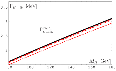
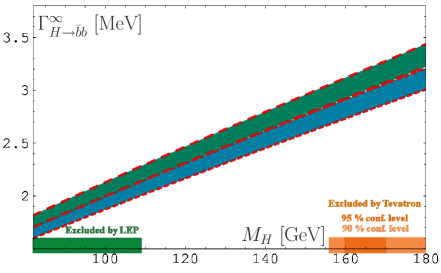
Figure 6: Left panel: The two-loop width $\Gamma_{H\to b\bar{b}}$ as a function of the Higgs boson mass $M_{H}$ in the resummed (black solid line) and the truncated (at the order $N$) FAPT. Here, the short-dashed line corresponds to $N=1$, the dashed one to $N=2$, and the long-dashed line to $N=3$. Right panel: The two-loop width $\Gamma_{H\to b\bar{b}}^{\infty}$ as a function of the Higgs-boson mass $M_{H}$ in the resummed FAPT is shown (lower strip), varying the mass in the interval $\hat{m}_{(2)}=8.22\pm 0.13$ GeV according to the Penin–Steinhauser estimate $\overline{m}_{b}(\overline{m}_{b}^{2})=4.35\pm 0.07$ GeV PeSt02 . The upper strip shows the corresponding one-loop result. The window of the mass values of the Higgs-boson which is still accessible to experiment is explicitly indicated.

In our predictions we have considered two different options for the values of the RG-effective $b$-quark mass, $\overline{m}_{b}(\overline{m}_{b}^{2})$, which we have taken from two independent analyses. One value originates from Ref. PeSt02 ($\overline{m}_{b}(\overline{m}_{b}^{2})=4.35\pm 0.07$ GeV), while the other was derived in Ref. KuSt01 yielding a somewhat deviating result, notably, $\overline{m}_{b}(\overline{m}_{b}^{2})=4.19\pm 0.05$ GeV. In Fig. 6 we show all two-loop quantities adopting for the RG-effective $b$-quark mass the result obtained by Penin and Steinhauser in Ref. PeSt02 . The relative difference between these two choices is of the order of 4%, so that squared masses differ by 7%. This means that the corresponding curves for the Kühn–Steinhauser value of $\overline{m}_{b}(\overline{m}_{b}^{2})$ KuSt01 can be actually obtained from those shown by downsizing them with an overall reduction factor of 7%. From this we conclude that the real theoretical uncertainty of the Higgs-boson width in this decay channel is de facto determined by the upper boundary of the Penin–Steinhauser estimate PeSt02 , with the lower boundary of the Kühn–Steinhauser KuSt01 being in the range of $6$% (6=(5+7)/2).

V Adler function of the vector correlator and $\bm{R_{e^{+}e^{-}\to\,\textbf{hadrons}}}$

So far, we have discussed only the Adler function related to the scalar correlator. But this sort of considerations can be applied to the vector correlator as well. To be specific, we are interested in modeling the generating function of the perturbative coefficients $\tilde{d}_{n}$ (see the first row in Table II.2) of the Adler function of the vector correlator (labeled below by the symbol V) BCK08 ; BCK10

$$D_{\text{V}}[L] = d_{0}+d_{1}\,\sum_{n=1}^{\infty}\tilde{d}_{n}\,\left(\frac{\alpha_{s}[L]}{\pi}\right)^{n}\,.$$ (58)

To account for the $n$-dependence of the coefficients $\tilde{d}_{n}$, in accordance with the asymptotic model of (46), we write

$$\tilde{d}_{n}^{\text{V}}=c^{n-1}\,\frac{\delta^{n+1}-n}{\delta^{2}-1}\,\Gamma(n)\,,$$ (59a)

which can be derived from the generating function

$$P_{\text{V}}(t) = \frac{\delta\,e^{-t/c\delta}-(t/c)\,e^{-t/c}}{c\left(\delta^{2}-1\right)}\,.$$ (59b)

Our predictions, obtained with this generating function by fitting the two known coefficients $\tilde{d}_{2}$ and $\tilde{d}_{3}$ and using the model (59), have been included in Table 5. We observe a good agreement between our estimate $\tilde{d}_{4}^{\text{V}}=27.1$ and the value 27.4, calculated recently by Chetyrkin et al. in Ref. BCK08 ; BCK10 . Would we use instead a fitting procedure, which would take into account the fourth-order coefficient $\tilde{d}_{4}$ in order to predict $\tilde{d}_{5}$, we would have to readjust the model parameters in (59) to the new values $\left\{c=3.5548,~{}\delta=1.32448\right\}$ $\to$ $\left\{c=3.5526,~{}\delta=1.32453\right\}$. These findings provide evident support for our model evaluation, and we may expect that our procedure will work in other cases as well.

In order to explore to what extent the exact knowledge of the higher-order coefficients $\tilde{d}_{n}$ is important, we employed our model (59) with different values of the parameters $c$ and $\delta$: $c=3.63$ and $\delta=1.3231$. These values are, roughly speaking, tantamount to replacing the exact value of the coefficient $\tilde{d}_{4}=27.4$ by something approximately equal to the NNA prediction obtained in BroadKa93 ; BroadKa02 . The difference between the analytic sums of the two models in the region corresponding to $N_{f}=4$ is indeed very small, reaching just a mere $0.2\%$.

Table 5: Coefficients $\tilde{d}_{n}$ for the Adler-function series with $N_{f}=4$. The numbers in the square brackets denote the lower and the upper limits of the INNA estimates.

PT coefficients  $\tilde{d}_{1}\vphantom{{}^{|}_{|}}$  $\tilde{d}_{2}$  $\tilde{d}_{3}$  $\tilde{d}_{4}$  $\tilde{d}_{5}$ 1  pQCD results with $N_{f}=4$ BCK08 ; BCK10 $1\vphantom{{}^{|}_{|}}$  1.52  2.59  27.4  —  Models and estimates 2  Model (59) with $c=3.555,~{}\delta=1.3245$ $1\vphantom{{}^{|}_{|}}$  1.52  2.59  27.1  2024 3  Model (59) with $c=3.553,~{}\delta=1.3245$ $1\vphantom{{}^{|}_{|}}$  1.52  2.60  27.3  2025 4  Model (59) with $c=3.630,~{}\delta=1.3231$ $1\vphantom{{}^{|}_{|}}$  1.53  2.26  20.7  2020 5  “NNA” prediction of BroadKa02 ; BroadKa93 $1\vphantom{{}^{|}_{|}}$  1.44  13.47  19.7  579 6  “INNA” prediction of App. C $1\vphantom{{}^{|}_{|}}$  1.44  $[3.5,9.6]$  $[20.4,48.1]$  $[674,2786]$ 7 “FAC” prediction of KaSt95 ; BCK02  8.4 $\pm 18$  152

Then, we have

$$D_{\text{V}}^{\text{APT}}[L] = 1+d_{1}\,\sum_{n\geq 1}\frac{\tilde{d}^{\text{V}}_{n}}{\pi^{n}}\,\mathcal{A}_{n}^{\text{\tiny glob}}[L]\,,$$ (60)

$$D_{\text{V}}^{\text{APT}}[L;N] = 1+d_{1}\,\sum_{n=1}^{N}\frac{\tilde{d}^{\text{V}}_{n}}{\pi^{n}}\,\mathcal{A}_{n}^{\text{\tiny glob}}[L]\,,$$ (61)

while the global-APT resummation result for $D_{\text{V}}^{\text{APT}}[L]$ is given in Appendix B by Eq. (70b). The relative errors

$$\Delta_{N}^{\text{V}}(Q^{2}) = 1-\frac{D_{\text{V}}^{\text{APT}}[\ln(Q^{2}/\Lambda^{2});N]}{D_{\text{V}}^{\text{APT}}[\ln(Q^{2}/\Lambda^{2})]}\,,$$ (62)

evaluated in the range $Q^{2}\in[2,20]$ GeV² for three values of the expansion $N=1,2,3$, are displayed in Fig. 7. We observe from this figure that already $D_{\text{V}}^{\text{APT}}[L;1]$ provides an accuracy in the vicinity of 1%, whereas $D_{\text{V}}^{\text{\tiny APT}}[L;2]$ is smaller then 0.1% in the interval $Q^{2}=1-20$ GeV². This means that there is no real need to calculate further corrections. Staying at the level of being correct to a better accuracy than 1%, it is virtually enough to take into account only the terms up to $d_{2}$. This conclusion is quite robust against the variation of the parameters of the model $P_{\text{V}}(t)$.

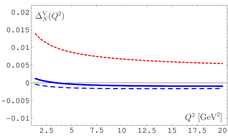
Figure 7: The relative errors $\Delta^{\text{V}}_{N}(Q^{2})$ evaluated for different values of $N$: $N=1$ (short-dashed red line), $N=2$ (solid blue line), and $N=3$ (dashed blue line) of the truncated APT given by Eq. (61), in comparison with the exact result of the resummation procedure represented by Eq. (70a).

The main outcome here may look somewhat surprising: In fact, the best order of truncation of the FAPT series in the region $Q^{2}=2-20$ GeV² is reached by employing the N²LO approximation, i.e., by keeping just the $d_{2}$-term.

VI Conclusions

In this work we have given considered in detail relations among popular perturbative approaches: FOPT, CIPT, and FAPT. We proved that in the Minkowski region both CIPT and FAPT produce for the $R$-ratios which are related to the corresponding Adler functions—see Eqs. (22)–(24)—the same results. These results do not coincide—for any fixed order of the perturbative expansion—with those obtained with FOPT.

We also considered in detail the resummation properties of non-power-series expansions within FAPT. In particular, we have given analysis of the Adler function of a scalar, $D_{S}$, and a vector, $D_{V}$, correlator presenting results at the two-loop running of the coupling. Using a particular generating function for the coefficients of the perturbative expansion, which embodies information about their asymptotic behavior, we derived results for the whole series by resumming it. We used this key feature of the non-power-series expansion within FAPT in order to reduce the theoretical uncertainties in obtaining estimates for crucial observables, like the decay width of the Higgs boson into a $b\bar{b}$ pair, relevant for the Higgs search at the Tevatron and the LHC (Sec. IV).

Employing an appropriate generating function, we estimated the values of the coefficients $\tilde{d}_{4}^{H}$ and $\tilde{d}_{5}^{H}$ and found that they are close to those computed by other groups using different perturbative methods. Moreover, we were able to resum the whole series and extract reliable predictions for the width $\Gamma_{H\to b\bar{b}}$ in terms of the Higgs-boson mass in comparison with analogous estimates at fixed orders $N=1,2,3$ of the perturbative expansion. This allowed us to gauge the accuracy of the truncation procedure of the FAPT expansion, estimating the relative errors for $N=2,3,4$. We found that the convergence of the FAPT non-power-series expansion involves uncertainties at the level of only a few percent. A cautious conclusion from this is that the reached accuracy of the order of 1% at the truncation level of N³LO is comparable with, or even slightly better than, the 2% uncertainty involved in the $\overline{m}_{b}(\overline{m}_{b}^{2})$ estimates. For this reason, there is no real need to take into account higher-order corrections.

Our Higgs-decay predictions are given in graphical form in Figs. 4 (one-loop-order running), 5 (one-loop-order running), and 6 (two-loop-order running). In Fig. 5 we presented our one-loop resummed FAPT results for two different estimates of the mass scales: $\hat{m}_{(1)}=8.53$ GeV PeSt02 (upper strip) and $\hat{m}_{(1)}=8.21$ GeV KuSt01 (lower strip). The graphical representation of the two-loop decay width in the resummed FAPT is displayed in Fig. 6—lower strip—in comparison with the one-loop result (upper strip). In this calculation we varied the mass in the interval $\hat{m}_{(2)}=8.22\pm 0.13$ GeV, implementing the Penin–Steinhauser estimate $\overline{m}_{b}(\overline{m}_{b}^{2})=4.35\pm 0.07$ GeV PeSt02 . The corresponding predictions for the other option, offered by the Kühn–Steinhauser estimate $\overline{m}_{b}(\overline{m}_{b}^{2})$ KuSt01 , can be obtained by reducing the previous results by an overall factor of about 7%. On the experimental side, one should keep in mind that the decay mode $H\to b\bar{b}$ is very challenging, but due to be measured by the ATLAS Collaboration at LHC ATLAS2010 .

In Sec. V we turned our attention to the Adler function, related to a vector correlator, in order to perform the FAPT resummation in the same manner as we did for the Higgs-boson-decay width. We used the generating function (59b) which depends on two parameters. To validate the robustness of our predictions, we varied the values of these parameters and found that this variation exerts only a small effect on the predicted value of $\tilde{d}_{5}$ and on the resummation result. It turns out that for a fixed number of flavors $N_{f}=4$, the obtained results are within the limits set by the INNA method, being, however, incompatible with both the NNA prediction of BroadKa02 ; BroadKa93 and also the FAC one KaSt95 ; BCK02 . We also estimated the influence of heavy-quark thresholds crossing in Appendix B.

Bottom line: We provided evidence in terms of two concrete examples that FAPT can provide accurate and robust estimates for relevant observables that are otherwise inaccessible by FOPT or CIPT. Moreover, using the suggested resummation approach within FAPT, we could optimize the truncation of the perturbative non-power-series expansion, thus minimizing the truncation uncertainty.

Appendix A Relations between $R$ and $D$

In this Appendix we derive expression (6) basing our reasoning on the useful relations between $R$ (LHS) and $D$ (RHS)

$$\int_{0}^{\infty}{ds\over(s+Q^{2})}\left({\mu^{2}\over s}\right)^{\delta} = {\pi\over\sin(\pi\delta)}\left({\mu^{2}\over Q^{2}}\right)^{\delta}\,;$$ (63a)

$$Q^{2}\int_{0}^{\infty}{ds\over(s+Q^{2})^{2}}\left({\mu^{2}\over s}\right)^{\delta} = {\pi\delta\over\sin(\pi\delta)}\left({\mu^{2}\over Q^{2}}\right)^{\delta}\,,$$ (63b)

worked out in BKM01 . Equation (63b) can be rewritten in the form of a dispersion relation between two specific quantities $\tilde{R}$ and $\tilde{D}$ to read

$$\hat{D}\left[\tilde{R}\right]\equiv Q^{2}\int_{0}^{\infty}{ds\over(s+Q^{2})^{2}}\tilde{R}=Q^{2}\int_{0}^{\infty}{ds\over(s+Q^{2})^{2}}\left[{\sin(\pi\delta)\over\pi\delta}\left(\frac{\mu^{2}}{s}\right)^{\delta}\right]=\left({\mu^{2}\over Q^{2}}\right)^{\delta}\,=\tilde{D}\,.~{}~{}~{}$$ (64)

From this equation we deduce the following correspondence between the terms $\tilde{R}$ (LHS) and $\tilde{D}$ (RHS):

$$\tilde{R}={\sin(\pi\delta)\over\pi\delta}\left(\frac{\mu^{2}}{s}\right)^{\delta}\Longleftrightarrow\left(\frac{\mu^{2}}{Q^{2}}\right)^{\delta}=\tilde{D}\,.$$ (65)

The powers of $\ln(Q^{2}/\mu^{2})$ in $D(Q^{2},\mu^{2})$ generate, by means of $\hat{R}\left[D\right]$ in Eq. (4), the $\pi^{2}$-terms in $R(s,\mu^{2})$. To demonstrate how this happens, we take $2k$ times derivatives with respect to the variable $\pi\delta$ on both sides of Eq. (65) and set $\delta=0$. Then, we obtain a new relation between $\tilde{D}$ and $\tilde{R}$, given by

$$\tilde{D}\to\left(\ln(Q^{2}/\mu^{2})\right)^{2k}\Longleftrightarrow(-1)^{k}\frac{(\pi^{2})^{k}}{2k+1}+\ldots\,,$$ (66)

where the ellipsis on the RHS indicates that the terms with the powers of $\ln(s/\mu^{2})$ in $R$ should, ultimately, disappear upon setting $s=\mu^{2}$, because only the even powers will survive. This can be traced back to the fact that the $\left(\ln(Q^{2}/\mu^{2})\right)^{m}$ terms in $D$ originate from the expansion of the RHS of equation d_n a^n_s(Q^2) = d_n a^n_s(μ^2) (1+a_s(μ^2)β_0 ln(Q^2/μ^2))^-n that leads to the expression

$$d_{n}\,a^{n}_{s}(Q^{2})=d_{n}\,a_{s}^{n}\sum_{m=0}\frac{(n-1+m)!}{(n-1)!~{}(m)!}(a_{s}\beta_{0}\ln(Q^{2}/\mu^{2}))^{m}\,.$$ (67)

Finally, substituting relation (66) into the expansion entering Eq. (67), one arrives at Eq. (6)

$$d_{n}\,a^{n}_{s}\to d_{n}\,a_{s}^{n}\sum_{k=0}\frac{(n-1+2k)!}{(n-1)!~{}(2k)!}(-1)^{k}\frac{(a_{s}\beta_{0}\pi)^{2k}}{2k+1}\,.$$ (68)

Appendix B Complete global expressions for $D$ and $R$

In this appendix, we derive explicit expressions for $R^{\text{\tiny glob}}[L]$ and ${D}^{\text{\tiny glob}}[L]$ valid in the global scheme of APT. The spectral density $\rho^{\text{\tiny glob}}_{n}(\sigma)$ is related to the spectral density $\bar{\rho}_{n}(\sigma;N_{f})$ SM94 ; SS96 ; Mag99 :

$$\rho^{\text{\tiny glob}}_{n}(\sigma)=\theta\left[\sigma\leq m^{2}_{4}\right]\,\bar{\rho}_{n}(\sigma;3)+\sum\limits_{f=4}^{6}\theta\left[m^{2}_{f}<\sigma\leq m^{2}_{f+1}\right]\,\bar{\rho}_{n}(\sigma;N_{f})\,,$$ (69)

where—in order to make our formulae more compact—we wrote $m_{4}=m_{c}$, $m_{5}=m_{b}$, $m_{6}=m_{t}$, and $m_{7}=+\infty$.

Then, as was shown in BM08 ; AB08gfapt , we have for

$$R^{\text{\tiny FAPT}}[L]=d_{0}\! \!+\! \!d_{1}\sum\limits_{f=3}^{6}\theta\left(L_{f}\!\leq\!L\!<\!L_{f+1}\right)\left\langle\!\!\!\left\langle{\bar{\mathfrak{A}}_{1}\!\Big{[}L\!+\!\lambda_{f}\!-\!\frac{t}{\beta_{f}};f\Big{]}}\right\rangle\!\!\!\right\rangle_{P}$$ (70a)

$$\!+\! \!d_{1}\sum\limits_{f=3}^{5}\theta\left(L_{f}\!\leq\!L\!<\!L_{f+1}\right)\sum\limits_{k=f+1}^{6}\left\langle\!\left\langle{\Delta_{k}\bar{\mathfrak{A}}_{1}[t]}\right\rangle\!\right\rangle_{P}\,;~{}~{}~{}$$

$${D}^{\text{\tiny FAPT}}[L]=d_{0}\! \!+\! \!d_{1}\,\sum\limits_{f=3}^{6}\left\langle\!\!\!\left\langle{\int_{L_{f}}^{L_{f+1}}\!\frac{\bar{\rho}_{1}\left[L_{\sigma}+\lambda_{f};N_{f}\right]\,dL_{\sigma}}{1+e^{L-L_{\sigma}-t/\beta_{f}}}}\right\rangle\!\!\!\right\rangle_{P}$$ (70b)

$$\!+\! \!d_{1}\,\sum\limits_{f=4}^{6}\left\langle\!\left\langle{\Delta_{f}[L,t]}\right\rangle\!\right\rangle_{P}\,,$$

where $\lambda_{f}\equiv\ln(\Lambda_{3}^{2}/\Lambda_{f}^{2})$ describes the shift of the logarithmic argument due to the change of the QCD scale parameter $\Lambda_{3}\to\Lambda_{f}$, (with $L_{f}\equiv\ln(m_{f}^{2}/\Lambda_{3}^{2})$), $L_{3}=-\infty$, and $L_{7}=+\infty$. The second term in Eq. (70a) presents a natural generalization of the fixed-$N_{f}$ formula (42) for the case of using different QCD scales $\Lambda_{f}$ for each fixed-$N_{f}$ interval. The last term in Eq. (70b) appears because of the continuation of $R^{\text{\tiny glob}}[L]$ at the heavy-quark thresholds:

$$\Delta_{f}\bar{\mathfrak{A}}_{1}[t]\equiv\bar{\mathfrak{A}}_{1}\!\Big{[}L_{f}+\lambda_{f}-\frac{t}{\beta_{f}};f\Big{]}-\bar{\mathfrak{A}}_{1}\!\Big{[}L_{f}+\lambda_{f-1}-\frac{t}{\beta_{f-1}};f-1\Big{]}\,.$$ (71)

In the Euclidean domain, the corrections $\left\langle\!\left\langle{\Delta_{f}[L,t]}\right\rangle\!\right\rangle_{P}$ to the naive expectation formula are defined by

$$\Delta_{f}[L,t] \equiv \int_{0}^{1}\!\frac{\bar{\rho}_{1}\left[L_{f}+\lambda_{f}-tx/\beta_{f};N_{f}\right]\,t}{\beta_{f}\,\left[1+e^{L-L_{f}-t\bar{x}/\beta_{f}}\right]}\,dx$$ (72)

$$- \int_{0}^{1}\!\frac{\bar{\rho}_{1}\left[L_{f}+\lambda_{f-1}-tx/\beta_{f-1};N_{f-1}\right]\,t}{\beta_{f-1}\,\left[1+e^{L-L_{f}-t\bar{x}/\beta_{f-1}}\right]}\,dx\,.~{}~{}~{}$$

In contrast to the Minkowski case, they explicitly depend on $L$.

Consider now the extension of these summation techniques to global FAPT, i.e., when one takes into account heavy-quark thresholds. To be more precise, we will deal with the summation of the following series:

$${D_{\nu}^{\text{\tiny FAPT}}[L]\choose R_{\nu}^{\text{\tiny FAPT}}[L]}=d_{0}{\mathcal{A}^{\text{\tiny glob}}_{\nu}[L]\choose\mathfrak{A}^{\text{\tiny glob}}_{\nu}[L]}+d_{1}\,\sum_{n=1}^{\infty}\tilde{d}_{n}\,{\mathcal{A}^{\text{\tiny glob}}_{n+\nu}[L]\choose\mathfrak{A}^{\text{\tiny glob}}_{n+\nu}[L]}\,.$$ (73)

Note that due to the different relative normalization of $\mathcal{A}_{n+\nu}[L]$ ($\mathfrak{A}_{n+\nu}[L]$) and $\mathcal{A}^{\text{\tiny glob}}_{n+\nu}[L]$ ($\mathfrak{A}^{\text{\tiny glob}}_{n+\nu}[L]$), the coefficients $\tilde{d}_{n}$ in Eqs. (33) and (73) are also different. In order to obtain a generalization of the resummation procedure, given by Eq. (44), we propose to apply it to the spectral densities $\rho_{n+\nu}^{\text{\tiny glob}}[L_{\sigma}]$. This will be done for every $N_{f}$-fixed integration region causing its reduction to $\bar{\rho}_{n+\nu}[L_{\sigma}+\lambda_{f};N_{f}]$. Subsequently, application of Eq. (44) to sum up the series $\sum\limits_{n\geq 1}\bar{\rho}_{n+\nu}[L_{\sigma}+\lambda_{f};N_{f}]\left\langle\!\left\langle{t^{n-1}}\right\rangle\!\right\rangle_{P}$ will yield

$$\sum\limits_{n\geq 1}\bar{\rho}_{n+\nu}[L_{\sigma}+\lambda_{f};N_{f}]\left\langle\!\left\langle{t^{n-1}}\right\rangle\!\right\rangle_{P} = \left\langle\!\!\!\left\langle{\bar{\rho}_{1+\nu}\left[L_{\sigma}+\lambda_{f}-\frac{t}{\beta_{f}};N_{f}\right]}\right\rangle\!\!\!\right\rangle_{P_{\nu}}\,.$$ (74)

As shown in BM08 , this procedure generates in the Minkowski region the following answer for the analytic image of the entire sum:

$$R_{\nu}^{\text{\tiny FAPT}}[L]=d_{0}\,{\mathfrak{A}}^{\text{\tiny glob}}_{\nu}[L]\! \!+\! \!d_{1}\sum\limits_{f=3}^{6}\theta\left(L_{f}\!\leq\!L\!<\!L_{f+1}\right)\left\langle\!\!\!\left\langle{\bar{\mathfrak{A}}_{1+\nu}\!\Big{[}L\!+\!\lambda_{f}\!-\!\frac{t}{\beta_{f}};f\Big{]}}\right\rangle\!\!\!\right\rangle_{P_{\nu}}$$ (75)

$$\!+\! \!d_{1}\sum\limits_{f=3}^{6}\theta\left(L_{f}\!\leq\!L\!<\!L_{f+1}\right)\!\!\sum\limits_{k=f+1}^{6}\!\left\langle\!\left\langle{\Delta_{k}\bar{\mathfrak{A}}_{1+\nu}[t]}\right\rangle\!\right\rangle_{P_{\nu}}~{}$$

with $P_{\nu}(t)$ taken from Eq. (45).

Appendix C Improved Naive Non-Abelization procedure

Following the analysis of Ref. MS04 , we consider an expansion of the perturbative coefficients $d_{n}$ in a power series in $b_{0},b_{1},\ldots$, i.e.,

$$\tilde{d}_{3}=b_{0}^{2}\,d_{3}[2,0]+b_{1}\,d_{3}[0,1]+b_{0}\,d_{3}[1,0]+d_{3}[0,0]\,,$$

as opposed to the standard expansion in a power series in $N_{f}$ (i.e., the number of flavors), ~d_3= N_f^2   d_3(2)+N_f^1  d_3(1)+N_f^0  d_3(0). Here, the first argument $n_{0}$ of the coefficients $d_{n}[n_{0},n_{1},\ldots]$ corresponds to the power of $b_{0}$, whereas the second one $n_{1}$ refers to the power of $b_{1}$, etc. The coefficient $d_{n}[0,0,\ldots,0]$ represents the “genuine” corrections which are associated with the coefficients $b_{i}$ in the power $n_{i}=0$. If all the arguments of the coefficient $d_{n}[\ldots,m,0,\ldots,0]$ to the right of the index $m$ are equal to zero, then, for the sake of a simplified notation, we will omit these arguments and write instead $d_{n}[\ldots,m]$. Applying this terminology, we obtain the following representation for the next few coefficients

$$\tilde{d}_{3} = b_{0}^{2}\,\underline{d_{3}[2]}+b_{1}\,\underline{d_{3}[0,1]}+b_{0}\,d_{3}[1]+d_{3}[0]\,,$$ (76)

$$\tilde{d}_{4} = b_{0}^{3}\,\underline{d_{4}[3]}+b_{1}\,b_{0}\,\underline{d_{4}[1,1]}+b_{2}\,\underline{d_{4}[0,0,1]}+b_{0}^{2}\,d_{4}[2]+b_{1}\,d_{4}[0,1]+b_{0}\,d_{4}[1]+d_{4}[0]\,,$$ (77)

$$\tilde{d}_{5} = b_{0}^{4}\,\underline{d_{5}[4]}+b_{1}\,b_{0}^{2}\,\underline{d_{5}[2,1]}+b_{1}^{2}\,\underline{d_{5}[0,2]}+b_{0}\,b_{2}\,\underline{d_{5}[1,0,1]}+b_{3}\,\underline{d_{5}[0,0,0,1]}+O\!\left(b_{0}^{3}\right).$$ (78)

The same ordering of the $\beta$-function elements applies with respect to the higher coefficients $d_{n}$ as well. Employing the standard NNA approximation, one estimates $\tilde{d}_{n}$ from the first term in the equations above, namely, $\tilde{d}_{n}\simeq b_{0}^{n}\underline{d_{n}[n-1]}$. We are going to improve this estimate by including other terms of the same order as $b_{0}^{n}$ by means of the relation $b_{i}\simeq O(b_{0}^{(i+1)})$. [For the reader’s convenience, we have underlined the coefficients of these terms in Eqs. (76)–(78).] Note that in the $\overline{\text{MS}}$ scheme, the proportionality coefficients $c_{i}=b_{i}/b_{0}^{(i+1)}$ are

$$c_{1}\approx 0.74\,;~{}~{}c_{2}\approx 0.7\,;~{}~{}c_{3}\approx 1.82\,;~{}~{}c_{4}=\text{unknown}\,.$$ (79)

All these coefficients are of order unity and their values have been estimated for $N_{f}=4$, meaning that there is no reason to neglect them in Eqs. (76)–(78). This observation allows one to generalize the large $b_{0}$-approximation, by taking into account all terms with the underlined coefficients in Eqs. (76)–(78) that belong to the same order in $b_{0}$. Within this setup, the element $\underline{d_{n}[n-1]}$ can be easily obtained from the term $d_{n}(n-1)$, i.e., via $\underline{d_{n}[n-1]}=\left(-\frac{3}{2}\right)^{n-1}d_{n}(n-1)$. Moreover, the coefficients $d_{n}(n-1)$, related to the vector correlator, and the sum rules pertaining to deep-inelastic scattering were obtained for any $n$ in BroadKa93 ; BroadKa02 , respectively.

The determination of the remaining underlined elements in Eqs. (76)–(78) is a difficult task that has been partially carried out in MS04 for the particular case of the Adler $D$-function in the representation of Eq. (76). Strictly speaking, it was found that $\underline{d_{3}[0,1]}\approx-0.4\,\underline{d_{3}[2]}$ and $\underline{d_{3}[0,1]}\approx 1.2$, and it was proved that both elements are of order unity. With this in mind, we propose to use in the expansions of $D_{S}$, [cf. (51)], and $D_{V}$,  [cf. (58)], the following relation for the considered coefficients

$$\big{|}\underline{d_{n}[n_{0},n_{1},\ldots]}\big{|}=\big{|}\underline{d_{n}[n-1]}\big{|}\,.$$ (80)

Surprisingly, this rough approximation leads to reasonable results for the coefficients $d_{n}$ (especially when compared with those found with the NNA method), as one can see from the entries dubbed “INNA” in Tables II.2, 3, 5. As an illustrative example of this procedure, use Eq. (80) in Eq. (77) to predict the coefficients

$$\tilde{d}_{4}\approx\tilde{d}^{\text{INNA}}_{4} = d_{4}[3]\left(b_{0}^{3}+b_{1}b_{0}\pm b_{2}\right)+O(b_{0}^{2})$$ (81)

$$\tilde{d}_{5}\approx\tilde{d}^{\text{INNA}}_{5} = d_{5}[4]\left(b_{0}^{4}+b_{1}b_{0}^{2}+b_{1}^{2}+b_{0}\,b_{2}\pm b_{3}\right)+O(b_{0}^{3})\,,$$ (82)

with their values being given in Tables 3 and 5. This kind of approximation is based upon the condition (80) and is in line with the underlying assumptions of the original NNA procedure.

Appendix D Two-loop results

D.1 Recurrence relations

The expansion of the $\beta$-function in the two-loop approximation is given by

$$\frac{d}{dL}\left(\frac{\alpha_{s}[L]}{4\pi}\right)=-b_{0}\left(\frac{\alpha_{s}[L]}{4\pi}\right)^{2}-b_{1}\left(\frac{\alpha_{s}[L]}{4\pi}\right)^{3}\,,$$ (83)

where $L=\ln(\mu^{2}/\Lambda^{2})$ and

$$b_{0}=\frac{11}{3}\,C_{\text{A}}-\frac{4}{3}\,T_{\text{R}}N_{f}\,,\qquad\qquad b_{1}=\frac{34}{3}\,C_{\text{A}}^{2}-\left(4C_{\text{F}}+\frac{20}{3}\,C_{\text{A}}\right)T_{\text{R}}N_{f}$$ (84)

with $C_{\text{F}}=\left(N_{\text{c}}^{2}-1\right)/2N_{\text{c}}=4/3$, $C_{\text{A}}=N_{\text{c}}=3$, $T_{\text{R}}=1/2$, and $N_{f}$ denoting the number of active flavors. Then, the corresponding two-loop equation for the coupling $a=b_{0}\,\alpha/(4\pi)$ reads

$$\frac{da_{(2)}[L]}{dL}=-a_{(2)}^{2}[L]\left(1+c_{1}\,a_{(2)}[L]\right)\quad\text{with}~{}c_{1}\equiv\frac{b_{1}}{b_{0}^{2}}\,.$$ (85)

Still higher beta-function coefficients, e.g., $b_{2}$, $b_{3}$, can be found in vRVL97 ; MS04 . This equation immediately generates the following recurrence relation

$$-\frac{1}{n}\,\frac{da_{(2)}^{n}[L]}{dL}=a_{(2)}^{n+1}[L]+c_{1}\,a_{(2)}^{n+2}[L]$$ (86a)

for consecutive powers of the coupling constant. Due to its linearity, this relation remains valid also for the analytic images of the coupling’s powers:

$$-\frac{1}{n}\,\frac{d}{dL}\,\mathcal{F}_{n}[L]=\mathcal{F}_{n+1}[L]+c_{1}\,\mathcal{F}_{n+2}[L]\,,$$ (86b)

where, as it has already been used in Sec. III, $${\mathcal{F}}[L] \mathcal{A}^{(2)}[L],~{}\mathfrak{A}^{(2)}[L] \rho^{(2)}[L]$$ denotes one of the analytic quantities , or . Quite analogously, we obtain the following generalization of this relation, pertaining to fractional coupling-constant indices, viz.,

$$-\frac{1}{n+\nu}\,\frac{d}{dL}\,\mathcal{F}_{n+\nu}[L]=\mathcal{F}_{n+1+\nu}[L]+c_{1}\,\mathcal{F}_{n+2+\nu}[L]\,.$$ (86c)

In the two-loop approximation we have a different evolution for the running mass, which reads

$$\bar{m}_{b}^{2}(Q^{2}) = \hat{m}_{(2)}^{2}\,\left[\alpha_{s}^{(2)}(Q^{2})\right]^{\nu_{0}}\left[1+\frac{c_{1}\,b_{0}}{4\,\pi}\,\alpha_{s}^{(2)}(Q^{2})\right]^{\nu_{1}}$$ (87a)

$$= \hat{m}_{(2)}^{2}\,\left[\frac{4\,\pi}{b_{0}}\,a_{(2)}(Q^{2})\right]^{\nu_{0}}\left[1+c_{1}\,a_{(2)}(Q^{2})\right]^{\nu_{1}}\,,$$ (87b)

where

$$\nu_{1}=2\left(\frac{\gamma_{1}}{b_{1}}-\frac{\gamma_{0}}{b_{0}}\right)$$ (88)

and $\hat{m}_{(2)}$ is the renormalization-group-invariant mass.

D.2 Resummation in FAPT for fixed $N_{f}$

Consider here the following power series with $\nu\geq 0$:

$$\mathcal{W}_{\nu}[L;t;\mathcal{F}]\equiv\sum\limits_{n\geq 1}t^{n-1}\mathcal{F}_{n+\nu}[L]$$ (89)

noting that for $\nu=0$ we would obtain the corresponding two-loop APT expression. Multiplying both sides of Eq. (86c) with $t^{n+\nu}$ and summing over $n$ from $n=1$ to $\infty$, we arrive at

$$-\hat{p}\!\int\limits_{0}^{t}\!t^{\prime\nu}\,\mathcal{W}_{\nu}[L;t^{\prime};\mathcal{F}]\,dt^{\prime}=t^{\nu}\,\left[\left(1+\frac{c_{1}}{t}\right)\,\left(\mathcal{W}_{\nu}[L;t;\mathcal{F}]-\mathcal{F}_{1+\nu}[L]\right)-c_{1}\,\mathcal{F}_{2+\nu}[L]\right]\,,$$

where $\hat{p}\equiv d/dL$. Differentiating this equation with respect to $t$, we obtain

$$\frac{d}{dt}\left\{t^{\nu}\left[\left(1+\frac{c_{1}}{t}\right)\,\left(\mathcal{W}_{\nu}[L;t;\mathcal{F}]-\mathcal{F}_{1+\nu}[L]\right)-c_{1}\,\mathcal{F}_{2+\nu}[L]\right]\right\}+\hat{p}\,t^{\nu}\,\mathcal{W}_{\nu}[L;t;\mathcal{F}]=0$$ (90)

with the initial condition $\mathcal{W}_{\nu}[L;0;\mathcal{F}]=\mathcal{F}_{1+\nu}[L]$. In order to solve this equation, we consider the following function

$$\mathcal{X}_{\nu}[L;t] \equiv \left(1+\frac{c_{1}}{t}\right)\sum\limits_{n\geq 2}t^{n+\nu-1}\mathcal{F}_{n+\nu}[L]-c_{1}\,t^{\nu}\mathcal{F}_{2+\nu}[L]\,,$$ (91a)

$$\mathcal{X}_{\nu}[L;0] = 0\,.$$ (91b)

Our initial series $\mathcal{W}[L;t;\mathcal{F}]$ is related to this function by the evident relation

$$\mathcal{W}_{\nu}[L;t;\mathcal{F}] = \mathcal{F}_{1+\nu}[L]+\frac{t^{1-\nu}}{c_{1}+t}\,\mathcal{X}_{\nu}[L;t]+\frac{c_{1}\,t}{c_{1}+t}\,\mathcal{F}_{2+\nu}[L]\,.$$ (92)

Hence, we find

$$\frac{d}{dt}\,\mathcal{X}_{\nu}[L;t]+\hat{p}\,\frac{t}{c_{1}+t}\,\mathcal{X}_{\nu}[L;t] = -\hat{p}\,t^{\nu}\,\mathcal{F}_{1+\nu}[L]-\hat{p}\,\frac{c_{1}\,t^{1+\nu}}{c_{1}+t}\,\mathcal{F}_{2+\nu}[L]\,.$$

Finally, using the substitution

$$\mathcal{X}_{\nu}[L;t]=e^{-\hat{p}\tau(t)}X_{\nu}[L;t]\,,$$ (93)

we get

$$\frac{dX_{\nu}[L;t]}{dt}=-\hat{p}\,e^{\hat{p}\tau(t)}\left(t^{\nu}\,\mathcal{F}_{1+\nu}[L]+\frac{c_{1}\,t^{1+\nu}}{c_{1}+t}\,\mathcal{F}_{2+\nu}[L]\right)\,.$$

That implies the relations

$$X_{\nu}[L;t] = -t^{1+\nu}\!\int\limits_{0}^{1}\!z^{\nu}\,dz\,\left[\frac{d\mathcal{F}_{1+\nu}[L+\tau(t\,z)]}{dL}+\frac{c_{1}\,t\,z}{c_{1}+t\,z}\,\frac{d\mathcal{F}_{2+\nu}[L+\tau(t\,z)]}{dL}\right]\,;$$

$$t^{-\nu}\mathcal{X}_{\nu}[L;t] = -t\!\int\limits_{0}^{1}\!z^{\nu}dz\,\left[\frac{d\mathcal{F}_{1+\nu}[L+\tau(t\,z)-\tau(t)]}{dL}+\frac{c_{1}\,t\,z}{c_{1}+t\,z}\,\frac{d\mathcal{F}_{2+\nu}[L+\tau(t\,z)-\tau(t)]}{dL}\right]\,,$$

where we took into account that $\hat{p}=d/dL$ and where we used the initial condition (91b). Making use of this solution in Eq. (92), we obtain

$$\mathcal{W}_{\nu}[L;t;\mathcal{F}] = \mathcal{F}_{1+\nu}[L]+\frac{t}{c_{1}+t}\,\Big{\{}c_{1}\,\mathcal{F}_{2+\nu}[L]-t\!\int\limits_{0}^{1}\!z^{\nu}dz\,\Big{[}\frac{d\mathcal{F}_{1+\nu}[L+\tau(t\,z)-\tau(t)]}{dL}~{}~{}~{}~{}~{}~{}~{}~{}~{}~{}~{}$$

$$~{}~{}~{}~{}~{}~{}~{}~{}~{}~{}~{}~{}~{}~{}~{}~{}~{}~{}~{}~{}~{}~{}~{}~{}~{}~{}~{}~{}~{}~{}~{}~{}~{}~{}~{}~{}~{}~{}+\frac{c_{1}\,t\,z}{c_{1}+t\,z}\,\frac{d\mathcal{F}_{2+\nu}[L+\tau(t\,z)-\tau(t)]}{dL}\Big{]}\Big{\}}\,.$$

Note that this equation can be recast in the equivalent form

$$\mathcal{W}_{\nu}[L;t;\mathcal{F}] = \mathcal{F}_{1+\nu}[L]-\frac{t^{2}}{c_{1}+t}\!\int\limits_{0}^{1}\!z^{\nu}dz\,\frac{d\mathcal{F}_{1+\nu}[L+\tau(t\,z)-\tau(t)]}{dL}$$ (94)

$$+ \frac{c_{1}\,t}{c_{1}+t}\,\Big{\{}\mathcal{F}_{2+\nu}[L-\tau(t)]\,\delta_{0,\nu}+\nu\!\int\limits_{0}^{1}\!z^{\nu-1}\,\mathcal{F}_{2+\nu}[L+\tau(t\,z)-\tau(t)]\,dz\Big{\}}\,,~{}~{}~{}$$

with $\delta_{0,\nu}$ being a Kronecker delta symbol. The reason for this recasting is that it is more appropriate for realizing the limit $c_{1}\to 0$ and obtain this way the one-loop expressions, given by Eqs. (44)–(45). We observe that the analytic sum of the initial power series in $t$ can be represented by means of the analytic couplings $\mathcal{F}_{1+\nu}[L]$ and $\mathcal{F}_{2+\nu}[L]$. Setting $\nu=0$, we obtain the corresponding two-loop APT expression

$$\mathcal{W}_{0}[L;t;\mathcal{F}] = \mathcal{F}_{1}[L]-\frac{t}{c_{1}+t}\!\int\limits_{0}^{t}\!\frac{d\mathcal{F}_{1}[L+\tau(t^{\prime})-\tau(t)]}{dL}\,dt^{\prime}+\frac{c_{1}\,t}{c_{1}+t}\,\mathcal{F}_{2}[L-\tau(t)]\,.~{}~{}$$ (95)

Hence, the sum expressed via equations like (44) can be recast in convolution form to read

$$\mathcal{S}_{\nu}[L]=d_{0}\mathcal{F}_{\nu}[L]+d_{1}\,\left\langle\!\!\!\left\langle\mathcal{F}_{1+\nu}[L]+\frac{c_{1}\,t}{c_{1}+t}\,\mathcal{F}_{2+\nu}[L-\tau(t)]\,\delta_{0,\nu}\right\rangle\!\!\!\right\rangle_{\!\!\!P}~{}~{}~{}~{}~{}~{}~{}~{}~{}~{}~{}~{}~{}~{}~{}~{}~{}~{}~{}$$ (96)

$$~{}+\left\langle\!\!\!\left\langle\frac{-\,d_{1}\,t^{2}}{c_{1}+t}\,\int\limits_{0}^{1}\!z^{\nu}dz\,\left\{\frac{d\mathcal{F}_{1+\nu}[L+\tau(t\,z)-\tau(t)]}{dL}+\frac{c_{1}\,\nu}{t\,z}\,\mathcal{F}_{2+\nu}[L+\tau(t\,z)-\tau(t)]\right\}\right\rangle\!\!\!\right\rangle_{\!\!\!P}\,.$$

On the other hand, for the APT case with $\nu=0$, expressions like (33) can be rewritten as

$$\mathcal{S}[L]=d_{0}+d_{1}\,\left\langle\!\!\!\left\langle\mathcal{F}_{1}[L]-\frac{t}{c_{1}+t}\!\int\limits_{0}^{t}\!\frac{d\mathcal{F}_{1}[L+\tau(t^{\prime})-\tau(t)]}{dL}\,dt^{\prime}+\frac{c_{1}\,t}{c_{1}+t}\,\mathcal{F}_{2}[L-\tau(t)]\right\rangle\!\!\!\right\rangle_{\!\!\!P}\,.~{}~{}~{}~{}~{}$$ (97)

Quite analogously it is possible to resum also the following expression

$$\mathcal{E}_{\nu;\nu_{1}}[L]=d_{0}\,\mathcal{B}_{\nu;\nu_{1}}[L]+d_{1}\sum_{n=0}^{\infty}\frac{\left\langle\!\left\langle{(-t)^{n}}\right\rangle\!\right\rangle_{P}}{n!}\,\mathcal{B}_{n+1+\nu;\nu_{1}}[L]\,,~{}$$ (98)

in which $\mathcal{B}_{\nu;\nu_{1}}[L]=\textbf{A}_{E,M}\left[a_{(2)}^{\nu}[L]\left(1+c_{1}\,a_{(2)}\right)^{\nu_{1}}[L]\right]$ is the analytic image of the two-loop evolution factor (87). Then, the FAPT result for the resummation of this series is

$$\mathcal{E}_{\nu;\nu_{1}}[L]\! \!=\! \!d_{0}\mathcal{B}_{\nu;\nu_{1}}[L]+d_{1}\,\left\langle\!\!\!\left\langle\mathcal{B}_{1+\nu;\nu_{1}}[L]+\frac{c_{1}\,t}{c_{1}+t}\,\mathcal{B}_{2+\nu;\nu_{1}}[L]\right\rangle\!\!\!\right\rangle_{\!\!\!P}$$ (99)

$$\!-\! \!\left\langle\!\!\!\left\langle\frac{d_{1}\,t^{2}}{(c_{1}+t)^{1-\nu_{1}}}\,\int\limits_{0}^{1}\!dz\,\frac{z^{\nu+\nu_{1}}}{(c_{1}+t\,z)^{\nu_{1}}}\frac{d\mathcal{B}_{1+\nu;\nu_{1}}[L+\tau(t\,z)-\tau(t)]}{dL}\right\rangle\!\!\!\right\rangle_{\!\!\!P}~{}~{}~{}$$

$$\!-\! \!\left\langle\!\!\!\left\langle\frac{d_{1}\,c_{1}\,t}{(c_{1}+t)^{1-\nu_{1}}}\,\int\limits_{0}^{1}\!dz\,\frac{z^{\nu+\nu_{1}}}{(c_{1}+t\,z)^{\nu_{1}}}\frac{t^{2}\,z}{c_{1}+t\,z}\,\frac{d\mathcal{B}_{2+\nu;\nu_{1}}[L+\tau(t\,z)-\tau(t)]}{dL}\right\rangle\!\!\!\right\rangle_{\!\!\!P}$$

$$\!+\! \!\left\langle\!\!\!\left\langle\frac{d_{1}\,c_{1}\,t^{2}}{(c_{1}+t)^{1-\nu_{1}}}\,\int\limits_{0}^{1}\!dz\,\frac{\nu_{1}\,z^{\nu+\nu_{1}}}{(c_{1}+t\,z)^{1+\nu_{1}}}\,\mathcal{B}_{2+\nu;\nu_{1}}[L+\tau(t\,z)-\tau(t)]\right\rangle\!\!\!\right\rangle_{\!\!\!P}\,.~{}~{}~{}$$

Using the exact derivative expression

$$\frac{d\mathcal{B}_{2+\nu;\nu_{1}}[L+\tau(t\,z)-\tau(t)]}{dz}=\left(\frac{t^{2}\,z}{c_{1}+t\,z}\right)\frac{d\mathcal{B}_{2+\nu;\nu_{1}}[L+\tau(t\,z)-\tau(t)]}{dL}$$

and integrating by parts we can rewrite (99) in a more convenient way to read

$$\mathcal{E}_{\nu;\nu_{1}}[L] \!=\! d_{0}\,\mathcal{B}_{\nu;\nu_{1}}[L]+d_{1}\left\langle\!\!\!\left\langle\mathcal{B}_{1+\nu;\nu_{1}}[L]+\delta_{0,{\nu+\nu_{1}}}\,t\,\left[\frac{c_{1}}{c_{1}+t}\right]^{1-\nu_{1}}\mathcal{B}_{2+\nu;\nu_{1}}[L-\tau(t)]\right\rangle\!\!\!\right\rangle_{\!\!\!P}$$ (100)

$$\!-\! \!\left\langle\!\!\!\left\langle\frac{d_{1}\,t^{2}}{(c_{1}+t)^{1-\nu_{1}}}\,\int\limits_{0}^{1}\!dz\,\frac{z^{\nu+\nu_{1}}}{(c_{1}+t\,z)^{\nu_{1}}}\frac{d\mathcal{B}_{1+\nu;\nu_{1}}[L+\tau(t\,z)-\tau(t)]}{dL}\right\rangle\!\!\!\right\rangle_{\!\!\!P}~{}~{}~{}$$

$$\!+\! \!\left\langle\!\!\!\left\langle\frac{d_{1}\,c_{1}\,t}{(c_{1}+t)^{1-\nu_{1}}}\,\int\limits_{0}^{1}\!dz\,\frac{(\nu+\nu_{1})\,z^{\nu+\nu_{1}-1}}{(c_{1}+t\,z)^{\nu_{1}}}\,\mathcal{B}_{2+\nu;\nu_{1}}[L+\tau(t\,z)-\tau(t)]\right\rangle\!\!\!\right\rangle_{\!\!\!P}\,.$$

D.3 Resummation in global FAPT

The formalism developed in the text and the previous appendices can be applied to the global case using spectral densities, which correspond to a fixed number of active flavors $N_{f}$, and are defined in the integration intervals $L_{f}<L_{\sigma}\leq L_{f+1}$. Indeed, employing $\mathcal{F}_{\nu}[L]=\rho_{\nu}[L]$ and $L=L_{\sigma}$, we can first perform the resummation before carrying out the spectral integration over $L_{\sigma}$.

Let us study these operations in some more detail within the Euclidean FAPT. In that case, the global spectral density $\rho^{\text{\tiny glob}}_{n+\nu}(\sigma)$ has the form specified in Eq. (69). It can be rewritten in an equivalent way to read

$$\rho^{\text{\tiny glob}}_{n+\nu}[L_{\sigma}]=\sum\limits_{f=3}^{6}\theta\left[L_{f}<L_{\sigma}\leq L_{f+1}\right]\,\bar{\rho}_{n+\nu}[L_{\sigma}+\lambda_{f};N_{f}]\,,$$ (101)

where we used $L_{3}=-\infty$ and $L_{7}=+\infty$. Then, we have for the sum of the global power series (in $t$) the following expression

$$\mathcal{W}^{\text{\tiny FAPT}}_{\nu}[L;t]\equiv\sum\limits_{n\geq 1}t^{n-1}\mathcal{A}^{\text{\tiny glob}}_{n+\nu}[L]=\sum\limits_{f=3}^{6}\int_{L_{f}}^{L_{f+1}}\!\frac{\rho_{\nu}^{\text{sum}}\left[L_{\sigma}+\lambda_{f};N_{f};t\right]\,dL_{\sigma}}{1+e^{L-L_{\sigma}}}$$ (102)

in which the following abbreviation was used:

$$\rho_{\nu}^{\text{sum}}\left[L;N_{f};t\right] \equiv \sum\limits_{n\geq 1}t^{n-1}\bar{\rho}_{n+\nu}[L;N_{f}]=\left(\frac{1}{\beta_{f}}\right)^{1+\nu}\sum\limits_{n\geq 1}\left[\frac{t}{\beta_{f}}\right]^{n-1}\rho_{n+\nu}[L]\,.$$ (103)

We see that this series has the form of Eq. (89) and is equal to

$$\rho_{\nu}^{\text{sum}}\left[L;N_{f};t\right] = \left(\frac{1}{\beta_{f}}\right)^{1+\nu}\,\mathcal{W}_{\nu}\left[L;\frac{t}{\beta_{f}};\rho^{(2)}\right]\,,$$ (104)

where the last argument $\rho^{(2)}$ of $\mathcal{W}_{\nu}$ means that everywhere in Eq. (94) one should substitute $\mathcal{F}[L]\to\rho^{(2)}[L]$. Hence, the initial sum

$$D^{\text{\tiny FAPT}}_{\nu}[L]\equiv d_{0}\mathcal{A}^{\text{\tiny glob}}_{\nu}[L]+d_{1}\,\sum\limits_{n\geq 1}\left\langle\!\left\langle{t^{n-1}\mathcal{A}^{\text{\tiny glob}}_{n+\nu}[L]}\right\rangle\!\right\rangle_{\!P}$$ (105)

can be resummed in the following final form

$$D^{\text{\tiny FAPT}}_{\nu}[L] = d_{0}\mathcal{A}^{\text{\tiny glob}}_{\nu}[L]+d_{1}\,\sum\limits_{f=3}^{6}\int_{L_{f}}^{L_{f+1}}\!\frac{\rho_{\nu}^{\text{sum}}\left[L_{\sigma}+\lambda_{f};N_{f}\right]\,dL_{\sigma}}{1+e^{L-L_{\sigma}}}$$ (106a)

$$\rho_{\nu}^{\text{sum}}\left[L;N_{f}\right] \equiv \left(\frac{1}{\beta_{f}}\right)^{1+\nu}\,\left\langle\!\!\!\left\langle\mathcal{W}_{\nu}\left[L;\frac{t}{\beta_{f}};\rho^{(2)}\right]\right\rangle\!\!\!\right\rangle_{\!\!\!P}\,.$$ (106b)

Appendix E Pole and RG-invariant masses of the bottom quark

We start our considerations by writing down the relation ChSt99 ; ChSt00 between the pole mass of the $b$ quark, $m_{b}$, on one hand, and the value of the running mass at the scale $\mu_{*}=\overline{m}_{b}(\mu_{*}^{2})$, which we call $\overline{m}_{b}(\overline{m}_{b}^{2})$, on the other hand:

$$\left[\frac{\overline{m}_{b}(\overline{m}_{b}^{2})}{m_{b}}\right]^{2}=1-\frac{8}{3}\,\frac{\alpha_{s}\left(m_{b}^{2}\right)}{\pi}-13.234\,\left[\frac{\alpha_{s}\left(m_{b}^{2}\right)}{\pi}\right]^{2}\,.$$ (107)

Note that some authors prefer another version of this relation in which the pole mass $m_{b}$ is used as argument in the numerator of the left-hand side: $\overline{m}_{b}(m_{b}^{2})$—see ChSt99 ; ChSt00 ; GBGS90 ; KK08 .

The QCD scales are fixed via the normalization of the strong coupling in the corresponding one- or two-loop approximation at the $Z$-pole, employing the condition $R_{e^{+}e^{-}\to\text{hadrons}}(\alpha_{s}(m_{Z}^{2}))=1.039$, suggested in BCK08 , where

$$R_{e^{+}e^{-}\to\text{hadrons}}(\alpha_{s}) = 1+\frac{\alpha_{s}}{\pi}+1.4097\,\left(\frac{\alpha_{s}}{\pi}\right)^{2}\,.$$ (108)

Table 6: The values of the QCD scale parameters $\Lambda_{f}$ and $b$-quark masses pertaining to KuSt01 .

 Loop order  $\Lambda_{3}$ [MeV]  $\Lambda_{5}$ [MeV]  $\overline{m}_{b}(\overline{m}_{b}^{2})$ [GeV]  ${m_{b}}$ [GeV]  $\hat{m}_{b}$ [GeV] 1-loop 184 115 4.21 4.69 8.22 2-loop 346 195 4.19 4.84 7.89

Table 7: The values of the $b$-quark masses employing the estimates of the Penin–Steinhauser paper PeSt02 .

 Loop order  $\Lambda_{3}$ [MeV]  $\Lambda_{5}$ [MeV]  $\overline{m}_{b}(\overline{m}_{b}^{2})$ [GeV]  ${m_{b}}$ [GeV]  $\hat{m}_{b}$ [GeV] 1-loop 184 115 4.35 4.84 8.53 2-loop 346 195 4.34 5.00 8.22

Tables 6 and 7 show the results for $\hat{m}_{b}$ obtained in this work. In parallel, we present results for the pole mass $m_{b}$, using as input the estimates for $\overline{m}_{b}(\overline{m}_{b}^{2})$ derived by Kühn and Steinhauser in Ref. KuSt01 —Table 6. In Table 7 we present analogous results, determining $\hat{m}_{b}$ from the estimates for $\overline{m}_{b}(\overline{m}_{b}^{2})$ derived by Penin and Steinhauser PeSt02 . For the sake of completeness, we also quote here the recent estimates $\overline{m}_{b}(\overline{m}_{b}^{2})=4.163\pm 0.016$ GeV Chet09 and $\overline{m}_{b}(\overline{m}_{b}^{2})=4.164\pm 0.025$ GeV Kuhn08 .

References

• (1) D. V. Shirkov and I. L. Solovtsov, Phys. Rev. Lett. 79, 1209 (1997).
• (2) A. V. Radyushkin, JINR Rapid Commun. 78, 96 (1996); [JINR Preprint, E2-82-159, 26 Febr. 1982].
• (3) N. V. Krasnikov and A. A. Pivovarov, Phys. Lett. B116, 168 (1982).
• (4) K. A. Milton and I. L. Solovtsov, Phys. Rev. D55, 5295 (1997).
• (5) K. A. Milton and O. P. Solovtsova, Phys. Rev. D57, 5402 (1998).
• (6) I. L. Solovtsov and D. V. Shirkov, Phys. Lett. B442, 344 (1998).
• (7) B. A. Magradze, Int. J. Mod. Phys. A15, 2715 (2000).
• (8) B. A. Magradze, Dubna preprint E2-2000-222, 2000 [hep-ph/0010070].
• (9) D. S. Kourashev and B. A. Magradze, Preprint RMI-2001-18, 2001 [hep-ph/0104142].
• (10) B. A. Magradze, Preprint RMI-2003-55, 2003 [hep-ph/0305020].
• (11) D. S. Kourashev and B. A. Magradze, Theor. Math. Phys. 135, 531 (2003).
• (12) B. A. Magradze, Few Body Syst. 40, 71 (2006).
• (13) D. V. Shirkov and I. L. Solovtsov, Theor. Math. Phys. 150, 132 (2007).
• (14) A. I. Karanikas and N. G. Stefanis, Phys. Lett. B504, 225 (2001); ibid. B636, 330(E) (2006).
• (15) N. G. Stefanis, Lect. Notes Phys. 616, 153 (2003).
• (16) N. G. Stefanis, W. Schroers, and H.-C. Kim, Phys. Lett. B449, 299 (1999).
• (17) N. G. Stefanis, W. Schroers, and H.-C. Kim, Eur. Phys. J. C18, 137 (2000).
• (18) A. P. Bakulev, K. Passek-Kumerički, W. Schroers, and N. G. Stefanis, Phys. Rev. D70, 033014 (2004); ibid. D70, 079906(E) (2004).
• (19) N. G. Stefanis, Nucl. Phys. Proc. Suppl. 152, 245 (2006), invited talk given at 11th International Conference in Quantum ChromoDynamics (QCD 04), Montpellier, France, 5–9 Jul 2004.
• (20) A. P. Bakulev, S. V. Mikhailov, and N. G. Stefanis, Phys. Rev. D72, 074014 (2005); ibid. D72, 119908(E) (2005).
• (21) A. P. Bakulev, A. I. Karanikas, and N. G. Stefanis, Phys. Rev. D72, 074015 (2005).
• (22) A. P. Bakulev, S. V. Mikhailov, and N. G. Stefanis, Phys. Rev. D75; 056005 (2007); ibid. D77, 079901(E) (2008).
• (23) N. G. Stefanis and A. I. Karanikas, in Proceedings of International Seminar on Contemporary Problems of Elementary Particle Physics, Dedicated to the Memory of I. L. Solovtsov, Dubna, January 17–18, 2008, edited by A. P. Bakulev et al. (JINR, Dubna, 2008), pp. 104–118.
• (24) N. G. Stefanis, arXiv:0902.4805 [hep-ph]. Invited topical article prepared for the Modern Encyclopedia of Mathematical Physics (MEMPhys), Springer Verlag.
• (25) D. V. Shirkov, Theor. Math. Phys. 127, 409 (2001).
• (26) D. V. Shirkov, Eur. Phys. J. C22, 331 (2001).
• (27) A. P. Bakulev, Phys. Part. Nucl. 40, 715 (2009).
• (28) S. V. Mikhailov, JHEP 06, 009 (2007), [hep-ph/0411397].
• (29) A. P. Bakulev and S. V. Mikhailov, in Proceedings of International Seminar on Contemporary Problems of Elementary Particle Physics, Dedicated to the Memory of I. L. Solovtsov, Dubna, January 17–18, 2008, edited by A. P. Bakulev et al. (JINR, Dubna, 2008), pp. 119–133.
• (30) G. Cvetic and C. Valenzuela, Phys. Rev. D74, 114030 (2006).
• (31) L. N. Lipatov, Sov. Phys. JETP 45, 216 (1977).
• (32) P. A. Baikov, K. G. Chetyrkin, and J. H. Kühn, Phys. Rev. Lett. 96, 012003 (2006).
• (33) P. A. Baikov, K. G. Chetyrkin, and J. H. Kühn, Phys. Rev. Lett. 101, 012002 (2008).
• (34) P. A. Baikov, K. G. Chetyrkin, and J. H. Kühn, Phys. Rev. Lett. 104, 132004 (2010).
• (35) M. Davier et al., Eur. Phys. J. C56, 305 (2008).
• (36) A. L. Kataev and V. V. Starshenko, Mod. Phys. Lett. A10, 235 (1995).
• (37) A. A. Pivovarov, Z. Phys. C53, 461 (1992).
• (38) F. Le Diberder and A. Pich, Phys. Lett. B289, 165 (1992).
• (39) S. Groote, J. G. Körner, and A. A. Pivovarov, Phys. Rev. D65, 036001 (2002).
• (40) A. L. Kataev and V. T. Kim, PoS ACAT08, 004 (2009).
• (41) D. V. Shirkov, Theor. Math. Phys. 119, 438 (1999).
• (42) M. Neubert, Phys. Rev. D51, 5924 (1995).
• (43) P. A. Baikov, K. G. Chetyrkin, and J. H. Kühn, Phys. Rev. D67, 074026 (2003).
• (44) M. Beneke and M. Jamin, JHEP 09, 044 (2008).
• (45) D. I. Kazakov and D. V. Shirkov, Fortsch. Phys. 28, 465 (1980).
• (46) J. Fischer, Int. J. Mod. Phys. A12, 3625 (1997).
• (47) D. J. Broadhurst and A. G. Grozin, Phys. Rev. D52, 4082 (1995).
• (48) D. J. Broadhurst and A. L. Kataev, Phys. Lett. B315, 179 (1993).
• (49) K. G. Chetyrkin, Phys. Lett. B390, 309 (1997).
• (50) D. J. Broadhurst, A. L. Kataev, and C. J. Maxwell, Nucl. Phys. B592, 247 (2001).
• (51) K. G. Chetyrkin, B. A. Kniehl, and A. Sirlin, Phys. Lett. B402, 359 (1997).
• (52) D. J. Broadhurst and A. L. Kataev, Phys. Lett. B544, 154 (2002).
• (53) J. H. Kühn and M. Steinhauser, Nucl. Phys. B619, 588 (2001); ibid. B640, 415(E) (2002).
• (54) A. A. Penin and M. Steinhauser, Phys. Lett. B538, 335 (2002).
• (55) Ken Herner on behalf of the CDF and D0 Collaborations. “Standard Model Higgs Searches at the Tevatron”, Talk given at DIS2010, Firenze, Italy, April 20th, 2010.
• (56) Elias Coniavitis on behalf of the ATLAS Collaboration. “Search for the Higgs Boson at the ATLAS Experiment”, Talk given at DIS2010, Firenze, Italy, April 20th, 2010.
• (57) D. V. Shirkov and S. V. Mikhailov, Z. Phys. C63, 463 (1994).
• (58) D. V. Shirkov and I. L. Solovtsov, JINR Rapid Commun. 2[76], 5 (1996).
• (59) T. van Ritbergen, J. A. M. Vermaseren, and S. A. Larin, Phys. Lett. B400, 379 (1997).
• (60) K. G. Chetyrkin and M. Steinhauser, Phys. Rev. Lett. 83, 4001 (1999).
• (61) K. G. Chetyrkin and M. Steinhauser, Nucl. Phys. B573, 617 (2000).
• (62) N. Gray, D. J. Broadhurst, W. Grafe, and K. Schilcher, Z. Phys. C48, 673 (1990).
• (63) A. L. Kataev and V. T. Kim, in Proceedings of International Seminar on Contemporary Problems of Elementary Particle Physics, Dedicated to the Memory of I. L. Solovtsov, Dubna, January 17–18, 2008., edited by A. P. Bakulev et al. (JINR, Dubna, 2008), pp. 167–182, arXiv:0804.3992 [hep-ph].
• (64) K. G. Chetyrkin et al., Phys. Rev. D80, 074010 (2009).
• (65) J. H. Kühn, iCHEP08 proceedings (arXiv:0809.1780 [hep-ph]).