Abstract

The dynamics of tumour evolution are not well understood. In this paper we provide a statistical framework for evaluating the molecular variation observed in different parts of a colorectal tumour. A multi-sample version of the Ewens Sampling Formula forms the basis for our modelling of the data, and we provide a simulation procedure for use in obtaining reference distributions for the statistics of interest. We also describe the large-sample asymptotics of the joint distributions of the variation observed in different parts of the tumour. While actual data should be evaluated with reference to the simulation procedure, the asymptotics serve to provide theoretical guidelines, for instance with reference to the choice of possible statistics.

Chapter 0 Assessing molecular variability in cancer genomes

Andrew D. Barbour Simon Tavaré

AMS subject classification (MSC2010)

92D20; 92D15, 92C50, 60C05, 62E17

1 Introduction

Cancers are thought to develop as clonal expansions from a single transformed, ancestral cell. Large-scale sequencing studies have shown that cancer genomes contain somatic mutations occurring in many genes; cf. Greenman et al., [9], Sjöblom et al., [20], Shah et al., [16]. Many of these mutations are thought to be passenger mutations (those that are not driving the behaviour of the tumour), and some are pathogenic driver mutations that influence the growth of the tumour. The dynamics of tumour evolution are not well understood, in part because serial observation of tumour growth in humans is not possible.

In an attempt to better understand tumour growth and structure, a number of evolutionary approaches have been described. Merlo et al., [15] give an excellent overview of the field. Tsao et al., [21] used non-coding microsatellite loci as molecular tumour clocks in a number of human mutator phenotype colorectal tumours. Stochastic models of tumour growth and statistical inference were used to estimate ancestral features of the tumours, such as their age (defined as the time to loss of mismatch repair). Campbell et al., [4] used deep sequencing of a DNA region to characterise the phylogenetic relationships among clones within patients with B-cell chronic lymphocytic leukaemia. Siegmund et al., [18] used passenger mutations at particular CpG sites to infer aspects of the evolution of colorectal tumours in a number of patients, by examining the methylation patterns in different parts of each tumour.

The problem of comparing the molecular variation present in different parts of a tumour is akin to the following problem from population genetics. Suppose that $R$ observers take samples of sizes $n_{1}$, …, $n_{R}$ from a population, and record the molecular variation seen in each member of their sample. If the population were indeed homogeneous, it makes sense to ask about the relative amount of genetic variation seen in each sample. For example, how many genetic types are seen by all the observers, how many are seen by a single observer, and so on. Ewens et al., [8] discuss this problem in the case of $R=2$ observers; the methodological contribution of the present paper addresses the case of multiple observers. The theory is used to study the spatial organization of the colorectal tumours studied in Siegmund et al., [18].

This paper is organized as follows. In Section 2 we describe the tumour data that form the motivation for our work. The Ewens Sampling Formula, which forms the basis for our modelling of the data, is described in Section 3, together with a simulation procedure for use in obtaining reference distributions for the statistics of interest. The procedure for testing whether the observers are homogeneous among themselves is illustrated in Section 4. The remainder of the paper is concerned with the large-sample asymptotics of the joint distributions of the allele counts from the different observers. While actual data should be evaluated with reference to the simulation procedure, the asymptotics serve to provide theoretical guidelines, for instance with reference to the choice of possible statistics.

2 Colorectal cancer data

In this section we describe the colorectal cancer data that motivate the ensuing work. Yatabe et al., [24] describe an experimental procedure for sampling CpG DNA methylation patterns from cells. These methylation patterns change during cell division, due to random mutational events that result in switching an unmethylated site to a methylated one, or vice versa. The methylation patterns obtained from a particular locus may be represented as strings of binary outcomes, a 1 denoting a methylated site and a 0 an unmethylated one.

Siegmund et al., [18] studied 12 human colorectal tumours, each taken from male patients of known ages. Samples of cells were taken from 7 different glands from each of two sides of each tumour, and the methylation pattern at two neutral (passenger) CpG loci (BGN, 9 sites; and LOC, 14 sites; both are on the X chromosome) was measured in each of 8 cells from each gland. Figure 2.1 illustrates the sampling, and depicts the data from the left side of Cancer 1.

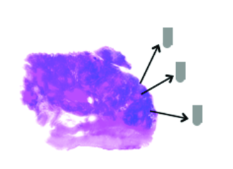
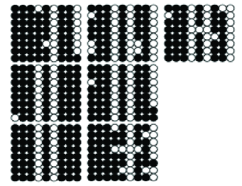
Figure 2.1: Left panel: sampling illustrated from three glands from one side of a colorectal tumour. Each gland contains 2,000–10,000 cells. Right panel: Methylation data from the BGN locus from 7 glands from the left side of Cancer 1 (CNC1, from [18]). 8 cells are sampled from each gland. Each row of 9 circles represents the methylation pattern in a cell. Solid circles denote methylated sites, open circles unmethylated. See Table 2.1 for further details.

Data obtained from methylation patterns may be compared in several ways. We focus on the simplest method that considers whether or not cells have the same allele (that is, an identical pattern of 0s and 1s). Here we do not exploit information about the detailed structure of the methylation patterns, for which the reader is referred to [18]. In Table 2.1 we present the data from Cancer 1 shown in Figure 2.1 in a different way. The body of the table shows the numbers of cells of each allele (or type) in each of the 7 samples. The third row of the Table shows the numbers $K_{i}$ of different alleles seen in each sample. In Table 2.2 we give a similar breakdown for data from the left side of Cancer 2.

The last column in Tables 2.1 and 2.2 gives the combined distribution of allelic variation at this locus in the two tumours. Qualitatively, the two tumours seem to have rather different behaviour: Cancer 1 has far fewer alleles than Cancer 2, and their allocation among the different samples is more homogeneous in Cancer 1 than in Cancer 2. In the next sections we develop some theory that allows us to analyse this variation more carefully.

Table 2.1: Data for Cancer 1. 13 alleles were observed in the 7 samples. Columns labelled 1–7 give the distribution of the alleles observed in each sample, and column 8 shows the combined data. Data from cancer CNC1 in [18].

$i$	1	2	3	4	5	6	7	8
$n_{i}$	8	8	8	8	8	8	8	56
$K_{i}$	4	2	1	3	3	5	5	13
$\hat{\theta}_{i}$	2.50	0.49	0.00	1.25	1.25	4.69	4.69	5.01
allele
1	1			5	5	1	4	16
2	5					3		8
3	1							1
4	1					1		2
5		7	8		2			17
6		1						1
7				2				2
8				1	1		1	3
9						2		2
10						1		1
11							1	1
12							1	1
13							1	1

Table 2.2: Data for Cancer 2. 27 alleles were observed in the 7 samples. Columns labelled 1–7 give the distribution of the alleles observed in each sample, and column 8 shows the combined data. Data from cancer COC1 in [18].

$i$	1	2	3	4	5	6	7	8
$n_{i}$	8	8	8	8	8	8	8	56
$K_{i}$	7	7	4	3	7	6	4	27
$\hat{\theta}_{i}$	23.11	23.11	2.50	1.25	23.11	9.23	2.50	19.88
allele
1	1							1
2	1							1
3	2	1	2	1				6
4	1							1
5	1	1						2
6	1							1
7	1							1
8		1	4	4		3		12
9		1						1
10		2						2
11		1						1
12		1						1
13			1			1		2
14			1					1
15				3				3
16					1			1
17					2		1	3
18					1			1
19					1		1	2
20					1			1
21					1			1
22					1			1
23						1		1
24						1		1
25						1	4	5
26						1		1
27							2	2

3 The Ewens sampling formula

Our focus is on identifying whether the data are consistent with a uniformly mixing collection of tumour cells that are in approximate stasis, or are more typical of patterns of growth such as described in Siegmund et al., [17, 18, 19]. Whatever the model, the basic ingredients that must be specified include how the cells are related, the details of which depend on the demographic model used to describe the tumour evolution, and the mutation process that describes the methylation patterns. A review is provided in Siegmund et al., [19]. We use a simple null model in which the population of cells is assumed to have evolved for some time with an approximately constant, large size of $N$ cells, the constancy of cell numbers mimicking stasis in tumour growth. The mutation model assumes that in each cell division there is probability $u$ of a mutation resulting in a type that has not been seen before—admittedly a crude approximation to the nature of methylation mutations arising in our sample. The mutations are assumed to be neutral, a reasonable assumption given that the BGN gene is expressed in connective tissue but not in the epithelium. Thus our model is a classical one from population genetics, the so-called infinitely-many-neutral-alleles model.

Under this model the distribution of the types observed in the combined data (i.e., the allele counts derived from the right-most columns of data from Tables 2.1 and 2.2) has a distribution that depends on the parameter $\theta=2Nu$. This distribution is known as the Ewens Sampling Formula [7], denoted by ESF($\theta)$, and may be described as follows. For a sample of $n$ cells, we write $(C_{1},C_{2},\ldots,C_{n})$ for the vector of counts given by

$$C_{j}=\mbox{number of types represented }j\mbox{ times in the sample},$$

where $C_{1}+2C_{2}+\cdots+nC_{n}=n$. For the Cancer 1 sample we have $n=56$ and

$$C_{1}=6,C_{2}=3,C_{3}=1,C_{8}=1,C_{16}=1,C_{17}=1,$$

whereas for Cancer 2 we also have $n=56$, but

$$C_{1}=17,C_{2}=5,C_{3}=2,C_{5}=1,C_{6}=1,C_{12}=1.$$

The distribution ESF($\theta$) is given by

$$\mbox{\bf P}[C_{1}=c_{1},\ldots,C_{n}=c_{n}]=\frac{n!}{\theta_{(n)}}\,\prod_{j=1}^{n}\left(\frac{\theta}{j}\right)^{c_{j}}\,\frac{1}{c_{j}!},$$ (3.1)

for $c_{1}+2c_{2}+\cdots+nc_{n}=n$ and $\theta_{(n)}:=\theta(\theta+1)\ldots(\theta+n-1)$. An explicit connection between mutations resulting in the ESF and the ancestral history of the individuals (cells) in the sample is provided by Kingman’s coalescent [13, 12], and the connection with the infinite population limit is given in Kingman, [11, 14].

We recall from [7] that $K=K_{n}:=C_{1}+\cdots+C_{n}$, the number of types in the sample, is a sufficient statistic for $\theta$, and that the maximum-likelihood estimator of $\theta$ is the solution of the equation

$$K_{n}=\mbox{\bf E}_{\theta}(K_{n})=\sum_{j=1}^{n}\frac{\theta}{\theta+j-1}.$$ (3.2)

The conditional distribution of the counts $C_{1}$, …, $C_{n}$ given $K_{n}$ does not depend on $\theta$, and thus may be used to assess the goodness-of-fit of the model.

1 The multi-observer ESF

So far, we have described the distribution of variation in the entire sample, rather than in each of the subsamples from the different glands separately. The joint law of the counts of different alleles seen in the $R$ glands (that is, by the $R$ observers) is precisely that obtained by taking a hypergeometric sample of sizes $n_{1}$, $n_{2}$, …, $n_{R}$ from the $n$ cells in the combined sample. It is a consequence of the consistency property of the ESF that the sample seen by each observer $i$ has its own ESF, with parameters $n_{i}$ and $\theta$, $i=1$, 2, …, $R$. Tables 2.1 and 2.2 give the observed values for the two tumour examples.

We are interested in assessing the goodness-of-fit of the tumour data subsamples to our simple model of a homogeneous tumour in stasis. Because $K_{n}$ is sufficient for $\theta$ in the combined sample, this can be performed by using the joint distribution of the counts seen by each observer, conditional on the value of $K_{n}$. To simulate from this distribution we use the Chinese Restaurant Process, as described in the next section.

2 The Chinese Restaurant Process

We use simulation to find the distribution of certain test statistics relating to the multiple observer data. To do this we exploit a simple way to simulate a sample of individuals (cells in our example) whose allele counts follow the ESF($\theta$). The method, known as the Chinese Restaurant Process (CRP), after Diaconis and Pitman, [6], simulates individuals in a sample sequentially. The first individual is given type 1. The second individual is either a new type (labelled 2) with probability $\theta/(\theta+1)$, or a copy of the type of individual 1, with probability $1/(\theta+1)$. Suppose that $k-1$ individuals have been assigned types. Individual $k$ is assigned a new type (the lowest unused positive integer) with probability $\theta/(\theta+k-1)$, or is assigned the type of one of individuals 1, 2, …, $k-1$ selected uniformly at random. Continuing until $k=n$ produces a sample of size $n$, and the joint distribution of the number of types represented once, twice, … is indeed ESF($\theta$).

Once the sample of $n$ individuals is generated, it is straightforward to subsample without replacement to obtain $R$ samples, of sizes $n_{1}$, …, $n_{R}$, in each of which the distribution of the allele counts follows the ESF($\theta$) of the appropriate size. This may be done sequentially, choosing $n_{1}$ without replacement to be the first sample, then $n_{2}$ from the remaining $n-n_{1}$ to form the second sample, and so on.

When samples of size $n$ are required to have a given number of alleles, say $K_{n}=k$, this is most easily arranged by the rejection method: the CRP is run to produce an $n$-sample, and that run is rejected unless the correct value of $k$ is observed. Since conditional on $K_{n}=k$ the distribution of the allele frequencies is independent of $\theta$, we have freedom to choose $\theta$, which may be taken as the MLE $\hat{\theta}$ determined in (3.2) to make the rejection probability as small as possible.

4 Analysis of the cancer data

We have noted that the combined data in the $R$-observer ESF have the ESF($\theta$) distribution with sample size $n=n_{1}+\cdots+n_{R}$, while the $i$th observer’s sample has ESF($\theta$) distribution with sample size $n_{i}$. Of course, these distributions are not independent. To test whether the combined data are consistent with the ESF, we may use a statistic suggested by Watterson, [23], based on the distribution of the sample homozygosity

$$F=\sum_{j=1}^{n}C_{j}\,\left(\frac{j}{n}\right)^{2}$$

found after conditioning on the number of types seen in the combined sample. Each marginal sample may be tested in a similar way using the appropriate value of $n$.

Since our cancer data arise as the result of a spatial sampling scheme, it is natural to consider statistics that are aimed at testing whether the samples can be assumed homogeneous, that is, are described by the multi-observer ESF. Knowing the answer to this question would aid in understanding the dynamics of tumour evolution, which in turn has implications for understanding metastasis and response to therapy.

To assess this, we use as a simple illustration the sample variance of the numbers of types seen in each sample. The statistic may be written as

$$Q\ :=\ \frac{1}{R-1}\,\sum_{i=1}^{R}(K_{i}-\bar{K})^{2}\ =\ \frac{1}{R(R-1)}\sum_{1\leq i<j\leq R}(K_{i}-K_{j})^{2},$$ (4.1)

the latter expression emphasizing its role as a measure of the average discrepancy between samples. In the next paragraphs, we discuss the structure of Cancers 1 and 2 using these statistics.

Cancer 1

We begin with a comparison of the data from the two sides of Cancer 1. In this case $n_{1}=56,n_{2}=56$ and the combined sample of $n=112$ has $K_{112}=16$ and $F=0.237$. The 5th and 95th percentiles of the null distribution of $F$ found by the conditional CRP simulation described in the last section are 0.108 and 0.277 respectively, suggesting no anomaly with the underlying ESF model. For the left side of the cancer (Table 2.1), $K_{56}=13$ and $F=0.209$, while for the right side (data not shown), $K_{56}=10$ and $F=0.293$. In both cases these observed values of $F$ are consistent with the ESF. We then use the statistic $Q$ to investigate whether the data from the 7 glands from the left side of the tumour are homogeneous. We observed $Q=2.24$, and the null distribution of $Q$ can also be found from the conditional CRP simulation. We obtained 5th and 95th percentiles of 0.29 and 2.48 respectively, supporting the conclusion of a homogeneous tumour.

Cancer 2

The comparison of the two sides of Cancer 2 is more interesting. Once more $n_{1}=56,n_{2}=56$ but the combined sample of $n=112$ now has $K_{112}=48$ and $F=0.081$. The 99th percentile of the null distribution of $F$ is 0.060, suggesting that the ESF model is not adequate to describe the combined data. At first glance the anomaly can be attributed to the data from the right side of the tumour (not shown here), for which $K_{56}=29$ and $F=0.105$, far exceeding the 99th percentile of 0.089. For the left side (Table 2.2), $F=0.083$, just below the 95th percentile of 0.084. Thus the left side seems in aggregate to be adequately described by the ESF model. Further examination of the data from the 7 glands reveals a different story. From the third row of Table 2.2 we calculate $Q=2.95$, far exceeding the estimated 99th percentile of 2.33. Thus a more detailed view of the way the mutations are shared among the glands shows that these data are indeed inconsistent with the homogeneity expected in the multi-observer ESF.

Of course, many other statistics could have been considered. A natural starting point for constructing them would be the numbers of alleles that are seen only by a specific subset $A$ of the observers, where $A$ ranges over the $2^{R}-2$ non-empty proper subsets of the $R$ observers. Such statistics form the basis of the results in Section 5.

Rejection of the null hypothesis of the uniformly mixing homogeneous tumour model can occur for many reasons, for example because of non-uniform mutation rates, different demography of cell growth, non-neutrality of the mutations (which might apply to the BGN locus if in fact it were expressed in tissue in the tumour), and unforeseen effects of the simple mutation model itself. Which of these hypotheses is most likely requires a far more detailed analysis of competing models, as for example outlined in [17, 18, 19].

5 Poisson approximation

In this section, we derive Poisson approximations to the joint distribution of the numbers of alleles that are seen only by specific subsets $A$ of the observers. As mentioned above, functionals of these counts can be used as statistics to test for the homogeneity of (subgroups of) observers. Our approximations come together with bounds on the total variation distance between the actual and approximate distributions. We begin with the case of $R=2$ observers, and with the statistic $K_{1}-K_{2}$.

1 2 observers

We write $C:=(C_{1},C_{2},\ldots)$, where $C_{j}=0$ for $j>n$, and recall Watterson’s result, that $(C_{1},\ldots,C_{n})$ are jointly distributed according to ${\cal L}(Z_{1},Z_{2},\ldots,Z_{n}\,|\,T_{0n}(Z)=n)$, where $(Z_{j},\,j\geq 1)$ are independent with $Z_{i}\sim{\rm Po}\,(\theta/i)$, and

$$T_{rs}(c)\ =\ \sum_{j=r+1}^{s}jc_{j},\qquad c\in\mathbb{Z}_{+}^{\infty},$$ (5.1)

[22]. The sampled individuals can be labelled 1 or 2, according to which observer sampled them; under the above model, the $n_{1}$ 1-labels and $n_{2}$ 2-labels are distributed at random among the individuals, irrespective of their allelic type. Let $K_{r}$ denote the number of distinct alleles observed by the $r$-th observer, $r=1$, 2. Ewens et al., [8] observed that, in the case $n_{1}=n_{2}$ and for large $n$, $(K_{1}-K_{2})/\log n$ is equivalent to the difference in the estimates of the mutation rate made by the two observers. The same is asymptotically true also as $n$ becomes large, if $n_{1}/n\sim p_{1}$ for any fixed $p_{1}$. This motivates us to look for a distributional approximation to the distribution of the difference $K_{1}-K_{2}$.

Theorem 5.1.

For any $n_{1}$, $n_{2}$ and $b$,

$$d_{\mbox{\tiny TV}}({\cal L}(K_{1}-K_{2}),{\cal L}(P_{1}-P_{2}))\ \leq\ \frac{kb}{n-1}+\frac{k^{\prime}\rho^{b+1}}{(b+1)(1-\rho)},$$

for suitable constants $k$ and $k^{\prime}$, where $P_{1}$ and $P_{2}$ are independent Poisson random variables having means $\theta\log\{1/(1-p_{1})\}$ and $\theta\log\{1/(1-p_{2})\}$ respectively, with $p_{r}:=n_{r}/n$, and where $\rho=\max\{1-p_{1},1-p_{2}\}$. The choice $b=b_{n}=\lfloor\log n/\log(1/\rho)\rfloor$ gives a bound of order $O\bigl{(}\log n/(n\min\{p_{1},p_{2}\})\bigr{)}$.

Proof.

Group the individuals in the combined sample according to their allelic type, and let $M_{js}$ denote the number of individuals that were observed by observer 1 in the $s$-th of the $C_{j}$ groups of size $j$, the remaining $j-M_{js}$ being observed by observer 2. Define

$$S_{j}^{1}\ :=\ \sum_{s=1}^{C_{j}}I[M_{js}=j]\quad\mbox{and}\quad S_{j}^{2}\ :=\ \sum_{s=1}^{C_{j}}I[M_{js}=0]$$

to be the numbers of $j$-groups observed only by observers 1 and 2, respectively. Then it follows that

$$K_{1}-K_{2}\ =\ S^{1}-S^{2},$$

where $S^{r}:=\sum_{j=1}^{n}S_{j}^{r}$ . The first step in the proof is to show that the effect of the large groups is relatively small.

Note that the probability that an allele which is present $j$ times in the combined sample was not observed by observer 1 is

$$\prod_{i=0}^{j-1}\frac{n_{1}-i}{n-i}\ \leq\ (1-p_{1})^{j};$$

similarly, the probability that it was not observed by observer 2 is at most $(1-p_{2})^{j}$. Hence, conditional on $C$, the probability that any of the alleles present more than $b$ times in the combined sample is seen by only one of the observers is at most

$$\mbox{\bf E}\Biggl{\{}\,\sum_{j=b+1}^{n}(S_{j}^{1}+S_{j}^{2})\,\Bigg{|}\,C\Biggr{\}} \ \leq\ \sum_{j=b+1}^{n}C_{j}\{(1-p_{1})^{j}+(1-p_{2})^{j}\}$$

$$\ \leq\ 2\sum_{j=b+1}^{n}\rho^{j}C_{j},$$

whatever the value of $b$. Hence, writing $U_{b}:=\sum_{j=1}^{b}(S_{j}^{1}-S_{j}^{2})$, we find that

$$\mbox{\bf P}[K_{1}-K_{2}\neq U_{b}]\ \leq\ 2\sum_{j=b+1}^{n}\rho^{j}\mbox{\bf E}C_{j}\ \leq\ \frac{2k_{1}\rho^{b+1}}{(b+1)(1-\rho)},$$ (5.2)

where, by Watterson’s formula [22] for the means of the component sizes, we can take $k_{1}:=(2\theta+e^{-1})$ if $n\geq 4(b+1)$ (and $k_{1}:=\theta$ if $\theta\geq 1$).

To approximate the distribution of $U_{b}$, note that, conditional on $C$, the number of 1-labels among the individuals in allele groups of at most $b$ individuals has a hypergeometric distribution

$${\rm HG}\,(T_{0b}(C);n_{1};n),$$

where ${\rm HG}\,(s;m;n)$ denotes the number of black balls obtained in $s$ draws from an urn containing $m$ black balls out of a total of $n$. By Theorem 3.1 of Holmes, [10], we have

$$d_{\mbox{\tiny TV}}({\rm HG}\,(T_{0b}(C);n_{1};n),{\rm Bi}\,(T_{0b}(C),p_{1}))\ \leq\ \frac{T_{0b}(C)-1}{n-1}.$$ (5.3)

Hence, conditional on $C$, the joint distribution of labels among individuals differs in total variation from that obtained by independent Bernoulli random assignments, with label 1 having probability $p_{1}$ and label 2 probability $p_{2}$, by at most $(T_{0b}(C)-1)/(n-1)$.

Now, by Lemma 5.3 of Arratia et al., [2], we also have

$$d_{\mbox{\tiny TV}}({\cal L}(C_{1},\ldots,C_{b}),{\cal L}(Z_{1},\ldots,Z_{b}))\ \leq\ \frac{c_{\theta}b}{n},$$

with $c_{\theta}\leq 4\theta(\theta+1)/3$ if $n\geq 4b$. Hence, and from (5.3), it follows that

$$d_{\mbox{\tiny TV}}({\cal L}(C_{1},\ldots,C_{b};\{M_{js},\,1\leq s\leq C_{j},\,1\leq j\leq b\}),$$

$$\qquad\qquad\qquad{\cal L}(Z_{1},\ldots,Z_{b};\{N_{js},\,1\leq s\leq Z_{j},\,1\leq j\leq b\}))$$

$$\qquad\ \leq\ \frac{c_{\theta}b}{n}+\frac{\mbox{\bf E}(T_{0b}(C))-1}{n-1},$$ (5.4)

where $(N_{js};\,s\geq 1,\,1\leq j\leq b)$ are independent of each other and of $Z_{1}$, …, $Z_{b}$, with $N_{js}\sim{\rm Bi}\,(j,p)$. But now the values of the $N_{js}$, $1\leq s\leq Z_{j}$, $1\leq j\leq b$, can be interpreted as the numbers of 1-labels assigned to each of $Z_{j}$ groups of size $j$ for each $1\leq j\leq b$, again under independent Bernoulli random assignments, with label 1 having probability $p_{1}$ and label 2 probability $p_{2}$. Hence, since the $Z_{j}$ are independent Poisson random variables, the counts

$$T_{j}^{1}\ :=\ \sum_{s=1}^{Z_{j}}I[N_{js}=j]\quad\mbox{and}\quad T_{j}^{2}\ :=\ \sum_{s=1}^{Z_{j}}I[N_{js}=0]$$

are pairs of independent Poisson distributed random variables, with means $\theta j^{-1}p_{1}^{j}$ and $\theta j^{-1}p_{2}^{j}$, and are also independent of one another. Hence it follows that

$$V_{b}\ :=\ \sum_{j=1}^{b}(T_{j}^{1}-T_{j}^{2})\ \sim\ P_{1b}-P_{2b},$$ (5.5)

where $P_{1b}$ and $P_{2b}$ are independent Poisson random variables, with means $\theta\sum_{j=1}^{b}j^{-1}p_{1}^{j}$ and $\theta\sum_{j=1}^{b}j^{-1}p_{2}^{j}$, respectively. Comparing the definitions of $U_{b}$ and $V_{b}$, and combining (5.4) and (5.5), it thus follows that

$$d_{\mbox{\tiny TV}}({\cal L}(U_{b}),{\cal L}(P_{1b}-P_{2b}))\ \leq\ \frac{(c_{\theta}+k_{2})b}{n-1},$$ (5.6)

with $k_{2}=4\theta/3$ for $n\geq 4b$, once again by Watterson’s formula [22].

With (5.2) and (5.6), the argument is all but complete; it simply suffices to observe that, much as in proving (5.2),

$$d_{\mbox{\tiny TV}}({\cal L}(P_{1}),{\cal L}(P_{1b}))+d_{\mbox{\tiny TV}}({\cal L}(P_{2}),{\cal L}(P_{2b}))\ \leq\ \frac{2\theta\rho^{b+1}}{(b+1)(1-\rho)};$$

we take $k:=4\vee(c_{\theta}+k_{2})$ and $k^{\prime}:=2(\theta+k_{1})$. ∎

2 $R$ observers

The proof of Theorem 5.1 actually shows that the joint distribution of $S^{1}$ and $S^{2}$, the numbers of types seen respectively by observers 1 and 2 alone, is close to that of independent Poisson random variables $P_{1}$ and $P_{2}$. For $R\geq 3$ observers, we use a similar approach to derive an approximation to the joint distribution of the numbers of alleles seen by each proper subset $A$ of the $R$ observers.

Suppose that the $r$-th observer samples $n_{r}$ individuals, $1\leq r\leq R$, and set $n:=\sum_{r=1}^{R}n_{r}$, $p_{r}:=n_{r}/n$. Define the component frequencies in the combined sample as before, and set $M_{js}=m:=(m_{1},\ldots,m_{R})$ if the $r$-th observer sees $m_{r}$ of the $j$ individuals in the $s$-th of the $C_{j}$ groups of size $j$. For any ${\emptyset\neq A\subsetneq[R]}$, where $[R]:=\{1,2,\ldots,R\}$, define

$${\mathcal{M}}_{Aj}\ :=\$$

$${}\quad\Bigl{\{}m\in\mathbb{Z}_{+}^{R}\colon\,\sum_{r=1}^{R}m_{r}=j,\,\{r\colon\,m_{r}\geq 1\}=A,\,\{r\colon\,m_{r}=0\}=[R]\setminus A\Bigr{\}},$$

and set

$$S_{j}^{A}\ :=\ \sum_{s=1}^{C_{j}}I[M_{js}\in A].$$

Our interest lies now in approximating the joint distribution of the counts $(S^{A},\allowbreak{\emptyset\neq A\subsetneq[R]})$, where $S^{A}:=\sum_{j=1}^{n}S_{j}^{A}$. To do so, we need a set of independent Poisson random variables $(P^{A},\,{\emptyset\neq A\subsetneq[R]})$, with $P^{A}\sim{\rm Po}\,(\lambda^{A}(\theta))$, where

$$\lambda_{j}^{A}(\theta)\ :=\ \frac{\theta}{j}\,{\rm MN}\,(j;p_{1},\ldots,p_{R})\{{\mathcal{M}}_{Aj}\}\quad\mbox{and}\quad\lambda^{A}(\theta)\ :=\ \sum_{j\geq 1}\lambda_{j}^{A}(\theta);$$ (5.7)

here, ${\rm MN}\,(j;p_{1},\ldots,p_{R})$ denotes the multinomial distribution with $j$ trials and cell probabilities $p_{1}$, …, $p_{R}$.

Theorem 5.2.

In the above setting, we have

$$d_{\mbox{\tiny TV}}\Bigl{(}{\cal L}((S^{A},\,{\emptyset\neq A\subsetneq[R]})),\mathop{\raisebox{-2.15277pt}{\hbox{\huge{$\times$}}}}_{{\emptyset\neq A\subsetneq[R]}}{\rm Po}\,(\lambda^{A}(\theta))\Bigr{)}$$

$${}\qquad\ \leq\ \frac{k_{R}b}{n}+\frac{k_{R}^{\prime}\rho^{b+1}}{(b+1)(1-\rho)},$$

where $\rho:=\max_{1\leq r\leq R}(1-p_{r})$. Again $b=b_{n}=\lfloor\log n/\log(1/\rho)\rfloor$ is a good choice.

Proof.

The proof runs much as before. First, the bound

$$\mbox{\bf E}\Biggl{\{}\sum_{j=b+1}^{n}\sum_{{\emptyset\neq A\subsetneq[R]}}S_{j}^{A}\,\Bigg{|}\,C\Biggr{\}}\ \leq\ \sum_{j=b+1}^{n}C_{j}\sum_{r=1}^{R}(1-p_{r})^{j}\ \leq\ R\sum_{j=b+1}^{n}\rho^{j}C_{j}$$

shows that

$$\mbox{\bf P}\left[\bigcup_{{\emptyset\neq A\subsetneq[R]}}\{S^{A}\neq S^{A}_{(b)}\}\right]\ \leq\ \frac{Rk_{1}\rho^{b+1}}{(b+1)(1-\rho)},$$ (5.8)

where $S^{A}_{(b)}:=\sum_{j=1}^{b}S_{j}^{A}$. Then, by Theorem 4 of Diaconis and Freedman, [5],

$$d_{\mbox{\tiny TV}}\Bigl{(}{\rm HG}\,(T_{0b}(C);n_{1},\ldots,n_{R};n),{\rm MN}\,(T_{0b}(C);p_{1},\ldots,p_{R})\Bigr{)}\ \leq\ \frac{RT_{0b}}{n},$$

from which it follows that

$$d_{\mbox{\tiny TV}}\Bigl{(}{\cal L}(C_{1},\ldots,C_{b};\{M_{js},\,1\leq s\leq C_{j},\,1\leq j\leq b\}),$$

$$\qquad\qquad\qquad{\cal L}(Z_{1},\ldots,Z_{b};\{N_{js},\,1\leq s\leq Z_{j},\,1\leq j\leq b\})\Bigr{)}$$

$$\qquad\ \leq\ \frac{c_{\theta}b}{n}+\frac{R\mbox{\bf E}(T_{0b}(C))}{n},$$ (5.9)

where $(N_{js};\,s\geq 1,\,1\leq j\leq b)$ are independent of each other and of $Z_{1}$, …, $Z_{b}$, with $N_{js}\sim{\rm MN}\,(j;p_{1},\ldots,p_{R})$. Then the random variables

$$T_{j}^{A}\ :=\ \sum_{s=1}^{Z_{j}}I[N_{js}\in A],\qquad{\emptyset\neq A\subsetneq[R]},$$

are independent and Poisson distributed, with means $\lambda^{A}_{(b)}(\theta):=\break\sum_{j=1}^{b}\lambda_{j}^{A}(\theta)$, and

$$d_{\mbox{\tiny TV}}\{{\cal L}(S^{A}_{(b)},\,{\emptyset\neq A\subsetneq[R]}),\,{\cal L}(T^{A}_{(b)},\,{\emptyset\neq A\subsetneq[R]})\}\ \leq\ \frac{k_{2}^{\prime}b}{n},$$

with $k_{2}^{\prime}:=c_{\theta}+4R\theta/3$, where

$$T^{A}_{(b)}\ :=\ \sum_{j=1}^{b}T^{A}_{j}\ \sim\ {\rm Po}\,(\lambda^{A}_{(b)}(\theta)).$$

Finally, much as before,

$$d_{\mbox{\tiny TV}}\Bigl{(}{\cal L}((T^{A}_{(b)},\,{\emptyset\neq A\subsetneq[R]})),\,\mathop{\raisebox{-2.15277pt}{\hbox{\huge{$\times$}}}}_{{\emptyset\neq A\subsetneq[R]}}{\rm Po}\,(\lambda^{A}(\theta))\Bigr{)}\ \leq\ \frac{R\theta\rho^{b+1}}{(b+1)(1-\rho)},$$

and we can take $k_{R}:=4\vee(c_{\theta}+Rk_{2})$ and $k_{R}^{\prime}:=R(\theta+k_{1})$ in the theorem. ∎

We note that the Poisson means $\lambda_{j}^{A}(\theta)$ appearing in (5.7) may be calculated using an inclusion-exclusion argument. For reasons of symmetry it is only necessary to compute $\lambda_{j}^{A}(\theta)$ for sets of the form $A=[r]=\{1,2,\ldots,r\}$ for $r=1$, 2, …, $R-1$. We obtain

$${\rm MN}(j;p_{1},\ldots,p_{R})\{{\mathcal{M}}_{[r]j}\}=\sum_{l=1}^{r}(-1)^{r-l}\sum_{J\subseteq[r],|J|=l}\left(\sum_{u\in J}p_{u}\right)^{j},$$ (5.10)

from which the terms $\lambda^{A}(\theta)$ readily follow as

$$\lambda^{[r]}(\theta)=-\theta\,\sum_{l=1}^{r}(-1)^{r-l}\sum_{J\subseteq[r],|J|=l}\log\left(1-\sum_{u\in J}p_{u}\right).$$ (5.11)

3 The conditional distribution

In statistical applications, such as that discussed above, the value of $\theta$ is unknown, and has to be estimated. Defining

$$K_{st}(c)\ :=\ \sum_{j=s+1}^{t}c_{j},$$

the quantity $K_{0n}(C)$ is sufficient for $\theta$, and the null distribution appropriate for testing model fit is then the conditional distribution

$${\cal L}((S^{A},\,{\emptyset\neq A\subsetneq[R]})\,|\,K_{0n}(C)=k),$$

where $k$ is the observed value of $K_{0n}(C)$. Hence we need to approximate this distribution as well. Because of sufficiency, the distribution no longer involves $\theta$. However, for our approximation, we shall need to define means for the approximating Poisson random variables $P^{A}\sim{\rm Po}\,(\lambda^{A}(\theta))$, as in (5.7), and these need a value of $\theta$ for their definition. We thus take $\lambda^{A}(\theta_{k})$ for our approximation, for convenience with $\theta_{k}:=k/\log n$; the MLE given in (3.2) could equally well have been used.

The proof again runs along the same lines. Supposing that the probabilities $p_{1}$, …, $p_{R}$ are bounded away from $0$, we can take $b:=b_{n}:=\lfloor\log n/\log(1/\rho)\rfloor$ in Theorem 5.2, and use (5.8) to show that it is enough to approximate ${\cal L}((S^{A}_{(b)},\,{\emptyset\neq A\subsetneq[R]})\,|\,K_{0n}(C)=k)$. Then, since the arguments conditional on the whole realization $C$ remain the same when restricting $C$ to the set $\{K_{0n}(C)=k\}$, it is enough to show that the distributions

$${\cal L}(C_{[0,b]}\,|\,K_{0n}(C)=k)\quad\mbox{and}\quad{\cal L}_{\theta_{k}}(Z_{[0,b]})$$

are close enough, where $c_{[0,b]}:=(c_{1},\ldots,c_{b})$, to conclude that the Poisson approximation of Theorem 5.2 with $\theta=\theta_{k}$ also holds conditionally on $\{K_{0n}(C)=k\}$. Note also that the event $\{K_{0n}(C)=k\}$ has probability at least as big as $c_{1}(\theta_{k})k^{-1/2}$ for some positive function $c_{1}(\cdot)$, by (8.17) of Arratia et al., [2].

Defining $\lambda_{st}(\theta_{k}):=\sum_{j=s+1}^{t}j^{-1}\theta_{k}$, we can now prove the key lemma.

Lemma 5.3.

Fix any $\varepsilon,\eta>0$. Suppose that $n$ is large enough, so that $b+b^{3}<n/2$. Then there is a constant $\kappa$ such that, uniformly for $\varepsilon\leq k/\log n\leq 1/\varepsilon$, and for $c\in\mathbb{Z}_{+}^{\infty}$ with $K_{0b}(c)\leq\eta\log\log n$ and $T_{0b}(c)\leq b^{7/2}$,

$$\left|\frac{\mbox{\bf P}[C_{[0,b]}=c_{[0,b]}\,|\,K_{0n}(C)=k]}{\mbox{\bf P}_{\theta_{k}}[Z_{[0,b]}=C_{[0,b]}]}-1\right|\ \leq\ \frac{\kappa\log\log n}{\log n}.$$

Proof.

Since ${\cal L}(C_{1},\ldots,C_{n})={\cal L}(Z_{1},\ldots,Z_{n}\,|\,T_{0n}(Z)=n)$, it follows that

$$\mbox{\bf P}[C_{[0,b]}=c_{[0,b]}\,|\,K_{0n}(C)=k]$$

$$= \frac{\mbox{\bf P}[K_{0n}(C)=k\,|\,C_{[0,b]}=c_{[0,b]}]\mbox{\bf P}[C_{[0,b]}=c_{[0,b]}]}{\mbox{\bf P}[K_{0n}(C)=k]}$$

$$= \frac{\mbox{\bf P}[K_{bn}(C)=k-K_{0b}(c)\,|\,T_{0b}(C)=T_{0b}(c)]\mbox{\bf P}[C_{[0,b]}=c_{[0,b]}]}{\mbox{\bf P}[K_{0n}(C)=k]}.$$

We now use results from §13.10 of Arratia et al., [2]. First, as on p. 323,

$$\mbox{\bf P}_{\theta_{k}}[K_{bn}(C)=k-K_{0b}(c)\,|\,T_{0b}(C)=T_{0b}(c)]$$

$$= \mbox{\bf P}_{\theta_{k}}[K_{bn}(Z)=k-K_{0b}(c)\,|\,T_{bn}(Z)=n-T_{0b}(c)],$$

and the estimate on p. 327 then gives

$$\mbox{\bf P}_{\theta_{k}}[K_{bn}(Z)=k-K_{0b}(c)\,|\,T_{bn}(Z)=n-T_{0b}(c)]$$ (5.12)

$$= {\rm Po}\,(\lambda_{bn}(\theta_{k}))\{k-K_{0b}(c)-1\}\,\{1+O((\log n)^{-1}\log\log n)\},\phantom{X}$$

uniformly in the chosen ranges of $k$, $T_{0b}(c)$ and $K_{0b}(c)$, because of the choice $\theta=\theta_{k}$. Then

$$\mbox{\bf P}_{\theta_{k}}[K_{0n}(C)=k]\ =\ {\rm Po}\,(\lambda_{0n}(\theta_{k}))\{k-1\}\,\{1+O((\log n)^{-1})\},$$ (5.13)

again uniformly in $k$, $T_{0b}(c)$ and $K_{0b}(c)$, by Theorem 5.4 of Arratia et al., [1]. Finally,

$$\left|\frac{\mbox{\bf P}_{\theta_{k}}[C_{[0,b]}=c_{[0,b]}]}{\mbox{\bf P}_{\theta_{k}}[Z_{[0,b]}=c_{[0,b]}]}-1\right| \ =\ \left|\frac{\mbox{\bf P}_{\theta_{k}}[T_{bn}(Z)=n-T_{0b}(c)]}{\mbox{\bf P}_{\theta_{k}}[T_{bn}(Z)=n]}-1\right|$$

$$\ =\ O(n^{-1}b^{7/2}),$$

by (4.43), (4.45) and Example 9.4 of [2], if $b+b^{3}<n/2$. The lemma now follows by considering the ratio of the Poisson probabilities in (5.12) and (5.13); note that $\lambda_{0n}(\theta_{k})-\lambda_{bn}(\theta_{k})=O(\log\log n)$. ∎

In order to deduce the main theorem of this section, we just need to bound the conditional probabilities of the events $\{K_{0b}(C)>\eta\log\log n\}$ and $\{T_{0b}(C)>b^{7/2}\}$, given $K_{0n}(C)=k$. For the first, note that

$$\mbox{\bf P}_{\theta_{k}}[K_{0b}(C)>\eta\log\log n]\ \leq\ \frac{c_{\theta_{k}}b}{n}+\mbox{\bf P}_{\theta_{k}}[K_{0b}(Z)>\eta\log\log n],$$ (5.14)

and that $K_{0b}(Z)\sim{\rm Po}\,(\theta_{k}\sum_{j=1}^{b}j^{-1})$ with mean of order $O(\log\log n)$. Hence there is an $\eta$ large enough that

$$\mbox{\bf P}_{\theta_{k}}[K_{0b}(C)>\eta\log\log n]\ =\ O((\log n)^{-5/2}),$$

uniformly in the given range of $k$. Since also, from (5.13),

$$\mbox{\bf P}_{\theta_{k}}[K_{0n}(C)=k]\ \geq\ \eta^{\prime}/\sqrt{\log n}$$

for some $\eta^{\prime}>0$, it follows immediately that

$$\mbox{\bf P}_{\theta_{k}}[K_{0b}(C)>\eta\log\log n\,|\,K_{0n}(C)=k]\ =\ O((\log n)^{-2}).$$ (5.15)

The second inequality is similar. We use the argument of (5.14) to reduce consideration to $\mbox{\bf P}_{\theta_{k}}[T_{0b}(Z)>b^{7/2}]$, and (4.44) of Arratia et al., [2] shows that

$$\mbox{\bf P}_{\theta_{k}}[T_{0b}(Z)>b^{7/2}]\ =\ O(b^{-5/2})\ =\ O((\log n)^{-5/2});$$

the conclusion is now as for (5.15).

In view of these considerations, we have established the following theorem, justifying the Poisson approximation to the conditional distribution of the $(S^{A},\,{\emptyset\neq A\subsetneq[R]})$, using the estimated value $\theta_{k}$ of $\theta$ as parameter.

Theorem 5.4.

For any $0<\varepsilon<1$, uniformly in $\varepsilon\leq k/\log n\leq 1/\varepsilon$, we have

$$d_{\mbox{\tiny TV}}\Bigl{(}{\cal L}((S^{A},\,{\emptyset\neq A\subsetneq[R]})\,|\,K_{0n}(C)=k),\mathop{\raisebox{-2.15277pt}{\hbox{\huge{$\times$}}}}_{{\emptyset\neq A\subsetneq[R]}}{\rm Po}\,(\lambda^{A}(\theta_{k}))\Bigr{)}$$

$${}\qquad\ =\ O\Bigl{(}\frac{\log\log n}{\log n}\Bigr{)}.$$

Note that the error bound is much larger for this approximation than those in the previous theorems. However, it is not unreasonable. From (5.8), the joint distribution of the $S^{A}$ is almost entirely determined by that of $C_{1}$, …, $C_{b}$. Now ${\cal L}(K_{0b}(C)\,|\,K_{0n}(C)=k)$ can be expected to be close to ${\cal L}(K_{0b}(Z)\,|\,K_{0n}(Z)=k)$, which is binomial ${\rm Bi}\,(k,p_{b,n})$, where

$$p_{b,n}\ :=\ \frac{\sum_{j=1}^{b}1/j}{\sum_{j=1}^{n}1/j}\ \approx\ \frac{\log b}{\log n}\ \approx\ \frac{\log\log n}{\log(1/\rho)\log n}.$$

On the other hand, from Lemma 5.3 of [2], the unconditional distribution of $K_{0b}(C)$ is very close to that of $K_{0b}(Z)$, a Poisson distribution. The total variation distance between the distributions ${\rm Po}\,(kp)$ and ${\rm Bi}\,(k,p)$ is of exact order $p$ if $kp$ is large (Theorem 2 of Barbour and Hall, [3]). Since $p_{b,n}\asymp\log\log n/\log n$, an error of this order in Theorem 5.4 is thus in no way surprising.

We can now compute the mean $\mu$ of the approximation to the distribution of $Q$, as used in Section 4, obtained by using Theorem 5.4. We begin by noting that, using the theorem,

$$K_{r}-K_{s}\ =\ \sum_{A\colon\,r\in A,s\notin A}S^{A}-\sum_{A\colon\,r\notin A,s\in A}S^{A}$$

is close in distribution to

$${\widehat{K}}_{rs}-{\widehat{K}}_{sr}\ :=\ \sum_{A\colon\,r\in A,s\notin A}P^{A}-\sum_{A\colon\,r\notin A,s\in A}P^{A},$$

where $P^{A}\sim{\rm Po}\,(\lambda^{A}(\theta_{k}))$, ${\emptyset\neq A\subsetneq[R]}$, are independent. To compute the means

$$\lambda_{rs}\ :=\ \sum_{A\colon\,r\in A,s\notin A}\lambda^{A}(\theta_{k})\quad\mbox{and}\quad\lambda_{sr}\ :=\ \sum_{A\colon\,r\notin A,s\in A}\lambda^{A}(\theta_{k})$$

of ${\widehat{K}}_{rs}$ and ${\widehat{K}}_{sr}$, we note that

$$\sum_{A\colon\,r\in A,s\notin A}{\rm MN}\,(j;p_{1},\ldots,p_{R})\{{\mathcal{M}}_{Aj}\}$$

$${}\qquad=(1-p_{s})^{j}\{1-(1-p_{r}/(1-p_{s}))^{j}\}$$

$${}\qquad=(1-p_{s})^{j}-(1-p_{r}-p_{s})^{j},$$

the probability under the multinomial scheme that the $r$-th cell is non-empty but the $s$-th cell is empty. Thus

$$\lambda_{rs}\ =\ \sum_{j\geq 1}\frac{\theta_{k}}{j}\,\{(1-p_{s})^{j}-(1-p_{r}-p_{s})^{j}\}\ =\ \theta_{k}\log((p_{r}+p_{s})/p_{s}),$$

and $\lambda_{sr}=\theta_{k}\log((p_{r}+p_{s})/p_{r})$. Then, because ${\widehat{K}}_{rs}$ and ${\widehat{K}}_{sr}$ are independent and Poisson distributed,

$$\mbox{\bf E}\{({\widehat{K}}_{rs}-{\widehat{K}}_{sr})^{2}\}\ =\ (\lambda_{rs}-\lambda_{sr})^{2}+\lambda_{rs}+\lambda_{sr}.$$

This yields the formula

$$\mu\ :=\ \frac{1}{R(R-1)}\,\sum_{1\leq r<s\leq R}\left\{\theta_{k}^{2}\{\log(p_{r}/p_{s})\}^{2}+\theta_{k}\log\left(\frac{(p_{r}+p_{s})^{2}}{p_{r}p_{s}}\right)\right\}.$$ (5.16)

In particular, if $p_{r}=1/R$ for $1\leq r\leq R$, then $\mu=\theta_{k}\log 2$, agreeing with the observation of Ewens et al., [8] in the case $R=2$.

6 Conclusion

Our paper is about ancestral inference (albeit in a somatic cell setting rather than the typical population genetics one) and Poisson approximation. John Kingman has made fundamental and far-reaching contributions to both areas. It therefore gives us great pleasure to dedicate it to John on his birthday.

Acknowledgements

ST acknowledges the support of the University of Cambridge, Cancer Research UK and Hutchison Whampoa Limited. ADB was supported in part by Schweizer Nationalfonds Projekt Nr. 20–117625/1.

References

- Arratia et al., [2000] Arratia, R., Barbour, A. D., and Tavaré, S. 2000. The number of components in a logarithmic combinatorial structure. Ann. Appl. Probab., 10, 331–361.
- Arratia et al., [2003] Arratia, R., Barbour, A. D., and Tavaré, S. 2003. Logarithmic Combinatorial Structures: A Probabilistic Approach. EMS Monogr. Math., vol. 1. Zürich: Eur. Math. Soc.
- Barbour and Hall, [1984] Barbour, A. D., and Hall, P. G. 1984. On the rate of Poisson convergence. Math. Proc. Cambridge Philos. Soc., 95, 473–480.
- Campbell et al., [2008] Campbell, P. J., Pleasance, E. D., Stephens, P. J., Dicks, E., Rance, R., Goodhead, I., Follows, G. A., Green, A. R., Futreal, P. A., and Stratton, M. R. 2008. Subclonal phylogenetic structures in cancer revealed by ultra-deep sequencing. Proc. Natl. Acad. Sci. USA, 105, 13081–13086.
- Diaconis and Freedman, [1980] Diaconis, P., and Freedman, D. 1980. Finite exchangeable sequences. Ann. Probab., 8, 745–764.
- Diaconis and Pitman, [1986] Diaconis, P., and Pitman, J. 1986. Permutations, Record Values and Random Measures. Unpublished lecture notes, Statistics Department, University of California, Berkeley.
- Ewens, [1972] Ewens, W. J. 1972. The sampling theory of selectively neutral alleles. Theor. Population Biology, 3, 87–112.
- Ewens et al., [2007] Ewens, W. J., RoyChoudhury, A., Lewontin, R. C., and Wiuf, C. 2007. Two variance results in population genetics theory. Math. Popul. Stud., 14, 1–18.
- Greenman et al., [2006] Greenman, C., Wooster, R., Futreal, P. A., Stratton, M. R., and Easton, D. F. 2006. Statistical analysis of pathogenicity of somatic mutations in cancer. Genetics, 173, 2187–2198.
- Holmes, [2004] Holmes, S. 2004. Stein’s method for birth and death chains. Pages 45–67 of: Diaconis, P., and Holmes, S. (eds), Stein’s Method: Expository Lectures and Applications. IMS Lecture Notes Monogr. Ser., vol. 46. Beachwood, OH: Inst. Math. Statist.
- Kingman, [1982a] Kingman, J. F. C. 1982a. The coalescent. Stochastic Process. Appl., 13, 235–248.
- Kingman, [1982b] Kingman, J. F. C. 1982b. Exchangeability and the evolution of large populations. Pages 97–112 of: Koch, G., and Spizzichino, F. (eds), Exchangeability in Probability and Statistics. Amsterdam: North-Holland.
- Kingman, [1982c] Kingman, J. F. C. 1982c. On the genealogy of large populations. J. Appl. Probab., 19A, 27–43.
- Kingman, [1993] Kingman, J. F. C. 1993. Poisson Processes. Oxford Studies in Probability, vol. 3. Oxford: Oxford University Press.
- Merlo et al., [2006] Merlo, L. M. F., Pepper, J. W., Reid, B. J., and Maley, C. C. 2006. Cancer as an evolutionary and ecological process. Nature Reviews Cancer, 6, 924–935.
- Shah et al., [2009] Shah, S. P., Morin, R. D., Khattra, J., Prentice, L., Pugh, T., Burleigh, A., Delaney, A., Gelmon, K., Guliany, R., Senz, J., Steidl, C., Holt, R. A., Jones, S., Sun, M., Leung, G., Moore, R., Severson, T., Taylor, G. A., Teschendorff, A. E., Tse, K., Turashvili, G., Varhol, R., Warren, R. L., Watson, P., Zhao, Y., Caldas, C., Huntsman, D., Hirst, M., Marra, M. A., and Aparicio, S. 2009. Mutational evolution in a lobular breast tumour profiled at single nucleotide resolution. Nature, 461, 809–813.
- Siegmund et al., [2008] Siegmund, K. D., Marjoram, P., and Shibata, D. 2008. Modeling DNA methylation in a population of cancer cells. Stat. Appl. Genet. Mol. Biol., 7, Article 18.
- Siegmund et al., [2009a] Siegmund, K. D., Marjoram, P., Woo, Y-J., Tavaré, S., and Shibata, D. 2009a. Inferring clonal expansion and cancer stem cell dynamics from dna methylation patterns in colorectal cancers. Proc. Natl. Acad. Sci. USA, 106, 4828–4833.
- Siegmund et al., [2009b] Siegmund, K. D., Marjoram, P., Tavaré, S., and Shibata, D. 2009b. Many colorectal cancers are “flat” clonal expansions. Cell Cycle, 8, 2187–2193.
- Sjöblom et al., [2006] Sjöblom, T., Jones, S., Wood, L. D., Parsons, D. W., Lin, J., Barber, T. D., Mandelker, D., Leary, R. J., Ptak, J., Silliman, N., Szabo, S., Buckhaults, P., Farrell, C., Meeh, P., Markowitz, S. D., Willis, J., Dawson, D., Willson, J. K. V., Gazdar, A. F., Hartigan, J., Wu, L., Liu, C., Parmigiani, G., Park, B. H., Bachman, K. E., Papadopoulos, N., Vogelstein, B., Kinzler, K. W., and Velculescu, V. E. 2006. The consensus coding sequences of human breast and colorectal cancers. Science, 314, 268–274.
- Tsao et al., [2000] Tsao, J. L., Yatabe, Y., Salovaara, R., Järvinen, H. J., Mecklin, J. P., Aaltonen, L. A., Tavaré, S., and Shibata, D. 2000. Genetic reconstruction of individual colorectal tumor histories. Proc. Natl. Acad. Sci. USA, 97, 1236–1241.
- Watterson, [1974] Watterson, G. A. 1974. The sampling theory of selectively neutral alleles. Adv. in Appl. Probab., 6, 463–488.
- Watterson, [1978] Watterson, G. A. 1978. The homozygosity test of neutrality. Genetics, 88, 405–417.
- Yatabe et al., [2001] Yatabe, Y., Tavaré, S., and Shibata, D. 2001. Investigating stem cells in human colon by using methylation patterns. Proc. Natl. Acad. Sci. USA, 98, 10839–10844.