Controlled Operations in a Strongly Correlated Two-Electron Quantum Ring

Abstract

We have analyzed the electronic spectrum and wave function characteristics of a strongly correlated two-electron quantum ring with model parameters close to those observed in experiments. The analysis is based on an exact diagonalization of the Hamiltonian in a large B-spline basis. We propose a new qubit pair for storing quantum information, where one component is stored in the total electron spin and one multivalued “quMbit” is represented by the total angular momentum. In this scheme the controlled NOT (CNOT) quantum gate is demonstrated with near 100% fidelity for a realistic far infrared electromagnetic pulse.

I Introduction

Quantum gates based on entangled states have in recent times been proposed in several exotic physical systems, e.g. in ion traps Cirac and Zoller (1995); Sørensen and Mølmer (1999) and in cold Rydberg atoms Lukin et al. (2001). For a solid state realization, it has been suggested to represent qubits through the electron spin confined in so called quantum dots Loss and DiVincenzo (1998). Controlled operations in a network of quantum dots have subsequently been demonstrated Amlani et al. (1999), and more recently also achieved in dot molecules Petta et al. (2004). A major challenge in such systems is decoherence through interactions with the environment such as hyperfine interaction with the surrounding bath of nuclear spins or coupling to bulk phonon modes Taylor et al. (2007); Meunier et al. (2007). In this respect, operations based on laser driven transitions between the involved states Sælen et al. (2008); Robledo et al. (2008); Li et al. (2003) may have certain advantages as they can be performed much more rapidly then those induced by microwavesOosterkamp et al. (1998); van der Wiel et al. (2006).

Quantum dot experiments have now shown that manipulations of single spins as well as state to state electronic transitions are feasible and the technology is continuously improving Koppens et al. (2006); Warburton et al. (2000). Progress regarding so called quantum rings has developed in parallel, theoretically Simonin et al. (2004); Alen et al. (2005); Climente et al. (2006) as well as experimentally Fuhrer et al. (2001, 2003). A qualitative understanding of the electronic structure is already well established Viefers et al. (2003); Planelles et al. (2001); Gudmundsson et al. (2003) and studies of correlated few–electron rings have been performed, see e.g. Chakraborty and Pietiläinen (1994); Saiga et al. (2007); Hu et al. (2000); Fomin et al. (2008); Puente and Serra (2001).

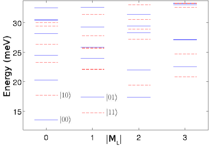
Figure 1: (Color online) Energy levels as functions of the absolute value of the total angular momentum $|M_{L}|$. The full blue (dark gray) lines correspond to singlets and the dashed red (light gray) lines to triplets. The states used to realize the CNOT gate are labeled using the notation $|SM_{L}\rangle$.

Some progress towards quantitative operational quantum gates has been made through suggestions for controlled persistent ring current schemes Tatara and Garcia (2003), and numerical demonstrations of fast coherent control in a one-electron quantum ring Räsänen et al. (2007); DiasdaSilva et al. (2007). In the present letter we have instead analyzed a strongly correlated two-electron quantum ring. For the design of quantum gates in the time domain, a characterization including both electron-electron interactions and realistic system parameters is a prerequisite, and the understanding of the spectrum of excited states is of utmost importance. With such knowledge, it is possible to design an electromagnetic pulse to optimize transitions, as recently shown in the case of a two-electron quantum dot molecule Sælen et al. (2008). For this purpose, we perform an exact diagonalization of the two-electron quantum ring Hamiltonian with realistic model parameters. From the results, we characterize the wave functions in terms of conserved quantum numbers, probability densities and probability currents. Based on this analysis, we propose a new form for quantum information storage and show that a controlled two-bit operation can be performed with almost 100% fidelity.

II Theory

II.1 One electron

The Hamiltonian of one electron confined in a 2D quantum ring, modeled by a displaced harmonic confinement rotated around the $z$-axis, can be written

$$\hat{h}_{s}=\frac{\hat{\mathrm{\textbf{p}}}^{2}}{2m^{*}}+\frac{1}{2}m^{*}\omega_{0}^{2}(r-r_{0})^{2},$$ (1)

where $m^{*}=0.067m_{e}$ is the effective mass of GaAs, $\omega_{0}$ corresponds to the potential strength, $r$ is the radial coordinate and $r_{0}$ the ring radius.

In polar coordinates, the radial equation then reads

$$\left[\frac{\hbar^{2}}{2m^{*}}\left(-\frac{\partial^{2}}{\partial r^{2}}+\frac{m_{l}^{2}}{r^{2}}\right)+\frac{1}{2}m^{*}\omega_{0}^{2}(r-r_{0})^{2}-E\right]u_{nm_{l}}(r)=0,$$ (2)

where $m_{l}$ is the angular quantum number and $u_{nm_{l}}(r)$ is the radial function.

Throughout this work $r_{0}=2$ a.u.${}^{*}\approx 19.6$ nm and $\hbar\omega=10$meV have been used. These potential parameters correspond well to what has been measured in experiments Lorke et al. (2000). Note that we here use the abbreviation a.u.^∗ for effective atomic units, i.e. atomic units that have been rescaled with the material parameters $m^{*}$ and $\epsilon_{r}$.

The one–particle wave functions are then found by the single particle treatment described in section II A of Ref. Waltersson and Lindroth (2007). Here, however, we use a knot sequence that is centered around $r_{0}$ and where the knot points are distributed using an $\arcsin$ function.

II.2 Two electrons

The two–electron Hamiltonian is written as

$$\hat{H}_{0}=\hat{h}_{s}^{1}+\hat{h}_{s}^{2}+\frac{e^{2}}{4\pi\epsilon_{r}\epsilon_{0}\hat{r}_{12}},$$ (3)

where $\epsilon_{r}=12.4$ (GaAs). The corresponding eigenvalues are found by exact diagonalization in a basis set consisting of eigenstates to $\hat{h}_{s}^{1}+\hat{h}_{s}^{2}$, as explained in Ref. Waltersson and Lindroth (2007). The basis set is truncated at $n=13$ and $|m_{l}|=12$, yielding matrix sizes in the order of $5000\times 5000$.

To visualize the many body states we calculate the probability density $\rho$ and probability current j and integrate out the coordinates of one of the electrons,

$$\rho(\mathrm{\textbf{r}}_{1}) = \int d\mathrm{\textbf{r}}_{2}|\Psi(\mathrm{\textbf{r}}_{1},\mathrm{\textbf{r}}_{2})|^{2}$$ (4)

$$\mathrm{\textbf{j}}(\mathrm{\textbf{r}}_{1}) = \Re\left[\int d\mathrm{\textbf{r}}_{2}\Psi^{*}(\mathrm{\textbf{r}}_{1},\mathrm{\textbf{r}}_{2})\left(-\frac{i\hbar}{m^{*}}\nabla_{1}\Psi(\mathrm{\textbf{r}}_{1},\mathrm{\textbf{r}}_{2})\right)\right].$$ (5)

Similarly we calculate the relative probability density $\tilde{\rho}$ and the relative probability current $\tilde{j}$ by the coordinate transformation $\phi_{1}\rightarrow\phi_{rel}=\phi_{1}-\phi_{2}$

$$\tilde{\rho}(r_{1},\phi_{rel}) \equiv \rho(r_{1},\phi_{1}-\phi_{2})$$ (6)

$$\tilde{\mathrm{\textbf{j}}}(r_{1},\phi_{rel}) \equiv \mathrm{\textbf{j}}(r_{1},\phi_{1}-\phi_{2}).$$ (7)

Since there is no preferred angle $\phi$ this is equivalent to freezing one electron at $\phi=0$ and calculating the probability density (current) of the other one.

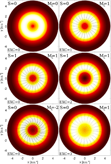
Figure 2: (Color online) Probability densities and currents of the two electron ring plotted in the coordinates of the first electron, see eqs. (4) and (5). The left column depicts the lowest energy states (EXC$=0$) for $M_{L}=0,1$ and $-2$ counting downwards. The right column depicts the first, second and third excited state (EXC$=1,2$ and $3$) with $M_{L}=1$, also counting downwards. Here the ring radius is set to $r_{0}=2$ a.u.${}^{*}\approx 19.6$ nm.

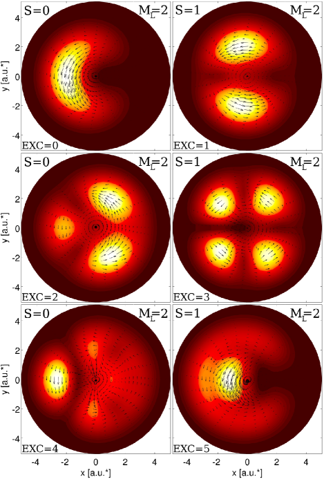
Figure 3: (Color online) Relative probability densities and currents, see eqs. (6) and (7), of the $M_{L}=2$ system. The left column depicts singlets and the right triplets, starting with the lowest lying singlet (triplet) at the top left (right) corner, continuing with the first excited singlet (triplet) in the middle left (right) panel and so on, compare Fig1. The label EXC$=0$ is used for ground states, EXC$=1$ for the first excited state etc. Here the ring radius is set to $r_{0}=2$ a.u.${}^{*}\approx 19.6$ nm.

III Structure of the strongly correlated quantum ring

Fig. 1 shows the energy level scheme. The full blue (dark gray) lines represent spin singlets ($S=0$) and the dashed red (light gray) lines spin triplets ($S=1$). We observe large singlet–triplet splittings, e.g. between the first and second excited $M_{L}=0$ states, caused by the electron-electron interaction representing $\sim 30\%$ of the energy.

Fig. 2 depicts the probability densities and probability currents, eqs. (4) and (5), for a set of different states. The lowest energy state for each $M_{L}$–symmetry are all ring formed and the expected properties; increasing probability currents with increasing $|M_{L}|$ and sign dependent direction of the probability current, are clearly shown. Moreover, both the first and second excited $M_{L}=1$ states are ring formed while the third excited state shows a more dot-like behavior with a relatively large probability density at the center of the system.

In Fig. 3 the relative probability densities and relative probability currents, eq. (6) and (7), of the six lowest lying $M_{L}=2$ states are shown. The lowest lying state has one relative current density peak, the first excited state has two peaks etc, up to the third excited state. These vibrational excitations are expected in a quantum ring Viefers et al. (2003). The fourth and fifth excited state, however, do not continue this quantum ring pattern, indicating that these more energetic states are more dot-like. For the relative probability current, however, signs of deviation from ring behavior are seen earlier. While for a large (or quasi 1D) ring, the radial component of the relative probability currents would approach (be) zero, the currents here show a rich structure. Already at the first excited state, and even more clearly in the higher lying states, we see complete departure from this circular shape. Even probability current vortices can be seen, i.e. between the peaks in the third excited state. Hence, we are here in a region of strongly correlated electrons that still exhibit ring-like behavior.

IV The Controlled NOT operation

The conservation of the total spin ($S$) and angular momentum ($M_{L}$) suggests the possibility to apply these two variables for storage of quantum information, such that one qubit is represented by $S$ and another multivalued “quMbit” is stored in $M_{L}$. Single qubit operations involving the latter may then be performed by carefully optimized spin conserving electromagnetic interactions Sælen et al. (2008). Controlled spin manipulation will in general be more complicated but can be performed by various schemes involving inhomogeneous magnetic fields Fuhrer et al. (2001, 2003). The control of the time-scale of the two single-qubit operations will be a matter of magnetic field inhomogeneity vs. size of the quantum ring: Experimentally, the degree of inhomogeneity is allowed to increase with the ring-size, thereby decreasing the spin flip period. The transition period between electronic states, that for small radii are much shorter, will on the other hand increase with the ring radius. At some point, both of these single qubit operations can be performed at comparable time scales.

The critical and remaining question is thus whether two-qubit operations can be performed in such a way that a change of an initial $|S,M_{L}\rangle$ can take place for a conditional value of $S$. The relatively strong electron-electron interaction can here play a constructive role as it changes the electronic energy shift between internal singlet and triplet states, cf. Fig. 1. In this way, the ring size can be used as a parameter to tune the energy spectrum. Fig. 4 depicts the quotient between $E_{|10\rangle}-E_{|11\rangle}$ and $E_{|01\rangle}-E_{|00\rangle}$ (see Fig.1) as a function of the ring radius $r_{0}$. Starting at unity for $r_{0}=0$, this quotient decreases to a minimum at $r_{0}\approx 3$ a.u.* and then increases again for larger ring radii. To realize a conditional operation we want this quotient to be as far from unity as possible. However, to protect the CNOT against decoherence we want the absolute value of both energy differences to be large. These energy differences decrease monotonically with the ring radius, see insert of Fig. 4, yielding better protection for smaller radii. Weighting these two things together, a ring radius $\sim 2$ a.u.* seems a close to optimal choice.

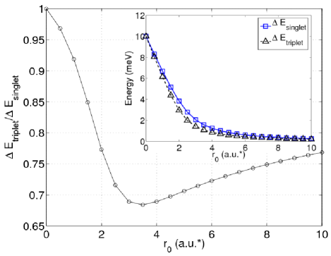
Figure 4: (Color online) The quotient between $\Delta E_{\textrm{triplet}}=E_{|10\rangle}-E_{|11\rangle}$ and $\Delta E_{\textrm{singlet}}=E_{|01\rangle}-E_{|00\rangle}$ (see Fig.1) as a function of the ring radius $r_{0}$. The insert shows the absolute value of $\Delta E_{\textrm{triplet}}$ and $\Delta E_{\textrm{singlet}}$ as a function of the same. Here the effective Bohr radius $=1$ a.u* $\approx 9.8$ nm.

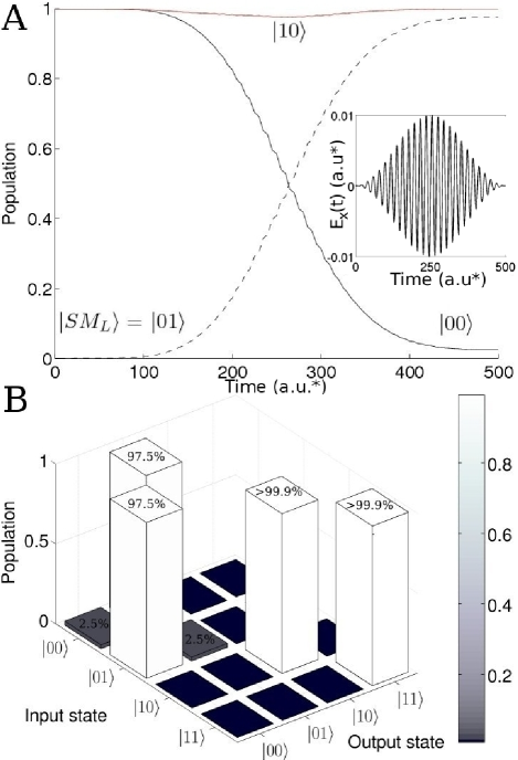
Figure 5: (Color online) Upper panel: The time development of the populations of the different states when the central frequency, $\omega_{L}$, of the pulse corresponds to the energy shift between the the two lowest states in the singlet system, $\Delta\varepsilon_{|SM_{L}\rangle}=\varepsilon_{|01\rangle}-\varepsilon_{|00\rangle}\approx 3.8$ meV implying a laser frequency of $0.9$ Thz. The population of the state $|SM_{L}\rangle=|00\rangle$ is almost completely transferred to $|01\rangle$, while the population of the $|10\rangle$ is seen to be nearly constant. The insert shows the $x$-component of the electromagnetic pulse. Lower panel: The truth table shows just a small amount of unwanted population. The pulse length was chosen to be $T=500$ a.u* $\approx 28$ps.

IV.1 The interaction with the electromagnetic field

We now examine transitions induced by a circularly polarized electromagnetic pulse ${\bf E}(t)=E(t)[\cos{(\omega_{L}t)}\hat{\mathrm{\textbf{x}}}\pm\sin{(\omega_{L}t)}\hat{\mathrm{\textbf{y}}}]$ where $\omega_{L}$ is the central frequency. The electric dipole interaction then couples neighboring $M_{L}$ states ($\Delta M_{L}=1$). The envelope $E(t)$ is taken as, $E(t)=E_{0}\sin^{2}\left(\pi t/T\right)$, which defines a pulse that lasts from $t=0$ to $t=T$. Here we set $T=500$ a.u.${}^{*}\approx 28$ ps and $E_{0}\approx 0.01$ a.u.^∗ corresponding to an intensity $\sim 2.4\cdot 10^{2}$W/cm². We solve the time dependent Schrödinger equation in the full basis of eigenstates obtained from the previous diagonalization. The Hamiltonian then becomes

$$\hat{H}(t)=\hat{H}_{0}+e\mathrm{\textbf{E}}(t)\cdot(\mathrm{\textbf{r}}_{1}+\mathrm{\textbf{r}}_{2}).$$ (8)

It is then readily shown that the time dependent Schrödinger equation can be written as a coefficient equation including the transition matrix elements from (the two particle) state $|j\rangle$ to state $\langle i|$

$$\dot{c}_{i}(t)=-i\sum_{j}c_{j}(t)e\mathrm{\textbf{E}}(t)\cdot\langle i|(\mathrm{\textbf{r}}_{1}+\mathrm{\textbf{r}}_{2})|j\rangle.$$ (9)

IV.2 The realization of the CNOT

Fig. 5A depicts the time development of the populations of the different states when the pulse central frequency, $\omega_{L}$, corresponds to the energy shift between the two lowest states in the singlet system $\Delta\varepsilon_{|SM_{L}\rangle}=\varepsilon_{|01\rangle}-\varepsilon_{|00\rangle}\approx 3.8$ meV. The driving laser frequency would then be $\omega_{L}/2\pi\approx 0.9$ THz. With the initial state being $|SM_{L}\rangle=|00\rangle$, we observe a nearly complete transition to $|01\rangle$, with a small amount of unwanted population. Also shown is the time development of the population of an initial $|10\rangle$ which is seen to be nearly constant. Thus a CNOT is realized, as clarified in the truth table of Fig. 5B. It clearly depicts how the electromagnetic pulse transfer $\sim 97.5\%$ of the spin singlet population while leaving $>99.9\%$ of the triplet population unchanged.

V Decoherence, advantages and possible improvements

The natural life time of the excited state is dominated by phonon relaxation and is at least a few orders of magnitudes longer than the time for the induced transition studied here Bockelmann and Bastard (1990). As shown recently, the pulse induced transition time may then be decreased by a factor 10-100 through quantum optimization field control methods optimized to almost any fidelity Sælen et al. (2008); DiasdaSilva et al. (2007). Transition times will also be drastically reduced by increased confinement strength which will lead to considerably higher central frequencies, $\omega_{L}$. In the present work, however, we wanted to examine a region of confinement strengths that already is accessible in experiments Lorke et al. (2000).

The present proposal has certain advantages compared to single quantum dot qubit systemsKoppens et al. (2006). First, the energy difference between the spin states prohibit unwanted transitions up to the order of 10 Kelvin. In the quantum molecule qubit, the energy differences are typically $10^{3}$ times smallerTaylor et al. (2007). Furthermore, by taking advantage of a long array of accessible $M_{L}$ levels, one may develop much more powerful algorithms for certain operations than systems with only two levels.

VI Summary and conclusions

In conclusion we have shown that quantum controlled operations defining a conditional two-bit transition can be realized in a two-electron quantum ring. This has been achieved through a detailed analysis of energy levels and properties of the wave functions. The electron-electron interaction has been utilized to effectively store quantum information simultaneously in the total spin and total angular momentum. We have shown that with realistic model parameters it is possible to find a regime where the singlet and triplet splittings differ such that an electromagnetic pulse can transfer population of one spin state to a higher energy level, while leaving the population of the other spin state intact. This opens for a new type of solid state quantum information devices, for which quantum rings are shown to be promising candidates.

References

- Cirac and Zoller (1995) J. I. Cirac and P. Zoller, Phys. Rev. Lett. 74, 4091 (1995).
- Sørensen and Mølmer (1999) A. Sørensen and K. Mølmer, Phys. Rev. Lett. 82, 1971 (1999).
- Lukin et al. (2001) M. D. Lukin, M. Fleischhauer, R. Cote, L. M. Duan, D. Jaksch, J. I. Cirac, and P. Zoller, Phys. Rev. Lett. 87, 037901 (2001).
- Loss and DiVincenzo (1998) D. Loss and D. P. DiVincenzo, Phys. Rev. A 57, 120 (1998).
- Amlani et al. (1999) I. Amlani, A. O. Orlov, G. Toth, G. H. Bernstein, C. S. Lent, and G. L. Snider, Science 284, 289 (1999).
- Petta et al. (2004) J. R. Petta, A. C. Johnson, C. M. Marcus, M. P. Hanson, and A. C. Gossard, Phys. Rev. Lett. 93, 186802 (2004).
- Taylor et al. (2007) J. M. Taylor, J. R. Petta, A. C. Johnson, A. Yacoby, C. M. Marcus, and M. D. Lukin, Phys. Rev. B 76, 035315 (2007).
- Meunier et al. (2007) T. Meunier, I. T. Vink, L. H. WillemsvanBeveren, K. J. Tielrooij, R. Hanson, F. H. L. Koppens, H. P. Tranitz, W. Wegscheider, L. P. Kouwenhoven, and L. M. K. Vandersypen, Phys. Rev. Lett. 98, 126601 (2007).
- Sælen et al. (2008) L. Sælen, R. Nepstad, I. Degani, and J. P. Hansen, Phys. Rev. Lett. 100, 046805 (2008).
- Robledo et al. (2008) L. Robledo, J. Elzerman, G. Jundt, M. Atatüre, A. Högele, S. Fält, and A. Imamoglu, Science 320, 772 (2008).
- Li et al. (2003) X. Li, Y. Wu, D. Steel, D. Gammon, T. H. Stievater, D. S. Katzer, D. Park, C. Piermarocchi, and L. J. Sham, Science 301, 809 (2003).
- Oosterkamp et al. (1998) T. H. Oosterkamp, T. Fujisawa, W. G. van der Wiel, K. Ishibashi, R. V. Hijman, S. Tarucha, and L. P. Kouwenhoven, Nature 395, 873 (1998).
- van der Wiel et al. (2006) W. G. van der Wiel, M. Stopa, T. Kodera, T. Hatano, and S. Tarucha, New Journal of Physics 8, 28 (2006), URL http://stacks.iop.org/1367-2630/8/28.
- Koppens et al. (2006) F. H. L. Koppens, C. Buizert, K. J. Tielrooij, I. T. Vink, K. C. Nowack, T. Meunier, L. P. Kouwenhoven, and L. M. K. Vandersypen, Nature 442, 766 (2006).
- Warburton et al. (2000) R. J. Warburton, D. H. C. Schäflein, F. Bickel, A. Lorke, K. Karrai, J. M. Garcia, W. Schoenfeld, and P. M. Petroff, Nature 405, 926 (2000).
- Simonin et al. (2004) J. Simonin, C. R. Proetto, Z. Barticevic, and G. Fuster, Phys. Rev. B 70, 205305 (2004).
- Alen et al. (2005) B. Alen, J. Martinez-Pastor, D. Granados, and J. M. Garcia, Phys. Rev. B 72, 155331 (2005).
- Climente et al. (2006) J. I. Climente, J. Planelles, M. Barranco, F. Malet, and M. Pi, Phys. Rev. B 73, 235327 (2006).
- Fuhrer et al. (2001) A. Fuhrer, S. Lüscher, T. Ihn, T. Heinzel, K. Ensslin, W. Wegscheider, and M. Bichler, Nature 413, 822 (2001).
- Fuhrer et al. (2003) A. Fuhrer, T. Ihn, K. Ensslin, W. Wegscheider, and M. Bichler, Phys. Rev. Lett. 91, 206802 (2003).
- Viefers et al. (2003) S. Viefers, P. Koskinen, P. S. Deo, and M. Manninen, Physica E 21, 1 (2003).
- Planelles et al. (2001) J. Planelles, W. Jaskólski, and J. I. Aliaga, Phys. Rev. B 65, 033306 (2001).
- Gudmundsson et al. (2003) V. Gudmundsson, C.-S. Tang, and A. Manolescu, Phys. Rev. B 67, 161301(R) (2003).
- Chakraborty and Pietiläinen (1994) T. Chakraborty and P. Pietiläinen, Phys. Rev. B 50, 8460 (1994).
- Saiga et al. (2007) Y. Saiga, D. S. Hirashima, and J. Usukura, Phys. Rev. B 75, 045343 (2007).
- Hu et al. (2000) H. Hu, J.-L. Zhu, and J.-J. Xiong, Phys. Rev. B 62, 16777 (2000).
- Fomin et al. (2008) V. M. Fomin, V. N. Gladilin, J. T. Devreese, N. A. J. M. Kleemans, and P. M. Koenraad, Phys. Rev. B 77, 205326 (2008).
- Puente and Serra (2001) A. Puente and L. Serra, Phys. Rev. B 63, 125334 (2001).
- Tatara and Garcia (2003) G. Tatara and N. Garcia, Phys. Rev. Lett. 91, 076806 (2003).
- Räsänen et al. (2007) E. Räsänen, A. Castro, J. Werschnik, A. Rubio, and E. K. U. Gross, Phys. Rev. Lett. 98, 157404 (2007).
- DiasdaSilva et al. (2007) L. G. G. V. DiasdaSilva, J. M. Villas-Boas, and S. E. Ulloa, Phys. Rev. B 76, 155306 (2007).
- Lorke et al. (2000) A. Lorke, R. J. Luyken, A. O. Govorov, J. P. Kotthaus, J. M. Garcia, and P. M. Petroff, Phys. Rev. Lett. 84, 2223 (2000).
- Waltersson and Lindroth (2007) E. Waltersson and E. Lindroth, Phys. Rev. B 76, 045314 (2007).
- Bockelmann and Bastard (1990) U. Bockelmann and G. Bastard, Phys. Rev. B 42, 8947 (1990).