Many-Body perturbation theory calculations on circular quantum dots

Abstract

The possibility to use perturbation theory to systematically improve calculations on circular quantum dots is investigated. A few different starting points, including Hartree-Fock, are tested and the importance of correlation is discussed. Quantum dots with up to twelve electrons are treated and the effects of an external magnetic field are examined. The sums over excited states are carried out with a complete finite radial basis set obtained through the use of B-splines. The calculated addition energy spectra are compared with experiments and the implications for the filling sequence of the third shell are discussed in detail.

I Introduction

During the last decade a new field on the border between condensed matter physics and atomic physics has emerged. Modern semi-conductor techniques allow fabrication of electron quantum confinement devices, called quantum dots, containing only a small and controllable number of electrons. The experimental techniques are so refined that one electron at a time can be injected into the dot in a fully controllable way. This procedure has shown many similarities between quantum dots and atoms, for example the existence of shell structure. To emphasize these similarities quantum dots are often called artificial atoms. The interest in quantum dots is mainly motivated by the fact that their properties are tunable through electrostatic gates and external electric and magnetic fields, making these designer atoms promising candidates for nanotechnological applications. An additional aspect is that quantum dots provide a new type of targets for many-body methods. In contrast to atoms they are essentially two-dimensional and their physical size is several orders of magnitude larger than that of atoms, leading e.g. to a much greater sensitivity to magnetic fields. Another difference compared to atoms is the strength of the overall confinement potential relative to that of the electron-electron interaction, which here varies over a much wider range.

The full many-body problem of quantum dots is truly complex. A dot is formed when a two-dimensional electron gas in an heterostructure layer interface is confined also in the $xy$–plane. The, for this purpose applied gate voltage, results in a potential well, the form of which is not known. A quantitative account of this trapping potential is one of the quantum dot many-body problems. Self-consistent solutions of the combined Hartree and Poisson equations by Kumar et al. Kumar et al. (1990) in the early nineties indicated that for small particle numbers this confining potential is parabolic in shape at least to a first approximation. Since then a two-dimensional harmonic oscillator potential have been the standard choice for studies concentrating on the second many-body problem of quantum dots; that of the description of the interaction among the confined electrons. The efforts to give a realistic description of the full physical situation, see e.g. Kumar et al. (1990); Jovanovic and Leburton (1994); Matagne et al. (2002); Matagne and Leburton (2002); Melnikov et al. (2005) have, however, underlined that it is important to realize the limits of this choice. To start with the pure parabolic potential seems to be considerably less adequate when the number of electrons is approaching twenty. The potential strength is further not independent of the number of electrons put into the dot, an effect which is sometimes approximately accounted for by decreasing the strength with the inverse square root of the number of electrons Koskinen et al. (1997). Finally, the assumption that the confining potential is truly two-dimensional is certainly an approximation and it will to some extent exaggerate the Coulomb repulsion between the electrons. In Ref. Matagne et al. (2002) the deviation from the pure two-dimensional situation is shown to effectively take the form of an extra potential term scaling with the fourth power of the distance to the center and which can be both positive and negative. Although the deviation is quite small it is found that predictions concerning the so called third shell can be affected by it.

There is thus a number of uncertainties in the description of quantum dots. On the one hand there is the degree to which real dots deviate from two-dimensionality and pure parabolic confinement. On the other hand there is the uncertainty in the account of electron correlation among the confined electrons. The possible interplay among these uncertainties is also an open question. In a situation like this it is often an advantage to study one problem at a time, since it is then possible to have control over the approximations made and quantify their effects. We concentrate here on the problem of dot-electron correlation. For this we employ a model dot; truly two-dimensional, with perfect circular symmetry and with a well defined strength of the confining potential. This choice is sufficient when the aim is to test the effects of the approximations introduced through the approximative treatment of the electron-electron interaction.

Especially the experimental study by Tarucha et. al. Tarucha et al. (1996) has worked as a catalyst for a vast number of theoretical studies of quantum dots. A review of the theoretical efforts until a few years ago has been given by Reimann and Manninen Reimann and Manninen (2002). A large number of calculations has been done within the framework of Density Functional Theory (DFT) Koskinen et al. (1997); Macucci et al. (1997); Lee et al. (1998); Reimann and Manninen (2002) and reference therein, but also Hartree–Fock (HF) Fujito et al. (1996); Bednarek et al. (1999); Yannouleas and Landman (1999), Quantum Monte Carlo methods Ghosal and Güçlü (2006); Saarikoski and Harju (2005) and Configuration Interaction (CI) Reimann et al. (2000); Bruce and Maksym (2000); Szafran et al. (2003) studies have been performed. The DFT–studies have been very successful. The method obviously accounts for a substantial part of the electron-electron interaction. Still, the situation is not completely satisfactory since there is no possibility to systematically improve the calculations or to estimate the size of neglected effects. For just a few electrons the CI-approach can produce virtually exact results, provided of course that the basis set describes the physical space well enough. The size of the full CI problem grows, however, very fast with the number of electrons and to the best of our knowledge the largest number of electrons in a quantum dot studied with CI is six. It would be an advantage to also have access to a many-body method which introduces only well defined approximations and which allows a quantitative estimate of neglected contributions. The long tradition of accurate calculations in atomic physics has shown that Many-Body Perturbation Theory (MBPT) has these properties. It is an in principle exact method, applicable to any number of electrons, and the introduced approximations are precisely defined. With MBPT it is possible to start from a good, or even reasonable, description of the artificial atom and then refine this starting point in a controlled way. We are only aware of one study on quantum dots that have been done with MBPT, the one by Sloggett and SushkovSloggett and Sushkov (2005). They did second–order correlation calculations on circular and elliptical dots in an environment free of external fields.

In the present study we use second–order perturbation theory to calculate energy spectra for quantum dots with and without external magnetic fields. We consider this second–order treatment as a first step towards the calculation of correlation to high orders through iterative procedures, an approach commonly used for atoms Lindgren and Morrison (1986). The method is described in Section II. In section  III we compare our calculations with experimental resultsTarucha et al. (1996); Matagne et al. (2002), DFT–calculations Reimann et al. (2000) and CI–calculations, our own as well as those of Reimann et al. Reimann et al. (2000) and discuss the strength and limits of the MBPT approach. We have mainly used the Hartree-Fock description as starting point for the perturbation expansion, but we also show examples with a few alternative starting points, among them DFT. To obtain a complete and finite basis set, well suited to carry out the perturbation expansion, we use so called B-splines, see e.g. Ref. deBoor (1978). The use of B-splines in atomic physics was pioneered by Johnson and Sapirstein Johnson and Sapirstein (1986) twenty years ago and later it has been the method of choice in a large number of studies as reviewed e.g. in Ref. Bachau et al. (2001). We compare our correlated results to our own HF–calculations, thereby highlighting the importance of correlation both when the quantum dot is influenced by an external magnetic field and when it is not. We present addition energy spectra for the first twelve electrons. The interesting third shell (electron seven to twelve) is discussed in Section IV. Here we investigate several different filling sequences and show that correlation effects in many cases can change the order of which the shells are filled. We note also that the energy of the first excited state can be very close to the ground state, in some case less than 0.1 meV, which raises the question if it is always the ground state which is filled when an additional electron is injected in the dot since more than one state may lie in the transport window controlled by the source drain voltage Kouwenhoven et al. (1997).

II Method

The essential point in perturbation theory is to divide the full Hamiltonian $\hat{H}$ into a first approximation, $\hat{h}$, and a correction, $\hat{U}$. The first approximation should be easily obtainable, in practice it is more or less always chosen to be an effective one-particle Hamiltonian, and it should describe the system well enough to ensure fast and steady convergence of the perturbation expansion. The partition is written as

$$\hat{H}=\sum_{i=1}^{N}\hat{h}(i)+\hat{U}.$$ (1)

Here we have chosen to mainly use the Hartree-Fock Hamiltonian as $\hat{h}$ but we have also investigated the possibility to use a few other starting points.

A first approximation to the energy is obtained from the expectation value of $\hat{H}$, calculated with a wave function in the form of a Slater determinant formed from eigenstates to $\hat{h}(i)$. The result is then subsequently refined through the perturbation expansion. Below we describe the calculations step by step.

II.1 Single-particle treatment

For a single particle confined in a circular quantum dot the Hamiltonian reads

$$\hat{h}_{s}=\frac{\mathbf{\hat{p}}^{2}}{2m^{*}}+\frac{1}{2}m^{*}\omega^{2}r^{2}+\frac{e^{2}}{8m^{*}}B^{2}r^{2}+\frac{e}{2m^{*}}B\hat{L}_{z}+g^{*}\mu_{b}B\hat{S}_{z},$$ (2)

where B is an external magnetic field applied perpendicular to the dot. The effective electron mass is denoted with $m^{*}$ and the effective g-factor with $g^{*}$. Throughout this work we use $m^{*}=0.067m_{e}$ and $g^{*}=-0.44$, corresponding to bulk values in GaAs.

The single particle wave functions separate in polar coordinates as

$$|\Psi_{nm_{\ell}m_{s}}\rangle=|u_{nm_{\ell}m_{s}}(r)\rangle|e^{im_{\ell}\phi}\rangle|m_{s}\rangle.$$ (3)

As discussed in the introduction we expand the radial part of our wave functions in so called B-splines labeled $B_{i}$ with coefficients $c_{i}$, i.e.

$$|u_{nm_{\ell}m_{s}}(r)\rangle=\sum_{i=1}c_{i}|B_{i}(r)\rangle.$$ (4)

B–splines are piecewise polynomials of a chosen order $k$, defined on a so called knot sequence and they form a complete set in the space defined by the knot sequence and the polynomial order deBoor (1978). Here we have typically used $40$ points in the knot sequence, distributed linearly in the inner region and then exponentially further out. The last knot, defining the box to which we limit our problem is around 400 nm. The polynomial order is six and combined with the knot sequence this yield $33$ radial basis functions, $u_{nm_{\ell}m_{s}}(r)$, for each combination $(m_{\ell},m_{s})$. The lower energy basis functions are physical states, while the higher ones are determined mainly by the box. The unphysical higher energy states are, however, still essential for the completeness of the basis set.

Eqs. (3) and (4) imply that the Schrödinger equation can be written as a matrix equation

$$\mathbf{Hc}=\epsilon\mathbf{Bc}$$ (5)

where $H_{ji}=\langle B_{j}e^{im\theta}|\hat{H}|B_{i}e^{im\theta}\rangle$ and $B_{ji}=\langle B_{j}|B_{i}\rangle$ .

Eq.( 5) is a generalized eigenvalue problem that can be solved with standard numerical routines. The integrals in (5) are calculated with Gaussian quadrature and since B-splines are piecewise polynomials this implies that essentially no numerical error is produced in the integration.

II.2 Many-Body treatment

The next step is to allow for several electrons in the dot and then to account for the electron-electron interaction,

$$\frac{e^{2}}{4\pi\epsilon_{r}\epsilon_{0}}\frac{1}{\mid\mathbf{r}_{i}-\mathbf{r}_{j}\mid},$$ (6)

where $\epsilon_{r}$ is the relative dielectric constant which in the following calculations is taken to be $\epsilon_{r}=12.4$ corresponding to the bulk value in GaAs. For future convenience we define the electron–electron interaction matrix element as

$$\langle ab|\frac{1}{\hat{r}_{ij}}|cd\rangle=\int\!\!\!\int\frac{e^{2}\Psi_{a}^{*}(\mathbf{r}_{i})\Psi_{b}^{*}(\mathbf{r}_{j})\Psi_{c}(\mathbf{r}_{i})\Psi_{d}(\mathbf{r}_{j})}{4\pi\epsilon_{r}\epsilon_{0}|\mathbf{r}_{i}-\mathbf{r}_{j}|}dA_{i}dA_{j},$$ (7)

where $a,b,c$ and $d$ each denote a single quantum state i.e. $|a\rangle=|n^{a},m^{a}_{\ell},m^{a}_{s}\rangle$.

II.2.1 The Multipole expansion

As suggested by Cohl et. alCohl et al. (2001), the inverse radial distance can be expanded in cylindrical coordinates $(R,\phi,z)$ as

$$\frac{1}{|\mathbf{r}_{1}-\mathbf{r}_{2}|}=\frac{1}{\pi\sqrt{R_{1}R_{2}}}\sum_{m=-\infty}^{\infty}Q_{m-\frac{1}{2}}(\chi)e^{im(\phi_{1}-\phi_{2})},$$ (8)

where

$$\chi=\frac{R_{1}^{2}+R_{2}^{2}+(z_{1}-z_{2})^{2}}{2R_{1}R_{2}}.$$ (9)

Assuming a 2D confinement we set $z_{1}=z_{2}$ in (9). The $Q_{m-\frac{1}{2}}(\chi)$–functions are Legendre functions of the second kind and half–integer degree. We evaluate them using a modified version of software DTORH1.f described inSegura and Gil (1999).

Using (8) and (3) the electron–electron interaction matrix element (7) becomes

$$\langle ab|\frac{1}{\hat{r}_{12}}|cd\rangle=\frac{e^{2}}{4\pi\epsilon_{r}\epsilon_{0}}\langle u_{a}(r_{i})u_{b}(r_{j})|\frac{Q_{m-\frac{1}{2}}(\chi)}{\pi\sqrt{r_{i}r_{j}}}|u_{c}(r_{i})u_{d}(r_{j})\rangle$$

$$\times\langle e^{im_{a}\phi_{i}}e^{im_{b}\phi_{j}}|\sum_{m=-\infty}^{\infty}e^{im(\phi_{i}-\phi_{j})}|e^{im_{c}\phi_{i}}e^{im_{d}\phi_{j}}\rangle$$

$$\times\langle m_{s}^{a}|m_{s}^{c}\rangle\langle m_{s}^{b}|m_{s}^{d}\rangle.$$ (10)

Note that the angular part of (II.2.1) equals zero except if $m=m_{a}-m_{c}$ or $m=m_{d}-m_{b}$. This is how the degree of the Legendre–function in the radial part of (II.2.1) is chosen. It is also clear from (II.2.1) that the electron–electron matrix element (7) equals zero if state $a$ and $c$ or state $b$ and $d$ have different spin directions.

II.2.2 Hartree–Fock

If the wave function is restricted to be in the form of a single Slater determinant, the Hartree-Fock approximation can be shown to yield the lowest energy. In this approximation each electron is governed by the confining potential and an average Hartree-Fock potential formed by the other electrons. To account for the latter the Hamiltonian matrix $\mathbf{H}$ in Eq. (5) is modified by the addition of a term:

$$u^{HF}_{ji}=\langle B_{j}|\hat{u}_{HF}|B_{i}\rangle=\sum_{a\leq N}\langle B_{j}a|\frac{1}{\hat{r}_{12}}|B_{i}a\rangle-\langle B_{j}a|\frac{1}{\hat{r}_{12}}|aB_{i}\rangle.$$ (11)

The sum here runs over all occupied orbitals, $a$, defined by quantum numbers $n$, $m_{\ell}$, and $m_{s}$. Eq. (5) is then solved iteratively yielding new and better wave functions in each iteration until the energies become self–consistent. The hereby obtained solution is often labeled the unrestricted Hartree-Fock approximation since no extra constraints are imposed on $u^{HF}$.

One property of the unrestricted Hartree–Fock approximation deserves special attention. Consider the effects of the Hartree-Fock potential on an electron in orbital $b$,

$$\langle b|\hat{u}_{HF}|b\rangle=\sum_{a\leq N}\langle ba|\frac{1}{\hat{r}_{12}}|ba\rangle-\langle ba|\frac{1}{\hat{r}_{12}}|ab\rangle,$$ (12)

where the last term in Eq. (12), the exchange term, is non-zero only if orbital $a$ and $b$ have the same spin. For configurations where not all electron spins are paired electrons with the same quantum numbers $n$ and $m_{\ell}$, but with different spin directions, will experience different potentials. This is in accordance with the physical situation, but has also an undesired consequence; the total spin, ${\bf S}^{2}=\left(\sum_{i}{\bf s}_{i}\right)^{2}$, does not commute with the Hartree-Fock Hamiltonian. This means that the state vector constructed as a single Slater determinant of Hartree–Fock orbitals will not generally be a spin eigenstate. However, the full Hamiltonian, Eq. 1, still commutes with ${\bf S}^{2}$ and during the perturbation expansion the spin will eventually be restored, provided of course that the perturbation expansion converges. Since, in contrast to the energy, the total spin of a state is usually known, the expectation value of the total spin, $\langle{\bf S}^{2}\rangle$, can be used as a measure of how converged the perturbation expansion is. It can also be used as an indication of when the Hartree–Fock description is too far away from the physical situation to be a good enough starting point. This is discussed further in Sections III and IV.

II.2.3 second–order correction to a Hartree–Fock starting point

The leading energy correction to the Hartree–Fock starting point is of second order in the perturbation (defined in Eq. (1)). When $\hat{h}=\hat{h}_{s}+\hat{u}_{HF}$ and $\hat{U}=\sum_{i<j}\frac{1}{\hat{r}_{ij}}-\sum_{i=1}^{N}\hat{u}_{HF}(i)$, the corresponding corrections to the wave function will not include any single excitations. This is usually referred to as Brillouin’s theorem and is discussed in standard Many–Body theory textbooks, see e.g. Lindgren and MorrisonLindgren and Morrison (1986). Starting from the HF–Hamiltonian for $N$ electrons in the dot we write the second–order correction to the energy

$$\delta E_{N}^{(2)}=\sum_{a<b\leq N}\sum_{\begin{subarray}{c}r,s>N\\ r\neq s\end{subarray}}\frac{|\langle rs|\frac{1}{\hat{r}_{12}}|ab\rangle|^{2}-\langle ba|\frac{1}{\hat{r}_{12}}|rs\rangle\langle rs|\frac{1}{\hat{r}_{12}}|ab\rangle}{\epsilon_{a}+\epsilon_{b}-\epsilon_{r}-\epsilon_{s}}$$ (13)

where thus both $r$ and $s$ are unoccupied states.

Since B–splines are used for the expansion of the radial part of the wave functions there is a finite number of radial quantum numbers ($n$) to sum over in the second sum of Eq. (13). However, in principle there is still an infinite number of angular quantum numbers ($m_{\ell}$) to sum over in the same sum. In praxis this summation has to be truncated and the effects of this truncation will be discussed in section III.

II.2.4 Other starting points than Hartree-Fock

In principle any starting point, with wave functions close enough to the true wave functions (to ensure convergence of the perturbation expansion), can work as a starting point for MBPT. We have in addition to HF investigated three alternative starting points. If there are important cancellations between the full exchange (included in Hartree-Fock) and correlation (not included in Hartree-Fock) an alternative starting point might converge faster, or even provide convergence in regions where it cannot be achieved with Hartree-Fock. First of all we start with the simplest possible starting point; the pure one–electron wave functions. In this case the basis set consists of the solutions to the pure 2D harmonic oscillator in the chosen box and we treat the whole electron–electron interaction as the perturbation. The second alternative starting point is the Local Density Approximation (LDA). That is we switch the second term in Eq. (11) to $\alpha\langle B_{j}|4a_{B}^{*}\sqrt{\frac{2\rho(r)}{\pi}}|B_{i}\rangle$, where $\rho(r)$ is the radial electron density and $\alpha$ is called Slaters exchange parameter and is usually set to one. Both these starting Hamiltonians are defined with only local potentials and will thus commute with the total spin. The third alternative starting point is a reduced exchange HF, i.e. the exchange term (the second term) in Eq. (11) is simply multiplied with a constant $\alpha<1$. When using these alternative starting points, one must in contrast to the Hartree-Fock case include single excitations in the perturbation expansion.

The second–order perturbation correction then becomes

$$\delta E_{N}^{(2)}=\sum_{a,b<N}\sum_{r>N}\frac{|\langle r|\hat{V}_{ex}|a\rangle-\langle rb|\frac{1}{r_{12}}|ba\rangle|^{2}}{\epsilon_{a}-\epsilon_{r}}+$$

$$\sum_{a<b\leq N}\sum_{\begin{subarray}{c}r,s>N\\ r\neq s\end{subarray}}\frac{|\langle rs|\frac{1}{\hat{r}_{12}}|ab\rangle|^{2}-\langle ba|\frac{1}{\hat{r}_{12}}|rs\rangle\langle rs|\frac{1}{\hat{r}_{12}}|ab\rangle}{\epsilon_{a}+\epsilon_{b}-\epsilon_{r}-\epsilon_{s}}$$ (14)

where $\hat{V}_{ex}$ is the chosen exchange operator. From this expression it is also clear that the first term yields zero in the pure Hartree–Fock case, i.e. then all single excitations cancel.

II.2.5 Full CI treatment of the two body problem

To investigate how well second–order many-body perturbation theory performs we have for the simple case of two electrons also solved the full CI problem. We then diagonalize the matrix that consists of all the elements of the form

$$H_{ji}=\left\langle mn\right|_{j}\>\hat{h}_{s}^{1}+\hat{h}_{s}^{2}+\frac{1}{\hat{r}_{12}}\>|op\rangle_{i}$$ (15)

for given values of $M_{L}=\sum m_{\ell}$ and $M_{S}=\sum m_{s}$ of our electron pairs $\{|mn\rangle_{i}\}$. Following the selection rules produced by Eq. (II.2.1) we get the conditions $m_{\ell}^{o}+m_{\ell}^{p}=m_{\ell}^{m}+m_{\ell}^{n}$, $m_{s}^{m}=m_{s}^{o}$ and $m_{s}^{n}=m_{s}^{p}$.

III Validation of the Method

The main purpose of this work is to investigate the usability of many body perturbation theory on (GaAs) quantum dots. Therfore we have in this section compared our results with results from other theoretical works.

Our energies are generally given in meV. For easy comparison with other calculations it should be noted that the scaled atomic unit for energy is $1\,\,\mathrm{Hartree}^{*}=1\,\,\mathrm{Hartree}\,\left(m^{*}/(m_{e}\varepsilon_{r}^{2})\right)\approx 11.857$ meV, with $m^{*}=0.067m_{e}$ and $\varepsilon_{r}=12.4$. The scaled Bohr radius is $a_{B}^{*}=\left(\varepsilon_{r}m_{e}/m^{*}\right)a_{B}\approx 9.794$ nm.

III.1 The two electron dot

Fig. 1 shows the second–order many–body perturbation correction to the energy, Eq. (13), as function of max$(n)$ (squares) and max$(|m_{\ell}|)$ (circles) respectively for the two electron dot with $\hbar\omega=6$ meV. It clearly illustrates that both curves converge but also that the sum over $m_{\ell}$ converges faster than the sum over $n$. Due to this we have throughout our calculations used all radial basis functions and as many angular basis functions that are needed for convergence. One should, however, notice that the relative convergence as a function of max$(n)$ and max$(|m_{\ell}|)$ varies with the confinement strength and occupation number. Weak potentials ($\hbar\omega<2$ meV) usually produce the opposite picture i.e. a faster convergence for $n$ than for $m_{\ell}$. For confinement strengths ($\hbar\omega>3$ meV) and most occupation numbers the trend shown in Fig. (1) is, however, typical.

Figure 1: Second–order perturbation theory correction to the energy as function of max$(n)$ (squares) and max$(|m_{\ell}|)$ (circles) in the second sum of Eq. (13) for the two electron dot with the confinement strength $\hbar\omega=6$ meV. Note that the sum over $m_{\ell}$ converges faster than the sum over $n$.

III.1.1 Comparison between different starting points

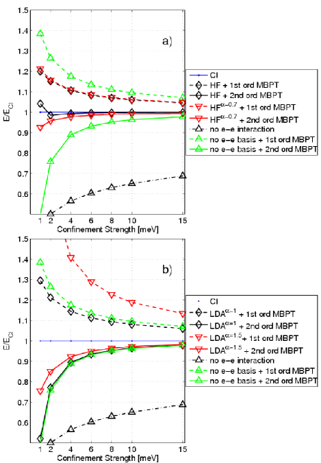
Figure 2: The quotient between the calculated energies (of respective method) and the CI–energy as functions of the confinement strength, $\hbar\omega$, for the ground state in the two electron dot. In a) the results from HF, a reduced exchange HF with $\alpha=0.7$ and 2nd order MBPT using wave functions from respective method are plotted. In b) the results from LDA-calculations (with two different alphas) + 1st and 2nd order MBPT are plotted. For reference the results from calculations where we have used the one-electron wave functions as a starting point for the perturbation expansion (taking the whole electron-electron interaction as the perturbation) have been plotted in both a) and b).

In Fig. 2 a) and b) comparisons between HF (i.e. the expectation value of the full Hamiltonian with a Slater determinant of Hartree-Fock orbitals, labelled HF + 1st order MBPT in Figs. 2 and 3), the alternative starting points discussed in section II.2.4, second–order MBPT (HF or alternative starting point + second–order correlation) and CI calculations for the ground state in the two electron dot are made. Both the second–order MBPT and CI results have been produced with all radial basis functions ($33$ for each combination of $m_{\ell}$ and $m_{s}$) and $-6\leq m_{\ell}\leq 6$. It is clear from Fig. 2a) that second–order correlation here is the dominating correction to the Hartree-Fock result. Even for $\hbar\omega=2$ meV the difference compared to the CI result decreases with one order of magnitude when it is included. For stronger confinements the difference to CI is hardly visible. As expected, the performance of both HF and second–order MBPT is improved when stronger confinement strengths are considered. For the weakest confinement strength calculated here ($\hbar\omega=1$ meV) the pure Hartree–Fock approximation gives unphysical wave functions in the sense that the spin up and the spin down wave functions differ, resulting in a non–zero $\langle S^{2}\rangle$. This shows up in figure a) as a broken trend (all of a sudden an overestimation of the energy instead of an underestimation) for the pure HF + second–order correlation curve at $\hbar\omega=1$ meV. For all other potential strengths $\langle S^{2}\rangle$ is zero to well below the numerical precision ($\backsim 10^{-6}$) for both the Hartree-Fock and second–order MBPT wave functions, while for the $\hbar\omega=1$ meV calculation $\langle S^{2}\rangle=0.33$ and $0.26$ for the Hartree-Fock and second–order MBPT calculations respectively. It should be noted that at $\hbar\omega=1$ meV the energy of the second–order MBPT calculation is still only 4$\%$ larger than the CI-value (although the wave functions are unphysical) and that probably the state will converge to $\langle S^{2}\rangle=0$ when MBPT is performed to all orders. All other tested starting points yield $\langle S^{2}\rangle=0$ for this confinement strength, but still their energy estimates after second–order MBPT are worse. This shows that conserved spin does not necessary yield good energies and broken spin symmetry does not necessary yield bad energy estimations. We note that the reduced exchange Hartree–Fock, displayed in Fig. 2a) , seems to be a fruitful starting point for perturbation theory although the results after second–order are slightly worse than after the full exchange Hartree–Fock + second–order MBPT. For $\hbar\omega=1$ meV the reduced exchange HF with $\alpha=0.7$ still gives $\langle S^{2}\rangle=0$, i.e. the onset of spin contamination is delayed on the expense of proximity to the CI-energy. To put it in another way, if we lower $\alpha$, the corresponding curve in Fig 2 a) will be lower (and thus further from the correct CI–curve), but the spin contamination onset will appear for a weaker confinement strength. This freedom could be useful when doing MBPT to all orders.

From Fig. 2 b) we conclude that LDA with $\alpha>1$ might be a useful starting point for perturbation theory calculations to all orders but not a good option for 2nd order calculations, at least not for weak potentials. LDA calculations with $\alpha=1$, however, seems to be a bad starting point for MBPT, at least for the two electron case, since it gives almost identical results after second order as using the pure one electron wave functions as starting point. LDA might still work better as a starting point when more electrons are added to the dot.

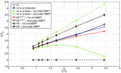
Figure 3: $E/E_{0}$ for the two-electron dot and for different methods as functions of $l_{0}/a_{B}^{*}$, where $l_{0}=\sqrt{\hbar/(m^{*}\omega)}$ is the characteristic dot length, $E_{0}=\hbar\omega$ is the single particle energy, and $a_{B}^{*}$ is the effective Bohr radius. Small values of $l_{0}/a_{B}^{*}$ correspond to stronger confinement and therefore a faster expected convergence rate of a perturbation expansion.

Finally the comparison with the pure one–electron wave functions in Fig. 2 clearly illustrates how much of an improvement it is to start the perturbation expansion from wave functions that already include some of the electron–electron interaction, especially for weaker potentials. This becomes even more clear in Fig. 3 where we present the results from Fig. 2 a) in another way. Here we have plotted $E_{Method}/E_{0}$ as functions of $l_{0}/a_{B}^{*}$ where $E_{0}=\hbar\omega$ is the single particle energy and $l_{0}=\sqrt{\hbar/(m^{*}\omega)}$ is the characteristic length of the dot. It demonstrates what an extraordinary improvement it is to start from Hartree–Fock compared to starting with the one–electron wave functions when doing second–order MBPT for low electron densities (high $l_{0}/a_{B}^{*}$). It also seems as there is a region where the Hartree-Fock starting point would yield a convergent perturbation expansion while taking the whole electron–electron interaction as the perturbation would not.

III.2 The six electron dot

In Fig. 4, a comparison between our HF and second–order MBPT calculations on the ground state of the six electron dot is made with a DFT calculation in the Local Spin Density Approximation(LSDA) as well as with a CI calculation, both by Reimann et al. Reimann et al. (2000). They performed their calculations for seven different electron densities here translated to potential strengths. Let us first focus on the results for the two highest densities, corresponding to a Wigner-Seitz radius $r_{s}=1.0a_{B}^{*}$ and $r_{s}=1.5a_{B}^{*}$ which translates to confinement strengths of $\hbar\omega\approx 7.58$ meV and $\approx 4.12$ meV respectively. The reason that we want to separate the comparison for those confinement strengths is that our Hartree-Fock calculations yield solutions with $\langle S^{2}\rangle>0$ for the weaker confinement strengths. A similar behavior was seen by Sloggett et al. Sloggett and Sushkov (2005) in their unrestricted HF calculations. Therefore the results for the weaker potentials overestimate the energy in a unphysical manner; compare the above discussion around Fig. 2 a). The CI-method however always yield $\langle S^{2}\rangle=0$ for the closed 6 electron shell and consequently a comparison with spin contaminated results would here, in some sense, be misleading. It should be emphasized that the spin contamination is a feature of our choice of starting point and not a problem with MBPT in itself.

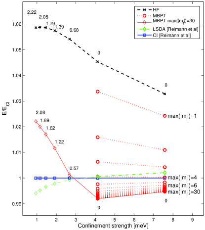
Figure 4: Comparison between our HF and second–order MBPT results for the six electron dot in the ground state with $M_{L}^{TOT}=0$ and $S_{z}^{TOT}=0$, with the LSDA and CI calculations by Reimann et alReimann et al. (2000). The second–order MBPT calculations include the full sum over the complete radial basis set (corresponding to all $n$-values) and with max$(|m_{\ell}|)=1,2,3,\ldots,30$ for the two strongest potentials. For clarity only the curves with max$(|m_{\ell}|)=1,4,6$ and $30$ have been labeled. The HF and the second–order MBPT with max$(|m_{\ell}|)=30$ curves are plotted for all potential strengths calculated by Reimann et al. Moreover, the values of $\langle S^{2}\rangle$ for the HF and the second–order MBPT with max$(|m_{\ell}|)=30$ have been plotted in the figure.

To make comparison easy all energies are normalized to the corresponding CI–value. The figure clearly illustrates, for the two stronger confinement strengths, that while the HF results overshoot the CI energy by between $3.5\%$ and $4.5\%$ the second order MBPT calculations improve the results significantly. Already for max$(|m_{\ell}|)=1$ the energy only overshoots the CI value with between $2.5\%$ and $3.5\%$ while the second–order MBPT energy for max$(m_{\ell})=4$ is almost spot on the CI energy. However, with max$(m_{\ell})=30$ the second–order MBPT gives somewhere between $0.5\%$ and $1\%$ lower energy than the CI calculation. We note that the CI calculation by Reimann et al. was made with a truncated basis set consisting of the states occupying the eight lowest harmonic oscillator shells. This means e.g. that their basis set includes only two states with $(|m_{\ell}|)=5$ and one with $(|m_{\ell}|)=6$. Within this space all possible six electron determinants were formed. After neglecting some determinants with a total energy larger than a chosen cutoff, the Hamiltonian matrix was constructed and diagonalized. Fig. 4 indicates that the basis set used in Ref. Reimann et al. (2000) was not saturated to the extent probed here, since almost all interactions with $|m_{\ell}|>4$ were neglected. According to Reimann et al. they used a maximum of $108$ $375$ Slater determinants while we, through perturbation theory, use a maximum of $980$ $366$ Slater determinants. The difference of our max$(|m_{\ell}|)=30$ results and their CI results are thus not unreasonable. Since Reimann et al. solved the full CI problem, the matrix to diagonalize is huge and it is, according to the authors, not feasible to use an even larger basis set. An alternative could be to include more basis functions, but restrict the excitations to single, doubles and perhaps triples. The domination of double excitations is well established in atomic calculations, see e.g. the discussion in Ref. Mårtensson-Pendrill et al. (1991). It should however be noted that the difference between the results concerns the fine details. Our converged results are less than one percent lower than those of Reimann et al. and when using approximately the same basis set as they did (max$(|m_{\ell}|)=4$) the difference between the results is virtually zero. Moreover, we see for the two strongest potentials the same trend as we saw in the two–electron case, namely that the HF, MBPT and CI results tend towards one another with increasing potential strength. This trend is not seen for the LSDA approach.

Finally, Fig. 4 shows, for the five weakest potentials, that our HF results get increasingly spin contaminated when the potential is weakened. Hereby the HF–approximation artificially lowers its energy and subsequently this leads to an overestimation of the second–order MBPT energies for these potential strengths. Surprisingly, however, the energy is never more than just above $2\%$ over the CI–results even when $\langle S^{2}\rangle>2$. Note also that MBPT improves the HF–value of $\langle S^{2}\rangle$ as it should.

III.3 Correlation in an external Magnetic Field

The behavior of quantum dots in an external magnetic field applied perpendicular to the dot has previously been examined many times both experimentally e.g.Tarucha et al. (1996); Kouwenhoven et al. (1997); Tarucha et al. (2000) and theoretically e.g Tarucha et al. (1996); Steffens et al. (1998); Szafran et al. (2003). The chemical potentials $\mu(N)=E(N)-E(N-1)$ plotted versus the magnetic field usually show a rich structure, including e.g. state switching and occupation of the lowest Landau band at high magnetic fields.

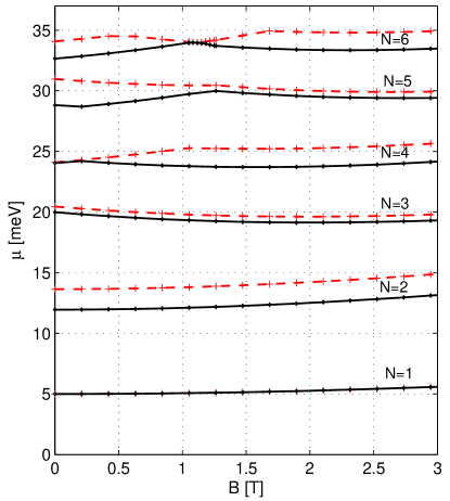
Figure 5: The chemical potentials for $N=1,2,$…$,6$ as functions of the external magnetic field according to HF (dashed curve) and second–order MBPT (full curve) calculations for the potential strength $\hbar\omega=5$ meV. Note the big difference between the two different models regarding the behavior of the chemical potentials when the magnetic field varies.

Fig.5 shows the chemical potentials for $N=1,2,\ldots,6$ as functions of the magnetic field according to our HF (dashed curves) and second–order MBPT with $-10\leq m_{\ell}\leq 10$ (full curves) calculations for the potential strength $\hbar\omega=5$ meV. We have here limited ourselves to the first six chemical potentials calculated at selected magnetic field strengths (shown by the marks in the figure). We emphasize again that our intention here is rather to test the capability of MBPT in the field of quantum dots than to provide a true description of the whole experimental situation. With increasing particle number MBPT naturally becomes more cumbersome, but magnetic field calculations are feasible at least up to $N=20$.

First note the significant difference between the HF and second–order MBPT results. Once again correlation proves to be extremely important in circular quantum dots. With our correlated results we also note a close resemblance both to the experimental work by Tarucha et al. Tarucha et al. (1996) and to the current spin-density calculation by Steffens et al. Steffens et al. (1998), made with the same potential and material parameters as used here. (Note that Ref. Steffens et al. (1998) defines the chemical potentials as $\mu(N)=E(N+1)-E(N)$, shifting all curves one unit in $N$). An example of the importance of correlation is the four-electron dot that switches state from $|\sum_{i=1}^{N}n_{i},|M_{L}|,S\rangle=|0,0,1\rangle$ to $|0,2,0\rangle$ at approximately $1$ T in the HF calculations and at approximately $0.2$ T in the correlated calculations. We want to emphasize that we have found the exact position of this switch to be very sensitive to the potential strength and to the value of $g^{*}$. The big difference concerning the magnetic field where this switch occurs can probably be attributed to the HF tendency to strongly favor spin-alignment. This is an effect originating from the inclusion of full exchange, but no correlation. Inclusion of second–order correlation energy cures this problem. Finally we note that the $N=5$ switch from $|0,1,\frac{1}{2}\rangle$ to $|0,4,\frac{1}{2}\rangle$ in our correlated calculations takes place somewhere around $1.2$ T which is also in agreement with both mentioned studies.

IV Results

IV.1 The addition energy spectra

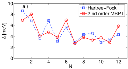
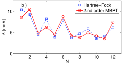
Figure 6: The ground state addition energy spectra for dots with $\hbar\omega=5$ meV (a) and $\hbar\omega=7$ meV (b). The squares (circles) represent the addition energy spectra according to HF (second–order MBPT). It is clear that the second–order MBPT–spectra imply closer resemblances to the experimental picture in TaruchaTarucha et al. (1996) than the HF–spectrum.

The so called addition energy spectra, with the addition energy defined as $\Delta(N)=E(N+1)-2E(N)+E(N-1)$, have been widely used to illustrate the shell structure in quantum dots. Main peaks at $N=2,6,12$ and $20$, indicating closed shells, and subpeaks at $N=4,9$ and $16$, due to maximized spin at half filled shells, have been interpreted as the signature for truly circular quantum dots Reimann et al. (1999). Experimental deviations from this behavior have been interpreted as being due to nonparabolicities of the confining potential or due to 3D–effectsMatagne et al. (2002). We here show that correlation effects in a true 2D harmonic potential can in fact generate an addition energy spectrum with similar deviations.

In this work we limit ourselves to the first three shells since it seems as the experimental situation is such that the validity of the 2D harmonic oscillator model becomes questionable with increasing particle numberMatagne et al. (2002). Calculations of dots with larger $N$ could, however, readily be made with our procedure. The addition energy spectra are produced with $-10\leq m_{\ell}\leq 10$. The filling order for the first six electrons is straight forward. When the seventh electron is added to the dot the third shell starts to fill. With a pure circular harmonic oscillator potential and no electron-electron interaction the $\mid 0,\pm 2,\pm\frac{1}{2}\rangle$ and $\mid 1,0,\pm\frac{1}{2}\rangle$ one-particle states are completely degenerate. This degeneracy is lifted by the electron-electron interaction, but not more than that the energies have to be studied in detail in order to determine the filling order. Similar conclusions, that the filling order is very sensitive to small perturbations, have been drawn by Matagne et al.Matagne et al. (2002), who studied the influence of non-harmonic 3D effects. Our focus is instead the detailed description of the electron-electron interaction. For $N=7-11$ we have thus calculated all third shell configurations, and for each configuration considered the maximum spin. The results are found in Table 1. For each number of electrons we can identify a ground state, which sometimes differs between HF and MBPT. These ground states are used when creating Fig. 6a) and b). The energy gap to the first excited state is sometimes very small and the possibility of alternative filling orders will be discussed in the next section.

Fig. 6a) and Fig. 6b) thus show the ground state addition energy spectra up to $N=12$ according to the Hartree-Fock model as well as to second–order MBPT for $\hbar\omega=5$ and $7$ meV. Note first the big difference between the HF and MBPT spectra. These figures clearly illustrate how important correlation effects are in these systems. Admittedly the HF–spectra show peaks at $N=4,6,9$ and $12$ but the relative size of the addition energy between closed and half–filled shells is not consistent with the experimental pictureTarucha et al. (1996); Matagne et al. (2002). The second–order MBPT–spectra have in contrast clear main peaks at $N=2,6$ and $12$, indicating closed shells, and a $N=4$ subpeak indicating maximized spin for the half filled shell. For the $\hbar\omega=7$ meV spectrum the subpeak at $N=9$ is also clear but for the $\hbar\omega=5$ meV spectrum the subpeak at $N=9$ is substituted by subpeaks at $N=8$ and $10$. The behavior of the addition energy spectra in this, the third shell, will be discussed in detail below.

Table 1: Energy of the ground and third shell excited state for 7–11 electron dots with $\hbar\omega=5$ and $7$ meV. The notation $(\sum_{i=1}^{N}n,|M_{L}|,S)$ to label the state is used. The ground state energy according to Hartree–Fock (HF energy) and to HF + second–order MBPT (Correlated energy) and for respective N and potential strength is marked in bold.

# $e^{-}$		$\hbar\omega=5$ meV				$\hbar\omega=7$ meV
7	State	$(0,2,\frac{1}{2})$		$(1,0,\frac{1}{2})$		$(0,2,\frac{1}{2})$		$(1,0,\frac{1}{2})$
	HF energy [meV]	168.02		168.67		$\mathbf{215.80}$		$216.58$
	Correlated energy [meV]	162.08		162.15		$\mathbf{208.96}$		$209.52$
8	State	$(0,0,1)$	$(0,4,0)$	$(1,2,1)$	$(2,0,0)$	$(0,0,1)$	$(0,4,0)$	$(1,2,1)$	$(2,0,0)$
	HF energy [meV]	210.69	212.33	211.66	214.00	$\mathbf{270.66}$	272.20	271.51	274.32
	Correlated energy [meV]	205.23	204.40	204.66	205.02	263.82	$\mathbf{263.70}$	263.85	264.65
9	State	$(1,0,\frac{3}{2})$	$(0,2,\frac{1}{2})$	$(1,4,\frac{1}{2})$	$(2,2,\frac{1}{2})$	$(1,0,\frac{3}{2})$	$(0,2,\frac{1}{2})$	$(1,4,\frac{1}{2})$	$(2,2,\frac{1}{2})$
	HF energy [meV]	257.69	259.24	259.28	260.56	$\mathbf{330.25}$	332.17	332.14	333.64
	Correlated energy [meV]	250.54	251.35	250.95	251.00	$\mathbf{322.27}$	322.81	323.06	323.37
10	State	$(1,2,1)$	$(0,0,0)$	$(2,0,1)$	$(2,4,0)$	$(1,2,1)$	$(0,0,0)$	$(2,0,1)$	$(2,4,0)$
	HF energy [meV]	309.27	310.64	310.17	311.06	$\mathbf{395.72}$	397.20	396.73	397.78
	Correlated energy [meV]	300.49	300.00	300.25	300.52	385.92	$\mathbf{385.76}$	386.06	386.49
11	State	$(1,0,\frac{1}{2})$		$(2,2,\frac{1}{2})$		$(1,0,\frac{1}{2})$		$(2,2,\frac{1}{2})$
	HF energy [meV]	363.72		364.49		$\mathbf{464.77}$		465.57
	Correlated energy [meV]	353.66		353.19		453.47		$\mathbf{453.43}$

Table 2: Expectation values of $S^{2}$ for the cases where correlation switches ground states in the third shell. The state labeled “Ground State” is the ground state according to second–order MBPT while the state labeled “Excited State” is the ground state according to Hartree-Fock but an excited state according to second–order MBPT.

# e-		$\hbar\omega=5meV$				$\hbar\omega=7meV$
		Ground State		Excited state		Ground State		Excited state
		E [meV]	$\langle S^{2}\rangle$	E [meV]	$\langle S^{2}\rangle$	E [meV]	$\langle S^{2}\rangle$	E [meV]	$\langle S^{2}\rangle$
$8$	HF	212.33	0.00	210.69	2.70	272.20	0.00	270.66	2.30
	$2^{nd}$–ord MBPT	204.40	0.00	205.23	2.58	263.70	0.00	263.82	2.22
	Exact		0		2		0		2
$10$	HF	310.64	0.00	309.27	2.21	397.20	0.00	395.72	2.08
	$2^{nd}$–ord MBPT	300.00	0.00	300.49	2.15	385.76	0.00	385.92	2.05
	Exact		0		2		0		2
$11$	HF	364.49	0.77	363.72	0.99	465.57	0.758	464.77	0.82
	$2^{nd}$–ord MBPT	353.19	0.76	353.66	0.93	453.43	0.755	453.47	0.79
	Exact		0.75		0.75		0.75		0.75

IV.1.1 Filling of the third shell

The filling of the third shell has previously been examined by Matagne et al. Matagne et al. (2002) both experimentally and theoretically. In their theoretical description they use a 3D DFT model with the possibility to introduce a nonharmonic perturbation that can change the ground states in the third shell and thereby alter the addition energy spectra. They then compare their theoretical description with different experimental addition energy spectra and argue how large deviation from the circular shape they have in the different experimental setups. They conclude that a clear dip at $N=7$ followed by a peak at $N=8$ or $9$ is a signature of maximized spin at half filled shell and that a dip at $N=7$ and the filling sequence

$$\left|\sum_{i=7}^{N}n^{i},|\sum_{i=7}^{N}m_{\ell}^{i}|,S\right\rangle=\,\mid 0,2,\frac{1}{2}\rangle\Rightarrow\mid 0,0,1\rangle\Rightarrow$$

$$\mid 1,0,\frac{3}{2}\rangle\Rightarrow\mid 1,2,1\rangle\Rightarrow\mid 1,0,\frac{1}{2}\rangle\Rightarrow\mid 2,0,0\rangle$$ (16)

for the six electrons to enter the third shell is a signature of a “near ideal artificial atom”. This is also the filling sequence we find using the HF- approximation. As seen in Fig. 6a) and b) there is then indeed also a dip at $N=7$ and a peak at $N=9$. The dip at $N=7$ is further supported by the DFT calculation by Reimann et al. Reimann et al. (1999). In contrast the experiment by Tarucha et al.Tarucha et al. (1996) did not show the $N=7$ dip. In Ref. Matagne et al. (2002) this is explained by deviations from circular symmetry for the specific dot used in Ref. Tarucha et al. (1996). As will be seen below our many-body calculations give in several cases different ground states and thus favor a different filling order than Eq.IV.1.1.

Table 1 shows the ground state and excited states energies of the third shell according to HF and second–order MBPT for $\hbar\omega=5$ meV and $\hbar\omega=7$ meV. Notice that the different methods yield different ground states for the $8,10$ and $11$–electron systems although both potential strengths yield the same ground states. Note also the small excitation gap between the correlated ground and first excited state that occurs in some cases. For example between the $\mid 0,2,\frac{1}{2}\rangle$ and $\mid 1,0,\frac{1}{2}\rangle$ seven-electron states in the $\hbar\omega=5$ meV dot the energy difference is $0.07$ meV, between the $\mid 0,0,1\rangle$ and $\mid 0,4,0\rangle$ eight-electron state in the $\hbar\omega=7$ meV dot the energy difference is $0.12$ meV and between the $\mid 1,0,\frac{1}{2}\rangle$ and $\mid 2,2,\frac{1}{2}\rangle$ eleven-electron states in the $\hbar\omega=7$ meV dot the energy difference is only $0.04$ meV. The $(1,0,\frac{3}{2})$ state at $N=9$ seems, however, relatively stable for both potential strengths with excitation gaps of $0.41$ and $0.54$ meV. Surprisingly for both the $\hbar\omega=5$ and $7$ meV the calculations including correlations indicate the ground state third shell filling sequence

$$\mid~{}0,2,\frac{1}{2}\rangle\Rightarrow\mid~{}0,4,0\rangle\Rightarrow\mid~{}1,0,\frac{3}{2}\rangle\Rightarrow$$

$$\mid~{}0,0,0\rangle\Rightarrow\mid~{}2,2,\frac{1}{2}\rangle\Rightarrow\mid~{}2,0,0\rangle$$ (17)

for $N=7-12$. Note that this sequence implies a spin-flip of the electrons already in the dot when the ninth and tenth electrons are added. Only the seven-electron dot and the nine-electron dot here have the same ground state as in HF (whose filling sequence coincides with that preferred in Ref Matagne et al. (2002)). Matagne et al. also discuss that the behavior of the dot examined in Ref. Tarucha et al. (1996) for small magnetic fields implies the sequence

$$\mid~{}0,2,\frac{1}{2}\rangle\Rightarrow\mid~{}0,4,0\rangle\Rightarrow\mid~{}1,2,\frac{1}{2}\rangle\Rightarrow$$

$$\mid~{}0,0,0\rangle\Rightarrow\mid~{}1,0,\frac{1}{2}\rangle\Rightarrow\mid~{}2,0,0\rangle,$$ (18)

but tend to attribute this to deviations from circular shape. This filling sequence is indeed much closer to the ground states we have obtained with a perfect circular potential. This indicates the possibility that many-body effects usually neglected could have an effect similar to that of imperfections in the dot construction. We note in passing that Sloggett and Sushkov Sloggett and Sushkov (2005) support our finding of a spin-zero ground-state for ten electrons, although their calculation was done with a stronger potential. The different configurations for nine electrons in Eq. IV.1.1 and Eq. IV.1.1 can be due to the fact that the experimental situation favors population of an excited state since population of the ground state would require a spin flip. However, if we produce a spectrum with this filling sequence, we get a large dip at $N=9$. Similarly, when the eleventh electron is injected, the population of our ground state would require a configuration change of the electrons already in the dot.

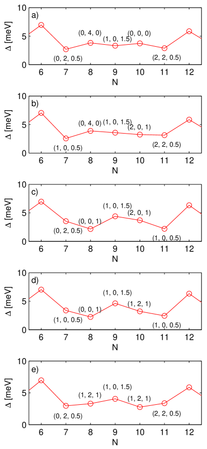
Figure 7: Ground state, a), and selected excited state, b)-e), addition energy spectra for $\hbar\omega=5$ meV according to second–order MBPT. The notation $(\sum_{i=7}^{N}n^{i},|\sum_{i=7}^{N}m_{\ell}^{i}|,S)$ to label the states is used. Note the big differences between the different spectra. For example the ground state spectrum, a), has peaks at $N=8,10$ while spectrum b) has a peak at $N=8$ and the rest have a peak at $N=9$. That is, even if the spin is maximized at half filled shell ($N=9$) there is not always a peak there as seen in subfigure a) and b). Subfigure e) resembles the experimental results of Ref. Matagne et al. (2002) best with dips at $N=7$ and $10$ and a peak at $N=9$. Moreover, combining the addition energies for $N=6,7,8$ of sequence c) or d) with the addition energies for $N=10,11,12$ of sequence e) would give a spectrum that closely resembles the experimental situation in Ref. Tarucha et al. (1996) with dips at $N=8$ and $10$ and a peak at $N=9$.

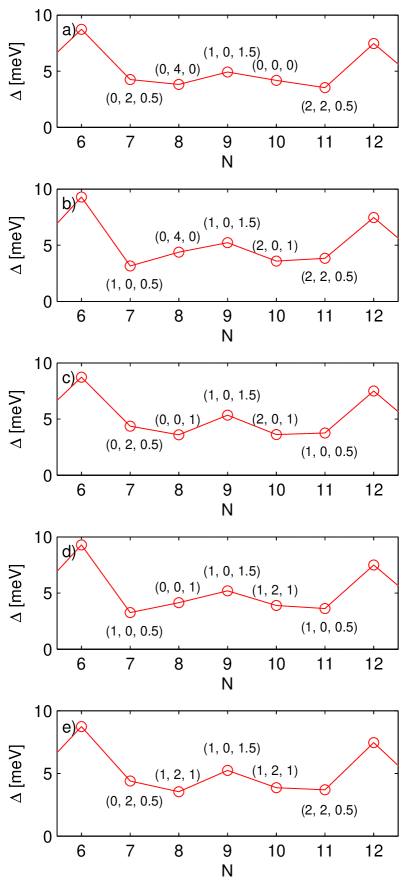
Figure 8: Ground state, a), and selected excited state, b)-e), addition energy spectra for $\hbar\omega=7$ meV according to second–order MBPT. The notation $(\sum_{i=7}^{N}n^{i},|\sum_{i=7}^{N}m_{\ell}^{i}|,S)$ to label the states is used. Note the big differences between the different spectra. Note also that all spectra have peaks at $N=9$. Even though the ground state spectra for $N=7,8$ and $9$ resemble the experimental results of Ref. Tarucha et al. (1996), the dip at $N=11$ is uncharacteristic when compared with the experimental results of Ref. Tarucha et al. (1996) and Ref. Matagne et al. (2002). Subfigure b) resembles the experimental result in Ref. Matagne et al. (2002) the most with a peak at $N=9$ and dips at $N=7$ and $10$ while subfigure c) resembles the experimental results of Ref. Tarucha et al. (1996) the most with a peak at $N=9$ and dips at $N=8$ and $10$.

In Fig. 7 and Fig. 8 addition energy spectra are shown assuming different filling orders for $5$ meV and $7$ meV, respectively. In each figure the calculated ground state filling sequence is shown in the uppermost panel, labeled a), and then the other panels, e) – f), show selected excited state filling sequences. Note that even though the same filling sequences are used in Fig. 7 and Fig. 8 the addition energy spectra differ between these rather close potential strengths. We can thus conclude that a given filling sequence does not yield a unique addition energy spectra since the relative energies of the ground and excited states are very sensitive to the exact form of the potential. Furthermore we agree with Matagne et al. Matagne et al. (2002) that full spin alignment for the nine-electron ground state does not guarantee a peak in the addition energy spectrum as seen in Fig. 7 a) and b). Moreover we see that the spectra that resemble the experimental one in Fig. 3a) of Ref. Matagne et al. (2002) (a clear dip at $N=7$ and $10$ and a clear peak at $N=9$) are Fig. 7e) and Fig. 8b). Finally we see that Fig. 8c) resembles the experimental situation in Ref. Tarucha et al. (1996) (dips at $N=8$ and $10$ with a peak at $N=9$) the most. We certainly do not claim that these filling sequences are those really obtained in the mentioned experiments. However, we want to stress that great care must be taken when conclusions are drawn from comparisons between theoretical and experimental addition energy spectra.

IV.1.2 Spin contamination in the third shell

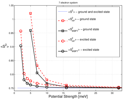
Figure 9: $\langle S^{2}\rangle$ according to Hartree-Fock and second–order MBPT calculations as functions of the potential strength for the 7 electron ground and excited state.

Fig. 9 shows the expectation value of the total spin, $\langle S^{2}\rangle$, according to Hartree-Fock and second–order MBPT calculations as functions of the potential strength for the 7 electron ground and excited state. The figure depicts the drastic onset of spin contamination for weak potentials. While especially the correlated results, but also the HF–results, converge towards the correct value for potentials $\geq 10$ meV the situation is worse for weaker potentials. We see that for the ground state the examined confinement strengths in this article ($\hbar\omega=5$ or $7$ meV) lie on the onset of the spin density wave. It is hard to say how much this spin contamination affects the energy values but when compared with the conclusions drawn from Fig. 2 and 4, the energy should not be overestimated with more than a couple of percent due to spin contamination. For the excited state the spin contamination is so small (for the $5$ and $7$ meV calculations) that it should not affect the conclusions from this work. Moreover we see that, as expected, correlation improves the value of $\langle S^{2}\rangle$.

Table 2 presents the spin contamination for the systems in the third shell where correlation switched the ground state, namely the 8, 10 and 11 electron systems. We see that the ground states, according to our correlated results, are not spin contaminated to any relevant magnitude. All the excited states are however spin contaminated. As shown in Fig. 4, spin contamination can lower the HF energy and raise the second–order MBPT energy. The ground state energy switches could thus be an artifact of our starting point. Energywise however the correlated energies should lie much closer to the true values than the HF–energies.

V Conclusions

We have shown that the addition of second–order correlation improves the Hartree-Fock description of two-dimensional few-electron quantum dots significantly. Our results indicate that details in the addition energy spectra often attributed to 3D–effects or deviations from circular symmetry, are indeed sensitive to the detailed description of electron correlation on more or less the same level. Without precise knowledge of the many-body effects far reaching conclusions about dot properties from the addition energy spectra might not be correct.

As a next step we want to include pair-correlation to higher orders to be able to determine energies with quantitative errors below 0.1meV. We will then use several different starting potentials to be able to address also weak confining potentials where the Hartree–Fock starting point fails.