Discretized vs. continuous models of p-wave interacting fermions in 1D

Abstract

We present a general mapping between continuous and lattice models of Bose- and Fermi-gases in one dimension, interacting via local two-body interactions. For $s$-wave interacting bosons we arrive at the Bose-Hubbard model in the weakly interacting, low density regime. The dual problem of $p$-wave interacting fermions is mapped to the spin-1/2 XXZ model close to the critical point in the highly polarized regime. The mappings are shown to be optimal in the sense that they produce the least error possible for a given discretization length. As an application we examine the ground state of a interacting Fermi gas in a harmonic trap, calculating numerically real-space and momentum-space distributions as well as two-particle correlations. In the analytically known limits the convergence of the results of the lattice model to the continuous one is shown.

I introduction

Triggered by the recent successes in the experimental realization of strongly interacting atomic quantum gases in one spatial dimensional (1D) Kinoshita et al. (2004); Paredes et al. (2004); Gunter et al. (2005); Hofferberth et al. (2007); Haller et al. (2009) there is an increasing interest in the theoretical description of these systems beyond the mean field level. Model hamiltonians describing homogeneous 1D quantum gases with contact interaction are often integrable by means of Bethe Ansatz Bethe (1931); Lieb and Liniger (1963); Korepin et al. (1993); Gaudin (1983). In practice, however, only a small number of quantities can actually be obtained from Bethe Ansatz or explicit calculations are restricted to a small number of particles. Properties associated with low energy or long wavelength excitations can, to very good approximation, be described by bosonization techniques Giamarchi (2003). For more general problems one has to rely on numerical techniques such as the density matrix renormalization group (DMRG) White (1992); Schollwöck (2005) or the related time evolving block decimation (TEBD) Vidal (2003, 2004). Both have originally been developed for lattice models and thus in order to apply them to continuous systems requires a proper mapping between the true continuum model and a lattice approximation. In fact any numerical technique describing a continuos system relies on some sort of discretization. Here we consider massive bosonic or fermionic particles with contact interactions. Only two types of contact interaction potentials are allowed for identical, nonrelativistic particles, representing either bosons with s-wave interactions or fermions with p-wave interactions. Both systems are dual and can be mapped onto each other by the well-known boson-fermion mapping Girardeau (1960); Cheon and Shigehara (1999). A proper discretization of 1D bosons with s-wave interaction is straight forward and has been used quite successfully to calculate ground-state Schmidt and Fleischhauer (2007), finite temperature Schmidt et al. (2005), as well as dynamical problems Muth et al. (2009) for trapped 1D gases. For p-wave interacting fermions a similar, straight forward discretization fails however, as can be seen when comparing numerical results using such a model with those obtained from the bosonic Hamiltonian after the boson-fermion mapping. Using a general approach to quantum gases in 1D with contact interaction Schmidt (2009) we here derive a proper mapping between continuous model and lattice approximation. We show in particular that p-wave interacting fermions are mapped to the critical spin 1/2 XXZ model. By virtue of the boson-fermion mapping the same can be done for s-wave interacting bosons, thus maintaining integrability in the map between continuous and discretized models. As an application we calculate the real-space and momentum-space densities of the ground state of a p-wave interacting Fermi gas in a harmonic trap, as well as local and non-local two particle correlations in real space. To prove the validity of the discretized fermion model we compare the numerical results with those obtained from the dual bosonic model as well as with Bethe ansatz solutions when available.

II 1D quantum gases with general contact interactions

We here consider quantum gases, that are fully described by their two particle Hamiltonian, i.e., the Hamiltonian is a sum of the form

$$H=-\frac{1}{2}\sum_{j}\partial_{x_{j}}^{2}+\sum_{i<j}V(x_{i}-x_{j}).$$ (1)

Additionally we require that the true interaction potential can be approximated by a local pseudo-potential, i.e. it vanishes for $x_{i}\neq x_{j}$. Since we are in one dimension, this leads to the exact integrability of these models in the case of translational invariance Lieb and Liniger (1963) using coordinate Bethe ansatz Bethe (1931); Gaudin (1983).

For deriving a discretized Hamiltonian, it is sufficient to consider the relative wave function $\phi(x=x_{1}-x_{2})$ of just two particles. The Hamiltonian then reads

$$H=-\partial_{x}^{2}+V(x)$$ (2)

where we have dropped the term corresponding to the freely evolving center of mass.

The continuous two-particle case has been analyzed by Cheon and Shigehara Cheon and Shigehara (1998, 1999). The local pseudo-potential $V$ is fully described by a boundary condition on $\phi$ at $x=0$: Since $\phi$ fulfills the free Schrödinger equation away from $0$, it must have a discontinuity at the origin as an effect of the interaction. Thus we see that

$$\partial_{x}^{2}\phi(x)=\left\{\begin{array}[]{cl}\phi^{\prime\prime}(x)&x\neq 0\\ \delta(x)\left[\phi^{\prime}(0^{+})-\phi^{\prime}(0^{-})\right]+&\\ \quad+\ \delta^{\prime}(x)\left[\phi(0^{+})-\phi(0^{-})\right]&x=0.\end{array}\right.$$ (3)

In the case of distinguishable or spinful Girardeau and Olshanii (2004) particles both singular terms contribute. Due to symmetry, the term proportional to the delta function $\delta$ can only be nonzero for bosons, while the $\delta^{\prime}$ term exists only for fermions. I.e. we have for bosons

$$\partial_{x}^{2}\phi(x)=\left\{\begin{array}[]{cl}\phi^{\prime\prime}(x)&x\neq 0\\ 2\delta(x)\phi^{\prime}(0)&x=0.\end{array}\right.$$ (4)

and for fermions

$$\partial_{x}^{2}\phi(x)=\left\{\begin{array}[]{cl}\phi^{\prime\prime}(x)&x\neq 0\\ \ 2\delta^{\prime}(x)\phi(0)&x=0.\end{array}\right.$$ (5)

In order to get proper eigenstates (i.e. without any singular contribution), the pseudo-potential $V$ acting on the wave-function must absorb the singular contributions from the kinetic energy. Thus the only possible form of a local pseudo-potential for bosons is $V_{B}\phi=g_{\text{B}}\delta(x)\phi(0)$, while that for fermions reads $V_{F}\phi=-g_{\text{F}}\delta^{\prime}(x)\phi^{\prime}(0)$. Note that $\phi$ ($\phi^{\prime}$) is continuous at 0 for bosons (fermions). These two possibilities represent the well known cases, where the particle interact either by s-wave scattering only or by p-wave scattering only, and the interaction strength corresponds to the scattering length, respectively scattering volume, which are the only free parameters left.

Since all wave functions must have the respective symmetry, we can restrict ourselves in the following to the $x>0$ sector. We will write $\phi(0)$ for $\lim_{x\rightarrow 0^{+}}\phi(x)$ and $\phi^{\prime}(0)$ for $\lim_{x\rightarrow 0^{+}}\phi^{\prime}(x)$. The above shows that $V$ imposes a boundary condition on every proper wave function:

$$\begin{array}[]{ll}\phi^{\prime}(0)=\frac{g_{\text{B}}}{2}\phi(0)&\quad\textrm{bosons},\cr\phi^{\prime}(0)=-\frac{2}{g_{\text{F}}}\phi(0)&\quad\textrm{fermions}.\end{array}$$ (6)

Eqs.(3) and (6) reveal a one-to-one mapping between the two cases, i.e., every solution for the bosonic problem yields a solution for the fermionic problem with $g_{\text{B}}=-4/g_{\text{F}}$ by symmetrizing the wave function and vice versa.

At this point we emphasize, that boundary conditions of the above form are the only ones that are equivalent to a local potential Seba (1986); Cheon and Shigehara (1998). While boundary conditions involving higher order derivatives can be taken into account to describe experimental realizations using cold gases in quasi 1D traps Imambekov et al. (2009), the necessarily require finite range potentials and cannot be described fully by local pseudo-potentials.

III discretization

The treatment of continuous gases in one-dimension using numerical techniques requires a proper discretization. That is we approximate the two-particle wave function $\phi(x)\in L^{2}(\mathbb{R})$ by a complex number $\phi_{j}\in\ell^{2}(\mathbb{Z})$, where the integer index $j$ describes the discretized relative coordinate $x=x_{1}-x_{2}$. We interpret $|\phi_{j}^{2}|$ as the probability to find the two particles between $(j-\frac{1}{2})\Delta x$ and $(j+\frac{1}{2})\Delta x$. In order to apply numerical methods such as DMRG or TEBD Vidal (2004, 2003) efficiently, it is favorable to have local or at most nearest neighbor interactions in the lattice approximation of the continuous model. It will turn out, that the above systems can all be discretized using such nearest neighbor interactions only.

We start with the kinetic term, that can be approximated by

$$\partial_{x}^{2}\mapsto\frac{\phi_{j-1}-2\phi_{j}+\phi_{j+1}}{\Delta x^{2}}.$$ (7)

In what follows, we will derive two distinct discretizations: first for the bosons, where we allow for double occupied lattice sites and can therefore use on-site interactions to reproduce the boundary conditions (6), and then for fermions, where double occupation is forbidden by the Pauli principle and interactions between neighbors are necessary in the lattice model. Note however, that both descriptions are equivalent due to the Bose Fermi mapping in the continuum limit.

III.1 bosonic mapping

In the lattice approximation the kinetic-energy term, Eq.(3) reads

$$\partial_{x}^{2}\phi(x)=\left\{\begin{array}[]{cl}\frac{\phi_{j-1}-2\phi_{j}+\phi_{j+1}}{\Delta x^{2}}&j>0\\ \frac{2(\phi_{1}-\phi_{0})}{\Delta x^{2}}&j=0\end{array}\right.$$ (8)

Thus assuming a local contact interaction only, we find for the bosons

$$(H\phi)_{j}=\left\{\begin{array}[]{cl}-\frac{\phi_{j-1}-2\phi_{j}+\phi_{j+1}}{\Delta x^{2}}&j>0\\ U\phi_{0}-\frac{2\phi_{1}-2\phi_{0}}{\Delta x^{2}}&j=0\end{array}\right..$$ (9)

In order to determine the value of $U$, we assume, that it can be expressed as a series in $\Delta x$ and evaluate the stationary Schrödinger equation $(H\phi)_{j}-E\phi_{j}=0$ at $j=0$. Reexpressing $\phi_{1}$ in terms of $\phi(0)$ by means of the discretized version of the contact condition (6)

$$\phi_{1}=\phi(0)+\Delta x\underbrace{\phi^{\prime}(0)}_{=\frac{g_{\text{B}}}{2}\phi(0)}+\frac{\Delta x^{2}}{2}\underbrace{\phi^{\prime\prime}(0)}_{=-E\phi(0)}+\dots,$$ (10)

we arrive at

$$0 = (H\phi)_{j=0}-E\phi_{j=0}$$

$$= U\phi(0)+\frac{2\phi(0)}{\Delta x^{2}}-E\phi(0)-\frac{2}{\Delta x^{2}}\times$$

$$\times \left(\phi(0)+\Delta x\frac{g_{\text{B}}}{2}\phi(0)-\frac{1}{2}\Delta x^{2}E\phi(0)+\mathcal{O}(\Delta x^{3})\right).$$

Equating orders gives

$$U=\frac{g_{\text{B}}}{\Delta x}+\mathcal{O}(\Delta x).$$ (12)

The constant term vanishes, since $-\partial_{x}^{2}\phi=E\phi$ for any eigenstate. The higher orders $\mathcal{O}(\Delta x)$ contain $E$ and would thus not be independent on the eigenvalue. This is perfectly consistent, since discretizations will only work a long as the lattice spacing is much smaller than all relevant (wave) lengths in the system. Thus the lowest order in (12) is already optimal. There are no higher order corrections possible for a general state.

We can now easily write down the corresponding many particle Hamiltonian for the case of indistinguishable bosons in absolute coordinates, represented by an integer index $i$ and in second quantization:

$$H=\sum_{i}\left[-J(a_{i}^{\dagger}a_{i+1}+h.a.)+\frac{U}{2}a_{i}^{\dagger}a_{i}^{\dagger}a_{i}a_{i}+V_{i}a^{\dagger}_{i}a_{i}\right].$$ (13)

Here $a_{i}$ is the bosonic annihilator at site $i$ and $V_{i}$ introduces an additional external potential in the obvious way. So not surprisingly we have arrived at the Bose-Hubbard Hamiltonian as a lattice approximation to 1D bosons with s-wave interaction. Since $\Delta x$ must be smaller than all relevant length scales, we are however in the low-filling and weak-interaction limits $U\ll J=\frac{1}{2\Delta x^{2}}$ . This does of course not imply that the corresponding Lieb-Liniger gas is in the weakly interacting regime. This result might seem trivial, since we can also directly get it by substituting the field operator in the continuous model: $\Psi(j\Delta x)\mapsto\frac{a_{j}}{\sqrt{\Delta x}}$ Schmidt and Fleischhauer (2007). However, this simple and naive discretization does not work in the fermionic case we are going to discuss now.

III.2 fermionic mapping

For fermions the kinetic-energy term, Eq.(3) reads in lattice approximation

$$\partial_{x}^{2}\phi(x)=\left\{\begin{array}[]{cl}\frac{\phi_{j-1}-2\phi_{j}+\phi_{j+1}}{\Delta x^{2}}&j>1\\ \frac{\phi_{2}-2\phi_{1}}{\Delta x^{2}}&j=1\\ 0&j=0\end{array}\right.$$ (14)

Due to the anti-symmetry of the wave-function $\phi_{0}$ must vanish, i.e. the simplest way interactions come into the lattice model is for nearest neighbors. Thus we write for the Hamiltonian

$$(H\phi)_{j}=\left\{\begin{array}[]{cl}-\frac{\phi_{j-1}-2\phi_{j}+\phi_{j+1}}{\Delta x^{2}}&j>1\\ B\phi_{1}-\frac{\phi_{2}-2\phi_{1}}{\Delta x^{2}}&j=1\\ 0&j=0\end{array}\right.$$ (15)

To obtain the value of $B$ we proceed as in the case of bosons. As will be seen later on it is most convenient to expand $B$ in a series in the following way:

$$\frac{1}{B}=\Delta x^{2}\left(B^{(2)}+\Delta xB^{(3)}+\mathcal{O}(\Delta x^{2})\right).$$ (16)

Now the stationary Schrödinger equation for $j=1$ yields

$$0=1-\frac{2}{g_{\text{F}}}\Delta x-\frac{\Delta x^{2}}{2}E+\mathcal{O}(\Delta x^{3})+$$ (17)

$$+\left(B^{(2)}+\Delta xB^{(3)}+{\Delta x^{2}}B^{(4)}+\mathcal{O}(\Delta x^{2})\right)\left[1+\mathcal{O}(\Delta x^{3})\right].$$

Equating orders results in

$$B^{(2)}=-1,\quad B^{(3)}=\frac{2}{g_{\text{F}}},\quad B^{(4)}=\frac{1}{2}E.$$ (18)

Note that his time the interaction appears only in the second lowest order, which can not be described by a simple substitution formula. The next higher order contained in $\mathcal{O}(\Delta x^{2})$ does not vanish, but depends again on the energy as expected. If we had chosen a straightforward expansion of $B$ instead of (16), the next order after the one that introduces the interaction would have contained again the interaction parameter:

$$B=-\frac{1}{\Delta x^{2}}-\frac{2}{g_{F}\Delta x}-\frac{4}{g_{F}^{2}}+\frac{E}{2}+\mathcal{O}(\Delta x).$$ (19)

Neglecting this term would therefore introduce a larger error than in the chosen expansion (16). In fact the low energy scattering properties would be reproduced only to one order less. For the bosons this problem did not occur (12). From (16) we read that the optimal result in the fermionic case is

$$B=-\frac{1}{\Delta x^{2}}\left(\frac{1}{1-\frac{2\Delta x}{g_{\text{F}}}}\right).$$ (20)

The corresponding many-body Hamiltonian for indistinguishable fermions reads

$$H=\sum_{i}\left[-J(c_{i}^{\dagger}c_{i+1}+h.a.)+Bc_{i}^{\dagger}c_{i}c_{i+1}^{\dagger}c_{i+1}+V_{i}c_{i}^{\dagger}c^{\dagger}_{i}\right],$$ (21)

where now $c_{i}$ is a fermionic annihilator at site $i$. Eq. (21) describes spin polarized lattice fermions with hopping $J$ and nearest-neighbor interaction $B$. In contrast to the bosonic case, Eq.(18), where the correct discretized model could be obtained from the continuum Hamiltonian just by setting $\Psi(x)\rightarrow a_{i}/\sqrt{\Delta x}$, we now see from (21) and (20) that a similar naive and straight-forward discretization fails in the case of $p$-wave interacting fermions.

The failure of a naive discretization of the fermionic Hamiltonian becomes transparent if we map this model to that of a spin lattice: Using the Jordan-Wigner transformation

$$\sigma_{i}^{+}=\exp\Bigl{\{}i\pi\sum_{l<i}c_{l}^{\dagger}c_{l}\Bigr{\}}\,c_{i},\qquad\sigma_{i}^{z}=2c_{i}^{\dagger}c_{i}-1$$ (22)

(21) can be mapped to the spin-1/2 XXZ model in an external magnetic field

$$H = \sum_{i}\Big{\{}-\frac{1}{4\Delta x^{2}}\big{(}\sigma_{i}^{x}\sigma_{i+1}^{x}+\sigma_{i}^{y}\sigma_{i+1}^{y}+$$ (23)

$$+ \Delta(\sigma_{i}^{z}+1)(\sigma_{i+1}^{z}+1)\big{)}+V_{i}\sigma_{i}^{z}\Big{\}},$$

where the anisotropy parameter defining the XXZ model is $\Delta=-1/[1-\frac{2\Delta x}{g_{\text{F}}}]$.

There is an easy way to see that these mappings are quite physical by considering the ground states: The repulsive Bose gas ($g_{\text{B}}>0$) maps to the repulsive ($U>0$) Bose-Hubbard model in the super fluid, low filling regime, which has an obviously gas like ground state. The same is true for the corresponding attractively interacting ($g_{\text{F}}<0$) Fermi gas, which maps to the ferromagnetic XXZ model which, due to the specific form of the interaction parameter in the discretized fermion model, Eq.(20), is always in the critical regime close to the transition point ($\Delta^{\underrightarrow{\Delta x\rightarrow 0}}-1^{+})$. A naive discretization would have lead to an anisotropy parameter that could cross the border to the gapped phase, which is clearly unphysical.

In the attractive Bose gas, bound states emerge, that lead to a collapse of the ground state as it is of course also true in the Bose Hubbard model for $U<0$. On the fermionic side, this collapse can be also observed, as for $\Delta<-1$ the XXZ model has a ferromagnetically ordered ground state, which leads to phase separation in the case of fixed magnetization.

Note that we call the Fermi gas repulsively interacting if $g_{\text{F}}>0$, although $B$ is negative in this case as well, and although there exist bound states, who’s binding energy actually diverges as $g_{\text{F}}\rightarrow 0^{+}$, as is immediately clear from the Bose Fermi mapping in the continuous case.

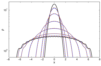
Figure 1: (Color online) Local density distribution of the interacting Fermi or Bose gas. The (orange) dashed lines show results obtained by Bose-Fermi mapping and solving the Bose Hubbard lattice model, the (blue) continuous lines correspond to the XXZ discretization. The interaction strength $g_{\text{F}}$ is $-51.2,-12.8,-3.2,-0.8,-0.2,-0.05$ from the narrow to the broad distributions. The solid black lines show the limiting cases of free fermions (broad) and infinitely strong interacting fermions (narrow, corresponds to free bosons). The calculations are done for $\Delta x=\frac{1}{64}$. One recognizes perfect agreement between the fermionic and bosonic discretization approaches. Note that both Fermions and Bosons with corresponding interaction show the same local density, since the quantity is invariant under the Bose-Fermi-mapping.

IV the interacting Fermi gas in a harmonic trap

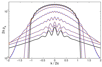
Figure 2: (Color online) Momentum distribution of the interacting Fermi gas. Dashed (orange) lines show results via the Bose Hubbard discretization, solid (blue) lines correspond to XXZ discretization. The interaction strength $g_{\text{F}}$ is $-51.2,-12.8,-3.2,-0.8,-0.2,-0.05$ from the broad to the narrow distributions. Solid (black) lines show the limiting cases of free fermions (narrow) and infinitely strong interacting fermions (broad, calculated from the formula given in Bender et al. (2005)). The calculations are done for $\Delta x=\frac{1}{64}$. Again there is perfect agreement between bosonic and fermionic discretization.

We now apply our method to the interacting Fermi gas in a harmonic trap,

$$H = -\frac{1}{2}\sum_{i=1}^{N}\partial_{x_{i}}^{2}$$ (24)

$$- \frac{g_{\text{F}}}{2}\sum_{j<i}\delta^{\prime}(x_{j}-x_{i})\left.\left(\partial_{x_{j}}-\partial_{x_{i}}\right)\right|_{x_{j}=x_{i^{+}}}$$

$$+ \sum_{i=1}^{N}\frac{1}{2}x_{i}^{2}.$$

We here chose the trap length to set the length scale. For $g_{\text{F}}=-\infty$ the system is called a fermionic Tonks-Girardeau gas Girardeau (1960); Girardeau and Minguzzi (2006); Minguzzi and Girardeau (2006). It can be treated analytically, since it maps to free bosons under the Bose Fermi mapping. E.g., the momentum distribution is known for arbitrary particle numbers Bender et al. (2005). It is of special experimental relevance, since it is equivalent to the density distribution measured in a time-of-flight experiment. However for intermediate interaction strength numerical calculations are required, which we are now able to do.

First we note, that we now have two options to discretized the model. Direct discretization will yield the XXZ Hamiltonian, while a Bose Fermi mapping will result in the Bose Hubbard Hamiltonian. Both methods of course have to produce exactly the same results.

Fig. 1 shows the spatial density distribution in the ground state for $N=25$ particles, i.e.,

$$\rho(x)=\int dx_{2}\dots dx_{N}\left|\phi(x,x_{2},\dots,x_{N})\right|,$$ (25)

which is approximated by the discretized system as the diagonal elements of $\langle a_{i}^{\dagger}a_{j}\rangle$. The ground state of the discretized system is calculated using a TEBD code and an imaginary time evolution, which has already been applied successfully to calculate the phase diagram of a disordered Bose Hubbard model Muth et al. (2008). The interaction strength is varied all the way from the free fermion regime to the regime of the fermionic Tonks-Girardeau gas. The density distribution changes accordingly from the profile of the free fermions, showing characteristic Friedel oscillations, to a narrow Gaussian peak for the fermionic Tonks-Girardeau gas. Note that the Bose Fermi mapping does not affect the local density, so the curves are the same for the corresponding bosonic system. I.e. the density distribution in the fermionic Tonks-Girardeau regime is identical to that of a condensate of non-interacting bosons. The curves obtained from the bosonic and fermionic lattice models are virtually indistinguishable which shows that both approaches are consistent.

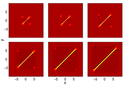
Figure 3: (Color online) single particle density matrix of the interacting Fermi gas calculated using XXZ discretization. Light regions are positive, dark regions negative. The interaction strength $g_{\text{F}}$ is $-51.2,-12.8$, and $-3.2$ (upper row) and $-0.8,-0.2$, and $-0.05$ (lower row). Remember that the cloud size is independent of the particle number towards the fermionic Tonks limit (because there is condensation in the bosonic picture) while it grow as $\sqrt{N}$ for free fermions.

The corresponding momentum distribution for the fermions,

$$\rho_{k}(k)=\int dk_{2}\dots dk_{N}\left|\phi(k,k_{2},\dots,k_{N})\right|,$$ (26)

which is quite different from that of the bosons, is shown in Fig. 2. It was obtained from the discretized wave function as the diagonal elements of the Fourier transform of $\langle a_{i}^{\dagger}a_{j}\rangle$. Again perfect agreement between the bosonic and fermionic lattice approximations can be seen. In accordance with physical intuition invoking the uncertainty relation and Pauli principle, the momentum distribution broadens as the real space distribution narrows. While for the free particles, real and momentum space description coincide for the harmonic oscillator the Friedel oscillations are deformed gradually towards the result for the fermionic Tonks-Girardeau gas calculated e.g. by Bender et al. Bender et al. (2005). The oscillations that remain in this limit are effects from the finite number of particles. They vanish as $1/N$ as can be seen from a Taylor expansion in $1/N$ of the expressions given in Bender et al. (2005) for the Fermi-Tonks case.

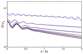
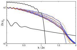
a) b) c)

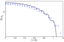
Figure 4: (Color online) momentum space distribution of the Fermi gas showing convergence of the method with discretization for a) the Fermi Tonks limit, b) $g_{\text{F}}=-0.8$, and c) the free fermionic case. Again in a) and b) dashed (orange) lines show results via the Bose Hubbard discretization, solid (blue) lines correspond to XXZ discretization. a) Results are shown for $\Delta x=\frac{1}{4},\frac{1}{8},\frac{1}{16},\frac{1}{32},\frac{1}{64},\frac{1}{128}$. As the grid gets finer, both discretization formulas converge to the exact result (black line). b) The same discretizations are used as in a) and we again observe convergence of both formulas towards a common limit, which is in this case not known analytically. The black lines are those showing up in a) and c) respectively and are for orientation. c) Note that in this case there is no sense in distinguishing the two formulas, since implementing $U=\infty$ always means excluding double occupation of sites by bosons which is immediately equivalent to simulating free fermions. We here only $\Delta x=\frac{1}{4}$ (circles), $\frac{1}{8}$ (crosses), $\frac{1}{128}$ (squares) to avoid confusion since the lines converge quite quickly. Although the squares sit perfectly on top of the exact result (black lines) they are not spaced densely enough to resolve the Friedel oscillations. This would require a lattice that extends across a region in space much larger than $N$ oscillator length where we have chosen to restrict the calculation to $20$ oscillator length to speed it up.

In Fig. 3 we have plotted the complete single particle density matrix

$$\rho(x,y)=\int dx_{2}\dots dx_{N}\phi^{*}(x,x_{2},\dots)\phi(y,x_{2},\dots)$$ (27)

for different interaction strength, starting from the Fermi-Tonks limit to the case of free fermions. One clearly recognizes two small off-diagonal peaks for larger interaction strength. The weight of these peaks, which are responsible for the oscillations in the momentum distribution, Fig. 2, to the remaining part near the diagonal is $\frac{1}{N}$, as can bee seen from analyzing the limiting case numerically, which can be done for much larger $N$ also. The sign of the peaks is positive only if $N$ is odd and negative for even $N$, so the momentum distributions in Fig. 2 would show a minimum at $k=0$ for all interaction strength if $N$ was chosen even instead of $25$.

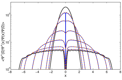
Figure 5: (Color online) density-density correlations of the interacting Fermi or Bose gas. The (orange) dashed lines show results obtained by Bose-Fermi mapping and solving the Bose Hubbard lattice model, the (blue) continuous lines correspond to the XXZ discretization. The interaction strength $g_{\text{F}}$ is $-51.2,-12.8,-3.2,-0.8,-0.2,-0.05$ from the narrow to the broad distributions. The solid black lines show the limiting cases of free fermions (broad) and infinitely strong interacting fermions (narrow, corresponds to free bosons). The calculations are done for $\Delta x=\frac{1}{64}$. One recognizes perfect agreement between the fermionic and bosonic discretization approaches apart from $x=0$ (see text). Note that both Fermions and Bosons with corresponding interaction show the same density-density correlations, since the quantity is invariant under the Bose-Fermi-mapping.

On first glance it may seem surprising that a mapping of a continuous, Bethe-Ansatz integrable Hamiltonian such as the Lieb-Liniger model to the non-integrable Bose-Hubbard model should produce accurate results. However, since the Lieb Liniger gas is dual to $p$-wave interacting fermions, as shown here its lattice approximation is equivalent to the spin 1/2 XXZ model, which is again Bethe-Ansatz integrable. Furthermore full recovery of the properties of the continuous model can of course only be expected in the limit $\Delta x\to 0$. In Fig.4 we have shown the momentum distribution of $p$-wave interacting fermions for decreasing discretization length $\Delta x$ for three different values of the interaction strength. One clearly recognizes convergence of the results as $\Delta x\to 0$. In the two analytically tractable cases of a free fermion gas and an the Fermi-Tonks gas the curves approach quickly the exact ones.

As a final application we calculate the real-space two-particle correlations in a trap. The corresponding results are shown in Fig. 5. Again the (blue) solid lines are obtained from the fermionic lattice model and the dashed (orange) lines from the dual bosonic model. Due to Pauli exclusion $g^{(2)}(0)=0$ and there is a pronounced dip in the $g^{(2)}$ near the origin for non interacting or weakly attractive fermions, while we see again Friedel oscillations for larger inter particle distances. In the dual bosonic case the dip is enforced by a strong repulsive interaction. As the fermionic attraction is increased, the depth of this dip is decreased. There is a smooth transition to the perfect Gaussian shape expected for the free bosons in the case of strongly interacting fermions.

Outside the point where the particle positions coincide both discretization formulas give the same result. There is a discontinuity maintaining $g^{(2)}(0)=0$ for the fermions, enforced by the symmetry of the wave functions. It should be noted that this singular jump is not reproduced in the dual bosonic model. This is because the duality mapping of the discretized models is only valid for two particles at different lattice sites and the dual bosonic model can only be used to calculate multi-particle correlations of fermions at pairwise different locations.

Finally we note that using the discretization formulas (12) and (18) one can of course also calculate other many body properties like off diagonal order Minguzzi and Girardeau (2006) using TEBD for larger systems. The method was also used to calculate out-of equilibrium dynamics for bosonic gases in the repulsive Muth et al. (2009) as well as attractive regime Muth and Fleischhauer (2010).

Special thanks go to Anna Minguzzi for stimulating discussions that have lead to this work. The authors would also like to thank Maxim Olshanii and Fabian Grusdt for valuable input. Finally the financial support of the graduate school of excellence MAINZ/MATCOR and the Sonderforschungsbereich TR49 are gratefully acknowledged.

References

- Kinoshita et al. (2004) T. Kinoshita, T. Wenger, and D. S. Weiss, Science 305, 1125 (2004).
- Paredes et al. (2004) B. Paredes, A. Widera, V. Murg, O. Mandel, S. Fölling, I. Cirac, G. V. Shlyapnikov, T. W. Hänsch, and I. Bloch, Nature 429, 277 (2004).
- Gunter et al. (2005) K. Gunter, T. Stoferle, H. Moritz, M. Kohl, and T. Esslinger, Physical Review Letters 95, 230401 (2005).
- Hofferberth et al. (2007) S. Hofferberth, I. Lesanovsky, B. Fischer, T. Schumm, and J. Schmiedmayer, Nature 449, 324 (2007).
- Haller et al. (2009) E. Haller, M. Gustavsson, M. J. Mark, J. G. Danzl, R. Hart, G. Pupillo, and H. C. Nägerl, Science 325, 1224 (2009).
- Bethe (1931) H. Bethe, Zeitschrift für Physik 71, 205 (1931).
- Lieb and Liniger (1963) E. H. Lieb and W. Liniger, Physical Review 130, 1605 (1963).
- Korepin et al. (1993) V. E. Korepin, N. M. Bogoliubov, and A. G. Izergin, Quantum Inverse Scattering Method and Correlation Functions (Cambridge University Press, 1993).
- Gaudin (1983) M. Gaudin, La Fonction d’Onde de Bethe (Paris: Masson, 1983).
- Giamarchi (2003) T. Giamarchi, Quantum Physics in One Dimension, vol. 121 of International Series of Monographs in Physics (Oxford Science Publications, 2003).
- White (1992) S. R. White, Physical Review Letters 69, 2863 (1992).
- Schollwöck (2005) U. Schollwöck, Reviews Of Modern Physics 77, 259 (2005).
- Vidal (2003) G. Vidal, Physical Review Letters 91, 147902 (2003).
- Vidal (2004) G. Vidal, Physical Review Letters 93, 040502 (2004).
- Girardeau (1960) M. Girardeau, Journal Of Mathematical Physics 1, 516 (1960).
- Cheon and Shigehara (1999) T. Cheon and T. Shigehara, Physical Review Letters 82, 2536 (1999).
- Schmidt and Fleischhauer (2007) B. Schmidt and M. Fleischhauer, Physical Review A 75, 021601(R) (2007).
- Schmidt et al. (2005) B. Schmidt, L. I. Plimak, and M. Fleischhauer, Physical Review A 71, 041601 (2005).
- Muth et al. (2009) D. Muth, B. Schmidt, and M. Fleischhauer, arXiv:0910.1749 (2009).
- Schmidt (2009) B. Schmidt, Ph.D. thesis, Technische Universität Kaiserslautern (2009).
- Cheon and Shigehara (1998) T. Cheon and T. Shigehara, Physics Letters A 243, 111 (1998).
- Girardeau and Olshanii (2004) M. D. Girardeau and M. Olshanii, Physical Review A 70, 023608 (2004).
- Seba (1986) P. Seba, Czechoslovak Journal of Physics 36, 667 (1986).
- Imambekov et al. (2009) A. Imambekov, A. A. Lukyanov, L. I. Glazman, and V. Gritsev, arXiv:0910.2269 (2009).
- Bender et al. (2005) S. A. Bender, K. D. Erker, and B. E. Granger, Physical Review Letters 95, 230404 (2005).
- Girardeau and Minguzzi (2006) M. D. Girardeau and A. Minguzzi, Physical Review Letters 96, 080404 (2006).
- Minguzzi and Girardeau (2006) A. Minguzzi and M. D. Girardeau, Physical Review A 73, 063614 (2006).
- Muth et al. (2008) D. Muth, A. Mering, and M. Fleischhauer, Physical Review A 77, 043618 (2008).
- Muth and Fleischhauer (2010) D. Muth and M. Fleischhauer, in preparation (2010).