Calculation of the spectrum of ¹²Li by using the multistep shell model method in the complex energy plane

Abstract

The unbound nucleus ¹²Li is evaluated by using the multistep shell model in the complex energy plane assuming that the spectrum is determined by the motion of three neutrons outside the ⁹Li core. It is found that the ground state of this system consists of an antibound $1/2^{+}$ state and that only this and a $1/2^{-}$ and a $5/2^{+}$ excited states are physically meaningful resonances.

I Introduction

The study of halo nuclei is one of the main subjects of research in nuclear physics at present. Many theoretical predictions on halo, superhalo and antihalo nuclei have been advanced in recent years hal1 ; hal2 ; hal3 . Most of these calculations correspond to nuclei very far from the stability line. They are mainly thought as a guide for experiments to be performed in coming facilities. The general feature found in these calculations is that a necessary condition for a nucleus to develop a halo is that the outmost nucleons move in shells which extend far in space. That is, only a weak barrier keep the system within the nuclear volume. These shells may be resonances, antibound states (also called virtual states), or even low-spin bound states which lie very close to the continuum threshold. These conditions are fulfilled by the nucleus ¹¹Li and also heavier Li isotopes. There are a number of experiments which have been performed in these very unstable isotopes in order to get information about the structure of halos bau07 . In particular we will concentrate our attention to Refs. aks08 ; pat10 ; hal10 where the spectrum of ¹²Li was measured. Our aim is to analyze these experimental data by using a suitable formalism to treat unstable nuclei. This formalism is an extension of the shell model to the complex energy plane and is therefore called complex shell model idb02 , although the name Gamow shell model is also used mic02 . In addition, the correlations induced by the pairing force acting upon particles moving in decaying single-particle states will be taken into account by using the multistep shell model (MSM) blo84 .

The formalism is presented in Section II. Applications are in Section III and a summary and conclusions are in Section IV.

II The formalism

The study of unstable nuclei is a very difficult undertaking since, in principle, time dependent formalisms should be used to describe the motion of a decaying nucleus. However, the system may be considered stationary if it lives a long time. In this case the time dependence can be circumvented. In fact, often unstable nuclei live a very long time and therefore they may be considered bound as, e.g., in alpha decaying states of many heavy isotopes, like ²⁰⁸Bi or ¹⁸⁰Ta(9^-), with $T_{1/2}>10^{15}y$. On the other hand, experimental facilities allow one nowadays to measure systems living a very short time. To describe these short time processes one has to consider the decaying character of the system. This is shown, e.g., by the failure of the shell model calculation of Ref. pop85 , performed by using a standard bound representation, to explain even the ground state of ¹²Li aks08 .

Of the various theories that have been conceived to analyze unbound systems, we will apply an extension of the shell model to the complex energy plane idb02 . The basic assumption of this theory is that resonances can be described in terms of states lying in the complex energy plane. The real parts of the corresponding energies are the positions of the resonances while the imaginary parts are minus twice the corresponding widths, as it was proposed by Gamow at the beginning of quantum mechanics gam28 . These complex states correspond to solutions of the Schrödinger equation with outgoing boundary conditions. We will not present here the formalism in detail, since this was done many times before, e.g., in Refs. cxsm ; mic09 . Rather, we will give the main points necessary for the presentation of the applications.

II.1 The Berggren representation

In this Subsection we will very briefly describe the representation to be used here.

The eigenstates of a central potential obtained as outgoing solutions of the Schrödinger equation can be used to express the Dirac $\delta$-function as b68

$$\delta(r-r^{\prime})=\sum_{n}w_{n}(r)w_{n}(r^{\prime})+\int_{L^{+}}dEu(r,E)u(r^{\prime},E),$$ (1)

where the sum runs over all the bound and antibound states plus the complex states (resonances) which lie between the real energy axis and the integration contour $L^{+}$. The wave function of a state $n$ in these discrete set is $w_{n}(r)$ and $u(r,E)$ is the scattering function at energy $E$. The antibound states are virtual states with negative scattering length. They are fundamental to describe nuclei in the Li region thz .

Discretizing the integral of Eq. (1) one obtains the set of orthonormal vectors $|\varphi_{j}\rangle$ forming the Berggren representation lio96 . Since this discretization provides an approximate value of the integral, the Berggren vectors fulfill the relation $I\approx\sum_{j}|\varphi_{j}\rangle\langle\varphi_{j}|$, where all states, that is bound, antibound, resonances and discretized scattering states, are included. The corresponding single-particle wave functions are

$$\langle\vec{r}|\varphi_{i}\rangle=R_{n_{i}l_{i}j_{i}}(r)\big{(}\chi_{1/2}Y_{l_{i}}({\hat{r}})\big{)}_{j_{i}m_{i}},$$ (2)

where $\chi$ is the spin wave function and

$$R_{n_{i}l_{i}j_{i}}(r)=\phi_{n_{i}l_{i}j_{i}}(r)/r$$ (3)

is the radial wave function fulfilling the Berggren metric, according to which the scalar product between two functions consists of one function times the other (for details see Ref. lio96 ), i.e.,

$$\int_{0}^{\infty}dr\phi_{n_{i}l_{i}j_{i}}(r)\phi_{n^{\prime}_{i}l_{i}j_{i}}(r)=\delta_{n_{i}n_{i}^{\prime}}.$$ (4)

Using the Berggren representation one readily gets the two-particle shell-model equations in the complex energy plane (CXSM) cxsm , i.e.,

$$(W(\alpha_{2})-\epsilon_{i}-\epsilon_{j})X(ij;\alpha_{2})=\sum_{k\leq l}\langle\tilde{k}\tilde{l};\alpha_{2}|V|ij;\alpha_{2}\rangle X(kl;\alpha_{2}),$$ (5)

where $V$ is the residual interaction. The tilde in the interaction matrix element denotes mirror states so that in the corresponding radial integral there is not any complex conjugate, as required by the Berggren metric. The two-particle states are labeled by $\alpha_{2}$ and Latin letters label single-particle states. $W(\alpha_{2})$ is the correlated two-particle energy and $\epsilon_{i}$ is single-particle energy. The two-particle wave function is given by

$$|\alpha_{2}\rangle=P^{+}(\alpha_{2})|0\rangle,$$ (6)

where the two-particle creation operator is given by

$$P^{+}(\alpha_{2})=\sum_{i\leq j}X(ij;\alpha_{2})\frac{(c^{+}_{i}c^{+}_{j})_{\lambda_{\alpha_{2}}}}{\sqrt{1+\delta_{ij}}},$$ (7)

and $\lambda_{\alpha_{2}}$ is the angular momentum of the two-particle state.

We will use a separable interaction as in Ref. ant , which describes well the states of ¹¹Li. The energies are thus obtained by solving the corresponding dispersion relation. The two-particle wave function amplitudes are given by

$$X(ij;\alpha_{2})=N_{\alpha_{2}}\frac{f(ij,\alpha_{2})}{\omega_{\alpha_{2}}-(\epsilon_{i}+\epsilon_{j})},$$ (8)

where $f(ij,\alpha_{2})$ is the single particle matrix element of the field defining the separable interaction and $N_{\alpha_{2}}$ is the normalization constant determined by the condition $\sum_{i\leq j}X(ij;{\alpha_{2}})^{2}=1$.

The spectrum of ¹¹Li was already evaluated within the CXSM including antibound states ant . Here we will repeat that calculation in order to determine the two-particle states to be used in the calculation of the three-particle system, i.e., ¹²Li. For this we will use the Multistep Shell Model Method, which we will briefly describe below.

II.2 The Multistep Shell Model Method

As its name indicates, the Multistep Shell Model Method (MSM) solves the shell model equations in several steps. In the first step the single-particle representation is chosen. In the second step the energies and wave functions of the two-particle system are evaluated by using a given two-particle interaction. The three-particle states are evaluated in terms of a basis consisting of the tensorial product of the one- and two-particle states previously obtained. In this and subsequent steps the interaction does not appear explicitly in the formalism. Instead, it is the wave functions and energies of the components of the MSM basis that replace the interaction. The MSM basis is overcomplete and non-orthogonal. To correct this one needs to evaluate the overlap matrix among the basis states also. A general description of the formalism is in Ref. lio82 . The particular system that is of our interest here, i.e., the three-particle case, can be found in Ref. blo84 , where the MSM was applied to study the three-neutron hole states in the nucleus ²⁰⁵Pb.

Using the Berggren single-particle representation described above, we will evaluate the complex energies and wave functions of ¹²Li using the MSM basis states consisting of the Berggren one-particular states, which are states in ¹⁰Li, times the two-particle states corresponding to ¹¹Li. Below we refer to this formalism as CXMSM.

The three-particle energies $W(\alpha_{3})$ are given by blo84

$$(W(\alpha_{3})-\varepsilon_{i}-W(\alpha_{2}))\langle\alpha_{3}|(c^{+}_{i}P^{+}(\alpha_{2}))_{\alpha_{3}}|0\rangle\\ =\sum_{j\beta_{2}}\left\{\sum_{k}(W(\beta_{2})-\varepsilon_{i}-\varepsilon_{k})A(i\alpha_{2},j\beta_{2};k)\right\}\\ \times\langle\alpha_{3}|(c^{+}_{j}P^{+}(\beta_{2}))_{\alpha_{3}}|0\rangle,$$ (9)

where

$$A(i\alpha_{2},j\beta_{2};k)=\hat{\alpha}_{2}\hat{\beta}_{2}\left\{\begin{array}[]{ccc}i&k&\beta_{2}\\ j&\alpha_{3}&\alpha_{2}\end{array}\right\}Y(kj;\alpha_{2})Y(ki;\beta_{2}),\\$$ (10)

$$Y(ij;\alpha_{2})=(1+\delta(i,j))^{1/2}X(ij;\alpha_{2}),$$ (11)

and the rest of the notation is standard.

The matrix defined in Eq. (9) is not hermitian and the dimension may be larger than the corresponding shell-model dimension. This is due to the violations of the Pauli principle as well as overcounting of states in the CXMSM basis. Therefore the direct diagonalization of Eq. (9) is not convenient. One needs to calculate the overlap matrix in order to transform the CXMSM basis into an orthonormal set. In this three-particle case the overlap matrix is

$$\left\langle 0|(c^{+}_{i}P^{+}(\alpha_{2}))^{{\dagger}}_{\alpha_{3}}(c^{+}_{j}P^{+}(\beta_{2}))_{\alpha_{3}}|0\right\rangle\\ =\delta_{ij}\delta_{\alpha_{2}\beta_{2}}+\sum_{k}A(i\alpha_{2},j\beta_{2};k).$$ (12)

Using this matrix (12) one can transform the matrix determined by Eq. (9) into a hermitian matrix $T$ which has the right dimension. The diagonalization of $T$ provides the three-particle energies. The corresponding wave function amplitudes can be readily evaluated to obtain

$$|\alpha_{3}\rangle = P^{+}(\alpha_{3})|0\rangle,$$ (13)

$$P^{+}(\alpha_{3}) = \sum_{i\alpha_{2}}X(i\alpha_{2};\alpha_{3})(c^{+}_{i}P^{+}(\alpha_{2}))_{\alpha_{3}},$$ (14)

where $P^{+}(\alpha_{3})$ is the three-particle creation operator.

It has to be pointed out that in cases where the basis is overcomplete the amplitudes $X$ are not well defined. But this is no hinder to evaluate the physical quantities. For details see Ref. blo84 .

The advantage of the MSM in stable nuclei is that one can study the influence of collective vibrations upon nuclear spectra within the framework of the shell model. Thus, in Ref. blo84 the multiple structure of particle-vibration coupled states in odd Pb isotopes was analyzed.

But the most important feature for our purpose is that the CXMSM allows one to choose in the basis states a limited number of excitations. This is because in the continuum the vast majority of basis states consists of scattering functions. These do not affect greatly physically meaningful two-particle states. That is, the majority of the two-particle states provided by the CXSM are complex states which form a part of the continuum background. Only a few of those calculated states correspond to physically meaningful resonances, i.e., resonances which can be observed. Below we call a “resonance” only to a complex state which is meaningful. These resonances are mainly built upon single-particle states which are either bound or narrow resonances. Yet, one cannot ignore the continuum when evaluating the resonances. The continuum configurations in the resonance wave function are small but many, and they affect the two-particle resonance significantly cxsm . That is, the important continuum configurations to induce resonances are contained in the corresponding resonance wave functions. Therefore, the great advantage of the CXMSM is that one can include in the basis only two-particle resonances, while neglecting the background continuum states, which form the vast majority of complex two-particle states. The question is which are the two-particle states that are indeed resonances. This, and also the question of how to evaluate and recognize the physically meaningful three-particle states, are addressed in the next Section.

III Applications

In this Section we will apply the CXMSM formalism described above to study the nucleus ¹²Li. As in Ref. ant , we will take the core to be the nucleus ⁹Li. This is justified since the three protons included in this core can be considered frozen and, therefore, merely spectators ber91 .

To evaluate the valence shells we will proceed as in Refs. esb97 ; pac02 ; idb04 and choose as central field a Woods-Saxon potential with different depths for even and odd orbital angular momenta $l$. The corresponding parameters are (in parenthesis for odd $l$-values) $a$= 0.670 fm, $r_{0}$ = 1.27 fm, $V_{0}$ = 50.0 (36.9) MeV and $V_{\rm so}$=16.5 (12.6) MeV. As in Ref. idb04 , we thus found the single-particle bound states $0s_{1/2}$ at -23.280 MeV and $0p_{3/2}$ at -2.589 MeV forming the ⁹Li core. The valence shells are the low lying resonances $0p_{1/2}$ at (0.195,-0.047) MeV and $0d_{5/2}$ at (2.731, -0.545) MeV and the shell $0d_{3/2}$ at (6.458,-5.003) MeV. This cannot be considered as a resonance, since it is so wide that rather it is a part of the background. Besides, the state $1s_{1/2}$ appears as an antibound state at -0.050 MeV. We thus reproduce the experimental single-particle energies as given in Ref. boh97 . We also found other states at higher energies, but they do not affect our calculation because they are very high and also very wide to be considered as meaningful resonances. We thus include in our Berggren representation only the antibound state $1s_{1/2}$ and the resonances $0p_{1/2}$ and $0d_{5/2}$.

The energy of the resonance $0p_{1/2}$ has been contested and instead the value (0.563,-0.252) MeV was proposed aks08 . Since this is an important quantity in the determination of the two- and three-particle spectra, we will use both of them in our calculations. We obtained this $0p_{1/2}$ energy (i.e., (0.563,-0.252) MeV) by choosing $V_{0}$=34.755 MeV for $l$ odd while keeping all the other parameters as before.

To define the Berggren single-particle representation we still have to choose the integration contour ${L^{+}}$ (see Eq. (1)).

To include in the representation the antibound $1s_{1/2}$ state as well as the Gamow resonances $0p_{1/2}$ and $0d_{5/2}$ we will use two different contours. The number of points on each contour defines the energies of the scattering functions in the Berggren representation, i.e., the number of basis states corresponding to the continuum background. This number is not uniformity distributed, since in segments of the contour which are close to the antibound state or to a resonance the scattering functions increase strongly. We therefore chose the density of points to be larger in those segments.

We include the antibound state by using the contour in Fig. 1.

Figure 1: Contour used to include the antibound state (see, also, Ref. idb04 ). The points $B_{i}$ denote bound state energies while $A$ denotes the antiboud state. The points $V_{i}$ correspond to the vertices defining the contour. They have the values $V_{1}$=(-0.05,0.05) MeV, $V_{2}$=(-0.1,0) MeV, $V_{3}$=(0,-0.4) MeV, $V_{4}$=(0.5,-0.4) MeV, $V_{5}$=(8,-0.4) MeV, $V_{6}$=(8,0) MeV and $V_{7}$=(10,0) MeV

The number of points in each segment are given in Table 1.

Table 1: Number of Gaussian points in the different segments of the contour of Fig. 1.

Segment	[$(0,0)-V_{1}$]	[$V_{1}-V_{2}$]	[$V_{2}-V_{3}$]	[$V_{3}-V_{4}$]	[$V_{4}-V_{5}$]	[$V_{5}-V_{6}$]	[$V_{6}-V_{7}$]
Number	30	30	30	30	30	16	6

Figure 2: Contour used to include the Gamow resonances represented by the points $G_{i}$. The vertices are $V_{1}$=(0,-1) MeV, $V_{2}$=(1,-1) MeV, $V_{3}$=(8,-1) MeV, $V_{4}$=(8,0) MeV and $V_{5}$=(10,0) MeV.

For the Gamow resonances the contour in Fig. 2 is used with the number of Gaussian points as in Table 2.

Table 2: Number of Gaussian points in the different segments of the contour of Fig. 2.

Segment	[$(0,0)-V_{1}$]	[$V_{1}-V_{2}$]	[$V_{2}-V_{3}$]	[$V_{3}-V_{4}$]	[$V_{4}-V_{5}$]
Number	30	30	30	8	4

We have adopted these points after verifying that the results converged to their final values. A discussion about the choice of these contours and also on the physical meaning of the antibound state can be found in Ref. ant .

With the single-particle representation thus defined we proceed to evaluate the two-particle states.

III.1 Two-particle states: the nucleus ¹¹Li.

The only state which is measured in ¹¹Li is its bound ground state, which was found to lie at an energy of -0.295 MeV gar . However, this state is more bound than that, as it was determined in more recent experiments smi08 ; bac08 ; rog09 . We will adopt the most precise of these values, i.e., -0.369 MeV smi08 . The corresponding angular momentum is $3/2^{-}$. This spin arises from the odd proton lying deep in the spectrum coupled to two neutrons. As has been already mentioned, the proton is considered to be a spectator. The dynamics of the system is thus determined by the pairing force acting upon the two neutrons coupled to a state $0^{+}$, which behaves as a normal even-even ground state esb97 ; ant . Besides the energy, this state has been measured to have an angular momentum contain of about 60 % of s-waves and 40 % of p-waves, although small components of other angular momenta are not excluded gar .

We will perform the calculation of the two-particle states by using the separable interaction discussed in Section II. The strength $G_{\lambda_{2}}$, corresponding to the states with angular momentum $\lambda_{2}$ and parity $(-1)^{\lambda_{2}}$, will be determined by fitting the experimental energy of the lowest of these states, as usual. It is worthwhile to point out that $G_{\lambda_{2}}$ defines the Hamiltonian and, therefore, is a real quantity. The two-particle energies are found by solving the corresponding dispersion relation while the two-particle wave function components are as in Eq. (8).

Table 3: Angular momentum contain of ¹¹Li(gs) corresponding to the energies $\epsilon_{p_{1/2}}$ discussed in the text.

	component(%)
$\epsilon_{p_{1/2}}$ (MeV)	s-waves	p-waves	d-waves
(0.195,-0.047)	46.8	49.1	4.2
(0.563,-0.252)	72.6	20.9	6.4

The angular momentum contains of the ground state wave function are shown in Table 3. One sees that for the case in which the single-particle state $0p_{1/2}$ is assumed to lie at (0.195,-0.047) MeV the two-particle wave function consists of 46.8% $s$-states and 49.1% $p$-states which are reasonable values. For the $0p_{1/2}$ energy at (0.563,-0.252) MeV the angular momentum contain is 72.6 % $s$-states and 20.9 % $p$-states, which is also acceptable, specially considering that it provides the correct order of the relative magnitudes. Both cases are in reasonable agreement with experiment.

The wave function components corresponding to this state are strongly dependent upon the contour that one uses. However, measurable quantities, like the energies and transition probabilities, do not. This is because the physical quantities are defined on the real energy axis and, therefore, they remain the same when changing contour. But complex states which are part of the continuum background do not have any counterpart on the real energy axis and the physical quantities for these states acquire different values for different contours ant . We will use this property to determine whether a complex state is a meaningful resonance. This is important, since the ground state is the only one for which experimental data exists. There might be other meaningful states that have not been found yet. This implies that we have to evaluate all possible two-particle states which are spanned by our single-particle representation. To decide whether a state thus calculated is a meaningful resonance we will proceed as in Refs. ant ; gpr and analyze the singlet ($S=0$) component of the two-particle wave function. The corresponding expression for this component was given in Eq. (10) of Ref. gpr , but we will show it here again for clarity of presentation. For the state $\alpha$ with spin and spin-projection $(JM)$ that component is, with standard notation,

$$\Psi_{\alpha JM}(\vec{r}_{1}\vec{r}_{2})=\left[\chi_{1/2}(1)\chi_{1/2}(2)\right]_{0}^{0}\sum_{a\leq b}X(ab,\alpha JM)\hat{j}_{a}\hat{j}_{b}\\ \times\left[C(ab,\vec{r}_{1}\vec{r}_{2})-(-)^{j_{a}+j_{b}-J}C(ba,\vec{r}_{1}\vec{r}_{2})\right]$$ (15)

where

$$C(ab,\vec{r}_{1}\vec{r}_{2})=\phi_{a}(r_{1})\phi_{b}(r_{2})(-)^{l_{b}+1/2-j_{a}+J}\\ \times\left\{\begin{array}[]{ccc}l_{a}&j_{a}&1/2\\ j_{b}&l_{b}&J\\ \end{array}\right\}\left[Y_{l_{a}}(\hat{r}_{1})Y_{l_{b}}(\hat{r}_{2})\right]_{J}^{M},$$ (16)

and $\phi_{a}(r)$ is the radial wave function corresponding to the single-particle state $a$ (Eq. (3)).

If the two-particle state $(\alpha JM)$ is a meaningful resonance then the wave function above should be localized within a region extending not too far outside the nuclear surface, and its imaginary part should not be too large ant . To study these features it is not necessary to go to all six dimensions corresponding to the coordinates $\vec{r}_{1}$ and $\vec{r}_{2}$. In fact it is enough to consider the coordinate $r$ given by $\vec{r}_{1}=\vec{r}_{2}=\vec{r}=(0,0,r)$ which corresponds to the two particles located at the same point and in the z-direction. For details see gpr . We will call this one-dimensional function $\Psi_{\alpha JM}(r)$.

The evaluation of the $0^{+}$ states is a relatively easy task, since in this case we have determined the strength $G_{0^{+}}$ by fitting the experimental energy of ¹¹Li(gs). With this value of the strength we calculated all the $0^{+}$ states and found that there is no any meaningful resonance. The only physically meaningful $0^{+}$ state is the bound ground state. Besides this, we found that there is a meaningful resonance, which is the state $2^{+}_{1}$ at an energy (2.300,-0.372) MeV. In Fig. 6 we show the corresponding radial wave function $\Psi_{2^{+}_{1}}(r)$. One sees that it is rather localized and that its imaginary part is relatively small as compared to the corresponding real part. This is a state which perhaps is at the limit of what can be considered a meaningful resonance. Yet, it is not too wide and it has an effect on the physical three-particle states, as will be seen below. It is worthwhile to point out that the width of this state (744 keV) is the escape width. At high energies, where the giant resonances lie, most of the width consists of the spreading width, i.e., of mixing with particle-hole configurations gal88 . However, at the low energies of the states that we study this mixing would not be relevant.

We have thus found that the only two-particle states on which physically meaningful three-particle states can be built are ¹¹Li(gs) and ¹¹Li($2^{+}_{1}$). One can understand why there are so few meaningful two-particle states in this nucleus by looking at the radial wave functions of the single-particle states that form the representation. For the antibound state one sees in Fig. 3 that it extends in an increasing rate far out from the nuclear surface, as expected in this halo nucleus (the standard value of the radius is here $1.2\times 11^{1/3}$=2.7 fm). The radial wave function corresponding to the Gamow resonance $0p_{1/2}$ is shown in Fig. 4. The state ¹¹Li($2^{+}_{1}$) is determined by the antibound state and the $0d_{5/2}$ resonance, which has a large and increasing imaginary part at relative short distances, as shown in Fig. 6. These single-particle wave functions have large imaginary parts and a divergent nature even at rather short distances from the nucleus. In other words, they correspond to states that live a time which is too short to produce meaningful two-particle resonances.

An important point for the analysis of the three-particle states to be performed below, is that the scattering wave functions in the segments $[(0,0)-V_{1}]$, $[V_{1}-V_{2}]$ and $[V_{2}-V_{3}]$ are similar in magnitude to the wave function of the antibound state. This is because the segments are very close to the antibound state ant . This is a feature that cannot be avoided, and is due to the attractive character of the pairing force. That is, the lowest single-particle configuration in the Berggren basis is $V_{2}^{2}$, with energy $-2\epsilon$, where $V_{2}=(-\epsilon,0)$. This configuration has to lie above the energy of the two-particle correlated state, i. e. it has to be $\epsilon>\omega(^{11}$Li(gs))/2.

Figure 3: Radial function $\phi(r)$ corresponding to the single-particle neutron anti bound state $0s_{1/2}$ at an energy of -0.050 MeV.

Figure 4: As Fig. 3 but for the Gamow resonance $0p_{1/2}$ at an energy of (0.563,-0.252) MeV. The dashed line is the imaginary part of the wave function.

Figure 5: As Fig. 3 but for the Gamow resonance $0d_{5/2}$ at an energy of (2.731,-0.545) MeV. The dashed line is the imaginary part of the wave function.

Figure 6: Radial function $\Psi(r)$ corresponding to the two-particle state ¹¹Li($2^{+}_{1}$) at an energy of (2.300,-0.372)MeV. The dashed line is the imaginary part of the wave function.

With the states $0^{+}_{1}$ and $2^{+}_{1}$ thus calculated we proceeded to the calculation of the three-particle system within the CXMSM.

III.2 Three-particle states: the nucleus ¹²Li.

With the single-particle states and the two-particle states ¹¹Li(gs) and ¹¹Li($2^{+}_{1}$) discussed above, we formed all the possible three-particle basis states. We found that the only physically relevant states are those which are mainly determined by the bound state ¹¹Li($0^{+}_{1}$). The corresponding spins and parities are $1/2^{+}$, $1/2^{-}$ and $5/2^{+}$. States like $3/2^{+}$, which arises from the CXMSM configuration $|1s_{1/2}\otimes 2^{+}_{1};3/2^{+}>$, is not a meaningful state.

Due to the large number of scattering states included in the single-particle representation the dimension of three-particle basis is also large. The scattering states are needed in order to describe these unstable states.

In the calculations we took into account all the possibilities described above regarding the energies of the single-particle state $0p_{1/2}$ as well as the binding energy of the state ¹¹Li(gs). The corresponding results are shown in Tables 4 and 5. Comparing these two Tables one sees that the state $1/2^{+}$ depends very slightly on the energy $\epsilon_{p_{1/2}}$ but rather strongly on ${\omega_{\alpha_{2}}}$. Instead. this tendency is opposite for the states $1/2^{-}$ and $5/2^{+}$.

Table 4: Calculated three-particle states in ¹²Li (in MeV) corresponding to the two energies $\epsilon_{p_{1/2}}$ of Table 3 and the two-particle energies taken to be ${\omega_{0^{+}_{1}}}=-0.295$MeV and ${\omega_{2^{+}_{1}}}=(2.300,-0.372)$MeV.

$\epsilon_{p_{1/2}}$	$1/2^{+}$	$1/2^{-}$	$5/2^{+}$
(0.195,-0.047)	(-0.386,-0.006)	(0.821,-0.189)	(1.348,-0.276)
(0.563,-0.252)	(-0.382,-0.006)	(1.114,-0.403)	(1.169,-0.242)

The most important feature in these Tables is that the lowest state is $1/2^{+}$ and that it has a real and negative energy. It is an antibound state, as it is the $1s_{1/2}$ state itself. A manifestation of this is that the radial wave function diverges at large distances.

Accepting the latest reported values for the energies of the states $0p_{1/2}$ and ¹¹Li(gs), i.e., those in the second line of Table 5, our calculation predicts, besides the antibound $1/2^{+}$ state, a state $1/2^{-}$ at (1.116,-0.411) MeV and a state $5/2^{+}$ at (1.148,-0.243) MeV. This assignment agrees well with what is given in Ref. aks08 for the ground state of ¹²Li, which was found to be an antibound (or virtual) state. In the same fashion, in Ref. pat10 a state was found at 1.5 MeV which probably has spin and parity $5/2^{+}$. In these experiments the angular momentum contain of the states were measured and therefore it is proper to compare the experimental quantities with our calculations, where only neutrons are considered.

Table 5: As Table 4 but for ${\omega_{0^{+}}}=-0.369$MeV.

$\epsilon_{p_{1/2}}$	$1/2^{+}$	$1/2^{-}$	$5/2^{+}$
(0.195,-0.047)	(-0.466,-0.011)	(0.753,-0.206)	(1.315,-0.276)
(0.563,-0.252)	(-0.466,-0.011)	(1.116,-0.411)	(1.148,-0.243)

In Ref. hal10 it was also found that ¹²Li(gs) is an antibound state but, in addition, two other low-lying states were observed at 0.250 MeV and 0.555 MeV by using two-proton removal reactions. In this case the $0p_{3/2}$ proton in the core may interfere with the neutron excitations evaluated above. In particular, the antibound $1/2^{+}$ ground state would provide, through the proton excitation, a state $1^{-}$ and a $2^{-}$. This is the situation encountered in the shell model calculation presented in Ref. hal10 . As we have pointed out above, from the CXMSM viewpoint the very unstable states determining the spectrum in this nucleus, with wave functions which are both diverging and complex, can hardly be described by harmonic oscillator representations. To investigate the relation between the results provided by both representations we repeated the shell-model calculation of Ref. hal10 . We thus took ⁴He as the core and used the WBT effective interaction war92 ; bro01 . The resulting Hamiltonian matrix was diagonalized by using the code described in qi08 . The corresponding calculated energies, which agree with those presented in hal10 , are shown in Fig. 7.

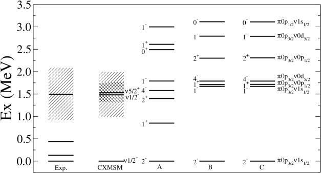
Figure 7: Experimental level scheme in ¹²Li. The three lowest levels are from hal10 , while the one at 1.5 MeV is from pat10 . In the second column are the three-neutron CXMSM results. In the columns A-C are the shell-model calculations corresponding to different truncation schemes: A) within $0-1\hbar\omega$ excitations, B) within $0-3\hbar\omega$ excitations and C) full $psd$ space. Dashed lines indicate the widths of the resonances.

One sees in this Figure that the full calculation predicts all excited states to lie well above the corresponding experimental values. It is worthwhile to point out that the calculated states exhibit rather pure shell model configurations. For instance the states $2^{-}_{1}$ (ground state) and $1^{-}_{1}$ are mainly composed of the configuration $|\pi\left[0p_{3/2}\right]\nu\left[(0p_{1/2})^{2}1s_{1/2}\right]\rangle$. This does not fully agree with our CXMSM calculation, since in our case this wave function is mainly of the form $|1s_{1/2}\otimes^{11}{\rm Li(gs)}\rangle$. This differs from the shell model case in two ways. First, the state ¹¹Li(gs) contains nearly as much of $1s_{1/2}$ as of $0p_{1/2}$. Second the continuum states contribute much in the building up of the antibound ¹²Li(gs) wave function, as discussed above. In our representation it is straightforward to discern the antibound character of this state, which is not the case when using harmonic oscillator bases.

The shell model splittings between states originated from the same configurations in Fig. 7 are due to the neutron-proton interaction, which in some cases can be large. For instance, the matrix elements $\langle\pi[0p_{3/2}]\nu[0p_{1/2}];J|V|\pi[0p_{3/2}]\nu[0p_{1/2}];J\rangle$ are strong and attractive tal60 .

Given all the uncertainties related to these calculations in the continuum, and the scarce amount of experimental data, we will not attempt to evaluate the ¹²Li states by adding a new uncertainty which would be the inclusion of a proton-neutron interaction.

Considering the limitations that one expects from a calculation of very unstable states by using harmonic oscillator basis, the rather good agreement between the shell-model and the CXMSM presented above is surprising. In contrast to the shell-model, the CXMSM provides not only the energies but also the widths of the resonances. It is therefore very important to encourage experimental groups to try to obtain these quantities in order to probe the formalisms.

IV Summary and conclusions

In this paper we have studied excitations occurring in the continuum part of the nuclear spectrum which are at the limit of what can be observed within present experimental facilities. These states are very unstable but yet live a time long enough to be amenable to be treated within stationary formalisms. We have thus adopted the CXSM (shell model in the complex energy plane cxsm ) for this purpose. In addition we performed the shell model calculation by using the multistep shell model. In this method of solving the shell model equations one proceeds in several steps. In each step one constructs building blocks to be used in future steps lio82 . We applied this formalism to analyze ¹²Li as determined by the neutron degrees of freedom, i.e., the three protons in the core were considered to be frozen. In this case the excitations correspond to the motion of three particles, partitioned as the one-particle times the two-particle systems. This formalism was applied before, e.g., to study multiplets in the lead region blo84 .

By using single-particle energies (i.e., states in ¹⁰Li) as provided by experimental data when available or as provided by our calculation, we found that the only physically meaningful two-particle states are ¹¹Li(gs), which is a bound state, and ¹¹Li($2^{+}_{1}$), which is a resonance. As a result there are only three physically meaningful states in ¹²Li which, besides the antibound ground state, it is predicted that there is a resonance $1/2^{-}$ lying at about 1 MeV and about 800 keV wide and another resonance which is $5/2^{+}$ lying at about 1.1 MeV and 500 keV wide. That the ground state is an antibound (or virtual) state was confirmed by a number of experiments aks08 ; pat10 ; hal10 and the state $5/2^{+}$ has probably been observed in pat10 . However, in hal10 two additional states, lying at rather low energies, have been observed which do not seem to correspond to the calculated levels. It has to be mentioned that neither a shell model calculation, performed within an harmonic oscillator basis, provides satisfactory results in this case. Yet, we found that this shell model calculation works better than one would assume given the unstable character of the states involved. We therefore conclude that in order to probe the formalisms that have been introduced to describe these very unstable systems additional experimental data, specially regarding the widths of the resonances, would be required.

References

- (1) V. Rotival, K. Bennaceur, and T. Duguet, Phys. Rev. C 79, 054309 (2009).
- (2) N. Schunck and J.L. Egido, Phys. Rev. C 78, 064305 (2008).
- (3) M. Grasso, S. Yoshida, N. Sandulescu, and N. Van Giai, Phys. Rev. C 74, 064317 (2006).
- (4) T. Baumann et al., Nature 449, 1022 (2007).
- (5) Yu. Aksyutina et al., Phys. Lett. B666, 430 (2008).
- (6) T. Roger, PhD thesis; P. Roussel Chomaz et al., to be published.
- (7) C. C. Hall et al., Phys. Rev. C 81, 021302(R) (2010).
- (8) R. Id Betan, R. J. Liotta, N. Sandulescu, and T. Vertse, Phys. Rev. Lett. 89, 042501 (2002).
- (9) N. Michel, W. Nazarewicz, M. Ploszajczak, and K. Bennaceur, Phys. Rev. Lett. 89, 042502 (2002).
- (10) J. Blomqvist, R. J. Liotta, L. Rydstrom, and C. Pomar, Nucl. Phys. A423, 253 (1984).
- (11) N. A. F. M. Poppelier, L. D. Wood, and P. W. M. Glaudemans, Phys. Lett. B157, 120 (1985).
- (12) G. Gamow, Z. Phys. 51, 204 (1928).
- (13) R. Id Betan, R. J. Liotta, N. Sandulescu, and T. Vertse, Phys. Rev. C 67, 014322 (2003).
- (14) N. Michel, W. Nazarewicz, M. Płoszajczak, and T. Vertse, J. Phys. G36, 013101 (2009).
- (15) T. Berggren, Nucl. Phys. A109, 265 (1968).
- (16) I. J. Thompson and M. V. Zhukov, Phys. Rev. C 49, 1904 (1994).
- (17) R. J. Liotta, E. Maglione, N. Sandulescu, and T. Vertse, Phys. Lett. B367, 1 (1996).
- (18) R. Id Betan, R. J. Liotta, N. Sandulescu, T. Vertse, and R. Wyss, Phys. Rev. C 72, 054322 (2005).
- (19) R. J. Liotta and C. Pomar, Nucl. Phys. A382, 1 (1982).
- (20) G. F. Bertsch and H. Esbensen, Ann. Phys. (New York) 209, 327 (1991).
- (21) H. Esbensen, G.F. Bertsch, and K. Hencken, Phys. Rev. C 56, 3054 (1997), and references therein.
- (22) J.C. Pacheco and N. Vinh Mau, Phys. Rev. C 65, 044004 (2002).
- (23) R. Id Betan, R.J. Liotta, N. Sandulescu, and T. Vertse, Phys. Lett. B584, 48 (2004).
- (24) H.G. Bohlen, et al., Nucl. Phys. A616, 254c (1997).
- (25) E. Garrido, D. V. Fedorov, and A. S. Jensen, Nucl. Phys. A700, 117 (2002).
- (26) C. Bachelet et al., Phys. Rev. Lett. 100, 182501 (2008).
- (27) M. Smith et al., Phys. Rev. Lett. 101, 202501 (2008).
- (28) T. Roger et al., Phys. Rev. C 79, 031603(R) (2009).
- (29) G. G. Dussel, R. Id Betan, R. J. Liotta, and T. Vertse, Phys. Rev. C 80, 064311 (2009).
- (30) S. Gales, Ch. Stoyanov, and A. I. Vdovin, Phys. Rep. 166, 127 (1988).
- (31) E. K. Warburton and B. A. Brown, Phys. Rev. C 46, 923 (1992).
- (32) B. A. Brown, Prog. Part. Nucl. Phys. 47, 517 (2001).
- (33) C. Qi and F. R. Xu, Chin. Phys. C 32 (S2), 112 (2008).
- (34) I. Talmi and I. Unna, Phys. Rev. Lett. 4, 469 (1960).