Performance of the coupled cluster singles and doubles method on two-dimensional quantum dots.

Abstract

An implementation of the coupled-cluster single- and double excitations (CCSD) method on two-dimensional quantum dots is presented. Advantages and limitations are studied through comparison with other high accuracy approaches for two to eight confined electrons. The possibility to effectively use a very large basis set is found to be an important advantage compared to full configuration interaction implementations. For the two to eight electron ground states, with a confinement strength close to what is used in experiments, the error in the energy introduced by truncating triple excitations and beyond is shown to be on the same level or less than the differences in energy given by two different Quantum Monte Carlo methods. Convergence of the iterative solution of the coupled cluster equations is, for some cases, found for surprisingly weak confinement strengths even when starting from a non-interacting basis. The limit where the missing triple and higher excitations become relevant is investigated through comparison with full Configuration Interaction results.

I Introduction

Ever since Tarucha et al.Tarucha et al. (1996) experimentally demonstrated atom-like properties in few electron quantum dots, in particular the existence of a shell structure, these systems have attracted a lot of theoretical interest as new targets for many-body methods. In contrast to the situation for the naturally occurring many-body systems, the strength of the overall confinement relative to that of the inter-particle interaction can here be freely varied over a large range, at least in theory, and thus completely new regimes can be explored. When the aim is to study the performance of a specific many-body method, it is justified to use a simple model for the confining potential and most theoretical studies restrict themselves to the two dimensional harmonic oscillator potential. The interaction between the dot electrons and the surrounding semi-conductor material is further usually modeled through the use of a material specific effective electron mass and relative dielectric constant. This model implies thus a two-dimensional truly atom-like device, on which calculational methods developed for atoms can be applied after minor adjustments. Early calculations proved the model to be adequate. Combined with a reasonable account for the electron-electron interaction through methods such as Density Functional Theory (DFT)Matagne and Leburton (2002); Melnikov et al. (2005); Koskinen et al. (1997); Macucci et al. (1997); Lee et al. (1998) or Hartree-FockFujito et al. (1996); Bednarek et al. (1999); Yannouleas and Landman (1999); Giovannini et al. (2008), the two-dimensional harmonic oscillator confining potential did indeed give a good qualitative agreement with experiments. In particular the closed shells forming with two, six and twelve trapped electrons could be explained, as shown in many studies, see e.g. the review by Reimann and ManninenReimann and Manninen (2002).

Neither the true form of the dot confinement, nor the extent to which it deviates from being purely two dimensional, is easily extracted from experiments. If the electron-electron interaction could be sufficiently well accounted for, it might be possible to gain further understanding of such properties through comparison between experiment and theory. Some studies in this direction have been performed, e.g. by Matagne et al.Matagne et al. (2002) who made quantitative statements about the non-harmonicity of the confining potential from the comparison between DFT calculations and experiments. DFT has proven to be able to account for a large part of the electron correlation, but still it is not really the best choice for such investigations since it is hard to make an a priori estimate of the obtained error. There are several ways to account for correlation more systematically. A number of studies on quantum dots and related structures have been carried out with Configuration Interaction (CI), see e.g. Refs. Bruce and Maksym (2000); Szafran et al. (2003); Reimann et al. (2000); Mikhailov (2002a, b); Massimo Rontani (2006); Popsueva et al. (2007); Waltersson et al. (2009); Kvaal (2009a); Sælen et al. (2010). Full CI is in principle exact and applicable for all relative interaction strengths. The term “full CI” refers to a calculation where all Slater determinants, obtained by exciting all possible electrons to all possible orbitals that are unoccupied in the studied electronic configuration, are included. It is obvious that the size of the full CI problem grows extremely fast both with the number of particles and with the size of the basis set (used to represent the unoccupied orbitals). It is well known that truncated CI, i.e. keeping e.g. only single and double excitations from the leading configuration, lacks size-extensivity. In short this implies that the method does not scale properly with the size of the studied system, see for example the review by BartlettBartlett (1981). Truncation of the number of excitations is thus not a real option, and instead all but the smallest systems have to be calculated with very small basis sets. Recently a thorough investigation of the performance of full CI applied to quantum dots with a basis set consisting of harmonic oscillator eigenfunctions was made by KvaalKvaal (2009a) and the main conclusion was that the convergence with respect to the size of the basis set was slow and that additional features such as effective two-body interactions have to be added for meaningful comparisons with experiments. An alternative approach for high accuracy calculations are Quantum Monte Carlo (QMC) methods, which successfully have been applied to quantum dotsSaarikoski and Harju (2005); Egger et al. (1999a, b); Pederiva et al. (2000); Williamson et al. (2002); Pederiva et al. (2003); Ghosal and Güçlü (2006); Weiss and Egger (2005); Zeng et al. (2009). Here the computational cost grows modestly with the number of electrons, and the method provides a very efficient way to calculate the ground state for a specific symmetry. The nodal structure of the trial wave function can be used to impose restrictions on the solutions so that also excited states can be obtained to some extent, see e.g. the discussion in the review by Foulkes et al.Foulkes et al. (2001). Still, calculations on general excited states are not straightforward and additional methods are needed for realistic calculations on important parts of the quantum dot spectrum.

Most of the methods used on atoms and molecules have also been applied to quantum dots in several implementations. The least studied method is however many-body perturbation theory which has been shown to be very powerful for the calculation of atomic properties. Calculations up to second order in the perturbation expansion have been made by just a few authorsSlogget and Sushkov (2005); Waltersson and Lindroth (2007), and equally few coupled-cluster calculations have been presentedHenderson et al. (2001); Heidari et al. (2007). For small to medium sized molecules, as well as atoms, the coupled-cluster(CC) method is known to successfully combine feasibility with accuracy. The coupled-cluster theory was introduced in 1960 by Coester and KümmelCoester and Kümmel (1960) in nuclear physics, and since then contributions have been given by many authors. A rather recent review regarding its performance in quantum chemistry has been made by Bartlett and MusiałBartlett and Musiał (2007). We present here a thorough investigation of how the coupled-cluster method with single and double excitations (CCSD) performs, in comparison with full CI and Quantum Monte Carlo-studies, on two-dimensional quantum dots. In section II we summarize CCSD and briefly discuss its advantages. In section III our implementation for calculations on circular quantum dots is outlined. In Section IV we present results for dots with two to eight electrons and compare them with those obtained with other methods. The first question is whether the restriction to single and double excitations is adequate. It is known to be a good approximation for atoms, but we expect it to eventually fail for sufficiently weak confinement strengths. Here, we try to establish when this happens. The next point is the feasibility and we show that results converged with respect to e.g. basis size can be obtained for much larger systems than is possible for CI calculations. We show for $\hbar\omega\sim 3$ meV and the $N=2$ to $8$ groundstates that the error relative to Diffusion Monte Carlo results is on the same level or less than the difference between the energies given by the Variational and Diffusion Quantum Monte Carlo methods.

II Theory

The formalism used in the present study can be found in more detail in the textbook by Lindgren and MorrisonLindgren and Morrison (1986). Here we just discuss the aspects important for the understanding of the present results. In order to solve the Schrödinger equation

$$H\Psi=E\Psi,$$ (1)

for an $N$ -fermion system, the Hamiltonian is partitioned as

$$H=H_{0}+V,$$ (2)

where the eigenstates of $H_{0}$ are known and $V$ is the remainder, i.e. it is the perturbation with respect to the already solved Hamiltonian $H_{0}$. In the present study $H_{0}$ is usually the Hamiltonian for the non-interacting system, and thus $V$ is the whole electron-electron interaction, but also other choices have been examined as will be discussed below. We will further assume that $H_{0}$ is a sum of $N$ single-particle Hamiltonians with known eigenstates:

$$H_{0} = \sum_{i}^{N}h_{i},$$

$$h_{i}\mid i\rangle = \varepsilon_{i}\mid i\rangle.$$ (3)

With the orbitals, $\mid i\rangle$, we can form a model space suitable for the state(s) we are interested in. In the following we will use a one-dimensional model space, $P$, spanned by one Slater determinant

$$\alpha = \left\{abcd\ldots N\right\},$$ (4)

$$P = \mid\alpha\rangle\langle\alpha\mid,$$ (5)

where $a,b,c,d\ldots,N$ denote the occupied orbitals, and the curly brackets denote antisymmetrization. A multi-dimensional extended model space is also a possibilityLindgren and Morrison (1986), which though will be left for future investigations. The model function is the projection of the exact solution, Eq. (1), onto the model space

$$\Psi_{0}=P\Psi.$$ (6)

We further assume that the model function, but not the full wave function, is normalized, a condition usually referred to as intermediate normalization. It is possible to define a wave operator, $\Omega$ that transforms the model function into the exact state, i.e. $\Psi=\Omega\Psi_{0}$. To separate the part of $\Omega$ that projects onto the model space and that which brings the solution out of the model space we write

$$\Omega=1+\chi,$$ (7)

where $\chi$ is sometimes referred to as the correlation operator. The wave operator can be obtained from the generalizedLindgren (1974) Bloch equationBloch (1958), which we will use in the formLindgren (1974); Lindgren and Morrison (1986);

$$\left[\Omega,H_{0}\right]P=\left(QV\Omega P-\chi PV\Omega P\right),$$ (8)

where $Q$ is the orthogonal space to $P$, such that $P+Q=1$. Eq. (8) is equivalent to the Schrödinger equation, but in this form it allows for an iterative solution procedure. Setting $\chi$ on the right hand side initially to zero, one can obtain a first approximation of $\chi$ which then can be inserted on the right-hand side to get a better approximation and so on until convergence is reached. When an order by order expansion is carried through, it can be shown that in each order the so called unlinked diagrams from the first term in Eq. 8 are canceled by contributions from the second term. Unlinked contributions are those that include parts that are surrounded by $P$-operators, as the$\chi PV\Omega P$-term in Eq. 8. This is the so called linked diagram theorem, see for example Refs.Lindgren and Morrison (1986); Bartlett and Musiał (2007) and references therein. It is thus possible to keep only linked contributions in the expansion. While the exclusion principle is obeyed for the sum of linked and unlinked contributions, the cancellation of the unlinked contributions is achieved only if the exclusion principle is lifted, resulting in exclusion principle violating diagrams also in the retained linked contributions. It is the linked expansion which will be the basis for the coupled cluster expansion below.

When $\Omega$ has been obtained it can be used to construct the effective Hamiltonian

$$H_{\textrm{eff}}=PH_{0}P+PV\Omega P,$$ (9)

which gives the exact energies when acting on the model space Lindgren and Morrison (1986). The total energy can then be written as

$$E=\langle\alpha|H_{\textrm{eff}}|\alpha\rangle=\langle\alpha|H_{0}+V+V\chi|\alpha\rangle,$$ (10)

where $P\mid\alpha\rangle=\mid\alpha\rangle$ has been used.

$Q$ is the complementary space to $P$ and can formally be built up from all Slater determinants, $\beta$, that differ from $\alpha$

$$Q=\sum_{\beta\neq\alpha}|\beta\rangle\langle\beta|.$$ (11)

The space spanned by $Q$ is in principle infinite, but in practice we use a finite basis set to represent the eigenstates to $h$, Eq. (II). This makes also the $Q$-space finite, but still it grows rapidly both with the size of the basis set and with the number of particles. We focus now on the representation of the $Q$-space for several particles. For this purpose we can classify the Slater determinants belonging to $Q$ with respect to by how many single particles states they differ from $P$. For example

$$\alpha_{a}^{r}=\left\{rbcd\ldots N\right\},$$ (12)

differs from Eq. (4) only in that $a$ has been replaced by $r$, and it is labeled a single excitation, while

$$\alpha_{ab}^{rs}=\left\{rscd\ldots N\right\},$$ (13)

differs from Eq. (4) in that $a$ and $b$ have been replaced by $r$ and $s$, and it is labeled a double excitation. A complete calculation on a two-particle system requires single and double excitations, while such a calculation on a three particle system also requires triple excitations, and so on. For a general many-particle system it is necessary to truncate this series at some point due to both complexity and computational load. For this truncation there exists several choices. $\chi$ is the part of the wave operator that lies in the $Q$-space. It can for example be divided up as

$$\chi=\chi_{1}+\chi_{2}+\chi_{3}+\ldots,$$ (14)

where the subscripts denote the number of excitations. If we truncate this sum after e.g. $\chi_{3}$, we will reproduce CI with single, double, and triple excitationsBartlett and Musiał (2007). With the coupled-cluster approach the truncation is made in an alternative way. First we start from the linked form of the Bloch equation

$$\left[\Omega,H_{0}\right]P=\left(QV\Omega P-\chi PV\Omega P\right)_{linked},$$ (15)

where only linked contributions are retained in the iterative procedure. As a second step we define a cluster operator $S=S_{1}+S_{2}+S_{3}+\ldots$, where each term represents the connected part of the wave operator for $n$ excitations, $S_{n}=\left(\Omega_{n}\right)_{connected}$. The term connected denotes that the wave operator cannot be divided up in parts where the particles interact independently in smaller clusters, e.g. two-by-two. The $S$ operator can be shownLindgren (1978) to satisfy a Bloch type equation

$$\left[S,H_{0}\right]P=\left(QV\Omega P-\chi PV\Omega P\right)_{\rm connected}.$$ (16)

The wave operator, $\Omega$, can now be written as a sum of products of $S_{n}$-operators. All such terms are generated through the exponential ansatz:

$$\Omega=\{exp\left(S\right)\}=1+S_{1}+S_{2}+\frac{1}{2!}\{S_{1}\}^{2}+\{S_{1}S_{2}\}+\frac{1}{3!}\{S_{1}^{3}\}\\ +\frac{1}{2!}\{S_{2}^{2}\}+\frac{1}{2!}\{S_{1}^{2}S_{2}\}+\frac{1}{4!}\{S_{1}^{4}\}+\ldots.$$ (17)

The curly brackets denote here that it is the normal ordered products of the operators that should be used, which implies antisymmetrization. We can now identify all single, double, triple etc excitations accordingly

$$\Omega_{1} = \boxed{S_{1}},$$

$$\Omega_{2} = \boxed{S_{2}+\frac{1}{2}\left\{S_{1}^{2}\right\}},$$

$$\Omega_{3} = S_{3}+\boxed{\left\{S_{1}S_{2}\right\}+\frac{1}{3!}\left\{S_{1}^{3}\right\}},$$

$$\Omega_{4} = S_{4}+\left\{S_{1}S_{3}\right\}+\boxed{\frac{1}{2}\left\{S_{2}^{2}\right\}+\frac{1}{2}\left\{S_{1}^{2}S_{2}\right\}+\frac{1}{4!}\left\{S_{1}^{4}\right\}},$$

$$\Omega_{5} = \ldots.$$ (18)

From Eq. II it is clear that when truncating after the $S_{2}$ cluster, we still include the parts of $\Omega_{3}$ and $\Omega_{4}$ that can be written as combinations of $S_{1}$ and $S_{2}$ operators, i.e. the terms in boxes above. This is the Couple Cluster Singles and Doubles method. How these products of $S$-operators enter in the expansion will become more clear when Eqs. (29-30) are discussed below. See also Ref.Salomonson and Öster (1990) for more details. There are two clear advantages of this truncation scheme. First, the probably most important triple and quadruple excitations are now included in a scheme that is much less computationally demanding than calculating full triples and quadruples. Second, and this is in contrast to the scheme indicated in Eq.(14), the inclusion of the disconnected products makes the coupled-cluster method size extensive also in its truncated version.

In the following we will investigate the performance of the coupled cluster method when including all $S_{1}$ and $S_{2}$ terms in Eq.(II) (the expressions in boxes), i.e. the CCSD method. Although the practical implementation is different, the present study includes the same effects as the implementation for atoms by Salomonson and ÖsterSalomonson and Öster (1990), where more details about the method can be found.

III Implementation

III.1 Single-particle treatment

For a single particle confined in a circularly symmetric potential the Hamiltonian reads

$$\hat{h}=\frac{\mathbf{\hat{p}}^{2}}{2m^{*}}+\hat{u}_{c}(r),$$ (19)

where the effective electron mass is denoted with $m^{*}$. With a pure harmonic confinement we have

$$\hat{u}_{c}(r)=\frac{1}{2}m^{*}\omega^{2}r^{2}.$$ (20)

This is the confining potential used in all numerical results in the present study but any circularly symmetric confinement can be used in the developed computer code.

The single particle wave functions separate in polar coordinates as

$$\Psi_{nm_{l}m_{s}}(r,\phi)=u_{nm_{l}m_{s}}(r)e^{im_{l}\phi}|m_{s}\rangle.$$ (21)

We expand the radial part of the wave functions in so called B-splines labeled $B_{i}$ with coefficients $c_{i}$, i.e.

$$u_{nm_{l}m_{s}}(r)=\sum_{i=1}c_{i}B_{i}(r).$$ (22)

B–splines are piecewise polynomials of a chosen order $k$, defined on a so called knot sequence and they form a complete set for the linear space defined by the knot sequence and the polynomial order deBoor (1978). Here we have used $40$ points in the knot sequence, distributed by the use of an arcsin-function. The last knot point, defining the boundary of the box to which we limit our problem, is scaled with the potential strength through the harmonic oscillator length unit $\sqrt{\hbar/(m^{*}\omega)}$. For example with $\hbar\omega\approx 11.857$ meV (which corresponds $1$ a.u.^∗ for GaAs, see Section IV) the last knot point is located at $r\sim 70$ nm. The polynomial order is $10$ and combined with the knot sequence this yields $29$ radial basis functions, $u_{nm_{l}m_{s}}(r)$, for each combination $(m_{l},m_{s})$. The lower energy basis functions are physical states, while the higher ones are mainly determined by the box. The unphysical higher energy states are, however, still essential for the completeness of the basis set.

Eq. (21-22) implies that the one-particle Schrödinger equation, (19), can be written as a matrix equation

$$\mathbf{hc}=\epsilon\mathbf{Bc}$$ (23)

where $h_{ij}=\langle B_{i}e^{im\theta}|\hat{h}|B_{j}e^{im\theta}\rangle$ and $B_{ij}=\langle B_{i}|B_{j}\rangle$ .

Eq. (23) is a generalized eigenvalue problem that can be solved with standard numerical routines. The integrals in (23) are calculated with Gaussian quadrature. B-splines are piecewise polynomials, and since also the potential is in polynomial form in Eq. (19), essentially no numerical error is produced in the integration.

III.2 The Coulomb interaction

The perturbation $V$ in Eq. (2) will include the electron-electron interaction not accounted for in $H_{0}$. It can be the full Coulomb interaction or the difference between that and some mean-field approximation. In either case, we need a suitable way of dealing with the Coulomb interaction in two dimensions. As suggested by Cohl et al.Cohl et al. (2001), the inverse radial distance can be expanded in cylindrical coordinates $(R,\phi,z)$ as

$$\frac{1}{|\mathbf{r}_{1}-\mathbf{r}_{2}|}=\frac{1}{\pi\sqrt{R_{1}R_{2}}}\sum_{m=-\infty}^{\infty}Q_{m-\frac{1}{2}}(\chi)e^{im(\phi_{1}-\phi_{2})},$$ (24)

where

$$\chi=\frac{R_{1}^{2}+R_{2}^{2}+(z_{1}-z_{2})^{2}}{2R_{1}R_{2}}.$$ (25)

Assuming a two-dimensional confinement we set $z_{1}=z_{2}$ in (25). The $Q_{m-\frac{1}{2}}(\chi)$–functions are Legendre functions of the second kind and half–integer degree. We evaluate them using a modified version of software DTORH1.f described inSegura and Gil (1999).

Using Eqs. (21) and (24), we can write the electron–electron interaction matrix element as

$$\langle ab|\frac{1}{\hat{r}_{12}}|cd\rangle=$$ (26)

$$\frac{e^{2}}{4\pi\epsilon_{r}\epsilon_{0}}\langle u_{a}(r_{i})u_{b}(r_{j})|\frac{Q_{m-\frac{1}{2}}(\chi)}{\pi\sqrt{r_{i}r_{j}}}|u_{c}(r_{i})u_{d}(r_{j})\rangle$$

$$\times \langle e^{im_{\ell}^{a}\phi_{i}}e^{im_{\ell}^{b}\phi_{j}}|\sum_{m=-\infty}^{\infty}e^{im(\phi_{i}-\phi_{j})}|e^{im_{\ell}^{c}\phi_{i}}e^{im_{\ell}^{d}\phi_{j}}\rangle$$

$$\times \langle m_{s}^{a}|m_{s}^{c}\rangle\langle m_{s}^{b}|m_{s}^{d}\rangle.$$

Note that the angular ($\phi$) integration in (26) yields a non-zero result only if $m=m_{\ell}^{a}-m_{\ell}^{c}=m_{\ell}^{d}-m_{\ell}^{b}$. This determines the degree $m$ of the Legendre–function in the radial part of Eq. (26). It is also clear from Eq. (26) that the electron–electron matrix element equals zero if orbital $a$ and $c$ or orbitals $b$ and $d$ have different spin directions.

III.3 Alternative single particle potentials

If $V$ in Eq. (2) has to account for the full electron-electron interaction, as it does when the single particle Hamiltonian just includes the external confinement potential, Eq. (20), it might be difficult to obtain convergence of the iterative solutions of Eq. (8). At least this is expected for weak external confinement and for many-electron dots. A remedy is then to start from a Hamiltonian $H_{0}$ that already includes the bulk of the electron-electron interaction. Many choices are possible here and we have investigated two of these. For a single Slater determinant the Hartree-Fock approximation is known to minimize the energy. In this approximation, each electron moves in the average potential from the other electrons. The one-particle potential, including the external confinement, is then

$$u^{HF}_{ji} = \langle B_{j}|\hat{u}_{c}(r)|B_{i}\rangle$$ (27)

$$+ \sum_{a\leq N}\langle B_{j}a|\frac{1}{\hat{r}_{12}}|B_{i}a\rangle-\langle B_{j}a|\frac{1}{\hat{r}_{12}}|aB_{i}\rangle.$$

The last term gives the (non-local) exchange interaction. One complication with Eq. (27) is that for a situation where not all electron spins are paired, electrons with the same quantum numbers $n$ and $m_{\ell}$ but with different spin directions will experience different potentials. As a consequence, the total spin ${\bf S}^{2}=\left(\sum_{i}{\bf s}_{i}\right)^{2}$, does not commute with the Hartree-Fock Hamiltonian. In spite of the fact that the full Hamiltonian, Eq.(2), still commutes with ${\bf S}^{2}$, this property might lead to complications, see Ref.Waltersson and Lindroth (2007) for more details, and it might be more practical to use a starting point where the exchange interaction is approximated with a local potential. We adopt for this a traditional Local Density Approximation (LDA) with a variable amount of exchange

$$u^{LDA}_{ji} = \langle B_{j}|\hat{u}_{c}(r)|B_{i}\rangle+\sum_{a\leq N}\langle B_{j}a|\frac{1}{\hat{r}_{12}}|B_{i}a\rangle$$ (28)

$$- \eta\langle B_{j}|4a_{B}^{*}\sqrt{\frac{2\rho(r)}{\pi}}|B_{i}\rangle,$$

where $\rho(r)$ is the radial electron density and $\eta$ is the so called Slaters exchange parameter, which often is set to one. In Section IV we present results with $\eta=1.0$ and $\eta=1.4$.

III.4 Many-Body treatment

Equipped with a finite representation of the $Q$ space it is possible to construct the $S_{n}$-operators, and thus also the wave operator $\Omega$. We now use the Coupled Cluster Singles and Doubles truncation of the possible excitations, i.e. only the terms in the boxes in Eq. (II) are kept. We start from Eq. (16) and note that for a model space built from a single Slater determinant, the $\chi PV\Omega P$-term is fully canceled by the unlinked diagrams from the $QV\Omega P$-term. Only the $QV\Omega P$-term remains thus on the right-hand side of Eq. (16). Starting with $\Omega^{(1)}=1$ and $\chi^{(1)}=0$, we can write the recursion relation for the the $S_{1}$-amplitudes as

$$\langle\alpha_{a}^{r}|S_{1}|\alpha\rangle^{i+1}=\frac{1}{\epsilon_{a}-\epsilon_{r}}\langle\alpha^{r}|V_{1}+VS_{1}+VS_{2}\\ +\frac{1}{2!}V\{S_{1}^{2}\}+V_{2}\{S_{1}S_{2}\}+\frac{1}{3!}V_{2}\{S_{1}^{3}\}|\alpha\rangle^{i}$$ (29)

and for the $S_{2}$-amplitudes

$$\langle\alpha_{ab}^{rs}|S_{2}|\alpha\rangle^{i+1}=\frac{1}{\epsilon_{a}+\epsilon_{b}-\epsilon_{r}-\epsilon_{s}}\langle\alpha_{ab}^{rs}|V_{2}+V_{2}S_{1}+VS_{2}\\ +\frac{1}{2!}V_{2}\{S_{1}^{2}\}+V\{S_{1}S_{2}\}+\frac{1}{3!}V_{2}\{S_{1}^{3}\}+\frac{1}{2!}V_{2}\{S_{2}^{2}\}\\ +\frac{1}{2!}V_{2}\{S_{1}^{2}S_{2}\}+\frac{1}{4!}V_{2}\{S_{1}^{4}\}|\alpha\rangle^{i},$$ (30)

where only connected contributions should be kept on the right-hand side. Here $V=V_{1}+V_{2}$ is the total perturbation, $V_{1}$ is the part of the perturbation that can be written as a one-particle operator and $V_{2}$ is the part of the perturbation that can be written as a two particle operator. The index $i$ denotes the iteration number. It is related, but not equal, to the order in the perturbation expansion. The quoted figures in section IV are always self-consistent with respect to Eqs.(29-30). Note that, e.g. the single excitation cluster, $S_{1}$ (29), is built from up single, double and triple excitations. As an example we note that the included triples are those that can be be written as disconnected singles connected by a perturbation $V_{2}$ (the last term on the second line of Eq. (29)), as well as combinations of singles and doubles connected by $V_{2}$ (second term on the last line of Eq.(29)). These are so called intermediate triple excitations. In a similar way also intermediate triples and quadruples contribute to $S_{2}$.

Finally, it is appropriate to comment on the difference between the two-dimensional many-body procedure and the more studied three-dimensional case, especially with respect to the angular integration. The angular momentum algebra is considerably simplified in two dimensions compared to three dimensions. In two dimensions an orbital is defined by only three quantum numbers. With polar coordinates these are the radial quantum number, $n$, the angular quantum number, $m_{\ell}$, and the spin direction, $m_{s}$. The radial functions $u_{nm_{\ell}m_{s}}(r)$, Eq.(21), depend on two of these quantum numbers, $n,m_{\ell}$, while an additional dependence on $m_{s}$ only arises in case an external magnetic field is applied to the dot. In three dimensions the desired total angular momentum has to be constructed through a linear combination of the different magnetic components of the orbitals. In spite of the advanced formalisms (e.g. Racah algebra) developed in order to avoid explicit summation over magnetic substates, the angular integration often gets rather cumbersome, at least for general open shell configurations. In two dimensions there is only place for one particle in each spatial orbital and any state with maximized total spin can be treated as a closed shell configuration is handled in there dimensions.

IV Results

In our numerical studies we use $m^{*}=0.067m_{e}$ and $\epsilon_{r}=12.4$ corresponding to the bulk value in GaAs.

IV.1 Validation

Table 1: Comparison between the Coupled Cluster Singles and Doubles method starting from the pure one-electron basis (this work) and Full Configuration Interaction according to the software developed by Kvaal Kvaal (2009a) and according to Rontani et al. Massimo Rontani (2006). For truncation of the basis set the so called shell truncation parameter $R=2n+|m_{l}|$ is used. Energies are given in units of $\hbar\omega$ and the number of confined electrons is $2$-$6$ and $8$. $\lambda$ is defined in Eq.(31).

					CCSD	FCI
	$|2S~{}M_{L}\rangle$	Confinement Strength	$\hbar\omega(meV)$	Basis set	This work	Kvaal	Rontani et al.
N=2	$|00\rangle$	$\lambda$ = 1.0	11.85720	R=5	3.013625	3.013626
				R=6	3.011019	3.011020
				R=7	3.009234	3.009236
		$\lambda$ = 2.0	2.964301	R=5	3.733597	3.733598	3.7338
				R=6	3.731057	3.731057	3.7312
				R=7	3.729323	3.729324	3.7295
	$|21\rangle$	$\lambda$ = 2.0		R=5	4.143592	4.143592	4.1437
				R=6	4.142946	4.142946	4.1431
				R=7	4.142581	4.142581	4.1427
	$|00\rangle$	$\lambda$ =6.0	0.3293668	R=5	5.784651		5.7850
	$|00\rangle$	$\lambda$ =8.0	0.1852688	R=5	6.618102		6.6185
				R=6	6.618091		6.6185
				R=7	6.618089		6.6185
N=3	$|11\rangle$	$\lambda$ =1.0	11.85720	R=6	6.37600	6.374293
				R=7	6.37293	6.371059
				R=8	6.37069	6.368708
				R=10	6.36773	6.365615
		$\lambda$ =2.0	2.964301	R=5	8.18306	8.175035	8.1755
				R=6	8.17896	8.169913
				R=7	8.17635	8.166708	8.1671
N=4	$|20\rangle$	$\lambda$ =2.0	2.964301	R=7	13.635		13.626
N=5	$|11\rangle$	$\lambda$ =2.0	2.964301	R=5	20.3697		20.36
				R=6	20.3554		20.34
				R=7	20.3467		20.33
N=6	$|00\rangle$	$\lambda$ =2.0	2.964301	R=5	28.0161	28.0330	28.03
				R=6	27.9912
				R=7	27.9751		27.98
				R=10	27.9529
				R=15	27.9390
N=8	$|20\rangle$	$\lambda$ =2.0	2.964301	R=5	47.13801		47.14
				R=10	46.70369
				R=15	46.67960

Table 1 compares the present results with those obtained by Full Configuration Interaction, Refs. Kvaal (2009a); Merlot (2009); Massimo Rontani (2006), for $2$-$6$ and $8$ electrons when starting from the non-interacting basis. The purpose of Table 1 is first to compare with calculations which include exactly the same physical effects. Such a comparison can in principle only be done for two electrons due to the truncation of $S_{3}$-clusters and beyond in the CCSD method. A second purpose is to compare the accuracy and basis set convergence for more than two electrons and for confinement strengths close to the region of interest.

The key parameter here is the strength of the electron-electron interaction relative the confinement provided by the harmonic oscillator potential, which can be quantified, as in Table 1, by the length parameter $\lambda$,

$$\lambda=\frac{\hbar}{\omega m^{*}}\frac{m^{*}e^{2}}{4\pi\varepsilon_{0}\varepsilon_{r}\hbar^{2}}=\frac{\hbar}{\omega m^{*}}\frac{1}{a_{0}^{*}},$$ (31)

where $m^{*}$ is the effective mass, $\epsilon_{r}$ is the relative dielectric constant, and $a_{0}^{*}$ is the effective Bohr radius. We recall here that $\sqrt{\frac{\hbar}{\omega m^{*}}}$ is the harmonic oscillator length unit. Larger $\lambda$-values correspond to a weaker confinement and an increased relative importance of the electron-electron interaction. For Table 1 we (mainly) choose $\lambda=2$ corresponding to $\hbar\omega\approx 2.964$ meV (for GaAs parameters) since the next available CI-results are either much stronger or much weaker than this.

For two electrons, $N=2$, both the CCSD and the FCI method take all electron-electron effects into account and the accuracy is thus only limited by the size of the basis set and the numerical procedure. When comparing the $N=2$ results produced with identical basis sets in Table 1, we note that our values differ from those produced by Kvaal Kvaal (2009a) at most in the seventh digit, while those by Rontani et al. Massimo Rontani (2006) differ in the fifth digit. The computer code developed by Kvaal Kvaal (2009a) is bench-marked to machine precision with exact results and it is reasonable to believe that its numerical accuracy is the highest. The leading numerical errors in the present implementation are due to the precision in the $Q_{m-1/2}$-functions produced by DTORH1.f described inSegura and Gil (1999), and their integration in Eq.(26). For more than two electrons these numerical errors are much smaller than the errors introduced through truncations, e.g. of basis sets or of $S_{3}$ clusters and beyond, and are of no significance. For the the remaining part of Table 1 we restrict the display of our results to six digits.

Since coupled-cluster is an iterative and perturbative method, convergence is never guaranteed. We note that for $N=2$ in Table 1, convergence is still obtained for potential strengths as low as $\lambda=8$ even though the full electron-electron interaction is here taken as the perturbation. We emphasize that this constitutes a truly non-perturbative case; the total energy is almost seven times as large as the strength of the confining potential.

Continuing to $N>2$, we conclude that the largest relative error, calculated as the percentage of the total energy, arises for $N=3$. Still the deviation is never larger than $\sim 1.5\times 10^{-2}$ in units of $\hbar\omega$ or $\sim 0.1$ percent of the total energy. For $6$ and $8$ electrons we also increased the basis set significantly beyond what so far has been feasible with FCI. It is clear, at least for $N\geq 6$ and the potential strengths studied here, that the error made by the truncation of the Coupled Cluster expansion to include only the $S_{1}$ and $S_{2}$ cluster operators, see Eq.(II), is far smaller than the error made by truncating the basis set in the CI-calculations.

Table 1 shows only results obtained with the whole electron-electron interaction as a perturbation. The reason for this is the wish to be able to compare with CI-calculations. These typically use a non-interacting basis set, which further is severely truncated. With this starting point, convergence of the coupled-cluster expansion for weaker confinements than $\lambda=2$, for $N>2$ can be problematic. However, convergence can be obtained for a much wider range of confinement strengths with a better starting point: e.g. Hartree-Fock or Local density, but fair comparison can then only be made with converged results.

Table 2: The importance of $S_{3}$ clusters and beyond. The present Coupled Cluster Singles and Doubles results are compared to Full Configuration InteractionKvaal (2009a, b); Merlot (2009) results obtained with the same basis sets. For three electrons the basis is for both methods truncated at $R=2n+|m_{l}|=7$, and with six electrons it is truncated at $R=5$. These basis sets are not saturated, but the comparison unveils the level at which contributions beyond CCSD contribute, as function of the confinement strength. The values in parenthesis are the differences to the corresponding Full CI-value. Energies are given in units of $\hbar\omega$.

	$|2S~{}M_{L}\rangle$	$\lambda$	$\hbar\omega(meV)$	CCSD (present)	Full CI
N=3	$|11\rangle$	0.5	47.42881	5.28660 (+0.00019)	5.28640
		0.75	21.07947	5.85048 (+0.00077)	5.84971
		1.0	11.85720	6.37292 (+0.00187)	6.37106
		1.5	5.269868	7.32169 (+0.00539)	7.31630
		2.0	2.964300	8.17635 (+0.00965)	8.16670
		4.0	0.7410752	diverges	11.0425
	$|30\rangle$	0.5	47.42881	5.90815 (+5$\times 10^{-6}$)	5.90814
		0.75	21.07947	6.34019 (+0.00002)	6.34017
		1.0	11.85720	6.75908 (+0.00006)	6.75903
		1.5	5.269868	7.56147 (+0.00020)	7.56128
		4.0	0.7410752	11.0514 ( -0.00120)	11.0526
N=6	$|00\rangle$	0.1	1185.720	11.1979 (+8$\times 10^{-7}$)	11.1979
		0.5	47.42881	15.5624 (+0.00062)	15.5618
		1.0	11.85720	20.2609 (+0.00371)	20.2572
		2.0	2.964301	28.0161 ( -0.01687)	28.0330

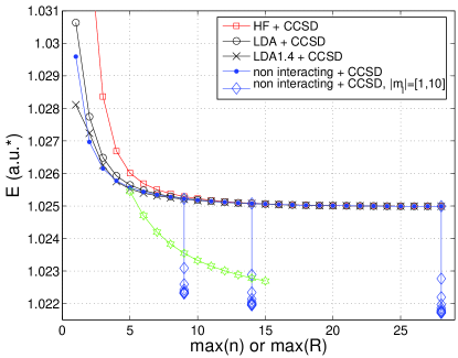
Figure 1: The figure shows the $n$-convergence of the two-particle ground state energy for a dot with a confining potential corresponding to $\hbar\omega=3.32$meV. The $n$-convergence is studied for a variety of starting points in the CCSD-calculation. The maximum $n$- value is varied from $1$ to $28$, while $|m_{l}|\leq 1$ for a Hartree-Fock starting point (red), different Local Density starting points (black), and a non-interacting starting point (blue with solid circles). The vertical lines with diamonds for max$(n)=9,14$ and $28$ show the $|m_{l}|$-convergence with max$(|m_{l}|)=[1,10]$. For reference we note that the energy using second order perturbation theory on top of Hartree Fock is $1.045$ a.u.* when using the basis size $(n,|m_{l}|)\leq(28,1)$. The (green) curve with hexagram markers shows the $R=2n+|m_{l}|$-convergence when starting from the non-interacting basis set.

A strict limitation with the CCSD approach is the neglect of true triples, $S_{3}$ clusters, and beyond. For sufficiently weak confinements this approximation will dominate the error. Table 2 shows a comparison between the CCSD and FCI methods for three and six electrons and for a large range of confinement strengths. The purpose is here to establish how important the limitation to $S_{1}$ and $S_{2}$ clusters is. Confinement strengths as weak as possible, but still leading to a converged coupled-cluster expansion with a non-interacting basis have been used. We note that for $\lambda\leq 1$ the CCSD-method yields results accurate enough for most practical purposes. For $\lambda=2$ the error due to the neglected effects in the CCSD-method is still so small that (keeping table 1 in mind) the possibility to use larger basis sets than in a CI calculation well compensates for the lack of triples and beyond. For $N=3$ and $\lambda=4$ the CCSD did not converge for the $|2SM_{L}1\rangle=|11\rangle$ ground state. For this weak confinement the first excited state is still reproduced well. Generally we see that this first excited state, which is not as localized as the ground state, is reproduced better than the ground state throughout the list of confinements strengths in Table 2 . Intuitively this makes sense; true triple excitations (and all many-body effects) should be relatively more important for more localized states.

IV.2 Convergence of the basis and the use of different starting points

Fig. 1 depicts the basis set convergence for the $N=2$ ground state using different starting points. The potential strength $\hbar\omega=3.32$ meV, corresponding to $\lambda\approx 1.89$, is chosen to enable comparison with the Quantum Monte Carlo results from Ref. Pederiva et al. (2003), where it is argued that this value is close to the actual values in the experiment by Tarucha et al. Tarucha et al. (1996). Fig. 1 shows that the basis sets begin to saturate around max$(n)=10$ and for the angular quantum number they saturate to the same extent at approximately $|m_{l}|=4$. The shell truncation parameter $R=2n+|m_{l}|$, used in most of the previous CI-calculations, is thus here ($N=2$ and $\hbar\omega=3.32$ meV) clearly overemphasizing the need for high $|m_{l}|$-values in the basis set, on the expense of $n$-values. To put it in other words; it is apparent from the figure that a basis cut of $(n,|m_{l}|)\leq(10,4)$ is a better choice than e.g. $R=2n+|m_{l}|\leq 10$. For weaker confinements and more confined particles the behavior is probably different; one expects then the high $|m_{l}|$ basis functions to be relatively more important.

Moreover, Fig. 1 shows that for small $n$ the different starting points give quite a spread in the energy but for n$>10$ the results are virtually independent of the starting point. Again this demonstrates that for the comparison with CI-results from Refs. Kvaal (2009a); Merlot (2009); Massimo Rontani (2006), which all are limited to very few $n$:s, we are limited to the use of the non-interacting starting point. This is unfortunate since the CCSD method can handle much weaker confinement strengths with a Hartree-Fock or a Local Density Starting point.

It is easy to be mislead by Fig. 1 and draw the conclusion that there is no need for other starting points than the pure harmonic oscillator basis and that Hartree-Fock is the worst of the tested starting points. However, the number of needed iterations in Eq.(29 - 30)($\sim$ orders in the perturbation expansion) to obtain self-consistency can differ significantly between the starting points, with Hartree-Fock often being the fastest of them all. For example, with a basis size of $(n,|m_{l}|)\leq(28,1)$ and including up to second order corrections to the energy, the pure harmonic oscillator starting point yields $0.9223$ a.u.*, while Hartree-Fock gives $1.0449$ a.u.* and the fully converged result is $1.0250$ a.u.* (for both starting points). That is, with the Hartree-Fock basis we start much closer to the fully correlated situation.

IV.2.1 Extrapolation and convergence of the basis

Even though much larger basis sets can be used with CCSD than with CI, the calculation time still grows with the number of particles and with the size of the basis set. Extrapolation of the results to infinitely large basis sets is then often an efficient strategy. Many elaborate strategies can be envisaged here, e.g. adjusting the size of the basis set during the iterations. One can for example obtain convergence in a limited basis and then systematically increase it, or one can filter the contributions and only keep those that are estimated to contribute over a certain level. Here we restrict ourselves to a brief discussion of the potential gain of extrapolation.

Table 3: The $|m_{l}|$-convergence (using all $n$, in this case $n\leq 29$) of the two electron ground state energy given in a.u.*. The extrapolated values are found according to the procedure described in the text. The extrapolated values agree well with the values 1.02164(1) and 1.02165(1) by Pederiva et al Pederiva et al. (2003) obtained through Variation Monte Carlo and Diffusion Monte Carlo methods respectively. For each extrapolated value three points were used in the linear fit.

$|m_{l}|$	E($|m_{l}|$)	$|m_{l}|\rightarrow\infty$	Upper bound	Lower bound
1	1.024993	-	-	-
2	1.022767	-	-	-
3	1.022196	1.021703	1.022196	1.021210
4	1.021971	1.021667	1.021971	1.021363
5	1.021861	1.021661	1.021861	1.021461
6	1.021799	1.021660	1.021800	1.021520
7	1.021762	1.021660	1.021762	1.021558
8	1.021737	1.021661	1.021738	1.021584
9	1.021721	1.021661	1.021721	1.021601
10	1.021709	1.021662	1.021709	1.021614

Table 4: The $R=2n+|m_{l}|$-convergence for the $2-8$ electron ground states for a confining potential corresponding to $\hbar\omega=3.32$ meV. The results are given in a.u.*

$R$	2e-	3e-	4e-	5e-	6e-	7e-	8e-
5	1.02544	2.24045	3.72652	5.55317	7.62640	10.0913	12.8065
6	1.02470	2.23924	3.72439	5.54890	7.61942	10.0624	12.7284
7	1.02420	2.23846	3.72210	5.54629	7.61496	10.0541	12.7132
8	1.02383	2.23791	3.72207	5.54454	7.61207	10.0498	12.7067
9	1.02355	2.23750	3.72140	5.54327	7.61000	10.0469	12.7027
10	1.02333	2.23719	3.72089	5.54234	7.60846	10.0448	12.7000
11	1.02315	2.23694	3.72050	5.54161	7.60728	10.0431	12.6979
12	1.02301	2.23674	3.72018	5.54102	7.60633	10.0419	12.6962
13	1.02289	2.23657	3.71991	5.54054	7.60557	10.0408	12.6949
14	1.02278	2.23643	3.71969	5.54014	7.60493	10.0400	12.6939
15	1.02269	2.23631	3.71950	5.53979	7.60438	10.0393	12.6930
QMC	1.02165(1)	2.2395(1)	3.7194(1)	5.5448(1)	7.6104(1)	10.0499(1)	12.7087(1)
QMC	1.02164(1)	2.2339(1)	3.7145(1)	5.5338(1)	7.6001(1)	10.0342(1)	12.6900(1)

A first example is shown in Table 3, where the full radial basis is used to investigate the $m_{\ell}$ expansion. The extrapolated values are obtained through a linear regression fit assuming the relation

$$\ln\left[E(|m_{\ell}|+1)-E(|m_{\ell}|)\right]=K\ln(|m_{\ell}|+1)+C,$$ (32)

where $E(|m_{\ell}|)$ is the energy with the one particle basis cut at $\textrm{max}(|m_{\ell}|)=|m_{\ell}|$ and $K$ and $C$ are the constants we find from the fit. The fits were made with three consecutive differences at a time, which give the list of predictions displayed in the third column in Table 3. It is clear that this procedure can improve the results substantially, especially when a rather low maximum $|m_{\ell}|$ is used. The upper (lower) bound decreases (increases) monotonically as $|m_{l}|$ increases and the extrapolated values stabilize around $1.02166$ a.u.*. This result agrees well with those obtained by Pederiva et al Pederiva et al. (2003), $1.02164(1)$ and $1.02165(1)$ a.u.*, through variational and diffusion quantum Monte Carlo methods respectively.

Table 4 shows the convergence of the ground state energies for two to eight confined electrons as functions of $R=2n+|m_{l}|$. This truncation scheme is a common choice in numerical studiesMassimo Rontani (2006); Kvaal (2009a), and the motivation to study convergence as a function of this parameter is that the energy levels of a non-interacting two-electron dot are given by $\epsilon_{nm_{\ell}}=(2n+|m_{\ell}|+1)\hbar\omega$. The confining potential corresponds to $\hbar\omega=3.32$ meV, a strength that previously has been studied with Quantum Monte Carlo MethodsPederiva et al. (2003), which are shown in the Table for comparison. A comparison with the two-electron results from Table 3 indicates though that the radial convergence is substantially slower than the angular convergence, at least for this confinement strength. For more than two particles the angular convergence slows down due to the mutual repulsion felt by the electrons and the resulting spread of the total wave function. This makes $R$ a reasonable parameter for the truncation of the basis. We emphasize that we have used considerably higher $R$ and/or more confined electrons than used in the available CI calculationsKvaal (2009a); Massimo Rontani (2006). The error relative to the Diffusion Monte Carlo method (expected to be the more accurate of the twoPederiva et al. (2003)) is $\sim 10^{-3}$ and on the same level or below as the difference between the two different Monte Carlo methods. For most purposes so far this would, we believe, be a good enough convergence. We stress that the complete series of $R=[5,15]$ for $N=8$ still did not take more than $\sim 24$ hours to compute on a standard desktop machine, which implies that further converged results can be obtained if necessary.

Table 5: The ground state energy of the $\hbar\omega=3.32$ meV two-electron dot obtained with an alternative extrapolation scheme: Aitken’s $\delta^{2}$-process is used on the $n=7,8$ and $9$ values for respective $|m_{l}|$ to accelerate the $n$-convergence. Subsequently the $|m_{l}|\rightarrow\infty$ extrapolation is done as described in the text. The results are given in a.u.^∗.

$|m_{l}|$	E($|m_{l}|$)	$|m_{l}|\rightarrow\infty$	Upper bound	Lower bound
1	1.025029	-	-	-
2	1.022809	-	-	-
3	1.022232	-	-	-
4	1.022001	1.021697	1.021731	1.021658
5	1.021893	1.021703	1.021719	1.021687
6	1.021839	1.021734	1.021737	1.021697

However, it seems to be very difficult to improve the $R$-cut results through extrapolation. All our attempts so far have resulted in quite unreliable predictions. For example, the extrapolated values did not stabilize, but showed a monotonously decreasing behavior. Instead we have investigated a third possible truncation scheme. In this scheme we have first used the Aitken’s $\delta^{2}$-process, see e.g. Ref. Press et al. (1993), to speed up the convergence in $n$. After that we extrapolate to infinity in $|m_{l}|$ as described at the beginning of this subsection in connection with Table 3. The results for the two-electron dot are displayed in Table 5, where values for $n=7,8$ and $9$ for each $|m_{l}|-$value were used to perform Aitken’s convergence acceleration. In contrast to the attempted $R$-extrapolation, the extrapolated values do now stabilize, and the obtained value $1.0217$ a.u.* is very close to the result obtained in Table 3 using a much larger basis set. The usage of this or similar extrapolation schemes for more than two confined particles is an interesting topic for future studies.

V Conclusions

In conclusion, by comparison with results obtained with Full Configuration Interaction and two different Quantum Monte Carlo methods the Coupled Cluster Singles and Doubles approach is shown to be a very powerful method for two to eight electrons confined in a two-dimensional harmonic oscillator potential. For $\lambda\leq 1$ ($\hbar\omega\approx 11.857$meV for GaAs material parameters) the results are for practical purposes exact when comparing with FCI and for $\lambda=2$ ($\hbar\omega\approx 2.964$meV for GaAs material parameters) the error is still never larger than $\sim 1.5\times 10^{-2}$ in units of $\hbar\omega$. For $N\geq 6$ the possibility to use much larger basis sets than in FCI-calculations is shown to be of uttermost importance. The errors introduced by truncating the basis sets in FCI-calculations are in many cases much larger than the error made by truncating some of the triple and quadruple excitations as done in CCSD. Moreover, when comparing with a Diffusion Monte Carlo study, for a potential strength close to what is estimated from the experiment by Tarucha et al.Tarucha et al. (1996), the errors in the two to eight electron ground states are shown to be on the same level or less than the differences between Variational and Diffusion Monte Carlo results. This gives promise that the method, in future studies, can be used for the extraction of reliable information from experiments.