A Sino-German $\lambda$6 cm polarization survey of the Galactic plane

Abstract

Context. Linearly polarized Galactic synchrotron emission provides valuable information about the properties of the Galactic magnetic field and the interstellar magneto-ionic medium, when Faraday rotation along the line of sight is properly taken into account.

Aims. We aim to survey the Galactic plane at $\lambda$6 cm including linear polarization. At such a short wavelength Faraday rotation effects are in general small and the Galactic magnetic field properties can be probed to larger distances than at long wavelengths.

Methods. The Urumqi 25-m telescope is used for a sensitive $\lambda$6 cm survey in total and polarized intensities. WMAP K-band (22.8 GHz) polarization data are used to restore the absolute zero-level of the Urumqi $U$ and $Q$ maps by extrapolation.

Results. Total intensity and polarization maps are presented for a Galactic plane region of $129\degr\leq\ell\leq 230\degr$ and $|b|\leq 5\degr$ in the anti-centre with an angular resolution of $9\aas@@fstack{\prime}5$ and an average sensitivity of 0.6 mK and 0.4 mK $\rm T_{B}$ in total and polarized intensity, respectively. We briefly discuss the properties of some extended Faraday Screens detected in the $\lambda$6 cm polarization maps.

Conclusions. The Sino-German $\lambda$6 cm polarization survey provides new information about the properties of the magnetic ISM. The survey also adds valuable information for discrete Galactic objects and is in particular suited to detect extended Faraday Screens with large rotation measures hosting strong regular magnetic fields.

1 Introduction

Surveys of the Galactic plane at several frequencies are required to disentangle the individual star formation complexes, or thermal H II regions, non-thermal supernova remnants (SNRs) and extragalactic sources. The diffuse emission associated with the Galactic disk is produced by relativistic electrons spiraling in magnetic fields and by thin ionized thermal gas. Both the diffuse non-thermal emission and the SNRs have significant linear polarization. Mapping of the Galactic plane at several radio frequencies including linear polarization offers a method to separate these non-thermal components as well as allowing a delineation of the Galactic magnetic field.

The Galactic plane has been surveyed from 22 MHz up to 10 GHz, albeit usually without polarization measurements. Sensitive Galactic polarization plane surveys began in the 1980s. A 2.7 GHz survey using the Effelsberg 100-m telescope by Junkes et al. (1987) showed a section of the Galactic plane with $4\aas@@fstack{\prime}3$ angular resolution. Further Northern sky Galactic plane surveys at 2.7 GHz (Reich et al. 1990; Fürst et al. 1990; Duncan et al. 1999) were complemented by 2.4 GHz Southern Galactic plane surveys using the Parkes 64-m telescope (Duncan et al. 1995, 1997). To achieve angular resolution of arc minutes at lower frequencies synthesis radio telescopes had to be used for surveys: e.g. the Westerbork Synthesis Radio Telescope at 350 MHz (Wieringa et al. 1993; Haverkorn et al. 2003a, b), the Dominion Radio Astrophysical Observatory synthesis telescope at 408 MHz and 1.4 GHz (Canadian Galactic Plane Survey, CGPS) (Taylor et al. 2003), and the Australian Telescope Compact Array at 1.4 GHz (Southern Galactic Plane Survey, SGPS) (Gaensler et al. 2001; Haverkorn et al. 2006). Most of the mentioned surveys only cover a narrow strip along the Galactic plane. To overcome this deficiency the Galactic plane was mapped at 1.4 GHz with the Effelsberg 100-m telescope for $|b|\leq 20\degr$. First maps from this survey were shown by Uyanıker et al. (1999) and by Reich et al. (2004). To study the nature of sources and the properties of the magnetic field, polarization surveys at higher radio frequencies are needed. Valuable information about diffuse polarized Galactic emission was provided by WMAP at 22.8 GHz and higher frequencies (Hinshaw et al. 2009), although the angular resolution of $50\arcmin$ at 22.8 GHz is in general too coarse to resolve the complex Galactic structures in the Galactic plane.

The Sino-German $\lambda$6 cm survey, covering a 10$\degr$ wide strip of the Galactic plane, has been carried out since 2004 using the 25-m radio telescope of the Urumqi Observatory, National Astronomical Observatories, CAS. This survey fills the existing gap in frequency coverage by providing maps of the Galactic plane from $10\degr\leq\ell\leq 230\degr$ and $|b|\leq 5\degr$ with an angular resolution of $9\aas@@fstack{\prime}5$. The survey maps and a list of compact sources will be released after completion of the $\lambda$6 cm survey project expected for the end of 2010. The first results have already been presented by Sun et al. (2007) (hereafter called Paper I), including details of the survey concept, the observing and calibration methods and the reduction process. In Paper I, covering the longitude range from $122\degr$ to $129\degr$, we illustrated the scientific potential provided by the $\lambda$6 cm survey by delineating new faint H II regions, studied spectra of SNRs, discovered Faraday Screens as well as traced the magnetic fields in this section of the Galactic plane. Most remarkable discoveries are two extended Faraday Screens located at the Perseus arm. One of them is caused by a previously unknown faint H II region. Both Faraday Screens host strong regular magnetic fields with rotation measures ($RM$) of the order of 200 rad m^-2. They are not visible at low frequencies because such high $RM$s cause a polarization angle rotation by more than $180\degr$, or they are beyond the polarization horizon. This proves the value of a sensitive $\lambda$6 cm polarization survey to detect them in the magnetized interstellar medium. The commonly adopted picture of the Galactic magnetic field in the thin disk to consist of a regular component following basically the spiral arms of the Galaxy together with a turbulent magnetic field component of about similar strength might be modified in case numerous extended Faraday Screens with a uniform regular magnetic field exist. The origin of such magnetic bubbles acting as Faraday Screens is not clear so far.

Here we present the second section of the $\lambda$6 cm survey for the outer Galaxy covering the region $129\degr\leq\ell\leq 230\degr$. In Sect. 2 observation and data processing details for this survey area are discussed. In Sect. 3 we present the total power and polarization maps (Sect. 3.1), followed by a brief discussion on the survey’s potential to study and detect SNRs (Sect. 3.2) and H II regions (Sect. 3.3), while in Sect. 3.4 we focus on newly detected and prominent Faraday Screens in the interstellar medium. Results are summarized in Sect. 4.

2 Observations and Data reduction

2.1 Observation set-up

The Sino-German $\lambda$6 cm polarization survey of the Galactic plane was carried out with the 25-m Urumqi telescope. The $\lambda$6 cm system is a copy of an Effelsberg single-channel receiver and has a system temperature of about 22 K when pointing to the zenith at clear sky. The half-power beam width (HPBW) of the telescope was $9\aas@@fstack{\prime}5$. Survey observations were exclusively made during clear sky at night time. In “broad band mode” the centre frequency was 4800 MHz with a bandwidth 600 MHz, while in “narrow band mode” the centre frequency was 4963 MHz with a bandwidth of 295 MHz. “Narrow band mode” was used to avoid contamination by the geostationary Indian INSAT-satellites located at four positions in southern and western directions, which emit strong signals below frequencies of about 4810 MHz. Thus all observations close to the satellite positions were made in “narrow band mode”, while the “broad band mode” was used for all other directions. The survey region was limited at $\ell=230\degr$, because regions with larger $\ell$ have to be observed at very low elevations, so that the increased ground radiation can not be subtracted with sufficient accuracy. Measurements of the ground radiation properties of the Urumqi 25-m telescope at $\lambda$6 cm were already reported by Wang et al. (2007). The main observational survey parameters are listed in Table 1.

Survey maps were observed in two orthogonal directions: along $\ell$ and $b$. The combined survey consists of a large number of individual 8$\degr\times 2\aas@@fstack{\circ}6$ or $8\aas@@fstack{\circ}2\times 2\aas@@fstack{\circ}6$ maps observed in $\ell$ direction and of $2\degr\times 10\degr$ or $2\aas@@fstack{\circ}2\times 10\degr$ maps observed along $b$. Total intensity, Stokes $I$, and the linearly polarized components, Stokes $U$ and $Q$, were measured simultaneously. 3C286 and 3C295 served as the main polarized and un-polarized calibration sources, while 3C48, 3C138 served as secondary polarized calibrators. Calibration sources were always observed before starting a survey map in the same observation mode.

We increased the original scanning speed of the observations from $2\aas@@fstack{\circ}5$/min to $4\degr$/min after tests performed in 2006. The reason was to minimize the influence of system instabilities and also the contamination by changing ground radiation and low-level RFI. To achieve the same S/N ratio we thus mapped the same region more often. The sensitivity is not unique throughout the entire survey section, since the coverages of $\ell$ and $b$ maps differ. The effective integration time of each map pixel is at least 2.6 sec for total intensity and 1.9 sec for polarization, where the integration time of map pixel observed in “narrow band mode” were divided by a factor of 2 to be comparable with that of “broad band mode”. The effective integration time of each sub-region in Stokes $I$, $U$ and $Q$ for 600 MHz bandwidth is shown in Fig. 1.

Table 1: Observational parameters

System Temperature	22 K $\rm T_{a}$
HPBW	$9\aas@@fstack{\prime}5$
Subscan separation, sampling	3$\arcmin$
Scan velocity	2$\aas@@fstack{\circ}$5/min or 4°/min
Scan direction	$\ell$ and $b$
Typical rms-noise for $I$	0.5 - 0.7 mK $\rm T_{B}$
Typical rms-noise for $U$ and $Q$	0.3 - 0.4 mK $\rm T_{B}$
Typical rms-noise for $PI$	0.3 - 0.5 mK $\rm T_{B}$
Central frequency	4800 MHz or 4963 MHz
Bandwidth	600 MHz or 295 MHz
aperture efficiency	62%
beam efficiency	67%
TB/S	0.164 K/Jy
Main Calibrator	3C286
Flux density	7.5 Jy
Percentage Polarization	11.3%
Polarization Angle	33°

2.2 Data reduction

Data reduction was done following the standard procedures, which were already described in Paper I. Subsequently the following steps are applied: For total intensity $I$ maps, a baseline was appropriately fitted for each sub-scan, which implies that large-scale diffuse emission exceeding the length of the sub-scans of $8\degr$ or $10\degr$ is not preserved. In addition, spiky pixels were removed, distorted sub-scan sections or entire sub-scans were set to dummy values or, for smooth regions, replaced by interpolation of the two neighboring sub-scans. The baselines of the Stokes $U$ and $Q$ maps were usually not fitted in order to preserve extended polarized emission, unless strong ground radiation at low elevations clearly contaminates the data. Baseline distortion effects along scanning direction were suppressed by the “unsharp masking” method (Sofue & Reich 1979). Spiky pixels and bad sub-scans were corrected in the same way as the $I$ maps. We noted that afterwards many maps show residual distortions visible as inclined stripes, which seem to be caused by RFI-sources of unknown origin. They were well removed by rotating the map that the stripes align to rows or columns of the map to apply the “unsharp masking” procedure and then rotating the map back.

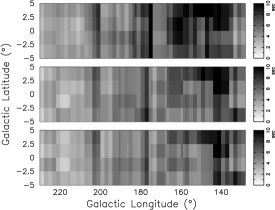
Figure 1: Distribution of effective integration time in sec for the survey sub-areas shown for Stokes $I$, $U$ and $Q$ from top to bottom.

Total intensity and polarization calibration was based on 3C286 (see Table 1). Instrumental polarization from strong sources was removed by the “REBEAM” procedure of the NOD2 package as described in Paper I. This method reduces the ringlike instrumental response in polarized intensity $PI$ by about 50%, which leaves some residual instrumental response of the order of 1%. Our sensitivity limit on average (3 $\times$ rms) is 1.2 mK $\rm T_{B}$ (or 7.3 mJy/beam). Only strong sources exceeding about 0.7 Jy will show weak polarization response of instrumental origin, which will, however, in most cases confuse with diffuse Galactic emission.

Compact sources of the NVSS catalogue (Condon et al. 1998) were used to check the position accuracy. Finally, all individually edited maps were combined by applying the “PLAIT”-algorithm (Emerson & Gräve 1988), where the Fourier transforms of the maps were added and the final map is obtained by an inverse Fourier transform. “PLAIT”, in addition, is able to suppress remaining low-level scanning effects still visible in a few individual maps.

2.3 Absolute zero-level restoration for Stokes $U$ and $Q$

We have observed scans of up to 10$\degr$ in length aiming to recover extended structures as large as possible. All maps have a relative zero-level by arbitrarily setting the edge values of each scan to zero. Total intensity maps (Stokes $I$) always miss a positive temperature offset, while the offsets for Stokes $U$ and $Q$ maps may be positive or negative. Polarized intensity, $PI$, of unknown intensity originating from Faraday rotated diffuse emission in the interstellar medium may exist everywhere and is not related to total intensity. Thus the true zero-level of the observed $U$ and $Q$ maps remains unknown. Therefore $PI$ and the polarization angle, $PA$, as calculated from $U$ and $Q$, need to be corrected as well. We note that relative polarization zero-level setting may be done in different ways, e.g. setting the mean value of $U$ and $Q$ of each scan to zero (Junkes et al. 1987). After we combined maps observed along $\ell$ direction with maps along $b$ direction, the edge areas of the final combined maps differ from zero.

Since polarized components are vectors, a missing large-scale component may lead to a misinterpretation of the observed data (Reich 2006). This is in particular important for polarized emission resulting from Faraday rotation, which clearly dominates the Galactic polarization maps at $\lambda$6 cm. In Paper I, Sun et al. (2007) already presented a solution for this problem by adopting the three-year K-band (22.8 GHz) polarization data from WMAP (Page et al. 2007), which have a correct zero-level. Missing large-scale $U$ and $Q$ emission at $\lambda$6 cm is restored by scaling the K-band data by a factor of $(4.8/22.8)^{-2.8}$, according to a temperature spectral index of $\beta=-2.8$. This procedure also assumes that the $RM$ of the diffuse emission is not significant.

For this second much larger section of the $\lambda$6 cm polarization survey we slightly modified the method applied in Paper I by taking meanwhile available additional information into account. We now use the five-year release of the WMAP observations (Hinshaw et al. 2009). We calculated the spectral index distribution between the polarized emission at 1.4 GHz (Wolleben et al. 2006) and the K-band data for the entire survey section, smoothed to a common angular resolution of 2$\degr$. We obtained a mean spectral index of $\beta=-2.92\pm 0.25$. We note that this spectral index is largely biased by the dominating polarized emission from the bright Fan-region, which is Faraday thin at 1.4 GHz. This, however, is likely not the case for the Galactic plane emission at 1.4 GHz from large distances. Current estimates of the synchrotron total intensity spectrum quote very similar spectral values between 1.4 GHz and 23.8 GHz (see Dickinson et al. (2009) for a recent discussion), which we expect to be valid for the extrapolation of Faraday thin diffuse large-scale polarized emission from 22.8 GHz to 4.8 GHz as well.

We compared the WMAP K-band (22.8 GHz) and Ka-band (33 GHz) polarization data (Hinshaw et al. 2009) at 2$\degr$ angular resolution for common extended polarization structures in the present survey area. Clearly, the vast majority of patchy, weak polarization features in the two WMAP maps were not correlated and thus do not show patches of polarized emission. This in turn means that an extrapolation of the polarized K-band emission towards $\lambda$6 cm becomes questionable as it might introduce spurious features specific to the K-band map. Large-scale polarization gradients, however, are common in the K-band and Ka-band maps. We therefore decided to convolve the $\lambda$6 cm $U$ and $Q$ survey maps and the corresponding K-band maps to 2$\degr$ angular resolution after having removed a few strong and compact polarized sources, The convolved maps were split into sections, scaled by a factor of $(4.8/22.8)^{-2.9}$ and the difference values in their corner areas were determined. These difference values were used to define correction hyper planes in $U$ and $Q$ for each $\lambda$6 cm survey section and were applied to the data at their original resolution. In Table 2 we list the $U$ and $Q$ intensities of the Urumqi observations and the corresponding scaled K-map values together with the resulting correction values. The maximum error introduced by assuming a constant spectral index of $\beta=-2.9$ will occur at $\ell=129\degr$ and is estimated to be about $\pm$1.5 mK $\rm T_{B}$ in case the assumed spectral index varies by $\Delta\beta=\pm$0.1.

A significant $RM$ will change the extrapolated corrections for $U$ and $Q$, while $PI$ remains unchanged. Numerous $RM$s from extragalactic sources in the Galactic plane are available (Brown et al. 2007). On average high $RM$-values are observed in the surveyed area with a clear gradient along $\ell$, but also a significant scatter of $RM$ is noted. However, it is known that the $RM$ of diffuse polarized Galactic emission in this area is small (Spoelstra 1984; Haverkorn et al. 2003b). We used the recent 3D-model of Galactic emissivities by Sun et al. (2008), which is in agreement with observed $RM$s, to model the polarized emission distribution at 4.8 GHz and 22.8 GHz. The distribution of $RM$ was obtained from the $PA$ maps at both frequencies. The $RM$ map shows small values in general, as expected, and a nearly linear increase of $RM$ from $\ell=129\degr$ to 230$\degr$. For $\ell=129\degr$, $b=+5\degr,0\degr$ and $-5\degr$ the simulations predict $RM$ values of $-18$, $-35$ and $-25$ rad m^-2 . For $\ell=230\degr$ the $RM$ values are $+31$, $+66$ and $+38$ rad m^-2, respectively. The simulations by Sun et al. (2008) did not take into account the excessive polarized emission from the so-called ”Fan”-region, a discrete very extended and highly polarized structure, which clearly dominates the large-scale polarized emission for $\ell$ lower than about $160\degr$. The “Fan”-region is known to have $RM$s very close to zero at low angular resolution (Spoelstra 1984). Thus no $RM$ based correction for the low $\ell$ end of the observed area is necessary. The maximum $RM$ of 66 rad m^-2 at $\ell=230\degr,b=0\degr$ means a $PA$ change between 4.8 GHz and 22.8 GHz of 14$\degr$. Such an angle difference should be taken into account. However, the zero-level corrections for $U$ and $Q$ in this area (see Table 2) are below the 3 $\times$ rms-noise in $U$ and $Q$ of the observations, so that we neglect the $RM$ effect on the $U$ and $Q$ corrections.

The effect of the zero-level restoration process is illustrated in Fig. 2 by comparing the distributions of $PI$ and $PA$ before and after the large-scale correction. Both distributions are clearly changed. In particular, $PA$ changed from an almost uniform distribution between $-90\degr$ and $+90\degr$ into a distribution with a clear maximum for $PA$ near 0$\degr$ for the restored data, reflecting the fact that significant large-scale corrections are required for Stokes $Q$, while $U$ remains almost unchanged. This means that on large scales the magnetic field is orientated along $\ell$ (PA = 0$\degr$).

Figure 2: Pixel distribution for $PI$ (top) and $PA$ (bottom) before and after restoring missing large-scale structures extrapolated from WMAP K-band. Details are discussed in Sect. 2.3.

Table 2: Hyper plane corrections in mK $\rm T_{B}$

$\ell$	$b$	U	U	U	Q	Q	Q
(deg)	(deg)	6 cm	Kmap	corr	6 cm	Kmap	corr
$230.0$	$+5.0$	$0.0$	$0.0$	$0.0$	$-0.1$	$0.5$	$0.6$
$210.5$	$+5.0$	$-0.1$	$-0.5$	$-0.4$	$-0.1$	$0.7$	$0.8$
$188.0$	$+5.0$	$-0.6$	$-0.4$	$0.2$	$0.2$	$1.8$	$1.6$
$167.5$	$+5.0$	$-0.3$	$-1.5$	$-1.2$	$0.6$	$4.1$	$3.5$
$148.5$	$+5.0$	$-0.2$	$-0.3$	$-0.1$	$0.2$	$8.2$	$8.0$
$129.0$	$+5.0$	$0.5$	$0.6$	$0.1$	$0.6$	$10.1$	$9.5$
$230.0$	$-5.0$	$-0.5$	$-0.6$	$-0.1$	$0.0$	$2.3$	$2.3$
$210.5$	$-5.0$	$-0.2$	$-0.5$	$-0.3$	$0.0$	$3.0$	$3.0$
$188.0$	$-5.0$	$-0.2$	$-1.3$	$-1.1$	$0.1$	$5.4$	$5.3$
$167.5$	$-5.0$	$0.1$	$-1.0$	$-1.1$	$-0.1$	$5.7$	$5.8$
$148.5$	$-5.0$	$-0.1$	$0.7$	$0.8$	$-0.6$	$8.5$	$9.1$
$129.0$	$-5.0$	$-0.1$	$0.3$	$0.4$	$-0.4$	$10.2$	$10.6$

3 Analysis of the survey region

Large-scale emission seen in the present $\lambda$6 cm survey section originates from the local arm, the Perseus arm and probably an outer arm (Hou et al. 2009). Also emission contributed from the inter-arm regions is possible. A large number of extended and compact sources are also visible in the surveyed area. The total intensity $I$ maps very well resemble the emission structures visible in surveys at longer wavelengths with similar angular resolution, e.g. the Effelsberg surveys at $\lambda$21 cm (Kallas & Reich 1980; Reich et al. 1997) and at $\lambda$11 cm (Fürst et al. 1990). The $\lambda$6 cm polarization data, however, show rather different structures compared to partly available Effelsberg $\lambda$21 cm survey data (Uyanıker et al. 1999; Reich et al. 2004) and are therefore of particular interest, so that we focus on them in the following.

Compact or slightly resolved sources of the entire $\lambda$6 cm Urumqi survey will be listed in a separate paper after completion of the survey. Several prominent sources like the Cygnus Loop (Sun et al. 2006), OA184 (Foster et al. 2006), the SNRs G156.2+5.7 (Xu et al. 2007), S147 (Xiao et al. 2008), HB3 (Shi et al. 2008b), and G65.2+5.7 (Xiao et al. 2009) were already studied in detail based on observations made with the Urumqi $\lambda$6 cm system, which prove the high quality of the data. Data of three newly identified H II regions from the present survey region were published by Shi et al. (2008a). We will present a discussion of other SNRs, H II-regions and prominent extended emission complexes in subsequent papers.

3.1 The survey maps

We show the maps of the outer Galactic plane in four parts (Part 1 to Part 4) in Figs. 3 to 6. The maps have an overlap in $\ell$ of $1\degr$. We show Stokes $I$, $U$ and $Q$ maps as observed with the Urumqi 25-m telescope. In addition, we show maps of $PI$, which were calculated from the $U$ and $Q$ maps but with the large-scale hyper plane corrections as discussed in Sect. 2.3. When calculating $PI$ the correction for the positive noise offset: $PI^{2}=U^{2}+Q^{2}-1.2\sigma_{U,Q}^{2}$ (Wardle & Kronberg 1974) was applied, where $\sigma_{U,Q}$ (see Table 1) is the averaged rms-noise for the $U$ and $Q$ maps for a specific survey area. Polarization bars in B-field direction are overlaid on the $PI$ image. The bars indicate the magnetic field direction in case of small Faraday rotation. The sensitivity throughout the surveyed region varies slightly due to different integration time for different parts as outlined in Sect. 2.1 and Fig. 1. In addition smaller $\ell$ sections have in general a higher sensitivity than areas with larger $\ell$, because they benefit from both the “broad band mode” and less contamination by ground radiation.

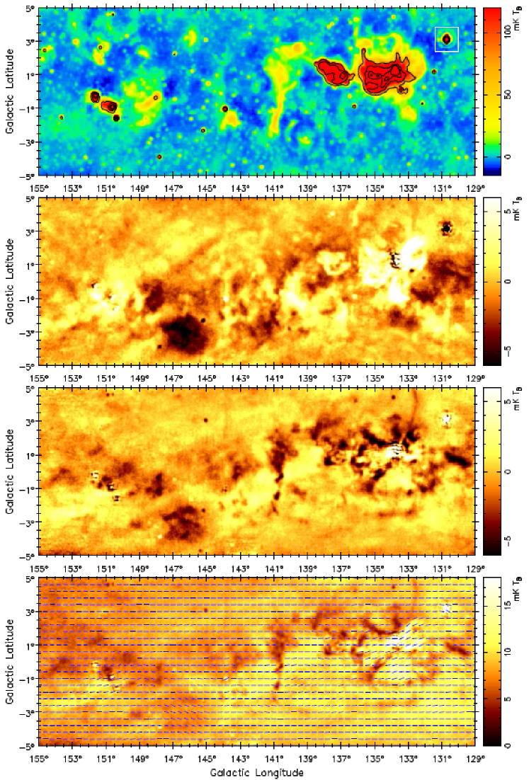
Figure 3: Urumqi $\lambda$6 cm survey maps (Part 1). From top to bottom: Stokes $I$, $U$, $Q$ maps in mK $\rm T_{B}$ as observed and the $PI$ map with large-scale restoration. $I$ contours are shown at 70, 200, 500 and 800 mK $\rm T_{B}$. The $PI$ map is overlaid by polarization vectors in B-field direction, when $PI$ exceeds 6 mK $\rm T_{B}$. Vectors are shown for pixel being 24$\arcmin$ apart in $\ell$ and $b$. Their length is proportional to $PI$. The white rectangle marks the area of SNR 3C58, which is too strong to remove its side-lobes completely.

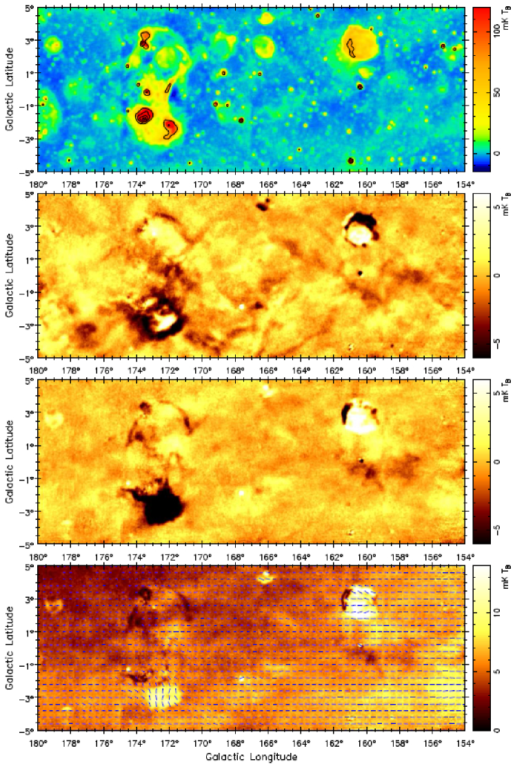
Figure 4: Sequence and contours as in Fig. 3 for Part 2. Vectors are shown for $PI$ exceeding 2.5 mK $\rm T_{B}$.

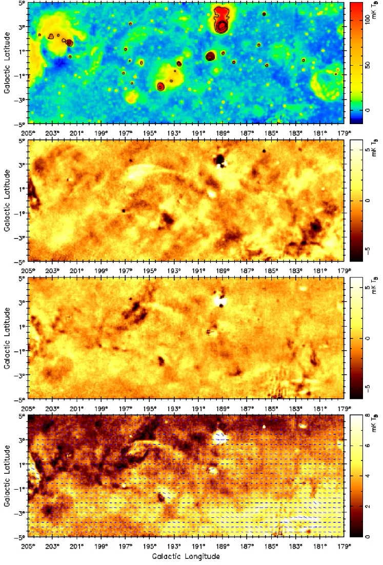
Figure 5: Sequence and contours as in Fig. 3 for Part 3. Vectors are shown for $PI$ exceeding 1.5 mK $\rm T_{B}$.

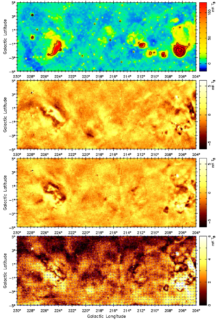
Figure 6: Sequence and contours as in Fig.  3 for Part 4. Vectors are shown for $PI$ exceeding 0.9 mK $\rm T_{B}$.

The survey maps and the compact source list will be made publicly available after completion of the entire project via the MPIfR survey-sampler, the webpage at the National Astronomical Observatories, CAS and possibly other data centres.

3.2 Supernova Remnants (SNRs)

SNRs play an important role for many processes in the interstellar medium, such as energy input, chemical enrichment of heavy elements, cosmic ray production, and thus influence the evolution of galaxies. Most Galactic SNRs are well studied at low radio frequencies, while information about their fainter high-frequency emission is limited. The polarization properties of many SNRs are not well studied at all. Sensitive observations of large SNRs are quite time consuming for large single-dish telescopes at high frequencies because of their small beam-size and the low intensity of SNRs. Observations with interferometers have even higher angular resolution but suffer from missing large-scale components. Our $\lambda$6 cm survey complements high-frequency total power and polarization data for numerous large diameter SNRs.

Eleven known SNRs according to the most recent SNR catalogue (Green 2009) are all visible in the present survey region. Several individual studies of SNRs based on the Urumqi $\lambda$6 cm survey were already published as mentioned above, more are in preparation. The sources HB3, OA184, S147 and the small bottom part of G156.2+5.7 are included in the present survey section. For the first time polarized emission at $\lambda$6 cm is seen for the SNRs HB9 (G160.9+2.6), VRO42.05.01 (G166.0+4.3), the Monoceros Nebula (G205.5+0.9), and PKS0646+06 (G206.9+2.3).

So far we have not unambiguously detected any new SNRs. The surface brightness limit for a SNR with a thick shell according to a 3$\sigma$ detection limit is about $\rm\Sigma_{1GHz}=3.9\ \times 10^{-23}[Wm^{-2}\ Hz^{-1}\ sr^{-1}$] for a temperature spectral index of $\beta=-2.5$. This is lower than that of G156.2+5.7 (Reich et al. 1992), which has the lowest surface brightness in the SNR catalogues.

As an example to show the potential of the Urumqi $\lambda$6 cm survey for SNR research, we discuss the SNR candidate G151.2+2.85, which was proposed by Kerton et al. (2007) based on a steep temperature spectrum ($\beta=-2.75$) of the filamentary structures designated CGPSE 172 and 168 (see their Fig. 5), which are clearly visible at 408 MHz and 1420 MHz in the CGPS (Taylor et al. 2003). These two filamentary structures are aligned and about 1$\degr$ long in total. Both filaments are seen in the $\lambda$6 cm survey and the Effelsberg survey at $\lambda$11 cm (Fürst et al. 1990) and $\lambda$21 cm (Reich et al. 1997). From a TT-plot of $\lambda$6 cm versus $\lambda$21 cm data we obtained temperature spectral indices of $\beta=-2.44\pm 0.08$ and $\beta=-2.34\pm 0.08$ for CGPSE 172 and 168, respectively, larger than those of Kerton et al. (2007). These results clearly confirm the non-thermal nature of these filaments and support the suggestion by Kerton et al. (2007) that the filaments are part of a SNR shell. However, like Kerton et al. (2007) we can not give the entire size and integrated flux density of the SNR shell, because outside the filaments any SNR related emission is too faint, so that it confuses with unrelated Galactic emission. Additional observations, in particular outside of the radio range, are required to trace this object.

3.3 H II regions

Despite of numerous H II region catalogues, in particular that compiled by Paladini et al. (2003), there are many more H II regions to be detected and their physical parameters to be determined. In this survey region many large H II regions have been detected. At $\lambda$6 cm the non-thermal to thermal emission ratio is lower than that at longer wavelengths, so that the detection or isolation of H II regions from diffuse Galactic non-thermal emission including survey data at longer wavelengths in the analysis can be done more easily. We have carefully analyzed the maps and searched for sources with flat spectra and strong infrared emission and found several compact and extended H II regions, previously not catalogued. We also noted that many H II regions have not well defined parameters, which we are able to improve based on the new radio data. The results of this analysis will be presented in forthcoming paper.

3.4 Prominent Faraday Screens

Faraday Screens are magnetized interstellar objects, which do not emit synchrotron emission themselves, but contain a regular magnetic field and thermal electrons causing Faraday rotation. Depending on their physical parameters, Faraday Screens depolarize and rotate polarized background emission, which is observed together with the polarized foreground emission. The observed polarized emission surrounding a Faraday Screen may be either higher or lower than that seen in the Faraday Screen direction, depending on its $RM$ and on the properties of the foreground and background components. Faraday Screens become visible as coherent structures in $PI$ and/or $PA$ maps compared to the diffuse polarized Galactic emission. A proper analysis of Faraday Screens requires the inclusion of polarized structures on all scales. Faraday Screens were already discussed and analyzed in various earlier papers e.g. Wolleben & Reich (2004), Reich (2006), Paper I. Of particular interest are Faraday Screens detected in the $\lambda$6 cm polarization survey maps, since they have larger $RM$s than those at $\lambda$11 cm or $\lambda$21 cm, which might indicate regular magnetic fields with significant strength depending on their thermal electron densities and sizes. If $PA$ is rotated by 180$\degr$ by a Faraday Screen the background remains unchanged except for beam depolarization. This corresponds to a $RM$ exceeding about 70 rad m^-2 at $\lambda$21 cm or 260 rad m^-2 at $\lambda$11 cm, but about 800 rad m^-2 at $\lambda$6 cm. The visibility of Faraday Screens in total intensity just depends on their thermal electron density. Thus we do not distinguish between H II regions and Faraday Screens with no counterpart in total intensity or H$\alpha$ in the following.

3.4.1 Modeling Faraday Screens

A simple model to derive the physical parameters of a Faraday Screen was already introduced in Paper I. The model uses two observed components, marked as “$\mathrm{on}$” and “$\mathrm{off}$”, where “$\mathrm{on}$” is for the position where the line of sight passes the Faraday Screen. Through fitting the Faraday Screen parameters by the observed data, the $RM$ and the depolarization properties of a Faraday Screen can be derived. The polarized background emission, $PI_{bg}$, is the component originating at larger distances than the Faraday Screen, and the polarized foreground emission, $PI_{fg}$, originates in front of the Faraday Screen. The observed “$\mathrm{off}$” component is simply the combined polarized background and foreground emission, while the “$\mathrm{on}$” component is the polarized foreground emission plus the modulated polarized background emission by the Faraday Screen. We assume both components are smooth and have the same $PA$ for the “$\mathrm{on}$” and “$\mathrm{off}$” components. The equations below describe the model, details can be found in Paper I.

$${\left\{\begin{array}[]{cc}\displaystyle\frac{PI_{\mathrm{on}}}{PI_{\mathrm{off}}}=\sqrt{\mathit{f}^{2}(1-c)^{2}+c^{2}+2\mathit{f}c(1-c)\cos 2\psi_{s}}\ ,\\ \displaystyle PA_{\mathrm{on}}-PA_{\mathrm{off}}=\frac{1}{2}\arctan\left(\frac{\mathit{f}(1-c)\sin 2\psi_{s}}{c+\mathit{f}(1-c)\cos 2\psi_{s}}\right),&\end{array}\right.}$$ (1)

here $\mathit{f}$ is the depolarization factor ranging from 0 to 1, where $\mathit{f}$ = 0 indicates total depolarization by the Faraday Screen, while $\mathit{f}$ = 1 means no depolarization. Parameter $c$ is defined as $PI_{fg}/(PI_{fg}+PI_{bg})$.

Note that the model assumes that the $PA$s of the background and foreground emission are in general the same, because the dominating large-scale magnetic field is oriented along the Galactic plane. A model which takes into account different $PA$s for foreground and background emission was presented by Wolleben & Reich (2004), which, however, at least needs observations at two wavelengths. The equations above show the dependence of the observed $PI_{\mathrm{on}}$ and $PI_{\mathrm{off}}$, the $PA_{\mathrm{on}}$ and the $PA_{\mathrm{off}}$ from the modeled foreground $PI_{fg}$ and background $PI_{bg}$ emission components and the Faraday rotation angle $\psi_{s}=RM_{FS}\lambda^{2}$.

Here, $RM_{FS}$ [rad m^-2] = 0.81 $n_{e}$[cm${}^{-3}]\ B_{\parallel}[\mu$G] $l$[pc], with $n_{e}$ being the thermal electron density, $B_{\parallel}$ the field strength of the line-of-sight component of the regular magnetic field and $l$ the line-of-sight length of the Faraday Screen. The size of the source is usually assumed to be that seen in projection. In case the Faraday Screen has measurable thermal emission, $n_{e}$ can be calculated from the emission measure $(EM)$, which is defined as $EM=n_{e}^{2}\ l$. For an optically thin H II region, the observed brightness temperature $T_{B}$ depends on $EM$,

$$T_{B}=8.235\times 10^{-2}\left(\frac{T_{e}}{K}\right)^{-0.35}\left(\frac{\nu}{GHz}\right)^{-2.1}\left(\frac{EM}{pc\ cm^{-6}}\right)a(\nu,T)\ ,$$ (2)

where the correction a($\nu$, T) is taken as 1. The effective temperature $T_{e}$ is always assumed to be 8000 K. Another method to obtain $n_{e}$ depends on the measured H$\alpha$ intensity, which needs to be corrected by the reddening measurement of the exciting star following Haffner et al. (1998):

$$EM=2.75\ T_{4}^{0.9}I_{\rm H\alpha}\exp\ [2.44E(B-V)]\ .$$ (3)

Precise reddening measurements are difficult to obtain.

Prominent extended Faraday Screens seen in this survey section were selected for discussion in the following in order of their $\ell$.

3.4.2 W5 ($\ell=137\aas@@fstack{\circ}6,b=1\aas@@fstack{\circ}1$) and the “lens” Faraday Screen

W3/W4/W5 are prominent H II regions forming a chain together with the SNR HB3 in the Perseus arm about 2 kpc away. Gray et al. (1999) used the DRAO Synthesis Telescope and obtained 1$\arcmin$ resolution radio images of both total intensity and polarized emission of this field at 1.4 GHz. We limit our discussion to W5 in the following. At $\lambda$6 cm $PI$ in this area (Fig. 7) appears to be depolarized by a different amount and the distribution is mottled for our $9\aas@@fstack{\prime}5$ beam, although we see less fine structures when compared to the 1.4 GHz map of Gray et al. (1999).

Heiles (2000) compiled a catalogue of polarized stars and lists nine of them in the vicinity of W5. We calculated a mean $PA$ = 0$\aas@@fstack{\circ}$3$\pm 4\aas@@fstack{\circ}1$ up to the largest distance of 3.6 kpc, where $PA$ runs counter-clockwise with the Galactic plane as reference. The alignment of $PA$ around 0$\degr$ means that the magnetic field is orientated along the Galactic plane for all distances and thus confirms the assumption of our Faraday Screen-model. The $\lambda$6 cm $PA$s in the W5 area, however, vary (Fig. 7) and mottled depolarization is also visible, which is explained by Faraday rotation of different amount.

Westerhout (1958) listed some physical parameters of W5 such as EM = 4000 pc cm^-6 and $n_{e}=10\ cm^{-3}$. From the $\lambda$6 cm brightness temperature of W5 West of about 380 mK $\rm T_{B}$, we calculated a comparable $EM$ value of 2900 pc cm^-6 according to Eq. 2. In addition the H$\alpha$ intensity of W5 can be extracted from the H$\alpha$ full sky map (Finkbeiner 2003) to be about 300 Rayleigh. A reddening measurement of the exciting star $BD+59\aas@@fstack{\circ}0562$, also named Hilt 360 (Hiltner 1956), gives an E(B-V) factor of 0.63. Following Eq. 3, $EM$ can be estimated to be 3140 pc cm^-6, slightly above the radio-based result.

If we take $|B_{\parallel}|=3\ \mu$G as assumed by Gray et al. (1998) as the strength of the line-of-sight component of the regular magnetic field within W5, the expected $|RM_{FS}|$ value is about 970 rad m^-2 for a size of 40 pc and for $n_{e}$ about 10 cm^-3 (Westerhout 1958). This predicts about 217$\degr$ for $\psi_{s}$ at $\lambda$6 cm.

W5 is a large object, where the foreground polarization fraction $c$ may vary across the source. For $c=0.7,0.8$, and $0.9$, and assuming $B_{\parallel}$ and $n_{e}$ to be uniform, we calculate $PI_{\mathrm{on}}/PI_{\mathrm{off}}=84\%,88\%,93\%$ and $PA_{\mathrm{on}}-PA_{\mathrm{off}}=10\degr,6\degr,3\degr$ for the Faraday Screen. As an example, we model $RM_{FS}$ for the fairly uniform W5 East area for an average brightness temperature of about 270 mK $\rm T_{B}$ and a size of $0\aas@@fstack{\circ}7$ corresponding to 24 pc for 2 kpc distance. With $c=0.79$ we calculate $RM_{FS}$ = 260$\pm$60 rad m^-2, which is much smaller than the value estimated for W5 above. This indicates that $B_{\parallel}$ is about 1.5 $\mu$G and $n_{e}$ about 9.2 cm^-3 within W5 East.

Two remarkable polarization features are clearly visible at the edges of W5 in the $\lambda$6 cm polarization map (Fig. 7) at $\ell=137\aas@@fstack{\circ}85,b=0\aas@@fstack{\circ}50$ and at $\ell=136\aas@@fstack{\circ}85,b=1\aas@@fstack{\circ}60$, which resemble Faraday Screens detected at the edges of molecular clouds by Wolleben & Reich (2004). We apply the model fit to the eastern blob. The problem is that we can not definitely decide from single-wavelength data whether $RM_{FS}$ is positive or negative, since the absolute values are very similar. We either obtain $RM_{FS}=-365\pm 30$ rad m^-2 for $c=0.30$ and $\mathit{f}=0.87$ or $RM_{FS}=+350\pm$40 rad m^-2 for $c=0.60$ and $\mathit{f}=0.93$. We show the averaged observed values and the fitted $RM$s in Fig. 8. If the blob is a Perseus arm object like W5, a positive $RM_{FS}$ is preferred, because of the larger $c$ value. Brown et al. (2003b) examined the $RM$ values of extragalactic sources and pulsars in the direction of $105\degr\leq\ell\leq 135\degr$ within the Galactic plane and found that most values are negative. However, Mitra et al. (2003) showed a schematic model (their Fig. 5) that the curvature of the magnetic field lines near H II regions may result in a reverse $RM$ sign. Assuming 2 kpc distance the first three pixels give an average $n_{e}$ of about 4.7 cm^-3 assuming a blob-size of 10.5 pc, and $B_{\parallel}$ is about 8.8 $\mu$G. These parameters clearly differ from the average values obtained for W5. Of course, we could not entirely rule out a projection effect, so that these blobs are seen at the periphery of W5 by chance.

Wolleben & Reich (2004) discovered line-of-sight magnetic field components exceeding 20 $\mu$G at the surface of the local Taurus molecular clouds, which is morphologically quite similar to the W5 polarization blobs seen at $\lambda$6 cm. Note that the uncertainty of the line-of-sight size of the Faraday Screen plays an important role in determining $B_{\parallel}$ and $n_{e}$. A tube-like shaped Faraday Screen would reduce the values of $B_{\parallel}$ and $n_{e}$. To precisely constrain such high $RM$ values, observations at even shorter wavelengths than $\lambda$6 cm are needed, which are, however, difficult to do.

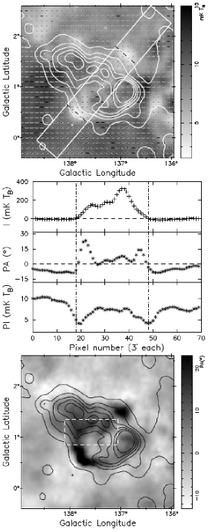
Figure 7: Upper plot shows the $PI$ map of W5 in grey scale, overlaid by contours of $I$. The contour lines run from the local 3$\sigma$ level of 4.5 mK $\rm T_{B}$ in steps of 80 mK $\rm T_{B}$. The bars indicate B-vectors with their length proportional to $PI$ and are shown for every second pixel ($6\arcmin$) in $\ell$ and $b$ direction. The middle plot shows average values of $I$, $PA$ and $PI$ for the inclined rectangular region marked by the solid line in the upper plot. The dashed-dotted line in the upper and middle plots mark the boundary of W5. The lower plot shows the $PA$ distribution in grey scale. The rectangular region marks the “lens” structure visible at $\lambda$21 cm (Gray et al. 1998).

Figure 8: Averaged observed values for the low-latitude W5 blob with centre coordinate ($\ell=137\aas@@fstack{\circ}80,b=0\aas@@fstack{\circ}54$) of a half ring. $I$, $PA$ difference, $PI$ ratio and fitted $RM$ are shown from top to bottom, respectively. The vertical dashed line indicates the boundary between the “$\mathrm{on}$” and “$\mathrm{off}$” components.

An elliptical polarized “lens” structure was reported by Gray et al. (1998) seen towards the central part of W5 at 1.4 GHz. This elliptical structure was also observed by Uyanıker (2004) at the same frequency using the Effelsberg 100-m telescope. Our $\lambda$6 cm polarization data (Fig. 7), however, does not show such kind of regular Faraday Screen feature. Gray et al. (1998) quote a $\Delta$RM of 110 rad m^-2, which should have an effect at $\lambda$6 cm. However, the new 1.4 GHz polarization survey by Landecker et al. (2010, submitted), which includes large-scale polarization information, reduces the $RM$ attributed to the “lens” by about a factor of 10, which makes the “lens” almost invisible at $\lambda$6 cm.

3.4.3 The “Drumstick” at $\ell$ = 140$\degr$

Several H II regions are located around $\ell=140\aas@@fstack{\circ}5$ within a $3\aas@@fstack{\circ}5\times 6\aas@@fstack{\circ}0$ field (Fig. 9). Unfortunately, no information of the H II regions was given in the catalogue of Paladini et al. (2003). Three faint optically visible H II regions of the Lynds catalogue are: the semi-ring shaped LBN 676 ($\ell=139\aas@@fstack{\circ}57,b=2\aas@@fstack{\circ}70$) with a size of $0\aas@@fstack{\circ}8$, LBN 677 (SH 2-202) ($\ell=140\aas@@fstack{\circ}07,b=1\aas@@fstack{\circ}64$, size of $2\aas@@fstack{\circ}0$), and the bar-like shaped LBN 679 ($\ell=140\aas@@fstack{\circ}77,b=-1.42\degr$, size of $2\aas@@fstack{\circ}0$). For morphology reasons we name the three H II regions the “Drumstick” in the following.

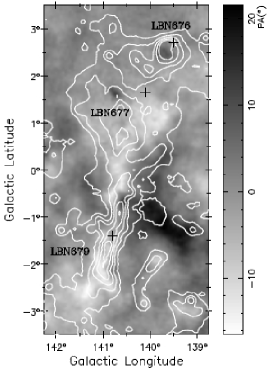
Figure 9: $PA$ distribution in B-field direction for the “drumstick” area. $I$ contours start at 1.5 mK $\rm T_{B}$ and run in steps of 12 mK $\rm T_{B}$. Crosses show the central positions of the optically visible H II regions.

LBN 676 and LBN 679 are supposed to be at the same distance in the Perseus arm. They were already investigated in some detail by Green (1989) using DRAO Synthesis Telescope data at 408 MHz and discussed together with infrared and HI maps. Green (1989) found that the elongated H II region LBN 679 coincides with a large H I spur located in the Perseus arm and pointed out that it is a thermal rather than a non-thermal feature as suggested by Kallas (1983).

Karr & Martin (2003) studied all three H II regions with 1$\arcmin$ resolution using CGPS data at 1.4 GHz (Taylor et al. 2003). The thermal character of LBN 679 was again confirmed and in addition they derived a thermal spectrum with $\beta=-1.85\pm 0.1$ for LBN 676, thus excluding a possible SNR identification considered by Green (1989) for this shell structure. The $\lambda$6 cm data agree with the thermal properties of all objects through a check of their temperature spectral indices via TT-plots using Effelsberg $\lambda$21 cm data for comparison.

All three LBNe appear to be depolarized at $\lambda$6 cm when large-scale polarized emission is added. Estimates of the magnetic field strength from modeled $RM_{FS}$ require the thermal radio continuum brightness temperature to find their $EM$. For a known distance the source size and $n_{e}$ need to be calculated in addition. Green (1989) assumed that LBN 676 and LBN 679 are both at a distance of 3 kpc in the Perseus arm. However, the Perseus arm distance was revised by Xu et al. (2006) to be about 2 kpc by triangulation of W3OH, which is just about 7$\degr$ apart in Galactic longitude. In the following we adopt this distance.

It turns out that a ring average of the PA/PI differences for LBN 676 is difficult to perform because of confusion with LBN 677 emission. Thus we just take the data from the upper part. The model fit gives the best result (Fig. 10) for the first five pixels as $RM_{FS}=280\pm$30 rad m^-2. Foreground polarized emission comprises about 79% while $\mathit{f}=0.80$. Likely most of the polarized emission originates in the local arm. The total intensity attributed to LBN 676 is about 50 mK $\rm T_{B}$ at $\lambda$6 cm. An apparent diameter of $0\aas@@fstack{\circ}8$ equals to a path length of 28 pc for 2 kpc distance. We obtain $n_{e}$ as about 3.3 cm^-3 and $B_{\parallel}$ $\approx$ +3.7 $\mu$G.

In the southern part of the 2$\degr$ long filamentary LBN 679, we find large $PA$ changes and also in its outskirts beyond. There is an inclined elongated $PA$ structure, about 1$\degr$ long, running from northeast to southwest. Model fitting (Fig. 11) is done for a 35$\degr$ wide cone in south-western direction of the rim. Best fit for the first ten pixels gives $RM_{FS}=-155\pm$15 rad m^-2, a foreground polarization fraction of about 60% for $\mathit{f}=0.85$. From the $\lambda$6 cm brightness temperature of about 40 mK $\rm T_{B}$ and assuming a line-of-sight length of the source of 35 pc, we calculated $B_{\parallel}$ = $-2.0\leavevmode\nobreak\ \mu$G and $n_{e}$ = 2.7 cm^-3. To the lower left direction of LBN 679, another $PA$ structure is located at about $\ell=141\aas@@fstack{\circ}35,b=-2\aas@@fstack{\circ}60$.

Figure 10: Average values in northern direction for the H II region LBN 676. Offsets are relative to the centre coordinate ($\ell=139\aas@@fstack{\circ}65,b=2\aas@@fstack{\circ}45$). $PA$ difference and $PI$ ratio are shown in the upper and middle panel, respectively. The vertical dashed line indicates the boundary between the “$\mathrm{on}$” and “$\mathrm{off}$” components.

Figure 11: Average values starting from the coordinate ($\ell=141\aas@@fstack{\circ}10,b=-2\aas@@fstack{\circ}00$) to the outskirts of the H II region LBN 679 in a sector from 10$\degr$ to 45$\degr$ counting from south (0$\degr$) to west .

Karr & Martin (2003) found that the northern part of LBN 677 is associated with the exciting star HD 19820 at 1 kpc distance. 0.8 kpc distance were quoted for associated CO-emission (Blitz et al. 1982), which we adopt in the following discussion. A circular average is difficult to apply to the large area of LBN 677 due to significant variations and the non-symmetric distribution of $PA$. Different signs of $PA$ in different areas indicate changing properties throughout the entire region. We select the western part of LBN 677, where $PA$ changes smoothly for modeling. Based on the central five pixels average, the best fit (Fig. 12) gives a $RM_{FS}$ value of $-150\pm$40 rad m^-2. 69% of the total polarized emission originates in the foreground. The depolarization factor is $\mathit{f}$ = 0.88. The 2$\degr$ diameter source gives a depth of 28 pc assuming a spherical shape. With the $\lambda$6 cm brightness temperature of about 20 mK $\rm T_{B}$ we calculate $EM$ = 137 pc cm^-6. $B_{\parallel}$ then is $-3.0\leavevmode\nobreak\ \mu$G and $n_{e}$ about 2.2 cm^-3. The reddening measurement of the exciting star HD 19820 ($\ell=140\aas@@fstack{\circ}12,b=1\aas@@fstack{\circ}54$) is about 0.82 (Hiltner 1956). The H$\alpha$ intensity is about 14 Rayleigh (Finkbeiner 2003) after subtracting a background level of 11 Rayleigh. We obtain $EM$ as 233 pc cm^-6 by Eq. 3. Then $B_{\parallel}$ reduces to $-2.3\leavevmode\nobreak\ \mu$G and $n_{e}$ increases to 2.9 cm^-3. The physical parameters from both methods are similar. The best fit of $PI_{fg}$ for LBN 676 and LBN 679 is around 70%. We found almost the same value also for LBN 677, which is unexpected in view of their different distances. If the polarized emissivity in this direction is fairly constant, this may indicate that LBN 677 is also at about 2 kpc distance. For this distance $B_{\parallel}$ will change to $-1.9\leavevmode\nobreak\ \mu$G and $n_{e}$ to 1.4 cm^-3.

We summarize the derived parameters for the three LBNe in Table 3. We note that our modeled $B_{\parallel}$ are rather similar to those found for H II regions with a similar low electron density, e.g. S264 (Heiles et al. 1981) and G124.9+0.1 (Paper I).

Table 3: Physical parameters for three LBNe

H II region	LBN 676	LBN 677	LBN 679
$EM$(pc cm-6)	305	137 (233)	255
$n_{e}$(cm-3)	3.3	1.4a/2.2b (2.9b)	2.7
$RM_{FS}$(rad m-2)	280	-150	-155
$B_{\parallel}$($\mu$G)	3.7	-1.9a/-3.0b (-2.3b)	-2.0
a is derived for a distance of 2 kpc;
b is derived for a distance of 800 pc.

For LBN 677 we use the two $EM$ values derived from radio
emission and H$\alpha$ emission (see Sect. 3.4.3).

Figure 12: Half ring average values from centre coordinate ($\ell=139\aas@@fstack{\circ}70,b=1\aas@@fstack{\circ}10$) towards the west of LBN 677.

Besides the three LBN objects there are more $\lambda$6 cm Faraday Screen structures in the field of Fig. 9. Some were listed below, which we, however, will not analyze in detail in this paper. A large area with very uniform $PA$s, which deviate about 22$\degr$ from the Galactic plane direction, can be identified in southwestern direction of the “drumstick”. This Faraday Screen is centered at around $\ell=139\aas@@fstack{\circ}70,b=-1\aas@@fstack{\circ}20$. There is no counterpart in the $I$ map (see Fig. 9), thus the thermal electron density must be very low. Polarization observations at other wavelengths are needed to analyze this feature in some detail. Also the small objects at $\ell=139\aas@@fstack{\circ}95,b=-2\aas@@fstack{\circ}05$ and at $\ell=139\aas@@fstack{\circ}20,b=-3\aas@@fstack{\circ}00$ were found to be thermal (Gao et al., in prep.) and act as Faraday Screens. They also can be clearly identified in the $PA$ map (Fig. 9).

3.4.4 G146.4-3.0

G146.4-3.0 is a large Faraday Screen with a diameter of approximately $3\aas@@fstack{\circ}3$, centered at $\ell=146\aas@@fstack{\circ}40,b=-3\aas@@fstack{\circ}00$. This structure shows highly polarized emission in the original $PI$ map at $\lambda$6 cm and becomes depolarized after large-scale polarized emission is added. No counterpart can be found in the $I$ map (see Fig. 13). The H$\alpha$ intensity in this region is in general low and does not show any excess related to this Faraday Screen.

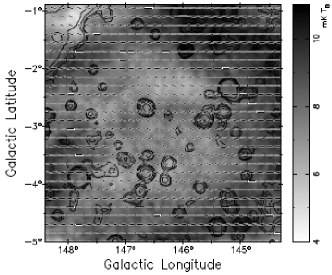
Figure 13: $PI$ of the Faraday Screen G146.4-3.0 in grey scale. $I$ contours are overlaid running from $3\sigma$, or 1.5 mK $\rm T_{B}$, in steps of 2${}^{n-1}\ \times$ 1.0 mK $\rm T_{B}$. Bars show B-vectors for every third pixel ($9\arcmin$) in $\ell$ and $b$ direction.

A Faraday Screen model fit (Fig. 14) results in an average $RM_{FS}$ for the central area of 1$\degr$ diameter of $-140\pm$20 rad m^-2. 26% of total $PI$ in this area originates in front of the Faraday Screen for $\mathit{f}$ = 0.97. The $RM$ value is not exceptionally high, but the scatter across the Faraday Screen is large enough to make the object invisible in the $\lambda$21 cm polarization survey by Landecker et al. (2010, submitted), although their survey only covers the northern area of the Faraday Screen.

Figure 14: Ring averaged data and modeled $RM$s for Faraday Screen G146.4-3.0 shown in Fig. 13.

The distance to this prominent Faraday Screen in the $\lambda$6 cm survey is not clear. To derive $n_{e}$ by its free-free $EM$ we used the 3$\sigma$ level of the $\lambda$6 cm $I$ map, means about 1.5 mK $\rm T_{B}$, as a brightness temperature upper limit. The fitted central $B_{\parallel}$ and $n_{e}$ are estimated and shown in Fig. 15 as a function of distance. Note that $n_{e}$ is always an upper limit, while $B_{\parallel}$ has to be taken as minimum.

The foreground polarized emission of about 26% is small compared to the fraction of about 70% obtained for the LBNe in the Perseus arm (see Sect. 3.4.3). Thus the distance to G146.4-3.0 should be small. Assuming the polarized emissivity along the line of sight to be the same as to the Perseus LBNe of about 3.4 mK kpc^-1, we estimate the distance to Faraday Screen G146.4-3.0 as about 690 pc, which implies a diameter of the Faraday Screen of about 40 pc. Then $B_{\parallel}$ for its central area is about $-8.6\leavevmode\nobreak\ \mu$G and $n_{e}$ is about 0.5 cm^-3. However, the local emissivity is known to be two to three times larger than the average emissivity at 2 kpc distance (Fleishman & Tokarev 1995). This will reduce the distance and the size of the Faraday Screen accordingly. For a distance of 280 pc, its size reduces to about 16 pc, $n_{e}$ increases to about 0.8 cm^-3 and $B_{\parallel}$ to $-13.5\leavevmode\nobreak\ \mu$G.

Taylor et al. (2009) re-analyzed the NVSS (Condon et al. 1998) polarization data. $RM$s for 37 543 polarized radio sources were derived. We examine our Faraday Screen model result by checking the $RM$s in the area of Fig. 13. Two sources are located within the area of the Faraday Screen. The $RM$s of the two sources $\ell=146\aas@@fstack{\circ}62,b=-2\aas@@fstack{\circ}69$ and $\ell=146\aas@@fstack{\circ}63,b=-3\aas@@fstack{\circ}81$ are $-151.1\pm$8.2 rad m^-2 and $-221.9\pm$8.4 rad m^-2, respectively. For another source at $\ell=145\aas@@fstack{\circ}61,b=-2\aas@@fstack{\circ}9$ Brown et al. (2003a) reported a $RM$ value of $-338\pm$15 rad m^-2 from the CGPS, which is the most excessive $RM$ value. Outside the Faraday Screen area Taylor et al. (2009) list $RM$s for 15 sources with an average $RM=-75.7\pm$30.4 rad m^-2. Despite significant scatter the three sources show excessive negative $RM$s, which seem to be attributed to G146.4-3.0.

Figure 15: Dependence of the central $B_{\parallel}$ and $n_{e}$ from the distance to the Faraday Screen G146.4-3.0.

3.4.5 Large magnetic bubbles at $\ell=165\degr$

Two coinciding magnetic bubbles of different sizes were identified in the area $\ell$ around $165\degr$ by Kothes & Landecker (2004) from polarization observations with about 1$\arcmin$ resolution at $\lambda$21 cm with the DRAO synthesis telescope. These bubbles were also seen in the Effelsberg 1.4 GHz polarization data (Reich et al. 2004) at 9$\aas@@fstack{\prime}4$ resolution. The smaller bubble extends from $\ell$ = 164$\degr$ to $167\aas@@fstack{\circ}5$ and $-2\degr$ to 2$\degr$ in $b$, while the larger one has about the same projected centre but is approximately 9$\degr$ in size. At $\lambda$6 cm the two bubbles become very faint. The $\lambda$21 cm map (Kothes & Landecker 2004) was limited to $b=-3\degr$, while the $\lambda$6 cm map shows the larger bubble to extend approximately to $b=-5\degr$ (Figs. 4 and 16).

The bubbles are faint but visible in the $\lambda$6 cm Stokes $U$ map (Fig. 16). They are marginally traced in the Stokes $Q$ map, regardless of including large-scale polarized emission or not. At $\lambda$6 cm the bubbles can not be identified as discrete objects in $PI$ exceeding just a few times the rms-noise value of about 0.4 mK $\rm T_{B}$, although some individual patches or filaments with stronger emission in this large area may be attributed to them. The faintness of the bubbles indicates that either their $RM$ is not as high as that of the more pronounced $\lambda$6 cm Faraday Screens described in this paper, or that the polarized background emission is very faint in respect to the foreground, e.g. in terms of our Faraday Screen model $c$ is close to 1.

In their preliminary model Kothes & Landecker (2004) discussed the large bubble as a Faraday Screen with a rather low electron density in agreement with the low H$\alpha$ emission in its direction. Rather important is the association of an H I bubble identified in the CGPS data with a velocity of about $-20$ km s^-1 surrounding the outer larger magnetic bubble, which makes it a Perseus arm object at 1.5 kpc to 2 kpc distance. This results in a very large object of about 240 pc to 310 pc in diameter. Our $\lambda$6 cm data will not improve the physical parameters of the bubbles.

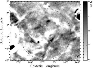
Figure 16: $U$ map at $\lambda$6 cm of the large magnetic bubble. The dotted line outlines the outer boundary of the bubble as quoted by Kothes & Landecker (2004).

3.4.6 The $\ell=173\degr$ H II complex

The survey region around $\ell=173\degr$ is very rich in structures (Fig. 17). Nine H II regions from the Sharpless catalogue are located within this very extended “bow-tie” shaped complex with the most prominent and extended H II region, SH 2-236, located in the southeast. There are four H II regions, SH 2-231, SH 2-232, SH 2-233 and SH 2-235 located in the north, among which, SH 2-235 is the strongest. The so-called “Spider Nebula” and the “Fly Nebula”, SH 2-234 and SH 2-237, are seen in the middle of the complex, while SH 2-229 is located in the south-west. The central diffuse emission is attributed to SH 2-230. All these H II regions are infrared-bright sources. Besides the Sharpless H II regions additional ridge-shaped structures are seen in the $\lambda$6 cm $I$ map, for example at $\ell=171\aas@@fstack{\circ}20,b=2\aas@@fstack{\circ}35$ and $\ell=172\aas@@fstack{\circ}65,b=3\aas@@fstack{\circ}60$. Thermal characteristics of these filamentary structures are confirmed by applying the TT-plot method to derive spectral information between the $\lambda$6 cm and the corresponding Effelsberg $\lambda$21 cm survey map.

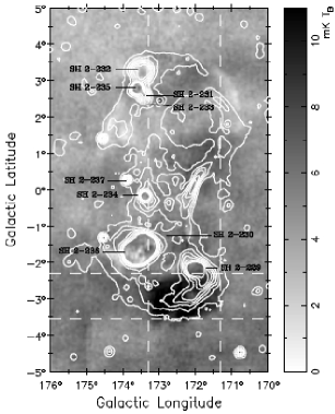
Figure 17: $\ell$=173$\degr$ H II complex. Restored $PI$ in grey scale overlaid by $I$ contours are shown. The contour lines run from 7 mK $\rm T_{B}$ in steps of 15 mK $\rm T_{B}$ up to 112 mK $\rm T_{B}$. The two large rectangular regions (vertical and horizontal) marked by dashed lines are the regions where $I$, $PA$ and $PI$ were averaged as shown in Fig. 18.

Excessive polarized emission extending for about $2\aas@@fstack{\circ}0\times 1\aas@@fstack{\circ}3$ is seen in the southern part of the complex, distinct from SH 2-229 and SH 2-236 (Fig. 17). $PI$ is about 3 mK $\rm T_{B}$ higher compared to its surroundings (Fig. 18). The distances to the two Sharpless regions are 510 pc for SH 2-229 and 3.2 kpc for SH 2-236 (Blitz et al. 1982). No morphological resemblance exists between the polarized patch and total intensity emission, while it seems that the western part of the polarized structure is overlapped with a southern extension from SH 2-229 (see Fig. 17). This patch coincides with thermal absorption structures visible in the low-frequency maps at 10 MHz by Caswell (1976) and at 22 MHz by Roger et al. (1999) as shown in Fig. 19. Thus we expect thermal emission to act as a Faraday Screen. However, we can not apply our simple Faraday Screen model, because the polarized “$\mathrm{on}$” emission exceeds the “$\mathrm{off}$” emission, which requires that the background and the foreground $PA$s are different. According to the starlight polarization catalogue by Heiles (2000), large $PA$ variations are observed in this direction. High-angular resolution Galactic emission simulations as described by Sun & Reich (2009) were used to simulate the $\lambda$6 cm $PA$, $PI$ and $I$ as a function of distance (Fig. 20). A significant change of $PA$ is seen for distances below 300 pc, which is needed to explain a $PI$ excess by Faraday rotation. This indicates that the Faraday Screen is nearer than 300 pc.

Figure 18: Upper plot shows $I$, $PA$ and $PI$ averaged in the vertical rectangle region marked in Fig. 17, where data are averaged in columns. The vertical dashed lines mark the boundary of the highly polarized emission region. The lower plot shows the results when averaging in the horizontal rectangle in Fig. 17.

Low-frequency absorption is more pronounced by local features with strong emission background than by more distant objects having the same physical properties. The clear absorption at 10 MHz and 22 MHz of G172.3-2.9 (see Fig. 19) further supports a local origin. The recent 1.4 GHz polarization survey by Landecker et al. (2010, submitted) with 1$\arcmin$ angular resolution does not show a corresponding $PI$ structure, however, the $PA$ distribution is rather smooth in this area. Observations at other wavelengths are needed to constrain the properties of this outstanding Faraday Screen in our $\lambda$6 cm map.

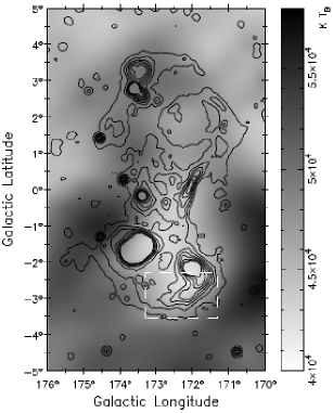
Figure 19: 22 MHz $I$ map in grey scale of the $\ell$=173$\degr$ H II complex overlaid by $\lambda$6 cm $I$ contours. The contour intervals are the same as in Fig. 17. Strong thermal absorption can be seen in the region with excessive $PI$ at $\lambda$6 cm.

Figure 20: Simulated and accumulated $\lambda$6 cm $PA$, $PI$ and $I$ data as a function of distance in the direction $\ell=172\aas@@fstack{\circ}3,b=-2\aas@@fstack{\circ}9$. The data are averaged within $0\aas@@fstack{\circ}2$.

4 Summary

In Paper II, we present the second section covering the outer Galaxy for the area $129\degr\leq\ell\leq 230\degr$, $|b|\leq 5\degr$ of the Sino-German $\lambda$6 cm polarization survey of the Galactic plane at an angular resolution of $9\aas@@fstack{\prime}5$. It is the ground-based polarization survey at the highest frequency for the Galactic anti-centre region. The observed polarization data have been restored to an absolute level by adding extrapolated large-scale components from the WMAP K-band polarization maps (Hinshaw et al. 2009).

Numerous newly detected Faraday Screens indicate the presence of large magnetic bubbles in the ISM hosting regular magnetic fields of a few $\mu$G. A simple model fit to selected Faraday Screens, which also includes H II regions, was used to estimate their physical parameters. Our main results are:

1. We note that the remarkable polarized “lens” Faraday Screen in front of W5 detected by Gray et al. (1998) at $\lambda$21 cm becomes invisible at $\lambda$6  cm, while previously unknown polarized structures were detected at $\lambda$6 cm at the boundaries of W5.

2. The Faraday Screen model fits for LBN 676, LBN 677 and LBN 679 indicate that besides the established Perseus arm objects LBN 676 and LBN 679 also LBN 677 is located in the Perseus arm rather than at 0.8 kpc distance, because its polarized foreground level is as that of the other two objects. The parameters of the three LBNe are listed in Table 3. For LBN 676 the model fit indicates a magnetic field direction opposite to those of the other two LBNe. A similar case was noted by Mitra et al. (2003) for a few Perseus arm H II regions based on pulsar $RM$s shining through them.

3. The newly discovered extended Faraday Screen G146.4-3.0 is likely quite local. $B_{\parallel}$ is estimated to be about $-8.6\leavevmode\nobreak\ \mu$G if located at 690 pc, which is most likely an upper limit. The field strength within G146.4-3.0 will increase in case its distance is smaller.

4. The two huge polarized bubbles located at $\ell=165\degr$ as revealed by Kothes & Landecker (2004) at $\lambda$21 cm become very faint at $\lambda$6 cm.

5. An extended blob showing excessive polarized emission is detected in the lower area of the “bow-tie” shaped H II region complex around $\ell=173\degr$. Absorption at lower radio frequencies coincides with the $PI$ excess. We find evidence that this is a local Faraday Screen with a likely distance smaller than 300 pc.

For most of the selected Faraday Screens the polarized emission becomes weaker compared to their surroundings. This is expected when the $PA$ of the background polarization is rotated away from the foreground direction. The polarized emission exceeds that of the surroundings only in case the difference of the $PA$s is reduced.

The selected Faraday Screens from the $\lambda$6 cm polarization survey demonstrate the existence of numerous high-$RM$ features in the interstellar medium. These structures cover a significant fraction of the surveyed area. $RM$ studies based on pulsars or extragalactic sources aiming to derive the parameters of the large-scale Galactic magnetic field need to take the $RM$-contribution from Faraday Screens into account. The formation of strong regular magnetic fields in thermal low-density regions exceeding the interstellar value needs to be investigated. We note that most of the Faraday Screens visible at $\lambda$6 cm are not seen at longer wavelengths, where their $RM$ causes polarization angle rotations exceeding $180\degr$. Missing depolarization implies that small-scale fluctuations across the beam may not be significant.