Turnstile pumping through an open quantum wire

Abstract

We use a non-Markovian generalized master equation (GME) to describe the time-dependent charge transfer through a parabolically confined quantum wire of a finite length coupled to semi-infinite quasi two-dimensional leads. The quantum wire and the leads are in a perpendicular external magnetic field. The contacts to the left and right leads depend on time and are kept out of phase to model a quantum turnstile of finite size. The effects of the driving period of the turnstile, the external magnetic field, the character of the contacts, and the chemical potential bias on the effectiveness of the charge transfer of the turnstile are examined, both in the absence and in the presence of the magnetic field. The interplay between the strength of the coupling and the strength of the magnetic field is also discussed. We observe how the edge states created in the presence of the magnetic field contribute to the pumped charge.

I Introduction

The time-dependent properties of semiconductor nanostructures and their response to electric pulses are currently being studied through transient current measurements and in a pump-and-probe configuration.Tarucha ; Lai ; Naser Along with these experimental developments theoretical schemes for the description of time-dependent transport emerged. The methods include the non-equilibrium Keldysh-Green function formalism,Stefanucci ; Moldo scattering theory, Gudmundsson and more recently the generalized master equation (GME) adapted for electronic transport.Harbola ; NJP1 ; Welack1

These methods were used mostly for studying the transient currents generated by a time-dependent potential applied on the sample or by a time-dependent coupling between the leads and the sample. An example in the first category is the time dependent pumping of electrons through a small open system.Stefanucci In the second category we mention the transient currents and the geometrical effects imposed by the lateral confinement of the sample.NJP1 ; NJP2 In another recent work we investigated the modulation of the drain current when a sequence of square pulses is applied to the source probe connected to a quantum dot and a short quantum wire described within lattice model.PRB1 That study was motivated by the experiments of Naser et al.Naser

In the present work we further exploit the GME method and study the transport properties of a quantum wire operating in a turnstile regime. The turnstile pump is a single-electron device where the sample is periodically connected and disconnected with the left and right lead respectively, but with a relative phase shift. It was experimentally created by Kouwenhoven et al.TSP by modulating in time the two tunneling barriers between a quantum dot and two leads. The electrons were driven by a finite bias between the leads. This setup is different from a quantum pump where a current is generated by asymmetric external oscillations, but without a bias. In the experiment of Kouwenhoven et al. the barrier heights oscillate out of phase in the following sense: On the first half-cycle electrons enter from the source probe in the system but there is no current in the drain probe because the corresponding tunneling barrier is high enough to prevent this. In the second half-cycle the source is disconnected, the drain contact opens, and a discharge of the dot follows. It was found that an integer number of electrons are transmitted through the structure in each pumping cycle.

More recently, due to the general interest in applications of nanoelectronic devices, more complex turnstile pumps have been studied by numerical simulations, like one-dimensional arrays of junctions Mizugaki or two-dimensional multidot systems. Ikeda In the present paper we predict that the turnstile operation can also be performed in a quantum wire sample and in an external magnetic field as well. Our results are obtained using a parabolic lateral confinement model both for the quantum wire and for the leads. We put a special effort on describing the lead-sample contacts. In a previous work we studied the turnstile transport through a sample described by a lattice (tight-binding) model. The sample was a one-dimensional system with two or three sites and the transport calculations were done using nonequilibrium Keldysh-Green functions.TSPPRB The quantum wire considered in this work is much more complex. We start from the single-particle Hamiltonian of a two-dimensional wire of length $L_{x}$ parabolically confined along the $y$ direction and with hard-wall conditions at $\pm L_{x}/2$. The eigenfunctions of the Hamiltonian were described in detail in Ref. Gudmundsson, and will not be repeated here.

The material is organized as follows: In Section II we briefly review the main equations of the model and of the GME method, Section III is devoted to the numerical results for zero magnetic field (III.1), in the presence of a magnetic field (III.2), and to the edge states (III.3). The conclusion are given in Section IV.

II The model

We consider an isolated finite quantum wire of length $L_{x}=300$ nm, extended in the $x$-direction. The width of the wire is defined by a parabolic confinement potential in the $y$-direction with the characteristic energy $\hbar\Omega_{0}=1.0$ meV. The quantum wire is terminated at $\pm L_{x}/2$ with hard wall potentials. In addition, we have two semi-infinite leads, one extended from $-L_{x}/2$ to $-\infty$, and the other one from $+L_{x}/2$ to $+\infty$. Both have a parabolic confinement in the $y$ direction with an energy of 0.8 meV, and are also terminated at $\pm L_{x}/2$ with hard walls. The leads and the finite quantum wire, or the system, are all subjected to an external constant magnetic field $\mathbf{B}=B\mathbf{\hat{z}}$. The length of the wire, $L_{x}$, and the magnetic length modified by the parabolic confinement $a_{w}=\sqrt{\hbar/(m^{*}\Omega_{w})}$, with $\Omega_{w}^{2}=\Omega_{0}^{2}+\omega_{c}^{2}$ and the cyclotron frequency $\omega_{c}=eB/(m^{*}c)$, are convenient length scales in the calculations. We assume the GaAs effective mass, $m^{*}=0.067m_{e}$. The many-electron Hamiltonian of the system composed by the semi-infinite leads and the finite quantum wire, but isolated from each other, is:

$$H(t)=\sum_{a}E_{a}d^{\dagger}_{a}d_{a}+\sum_{q,l=\mathrm{L,R}}\epsilon_{l}(q)c^{\dagger}_{ql}c_{ql},$$ (1)

where an electron in the system is created (annihilated) by the operators $d^{\dagger}$ ($d$), and in the leads by $c^{\dagger}$ ($c$). $E_{a}$ are the energies of the single-electron states labeled with $a=1,2,3,...$ in increasing order, $\epsilon_{l}(q)$ is the energy spectrum of the left and right leads, labeled as $l=\mathrm{L}$ and $l=\mathrm{R}$ respectively, and $q$ representing a discrete label of subbands and a continuous quantum number labeling states within each subband. At $t=0$ the system is coupled to the leads with the Hamiltonian

$$H_{\mathrm{T}}(t)=\sum_{l}\chi_{l}(t)\sum_{q,a}\left\{T^{l}_{qa}c_{ql}^{\dagger}d_{a}+(T^{l}_{qa})^{*}d_{a}^{\dagger}c_{ql}\right\},$$ (2)

with $\chi_{l}(t)$ describing the time-dependence of the coupling, such that $\chi_{l}(t<0)=0$, and $T^{l}_{qa}$ describing the coupling strength of state $a$ and $q$ in the system and the leads, respectively.

The coupling is defined by a nonlocal overlap integral of the two states in the region of contact around $\pm L_{x}/2$. The coupling coefficients are defined phenomenologically with the tensor NJP2

$$T^{l}_{aq}=\int_{\Omega_{S}^{l}\times\Omega_{l}}d{\bf r}d{\bf r}^{\prime}\left(\Psi^{l}_{q}({\bf r}^{\prime})\right)^{*}\Psi^{S}_{a}({\bf r})g^{l}_{aq}({\bf r},{\bf r^{\prime}})+h.c.,$$ (3)

where a nonlocal-overlap of the wave functions in the system and the leads is modeled by

$$g^{l}_{aq}({\bf r},{\bf r^{\prime}})=g_{0}^{l} \exp{\left[-\delta_{1}^{l}(x-x^{\prime})^{2}-\delta_{2}^{l}(y-y^{\prime})^{2}\right]}$$

$$\exp{\left(\frac{-|E_{a}-\epsilon^{l}(q)|}{\Delta_{E}^{l}}\right)}.$$ (4)

The strength of the coupling between the leads and the sample is defined by the parameter $g_{0}^{l}$, which captures the tunneling rate at the contact between each lead and the sample, and also by the parameters $\delta_{1}^{l}$, $\delta_{2}^{l}$ and $\Delta_{E}^{l}$ which adjust the spatial overlap of lead and sample wave functions in the contact region. Since all we have from our model are the wave functions derived for the uncoupled subsystems, this intuitive ansatz, Eqs. (3) and (4), is a convenient way of describing the coupling. In our calculations these coupling parameters will be the same for both leads and hence the label $l$ will be omitted.

The system can be subjected to a bias $\Delta\mu=\mu_{L}-\mu_{R}$ and in order to reduce the number of many-electron states (MES) to a reasonable number in the following calculations we limit the number of single-electron states (SES) for the particular calculation by selecting a window of relevant states around the bias window, i.e. $[\mu_{R}-\Delta,\mu_{L}+\Delta]$, such that the transport properties are not changed significantly by extending the window. We consider these states relevant for the transport, or “active”, while all the other states are “frozen”, being either permanently occupied or permanently empty. In addition to the electrons frozen in the states below the active window (which are not included in the transport calculation), we also assume the lowest active state occupied at the moment $t=0$ i. e. when the contacts begin to operate. In this way the transient phase is shorter than if we would assume an empty active window, and we can spend less computing time until the system reaches the periodic state.

The time-evolution of the total system - finite wire and leads - after the coupling at $t=0$, can be described by the Liouville-von Neumann equation for the statistical operator $W(t)$. The evolution of the finite wire itself can be captured by the reduced density operator $\rho(t)=\mathrm{Tr_{L}Tr_{R}}W(t)$ (RDO), i. e. by averaging over the the lead variables. From the resulting integro-differential equation we retain only the lowest order (quadratic) terms in $H_{T}$ and obtain NJP1 ; NJP2

$${\dot{\rho}}(t)= - \frac{i}{\hbar}[H_{\mathrm{S}},\rho(t)]$$ (5)

$$- \frac{1}{\hbar^{2}}\sum_{l=\mathrm{L,R}}\int dq\>\chi_{l}(t)([{\cal T}_{l},\Omega_{ql}(t)]+h.c.),$$

where we have introduced two operators to compactify the notation

$$\Omega_{ql}(t)=U_{\mathrm{S}}^{\dagger}(t)\int_{t_{0}}^{t}ds\>\chi_{l}(s)\Pi_{ql}(s)e^{i((s-t)/\hbar)\varepsilon_{l}(q)}U_{\mathrm{S}}(t),$$

$$\Pi_{ql}(s)=U_{\mathrm{S}}(s)\left({\cal T}_{l}^{\dagger}\rho(s)(1-f_{l})-\rho(s){\cal T}_{l}^{\dagger}f_{l}\right)U_{\mathrm{S}}^{\dagger}(t),$$

with $U_{\mathrm{S}}(t)=e^{i(t/\hbar)H_{\mathrm{S}}}$, and a scattering operator ${\cal T}$ acting in the many-electron Fock space of the system

$${\cal T}_{l}(q) = \sum_{\alpha,\beta}{\cal T}_{\alpha\beta}^{l}(q)|{\bf\alpha}\rangle\langle{\bf\beta}|\ ,$$

$${(\cal T}_{l}(q))_{\alpha\beta} = \sum_{a}T^{l}_{aq}\langle{\bf\alpha}|d_{a}^{\dagger}|{\bf\beta}\rangle\ .$$ (6)

With the RDO it is possible to calculate the statistical average of the charge operator $Q_{\mathrm{S}}=e\sum_{a}d_{a}^{\dagger}d_{a}$ for the coupled system

$$\langle Q_{\mathrm{S}}(t)\rangle = {\rm Tr}\{W(t)Q_{\mathrm{S}}\}={\rm Tr}_{\mathrm{S}}\{[{\rm Tr}_{\mathrm{LR}}W(t)]Q_{\mathrm{S}}\}$$ (7)

$$= {\rm Tr}_{\mathrm{S}}\{\rho(t)Q_{\mathrm{S}}\}=e\sum_{a,\mu}i^{\mu}_{a}\,\langle\mu|\rho(t)|\mu\rangle,$$

with the traces assumed over the Fock space. The average time-dependent spatial distribution of the charge can also be obtained,

$$\langle Q_{\mathrm{S}}({\bf r},t)\rangle=e\sum_{ab}\sum_{\mu\nu}\Psi^{*}_{a}({\bf r})\Psi_{b}({\bf r})\rho_{\mu\nu}(t)\langle\nu|d^{\dagger}_{a}d_{b}|\mu\rangle.$$ (8)

The net current flowing into the sample is

$$\langle J(t)\rangle = \langle J_{\mathrm{L}}(t)\rangle-\langle J_{\mathrm{R}}(t)\rangle$$

$$= \frac{d\langle Q_{\mathrm{S}}(t)\rangle}{dt}=e\sum_{a}\sum_{\mu}i^{\mu}_{a}\,\langle\mu|\dot{\rho}(t)|\mu\rangle\,.$$

The total current in Eq. (II) is given by the left hand side of the GME, Eq. (5), and the partial currents associated to each SES and each lead correspond to the terms of the sum on the right hand side (the trace of the commutator of $\rho$ and $H_{\mathrm{S}}$ is zero).

The functions which modulate the coupling between the leads and the quantum wire are built in the following way: For $0\leq t<T_{l}$ we use the Fermi-like function $f(t)=(e^{t\gamma}+1)^{-1}$, with $\gamma=1.0$ ps^-1, and we define $\chi_{l}(t)=1-2f(t)$, where $l=\mathrm{L,R}$ is the lead index. Then, for $t\geq T_{l}$, $\chi_{l}(t)$ become step-like functions alternating between 0 and 1, both with the same period $T$, but with a delay of $T/2$. In this way we mimic the on/off contact switching done in the turnstile experiments. We choose $T_{\mathrm{L}}<T_{\mathrm{R}}=T_{\mathrm{L}}+T/2$, which means we first switch off the left contact while the right one is still on. Then the left is turned on again while the right is turned off, and so on.

III Numerical calculations, results, and discussion

III.1 No magnetic field

The energy spectrum of the leads and of the sample are shown in Fig. 1. The leads have parabolic subbands while the sample has discrete levels. The maximum energy for each subband shown in the graph indicates the corresponding maximum wave vector in the $qa_{w}$-integration of the GME. The chemical potentials in the leads defining the bias window (BW) are shown with the dashed horizontal lines. We consider two BW’s: BW1 with chemical potentials $\mu_{L}=1.48$ meV and $\mu_{R}=0.78$ meV, and BW2 with $\mu_{L}=2.48$ meV and $\mu_{R}=1.78$ meV respectively. In both cases the applied bias is $eV_{\mathrm{bias}}=\mu_{L}-\mu_{R}=0.70$ meV. In the numerical calculations of the reduced statistical operator we also include the sample states with energy outside the BW, between the limits $\mu_{R}-\Delta$ and $\mu_{L}+\Delta$ with $\Delta=0.1$ meV. The first active window contains 4 SESs and the second one contains 5 SESs.

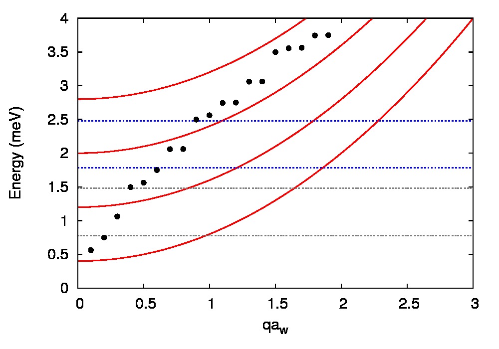
Figure 1: (Color online) The energy spectrum of the leads vs. the scaled wave vector $qa_{w}$. The subband index is $n=0,1,2,3$. With dots the energy spectrum of the isolated sample. With horizontal wide dashed lines the chemical potentials $\mu_{L}=1.48$ meV and $\mu_{R}=0.78$ (BW1), and with horizontal narrow dashed lines $\mu_{L}=2.48$ meV and $\mu_{R}=1.78$ meV (BW2).

In Fig. 2 we show the time-dependent total occupation $n_{t}$ of the relevant (active) SES for BW1 and BW2. The electrons occupying the states situated below the active windows are not included, but only those on the relevant states (or within the active windows). In this example the parameters characterizing the coupling of the sample to the leads are $g_{0}a_{w}^{3/2}=926$ meV (with $a_{w}$ measured in nm), $\delta_{1}a_{w}^{2}=1.0$, and $\delta_{2}a_{w}^{2}=2.0$. The large value for $g_{0}a_{w}^{3/2}$ is consistent with the small overlap of the wave functions from the lead and from the sample mandated by the large values for $\delta_{1}a_{w}^{2}$ and $\delta_{2}a_{w}^{2}$. The largest contribution to the overlap comes from the “contact” area within one $a_{w}$ around the ends of the finite quantum wire at $x=\pm L_{x}$. The unusual dimension of $g_{0}$, which is $\mathrm{energy}\ \times\ \mathrm{length}^{-3/2}$ is a result of different dimensions of the wave functions in the lead and in the sample: the former is $\mathrm{length}^{-1/2}$, being unbounded in the direction along the lead, and the later is $\mathrm{length}^{-1}$. We also select $\Delta_{E}=0.25\hbar\Omega_{w}$ in Eq. (4). The time-dependent switching functions $\chi_{l}(t)$ are also shown in the figure, with period $T=60$ ps, for $l=\mathrm{L,R}$.

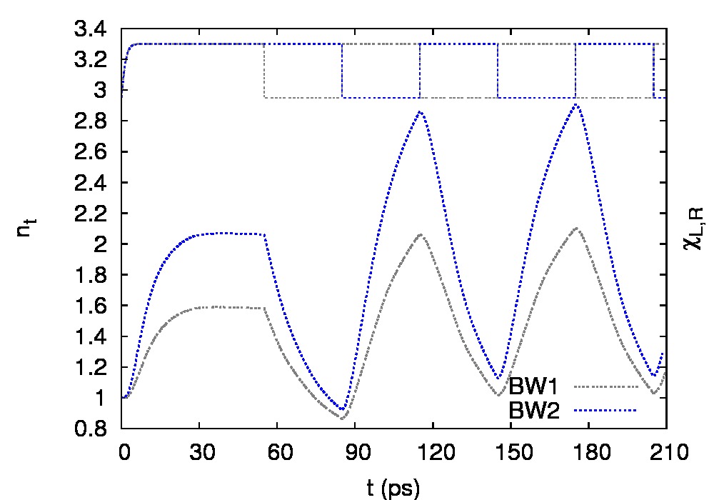
Figure 2: (Color online) The time dependent total occupation of the relevant SES for a system occupied initially with 1 electron ($\mu_{0}=2$) for the first (solid), and second (dotted) bias window. The time coupling functions $\chi_{l}(t)$, with $l=L,R$, are shown for reference. Other parameters: $g_{0}a_{w}^{3/2}=926$ meV, $\delta_{1}a_{w}^{2}=1.0$, $\delta_{2}a_{w}^{2}=2.0$, and $T=60$ ps. In each case there is one electron on the lowest relevant state at the initial moment.

Comparing the charge oscillation for the first and for the second active window we see that more charge is transferred through the system for BW2 than for BW1. There are two reasons for that. One reason is that BW2 includes three subbands of the leads, whereas BW1 includes only two (Fig. 1). The second reason is that the energy dispersion in each subband increases with increasing energy, such that the electrons have higher speed in BW2 than in BW1, and thus an increased contribution to conduction.

It is interesting to observe the behavior of the states situated at the boundaries of the BW. To show that we choose the BW1 and display in Fig. 3a the partial currents created by each sample state included in the calculation. These are the states 2,3,4,5 in the order of the energy, shown with dots in Fig. 1. State 1 (the lowest dot) is considered totally occupied and frozen. In this case state 2 is slightly below the window, state 3 is within the window, and states 4 and 5 are slightly above the window. In Fig. 3b we show the same partial currents, but now for a slightly higher chemical potential of the left lead, $\mu_{L}=1.54$ meV, instead of $\mu_{L}=1.48$ meV used in Fig. 3a. The state number 4 is now included in the BW and consequently the corresponding current increases. The current of the state 5 also increases a little bit, while the current associated to the other states does not change. A similar behavior is displayed by state number 9 situated on top of BW2 (not shown).

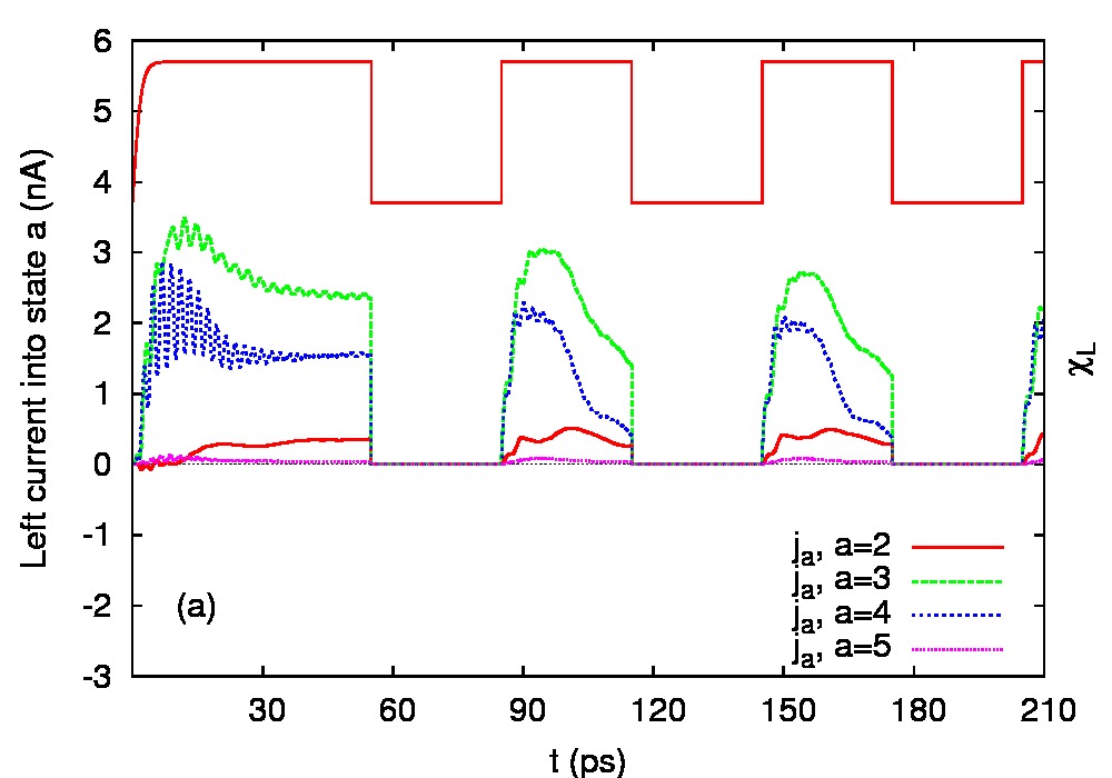
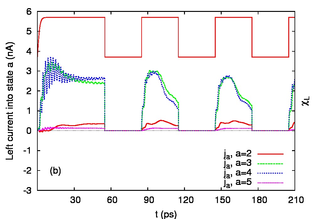
Figure 3: (Color online) The partial current entering the system from the left lead when the bias window contains one respectively two SES. Other parameters: $g_{0}a_{w}^{3/2}=926$ meV, $\delta_{1}a_{w}^{2}=1.0$, $\delta_{2}a_{w}^{2}=2.0$, and $T=60$ ps.

The efficiency of the turnstile operation depends on the pulse length $T$. The previous results are obtained with $T=60$ ps. In those setups the system transfers at least two electrons per cycle. The present GME method is valid in the lowest (quadratic) order of the lead-sample coupling, which means the tunneling of the electrons from the leads to the sample and back is a relatively slow process. Therefore by increasing or decreasing the pulse duration the transferred charge increases or decreases respectively. Denoting by $T_{t}$ the characteristic tunneling time, if $T\leq T_{t}$ the turnstile operation is not expected to work, the allowed time for the charging and discharging of the system being too short. This is the case for $T=10$ ps as shown in Fig. 4, when clearly very little charge can enter and leave the system in a pumping cycle. Actually, the time $T_{t}$ depends on the pairwise coupling (or overlap) of each state of the leads to each state of the sample with energies within the BW. But in order to obtain significant pumping effects, the pulse duration has to include the time of flight (or propagation time) of electrons along the wire. This extra time depends on the energy of the electrons injected from the left lead all the way into the right lead.

Therefore, for a longer pulse, $T=40$ ps, the turnstile pumping process is able to transfer charge through the sample. The occupation number has a triangular shape in time and it becomes periodic after 2-3 cycles. During the initial cycle, which includes the initial charging phase, the system accumulates more than 2 electrons and the steady state is already reached at about 30 ps when the charge in the system is saturated. This is possible because the right contact is still off. The right contact opens for the first time at 45 ps allowing more than 1 electron charge to pass into the right lead. For a longer period, like $T=60$ ps, the occupation number develops toward a saw-tooth profile typical for the charging/relaxation processes. The asymmetry of the charge peaks is determined by the direction of the bias: the electrons leave the sample faster than they entered. The system drives almost two electrons from one lead into the other, which is remarkable given the length of our sample (300 nm).

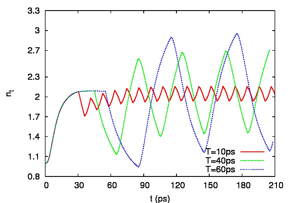
Figure 4: (Color online) The time dependent total occupation of the sample for three pulses at zero magnetic field. The trace for $T=60$ ps is the same as in Fig. 2. Other parameters: $g_{0}a_{w}^{3/2}=926$ meV, $\delta_{1}a_{w}^{2}=1.0$, and $\delta_{2}a_{w}^{2}=2.0$.

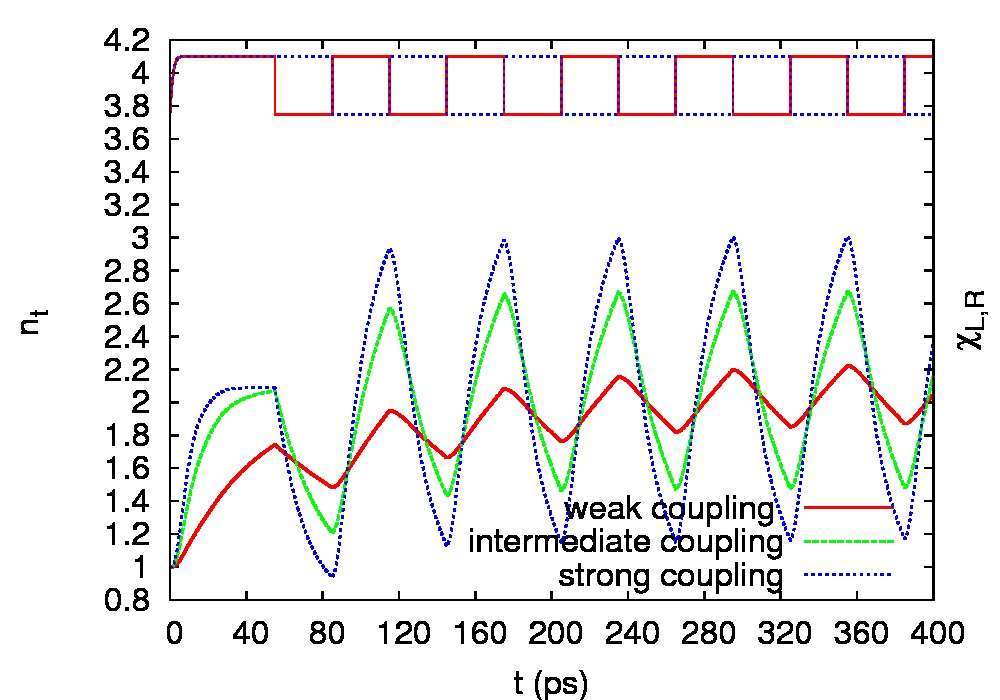
Figure 5: (Color online) The time dependent total occupation for $B=0$ T and two values of the coupling strength. Weak: $g_{0}a_{w}^{3/2}=1408$ meV, $\delta_{1}a_{w}^{2}=1.85$, $\delta_{2}a_{w}^{2}=3.7$. Intermediate: $g_{0}a_{w}^{3/2}=1408$ meV, $\delta_{1}a_{w}^{2}=1.39$, $\delta_{2}a_{w}^{2}=2.77$. Strong: $g_{0}a_{w}^{3/2}=1824$ meV, $\delta_{1}a_{w}^{2}=1.39$, $\delta_{2}a_{w}^{2}=2.77$. The pulse period is $T=60$ ps.

Another important aspect in our model is the strength of the lead-sample coupling, i. e. the parameters $g_{0}$, $\delta_{1}$, and $\delta_{2}$ in Eq. (6). Our GME implementation is restricted to the lowest order in $H_{T}$ (quadratic), supplying the integro-differential equation (5), and thus the parameters have to be appropriately selected. In general it is difficult to evaluate whether the coupling strength is sufficiently low. A necessary (although not sufficient) condition is to obtain positive diagonal elements of the statistical operator, which are the populations of the MES and hence probabilities. Although we always check in our calculations, strictly speaking this condition does not guarantee the validity of the lowest order approximation (quadratic in $H_{T}$). So in practice we cannot avoid choosing our parameters in a semi-empirical manner. To have an idea about the relation between the pumping amplitude and the coupling strength we show in Fig. 5 three calculations done with three strengths of the coupling, which we consider in relative terms weak, intermediate, and strong. In order to compare with the results obtained in the presence of a magnetic field shown in the next examples, the scaled parameters $g_{0}a_{w}^{3/2}$ and $\delta_{1,2}a_{w}^{2}$ are chosen such that the physical values $g_{0}$ and $\delta_{1,2}$ are the same as for $B=0.9$ T. The time dependent occupation of the states in the active window is shown for longer times than in the previous figures to indicate better the final periodic regime. It is not surprising to see that the pumping amplitude increases with the coupling strength, since tunneling of electrons becomes more likely. The same can be said about the current, which is essentially the time derivative of the charge, and it is visible in Fig. 5 that the slope of the charge increases with the coupling strength. The increase of the transient current with the coupling strength has also been shown recently by Sasaoka et al. although in a quantum dot pumping device. Sasaoka

III.2 Magnetic field present

Following our ansatz used to describe the system-leads coupling, Eqs. (3)-(4), we can visualize systems where the physical parameters $g_{0}$, $\delta_{1}$, and $\delta_{2}$ should be assumed constant, and others where the scaled values $g_{0}a_{w}^{3/2}$, $\delta_{1}a_{w}^{2}$, and $\delta_{2}a_{w}^{2}$ should be kept constant with changing values of the magnetic field rather. In the following we explore both possibilities. Our choice of $\Delta_{E}=0.25\hbar\Omega_{w}$ depends also on the value of the magnetic field, but we have checked that variations of this parameter between a scaled version and a fixed physical one will only lead to vanishing quantitative changes in calculations where we consider a range in the $q$ integration of the GME (5) that includes 4 subbands of the leads. This choice of $\Delta_{E}$ guarantees always the same number of subbands in the calculation.

In the presence of a magnetic field, in a first approximation one might expect the amplitude of the charge oscillations to decrease. The reason being that the electronic trajectories bend due to the Lorentz force and the electrons might return to the source lead rather than traveling directly to the drain lead. At the same time we know that a magnetic field generally reduces backscattering. In Fig. 6 where we show the time dependent total charge for different values of the magnetic field we see a reduction of the charge oscillations with increasing magnetic field. For comparison we include the $B=0$ case, also shown in Fig. 2 and Fig. 4. To compare the results with and without magnetic field we initially keep the same coupling parameters as measured with respect to the modified magnetic length, $a_{w}$, i. e. $g_{0}a_{w}^{3/2}=926$, meV $\delta_{1}a_{w}^{2}=1.0$, and $\delta_{2}a_{w}^{2}=2.0$. The modified magnetic length $a_{w}$ decreases with increasing magnetic field, as do the features of the wave functions. We select the bias windows like BW2, with three states included in the window and two marginal states in the extended regions. The energy levels and the wave functions depend on the strength of the magnetic field both in the sample and in the leads. In order to make the comparison shown in Fig. 6 meaningful for each value of the magnetic field we shift the chemical potentials in the leads such that the same energy levels of the quantum wire sample are contained in the bias window with a fixed width.

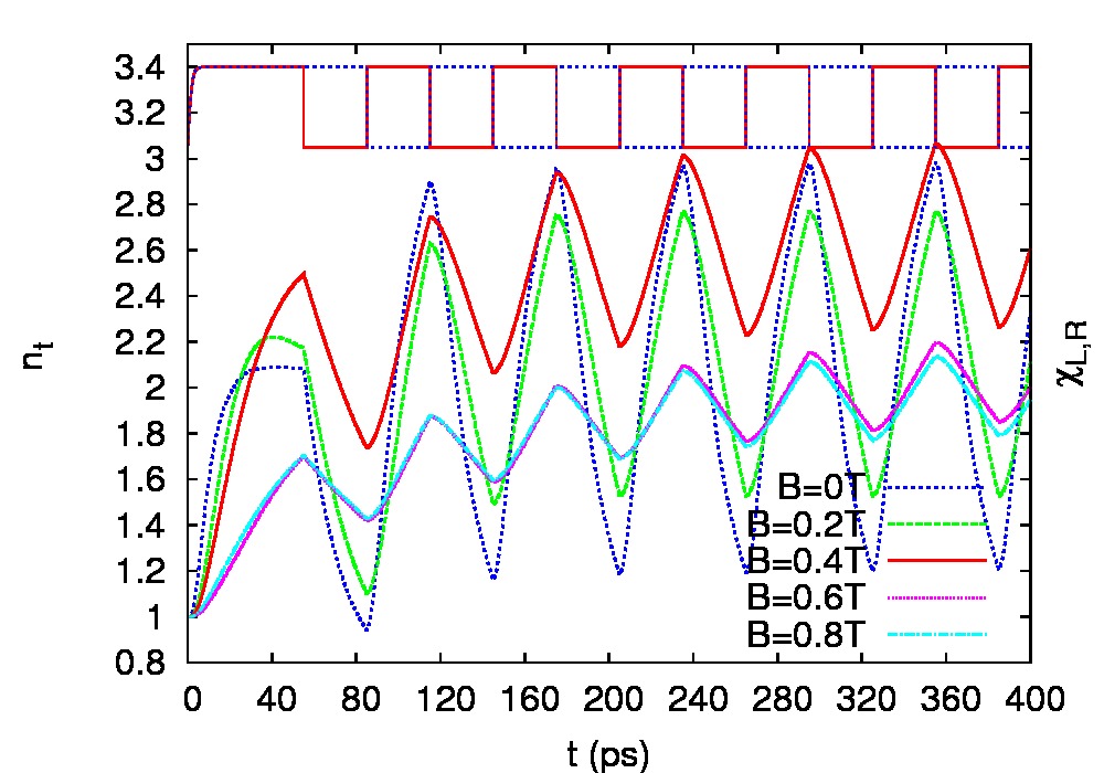
Figure 6: (Color online) The time dependent total occupation of the relevant SESs for different values of the magnetic field. $g_{0}a_{w}^{3/2}=926$ meV, $\delta_{1}a_{w}^{2}=1.0$, $\delta_{2}a_{w}^{2}=2.0$, and $T=60$ ps.

The efficiency of the turnstile pump tends to decrease with increasing the magnetic field. For $B=0$ an amount of charge $Q_{p}\approx 1.8$ electron can be transmitted along the wire sample in one cycle, and for $B=0.2$ T $Q_{p}\approx 1.2$. For stronger magnetic fields $Q_{p}$ drops to 0.8 for $B=0.4$ T, and $Q_{p}<0.5$ at $B>0.6$ T. It is also clear that, at least for the present coupling parameters, the charging time increases in the presence of the magnetic field. During the initial cycle, i. e. for $t<60$ ps, there is less charge accumulated in the system in the normal switching regime than for $B=0$, and also the charging process continues even after the pumping begins. The periodic regime is reached after a number of cycles which increases with $B$.

Although the presence of the magnetic field reduces the electron transfer, the pumped charge still increases with increasing coupling between the leads and the sample. To show that we solve the GME for a fixed magnetic field $B=0.9$ T for three sets of coupling parameters, which we again call (in relative terms) weak, intermediate, and strong coupling, respectively, see Fig. 7. The parameters for the weak coupling are the same as in Fig. 6. For the intermediate coupling we use $g_{0}a_{w}^{3/2}=926$ meV, $\delta_{1}a_{w}^{2}=0.75$, and $\delta_{2}a_{w}^{2}=1.5$. For the strong coupling $g_{0}a_{w}^{3/2}=1200$ meV, $\delta_{1}a_{2}^{2}=0.75$, and $\delta_{2}a_{w}^{2}=1.5$. These parameters correspond to the same physical parameters that were used in Fig. 5. So, if we now compare the results at $B=0.9$ T with the results at $B=0$ we see quite similar charge amplitudes, but somewhat more sensitive to the coupling strength at $B=0.9$ T. For example, at $B=0.9$ T we obtain $Q_{p}\approx 0.4$ electrons at low coupling, $Q_{p}\approx 1.2$ at intermediate coupling, and $Q_{p}\approx 2.4$ at strong coupling. For $B=0$ these numbers are $Q_{p}\approx 0.3,1.2$, and $1.8$, as can be read from Fig. 5.

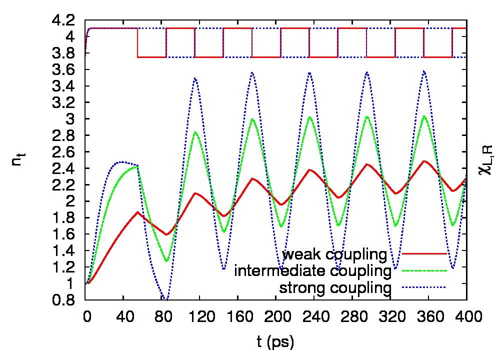
Figure 7: (Color online) The time dependent total occupation for $B=0.9T$ and three coupling strength: weak ($g_{0}a_{w}^{3/2}=926$ meV, $\delta_{1}a_{w}^{2}=1.0$, and $\delta_{2}a_{w}^{2}=2.0$, intermediate ($g_{0}a_{w}^{3/2}=926$ meV, $\delta_{1}a_{w}^{2}=0.75$, and $\delta_{2}a_{w}^{2}=1.5$), and strong ($g_{0}a_{w}^{3/2}=1200$, $\delta_{1}a_{w}^{2}=0.75$, and $\delta_{2}a_{w}^{2}=1.5$). The pulse period is $T=60$ ps.

We believe the increased sensitivity of the pumping to the contact strength in the presence of the magnetic field is a result of the edge states created in the sample. The edge states are indeed more and more pronounced with increasing magnetic field, and so is the pumped charge if the edge states are in good overlap with the coupling region. Therefore with magnetic fields of about 1 T and strong coupling we can obtain $Q_{p}$ of about 2 electrons, Fig. 8, which is slightly more than at zero magnetic field but with weak coupling $Q_{p}\approx 1.75$, visible in Fig. 7.

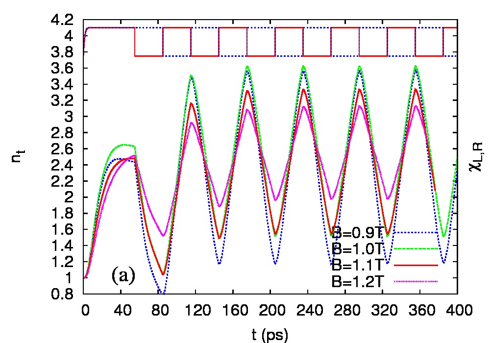
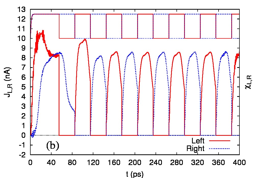
Figure 8: (Color online) (a) The time dependent total occupation of the relevant SESs for $B=0.9-1.2$ T. (b) The total current entering the system from the left lead and the total current exiting the system into the right lead for $B=1.0$ T. Parameters: $g_{0}a_{w}^{3/2}=1200$ meV, $\delta_{1}a_{w}^{2}=0.75$, and $\delta_{2}a_{w}^{2}=1.5$. The pulse period $T=60$ ps.

The time dependent total currents in the left and right leads are shown in the lower panel of Fig. 8 for $B=1$ T. The currents suddenly vanish at each contact when the contact is closed. The currents have a trapezoidal shape for the pulse duration $t=60$ ps, but they become triangular for shorter pulses like $T=10$ ps (not shown).

III.3 Analysis of edge states

Clearly, states in the sample with higher probability at the contact edges contribute more to the pumping. In Fig. 9 we show the coupling strength of each of the five states of the finite wire involved in the transport for each magnetic field of Fig. 8, only for the lowest subband of the leads. The general trend of the coupling coefficients is to decrease with increasing magnetic field. So the decrease of the pumping when the magnetic field increases can be explained by the decrease of the coupling strength. The contribution of each state to the transport is given by an integration over all the lead states $q$ in the GME.

To see the contribution of each state to the transport we show in Fig. 10 the time dependent occupation of all 5 states included in the calculation for $B=1.2$ T, which are the states number 6-10 in the single-electron energy spectrum of the finite wire. It is clear that the three middle states $a=7,8,9$ contribute unequally to the pumping. These states are well inside the BW, but the coupling energies are slightly different as seen in Fig. 9 for $B=1.2$ T. For the other values of the magnetic field shown in Fig. 9 the states within the BW have nearly equal coupling to the leads and consequently nearly equal contributions to transport. So in general the coupling strength may depend on the state and so does the corresponding partial current. The states 6 and 10 included in Fig. 10 are slightly outside the BW and obviously their contribution to transport is smaller.

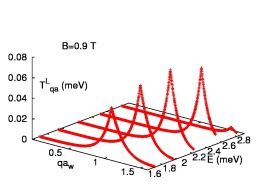
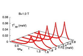
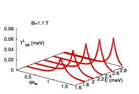
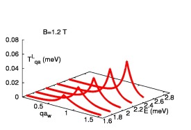
Figure 9: (Color online) The coupling energies between the states $a=6-10$ and states of the lowest subband in the left (or the right) lead for $B=0.9-1.2$ T. $g_{0}a_{w}^{3/2}=1200$ meV, $\delta_{1}a_{w}^{2}=0.75$, and $\delta_{2}a_{w}^{2}=1.5$.

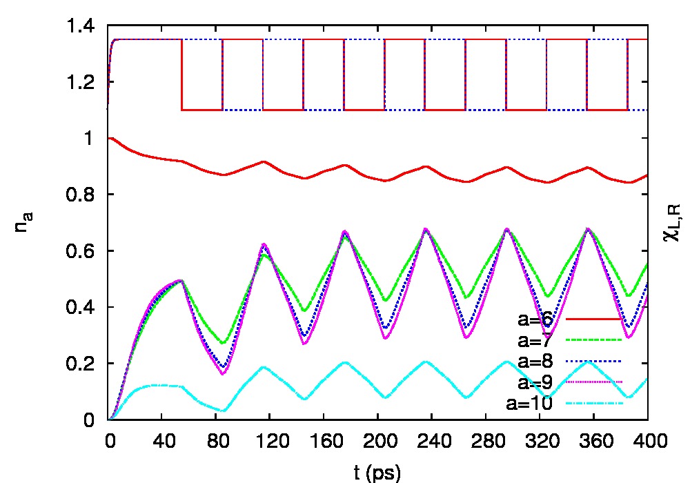
Figure 10: (Color online) The time dependent total occupation of the relevant SESs for $B=1.2$ T. $g_{0}a_{w}^{3/2}=1200$ meV, $\delta_{1}a_{w}^{2}=0.75$, and $\delta_{2}a_{w}^{2}=1.5$. $T=60$ ps.

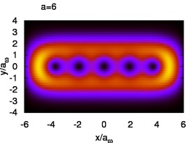
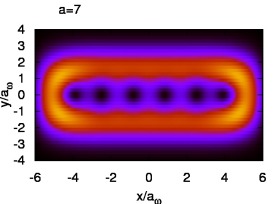
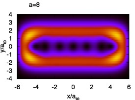
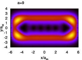
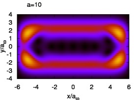
Figure 11: (Color online) The probability density of the single-electron eigenstates of the sample number 6-10 (top left - right - down), for $B=1$ T.

In Fig. 11 we show the probability density associated to the five active single-electron states (number 6-10) of the finite quantum wire. The figures indicates that all the five states have the characteristics of an edge state. In vanishing magnetic field the probability density of the active states is on the average smeared over the finite wire. As the magnetic field increases the Lorentz force squeezes the probability of some states close to the edge of the finite wire. This also happens at the hard-wall ends of the wire, the contact area. This fact explains why the increasing of the coupling through increasing $g_{0}$ should be more effective at high magnetic field. From Fig. 11 it is evident that the edge states will have different coupling strengths to the leads due to the difference in their finer structure in the contact area. This finer structure in the contact area of the wire induces differential coupling to the states in the different subbands of the leads.

The time-dependent charge in the quantum wire is shown in Fig. 12 for the parameters used in Fig. 8b. The charge distribution reflects the geometry of the quantum wire and of the five SESs involved, and indicates the propagation of the electrons in the system. The selected time moments cover the initial charging cycle plus a part of the next cycle. It is interesting to observe how the electrons are injected at the left contact into the sample traveling along the quantum wire on the upper edge channel, and how they are reflected back at the right contact traveling along the lower channel.

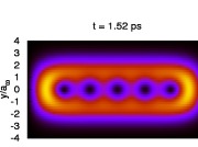
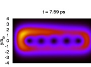
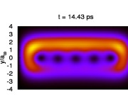
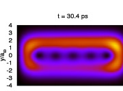
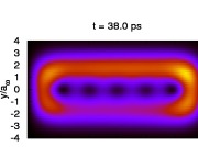
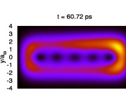
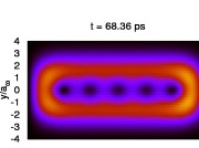
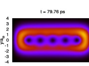
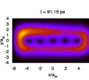
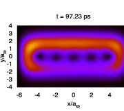
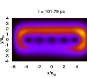
Figure 12: (Color online) The average spatial charge distribution in the quantum wire for $B=1$ T with strong coupling, at different moments of time.

IV Conclusions

The turnstile conduction of a two-dimensional parabolic wire, seen as “the sample”, attached to semi-infinite leads of a similar parabolic shape has been studied using a non-Markovian generalized master equation method. This system is far more complex than the simple two- or three-level system with one-dimensional leads considered in an earlier publication based on the Keldysh-Green functions approach.TSPPRB The eigenstates of the leads and of the finite wire have been calculated in an external perpendicular magnetic field using a combination of analytical and numerical methods for large functional basis sets. We have taken into account the subband structure of the leads to which it is attached. We have also described phenomenologically the coupling coupling between the states in the leads and the states in the finite wire as a nonlocal overlap of the wave functions from both sides of the contact.

We have analyzed the effects of the bias window, pulse length, and magnetic field on the evolution in time of the number of electrons in the sample. We have found that longer pulses are more favorable for the turnstile pumping as the electrons need time to propagate along the sample wire. One or two electrons could be transferred through the 300 nm wire using pulses of 40 or 60 ps.

The comparison of the results obtained with and without a magnetic field is a difficult issue. If a magnetic field is present all energies shift, all wave functions change (both in the sample and in the leads), and also all elements of the coupling tensor $T_{qa}^{l}$ between lead and sample states change. Of course these changes depend on the strength of the field. Therefore it is difficult to create similar conditions for two different field values, i. e. the same number of states in the bias window and the same coupling energies, in order to compare only the amplitude of the pumped charge. To do that we have selected the parameters describing the phenomenological coupling of the leads to the finite wire in two different ways, both scaled and not scaled with the effective width of the sample, which implicitly depends on the magnetic field. This is an issue that can only be better resolved with a more involved microscopic model of the coupling and comparison to experiments where the coupling strength could be varied, for example by using finger-strip gates.

The charge distribution inside the system, Fig. 12, emphasizes the dynamics induced by the charging/discharging sequences. The charge propagation along edge-states in a strong magnetic field indicates that the optimal turnstile period depends on the external magnetic field. Experimental studies of turnstile pumping in quantum wires have to clarify the relationship between the magnetic field, pumping amplitude, and contact strength.

- (1) T. Fujisawa, D. G. Austing, Y. Tokura, Y. Hirayama, S. Tarucha, J. Phys. Cond. Mat. 15, R1395 (2003).
- (2) W.-T. Lai, D. M. T. Kuo, and P.-W. Li, Physica E 41, 886 (2009).
- (3) B. Naser, D. K. Ferry, J. Heeren, J. L. Reno, and J. P. Bird, Appl. Phys. Lett. 89, 083103 (2006); 90, 043103 (2007).
- (4) G. Stefanucci, S. Kurth, A. Rubio and E. K. U. Gross, Phys. Rev. B 77, 075339 (2008).
- (5) V. Moldoveanu, A. Manolescu and V. Gudmundsson, Phys. Rev. B 76, 085330 (2007)
- (6) V. Gudmundsson, G. Thorgilsson, C-S Tang, and V. Moldoveanu, Phys. Rev. B 77, 035329 (2008).
- (7) U. Harbola, M. Esposito, and S. Mukamel, Phys. Rev. B 74, 235309 (2006).
- (8) V. Moldoveanu, V. Gudmundsson, and A. Manolescu, N. J. Phys. 11, 073019 (2009).
- (9) S. Welack, M. Schreiber, and U. Kleinekathöfer, J. Chem. Phys. 124, 044712 (2006)
- (10) V. Gudmundsson, C. Gainar, C.-S. Tang, V. Moldoveanu, and A. Manolescu, New J. Phys. 11, 11300 7 (2009).
- (11) V. Moldoveanu, A. Manolescu, V. Gudmundsson, Phys. Rev. B 80, 205325 (2009).
- (12) L. P. Kouwenhoven, A. T. Johnson, N. C. van der Vaart, C. J. P. M. Harmans, and C. T. Foxon, Phys. Rev. Lett. 67, 1626 (1991).
- (13) Y. Mizugaki, J. Appl. Phys. 94, 4480 (2003).
- (14) H. Ikeda and M. Tabe, J. Appl. Phys. 99, 073705 (2006).
- (15) V. Moldoveanu, V. Gudmundsson, and A. Manolescu,Phys. Rev. B 76, 165308 (2007).
- (16) K. Sasaoka, T. Yamamoto, and S. Watanabe, Appl. Phys. Lett. 96, 102105 (2010).