Controllability on relaxation-free subspaces: On the relationship between adiabatic population transfer and optimal control

Abstract

We consider the optimal control problem of transferring population between states of a quantum system where the coupling proceeds only via intermediate states that are subject to decay. We pose the question whether it is generally possible to carry out this transfer. For a single intermediate decaying state, we recover the Stimulated Raman Adiabatic Passage (STIRAP) process which we identify as the global optimum in the limit of infinite control time. We also present analytical solutions for the case of transfer that has to proceed via two consecutive intermediate decaying states. We show that in this case, for finite power the optimal control does not approach perfect state transfer even in the infinite time limit. We generalize our findings to characterize the topologies of paths that can be achieved by coherent control under the assumption of finite power. If two or more consecutive states in an $N$-level chain are subject to decay, complete population transfer with finite-power controls is not possible.

I Introduction

Stimulated Raman adiabatic passage (STIRAP) achieves coherent population transfer in three-level atoms or molecules despite the short lifetime of the intermediate level Bergmann et al. (1998). The key is the creation of a dark state produced by overlapping pump and Stokes pulses in a counter-intuitive sequence. In the adiabatic limit, the intermediate state then never gets populated. STIRAP was first demonstrated two decades ago Gaubatz et al. (1990) but it continues to enjoy great popularity due to its simple, yet robust character Lang et al. (2008); Ni et al. (2008).

Inspired by this, we consider the general $N$-level system with a subspace that is free of relaxation, as shown in Fig. 1.

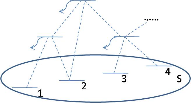
Figure 1: (Color online) A general $N$-level system where the states in the subspace $S$ are connected through intermediate states outside of $S$.

We consider the case that there is no direct coupling between states in the relaxation-free subspace, but the states are coupled by intermediate states that undergo relaxation. The question we ask here is what kind of coupling topology can ensure state-to-state controllability on the relaxation-free subspace? We show that this question can be reduced to asking what kind of coupling topology can ensure unit efficiency of population transfer for any two eigenstates in the relaxation-free subspace.

Our work is closely related to previous studies of STIRAP in multi-level chains Shore et al. (1991); Malinovsky and Tannor (1997); Vitanov et al. (1998); Nakajima (1999) which showed that under certain assumptions the dark state condition can be generalized from the three-level to the $N$-level case. In these studies, the decay from intermediate levels was not explicitly taken into account. Here, we include the dissipation. Moreover, we use an analytical formulation of optimal control theory which allows us to draw striking general conclusions about $N$-level systems. In particular, we are able to show a relationship between controllability and connectivity of decaying states in the chain: A relaxation-free subspace is controllable on the pure state space if and only if any two eigenstates in the subspace can be connected by a path that never visits two consecutive states that both suffer relaxation. This coupling topology includes degenerate levels provided that a generalized Morris-Shore transformation exists to replace the coupled multi-level system by a set of two- and three-level systems and single dark states Rangelov et al. (2006).

The problem of controllability in a relaxation-free subspace is closely related to fault tolerant quantum computing and decoherence-free subspaces in quantum information science. Given that the Hamiltonian obeys a certain symmetry, two or more physical qubits can be employed to encode one logical qubit that is free of decoherence Lidar and Whaley (2003). The condition for a dark state ensuring STIRAP turns out to be equivalent to the condition for a decoherence-free subspace to exist Lidar and Whaley (2003). While in principle it is possible to construct quantum gates that preserve the structure of the decoherence free subspace Monz et al. (2009), these gates are generally difficult to implement in practice for the following reason: the gate operations need to be carried out with controls that act on the physical qubits and this introduces couplings to the decohering subspaces Fortunato et al. (2002). This raises the question of whether losses can still be avoided if the controls are chosen in an optimal way. Previous work has discussed whether optimal control can find STIRAP-like solutions in $N$-level chains Band and Magnes (1994); Wang and Rabitz (1996); Malinovsky and Tannor (1997); Solá et al. (1999); Kis and Stenholm (2002); Boscain et al. (2002). However, none of these studies took the dissipation explicitly into account.

Our paper is organized as follows. In section II, we study the three-level system. Using optimal control theory we show that a STIRAP-like process represents the globally optimal process for the population transfer in the relaxation-free subspace. This STIRAP-like process is the infinite time limit of analytic solutions we find for the problem with finite time. In section III, we study a four-level chain system where the two intermediate states are subject to decay. We show that with limited pulse power, it is not possible to achieve complete population transfer. Section IV generalizes these results to $N$-level chains. This generalization is used in section V to state the conditions on state-to-state controllability on the relaxation-free subspace. Section VI concludes.

II Three-level system

We consider a three-level $\Lambda$-system with states $|1\rangle$, $|2\rangle$, $|3\rangle$ where $|2\rangle$ suffers relaxation loss with rate $k$. It is well known that population transfer from $|1\rangle$ to $|3\rangle$ is possible by STIRAP without populating state $|2\rangle$, i.e., complete transfer is achieved in the adiabatic limit Bergmann et al. (1998). In this section, we formulate the population transfer as an optimal control problem, taking the dissipation explicitly into account. Previous work has addressed this problem using a numerical density matrix optimization Hornung et al. (2002). Here, we formulate the problem analytically using the Hamilton-Jacobi-Bellman method which has the additional advantage of allowing us to determine the global optimum. We will show that STIRAP arises naturally as the solution to the optimal control problem in the adiabatic limit. By yielding an upper bound for the transfer efficiency in finite time, this formulation also gives some insight into the three-level system in the non-adiabatic regime.

The dynamics of the three-level system are described by the following effective Schrödinger equation,

$$\frac{d}{dt}\left(\begin{array}[]{c}x^{\prime}_{1}\\ x^{\prime}_{2}\\ x^{\prime}_{3}\end{array}\right)=-i\left(\begin{array}[]{ccc}0&\Omega_{p}&0\\ \Omega_{p}&-ik&\Omega_{s}\\ 0&\Omega_{s}&0\end{array}\right)\left(\begin{array}[]{c}x^{\prime}_{1}\\ x^{\prime}_{2}\\ x^{\prime}_{3}\end{array}\right)$$ (1)

where we assume that the detuning is zero. $\Omega_{p}$ and $\Omega_{s}$ are half the Rabi frequencies of the pump and Stokes pulses , and $k$ is the decay rate of state $|2\rangle$. We want to optimize the transfer of population from $|1\rangle$ to $|3\rangle$ within a given time $T$, i.e., to steer the system from the initial state $|\phi(0)\rangle=(1,0,0)$ to the final state $|\phi(T)\rangle$ such that $|x^{\prime}_{3}(T)|$ is maximized.

We first make a change of variables, setting $x_{1}=x_{1}^{\prime}$, $x_{2}=ix^{\prime}_{2}$, $x_{3}=-x_{3}^{\prime}$. The dynamics becomes

$$\frac{d}{dt}\left(\begin{array}[]{c}x_{1}\\ x_{2}\\ x_{3}\end{array}\right)=\left(\begin{array}[]{ccc}0&-\Omega_{p}&0\\ \Omega_{p}&-k&-\Omega_{s}\\ 0&\Omega_{s}&0\end{array}\right)\left(\begin{array}[]{c}x_{1}\\ x_{2}\\ x_{3}\end{array}\right)\,.$$ (2)

Under these dynamics, if we start from the initial state $(1,0,0)$, all the state variables will remain real, i.e., this change of variables is motivated by the structure of the Schrödinger equation and the fact that we are looking for state-to-state control. Initial states such as $(e^{i\varphi},0,0)$ can be written as $e^{i\varphi}(1,0,0)$, and since quantum operations act linearly on the states, these cases can be reduced to the $(1,0,0)$ case. The goal is to transfer population from $(1,0,0)$ to the final state such that $x_{3}(T)$ is maximized under the controls $\Omega_{p}$ and $\Omega_{s}$.

In a realistic setup, both pump and Stokes pulses are limited in amplitude, but we will relax this condition: we assume that $\Omega_{s}$ is bounded in amplitude by $A$ while $\Omega_{p}$ is unbounded. This assumption enables us to solve the problem analytically and yields an upper bound on the transfer efficiency. Since the amplitude of the pulses is usually quite large compared to the relaxation rate, these upper bounds are quite tight. We will also show that in the adiabatic limit, the condition of unbounded $\Omega_{p}$ can be relaxed and STIRAP-like pulses arise naturally from the solution of the optimal control problem.

II.1 Optimal solution

To find the optimal pulses, we make another change of variables, setting $r_{1}=\sqrt{x^{2}_{1}+x^{2}_{2}}$, $r_{2}=x_{3}$, and $\tan\theta=\frac{x_{1}}{x_{2}}$, where $\theta\in[0,\frac{\pi}{2}]$. The dynamics for $(r_{1},r_{2})$ are derived from Eq.(2),

$$\frac{d}{dt}\left(\begin{array}[]{c}r_{1}\\ r_{2}\\ \end{array}\right)=\left(\begin{array}[]{cc}-k\cos^{2}\theta&-\Omega_{s}\cos\theta\\ \Omega_{s}\cos\theta&0\\ \end{array}\right)\left(\begin{array}[]{c}r_{1}\\ r_{2}\\ \end{array}\right)\,.$$ (3)

Note that $\Omega_{p}$ is now contained in $\theta$ and $r_{1}$ is related to the bright-state amplitude in STIRAP. This change of variables is not intuitive but crucial for obtaining an analytical solution. For equations of motion linear in the control, the optimal control problem typically becomes singular and no conditions to determine an analytical solution are obtained. After this change of variables, the equations of motion are non-linear in one of the controls, $\cos\theta$. This will allow us to obtain a non-vanishing condition determining the optimal solution when applying Pontryagin’s maximum principle.

Considering the physics of the problem we find that $\Omega_{s}$ should take on the maximal amplitude $A$ throughout the process: We start from the initial state $(r_{1},r_{2})=(1,0)$ and want to maximize $r_{2}(T)$. The population transfer between $r_{1}$ and $r_{2}$ depends on the rotation speed which is determined by $\Omega_{s}\cos\theta$. At the same time, the population transfer is compromised by $r_{1}$ undergoing decay. The effect of decay on $r_{1}$ can be decreased by lowering the value of $\cos\theta$. In order to keep the rotation speed between $r_{1}$ and $r_{2}$ constant, $\Omega_{s}$ needs to be increased. For a given rotation speed, the minimum value of $\cos\theta$ and thus the minimum effect of the decay is obtained for $\Omega_{s}$ taking its maximum value, $\Omega_{s}=A$.

We are now left with determining $\Omega_{p}$, or, equivalently, the angle $\theta$. Defining $u=\cos\theta$, we rewrite the dynamics

$$\frac{d}{dt}\left(\begin{array}[]{c}r_{1}\\ r_{2}\\ \end{array}\right)=\left(\begin{array}[]{cc}-ku^{2}&-Au\\ Au&0\\ \end{array}\right)\left(\begin{array}[]{c}r_{1}\\ r_{2}\\ \end{array}\right).$$ (4)

To determine the optimal control $u^{*}(t)$, we use the principle of dynamic programming Bertsekas (2005) and solve for the maximum achievable value of $r_{2}(T)$ for all initial points $(r_{1},r_{2})$. Starting from $(r_{1},r_{2})$, we denote the maximum achievable value of $r_{2}$ by $V(r_{1},r_{2},t)$, also called the optimal return function for the point $(r_{1},r_{2})$ at time t. Note that for finite time problems, $T<\infty$, the optimal return function has an explicit dependence on time, which has to satisfy the well known Hamilton-Jacobi-Bellman equation,

$$\frac{\partial V}{\partial t}+\max_{u}H(u)=0\,,$$ (5)

where

$$H(u)=\left(\begin{array}[]{cc}\frac{\partial V}{\partial r_{1}}&\frac{\partial V}{\partial r_{2}}\\ \end{array}\right)\left(\begin{array}[]{cc}-ku^{2}&-Au\\ Au&0\\ \end{array}\right)\left(\begin{array}[]{c}r_{1}\\ r_{2}\\ \end{array}\right)$$ (6)

is the Hamiltonian of the optimal control problem.

By solving the Hamilton-Jacobi-Bellman equation, we obtain the optimal solution to the control problem. The detailed derivation is presented in Appendix A. Here we just state the results we need for the subsequent analysis. For control time $T$ longer than a critical time $T_{M}$ the optimal control has two distinct phases:

$$u^{*}(t)=\left\{\begin{array}[]{lc}\frac{1}{\sqrt{A^{2}(\tau^{2}-t^{2})+2k(\tau-t)+1}}&\textrm{for $t\in[0,\tau]$}\\ 1&\textrm{for $t\in[\tau,T]$}\\ \end{array}\,,\right.$$ (7)

Expressions for $T_{M}$ and $\tau$ are given in Appendix A. The second stage of this solution, $u^{*}(t)=1$, is a result of the artificial choice of constraints in our formulation (bounded $\Omega_{S}$ and unbounded $\Omega_{P}$). But this need not concern us: as we show in Section II.2 the second phase of the solution vanishes in the limit $T\to\infty$ (adiabatic limit), in which case we recover the STIRAP solution.

II.2 Recovery of STIRAP

We now show that in the limit $T\to\infty$, our optimal pulse corresponds to STIRAP. The optimal Rabi frequencies are derived from $r_{1}$, $r_{2}$ and $u^{*}$. From Eq.(2), it follows that

$$\frac{d}{dt}x_{2}=\Omega_{p}x_{1}-kx_{2}-\Omega_{s}x_{3}\,.$$ (8)

Substituting $x_{2}=r_{1}u$, $x_{1}=r_{1}\sqrt{1-u^{2}}$, and $x_{3}=r_{2}$, we obtain

$$\Omega_{p}=\frac{-ku^{2}r_{1}-\Omega_{s}ur_{2}+r_{1}\dot{u}+kr_{1}u+\Omega_{s}r_{2}}{r_{1}\sqrt{1-u^{2}}}\,.$$ (9)

When the control time goes to infinity, $T\rightarrow\infty$, the switching time, $\tau$, also approaches $\infty$. This follows from $T-\tau$ being smaller than the critical time $T_{M}$ as explained in Appendix A. If $\tau$ becomes very large, then according to Eq. (7), $u^{*}(t)$ is very small. Therefore $x_{2}=r_{1}u^{*}\sim 0$, i.e., the level $|2\rangle$ is not populated. Substituting $u\sim 0$ and $\dot{u}\sim 0$ into Eq. (9), we see that

$$\Omega_{p}=\frac{r_{2}}{r_{1}}\Omega_{s}=\frac{x_{3}}{\sqrt{x_{1}^{2}+x_{2}^{2}}}\Omega_{s}=\frac{x_{3}}{x_{1}}\Omega_{s}\,.$$ (10)

So at each time point, $x_{2}=0$, $\frac{x_{3}}{x_{1}}=\frac{\Omega_{p}}{\Omega_{s}}$, i.e., the system is in the state $x_{1}|1\rangle+x_{3}|3\rangle$, where $\frac{x_{3}}{x_{1}}=\frac{\Omega_{p}}{\Omega_{s}}$, which corresponds to the dark state in STIRAP.

Note that in this limit, an upper bound can also be assumed for $\Omega_{p}$ in addition to the one for $\Omega_{s}$. Since it is the ratio $\Omega_{p}/\Omega_{s}$ that matters, one can simply lower $\Omega_{s}$ if $\Omega_{p}$ exceeds its upper bound to maintain the ratio $\Omega_{p}/\Omega_{s}$. For example, one could assume the same bound $A$ on $\Omega_{p}$. In the optimal solution shown in Fig. 2, one would then rescale time whenever $\Omega_{p}$ hits $A$. This obviously avoids the shoot-off of $\Omega_{p}$ to infinity visible in Fig. 2

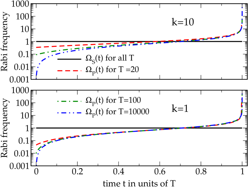
Figure 2: (Color online) Optimal half Rabi frequencies $\Omega_{S}(t)$ and $\Omega_{P}(t)$ for finite control times $T$ and relaxation rates $k$ (with the amplitude bound on $\Omega_{S}$ set to one, $A=1$).

at late times. Such a rescaling of amplitude corresponds to changing the unit of time: When $\Omega_{p}\geq A$, a new time variable $d\tau=\frac{\Omega_{p}}{A}dt$ is defined. In this new unit of time, the dynamics become

$$\frac{d}{d\tau}\left(\begin{array}[]{c}x_{1}\\ x_{2}\\ x_{3}\end{array}\right)= \frac{d}{dt}\left(\begin{array}[]{c}x_{1}\\ x_{2}\\ x_{3}\end{array}\right)\frac{dt}{d\tau}$$ (11)

$$= \left(\begin{array}[]{ccc}0&-A&0\\ A&-\frac{A}{\Omega_{p}}k&-\frac{A}{\Omega_{p}}\Omega_{s}\\ 0&\frac{A}{\Omega_{p}}\Omega_{s}&0\end{array}\right)\left(\begin{array}[]{c}x_{1}\\ x_{2}\\ x_{3}\end{array}\right).$$

The relaxation rate $k$ does not affect the dynamics in the infinite time limit, so $k$ and $\frac{A}{\Omega_{p}}k$ are effectively the same, and the ratio of the Rabi frequencies still satisfies the optimal condition in Eq. (10). Since the reparametrized time remains infinite in the limit $T\rightarrow\infty$, optimality of our solution is not affected by changing the unit of time.

One might wonder in this case where the characteristic time delay between $\Omega_{s}$ and $\Omega_{p}$ is hidden in our solution. The point is that STIRAP is determined by the overlap of the pulses. The rising part of the Stokes pulse when the pump is zero and the falling part of the pump pulse when the Stokes is zero do not affect the system dynamics. Our solution only contains the crucial overlapping part, similar to the ”shark-fin” pulses discussed in Ref. Yatsenko et al. (1998). The Stokes pulse starts out fairly flat at the upper bound and falls down as the pump pulse is rising up to the bound. So the delay between the pulses in standard STIRAP corresponds to the time the pump pulse takes to rise to the upper bound. In our solution, a rising edge of the Stokes pulse and a falling edge of the pump pulse could be added if one wishes to obtain a more realistic pulse shape.

To summarize the similarities and differences with the conventional STIRAP solution, we drop the constraint on the bound of the pulse amplitude $\Omega_{p}$ and obtain an analytical solution for the optimal control (cf. Eqs. (7),(9)) in finite time. While in general the optimal pulse shape can be found only numerically, for infinite time we obtain a completely analytical solution (cf. Eq. (10)). By solving the Hamilton-Jacobi-Bellman equation, we have proven that this solution is the global optimum. The rise of the Stokes pulse and the fall of the pump pulse are missing. These portions of the pulses are irrelevant in the infinite time limit. Thus, our analytical solution confirms that the essential feature of STIRAP is the time-ordering of the pump and Stokes pulse where they overlap.

III Four-level system

In this section, we extend our method to a four-level chain system as shown in Fig. 3. Again we explicitly include the decay from the intermediate levels. We can thus demonstrate that the four-level chain differs fundamentally from the three-level system where STIRAP-like processes can transfer the population fully in the adiabatic limit. It turns out that in four-level systems with two decaying intermediate states it is not possible to achieve complete transfer with limited power even if we wait infinite time.

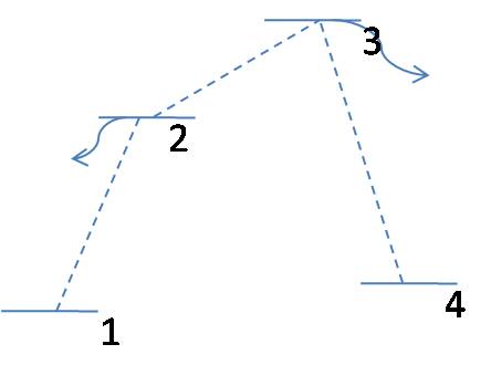
Figure 3: (Color online) A four-level system: Population shall be transferred from $|1\rangle$ to $|4\rangle$ via the intermediate states $|2\rangle$ and $|3\rangle$ which suffer relaxation.

The dynamics of this system are described by the following effective Schrödinger equation,

$$\frac{d}{dt}\left(\begin{array}[]{c}x^{\prime}_{1}\\ x^{\prime}_{2}\\ x^{\prime}_{3}\\ x^{\prime}_{4}\end{array}\right)=-i\left(\begin{array}[]{cccc}0&\Omega_{p}&0&0\\ \Omega_{p}&-ik&\Omega_{I}&0\\ 0&\Omega_{I}&-ik&\Omega_{s}\\ 0&0&\Omega_{s}&0\end{array}\right)\left(\begin{array}[]{c}x^{\prime}_{1}\\ x^{\prime}_{2}\\ x^{\prime}_{3}\\ x^{\prime}_{4}\end{array}\right)\,,$$ (12)

where $\Omega_{p}$ and $\Omega_{s}$ are the Rabi frequencies of pump and Stokes pulses, $\Omega_{I}$ is the Rabi frequency of a pulse coupling $|2\rangle$ and $|3\rangle$, and $k$ denotes the decay rate. As in the previous section, we assume zero detunings. Since we are only interested to find out whether there are schemes which avoid populating the intermediate states, the exact value of the relaxation rate is not important here. For simplicity, we assume that the intermediate states suffer the same amount of relaxation. It is straightforward to generalize to the cases with different decay rates.

We want to find the optimal way to transfer population from $|1\rangle$ to $|4\rangle$ within a given time $T$, i.e., the optimal way of steering the system from the initial state $|\phi(0)\rangle=(1,0,0,0)$ to the final state $|\phi(T)\rangle$ such that $|x^{\prime}_{4}(T)|$ is maximized.

Analogously to Section II, we make a first change of variables, letting $x_{1}=x_{1}^{\prime}$, $x_{2}=ix^{\prime}_{2}$, $x_{3}=-x_{3}^{\prime}$, $x_{4}=-ix_{4}^{\prime}$. The dynamics become

$$\frac{d}{dt}\left(\begin{array}[]{c}x_{1}\\ x_{2}\\ x_{3}\\ x_{4}\end{array}\right)=\left(\begin{array}[]{cccc}0&-\Omega_{p}&0&0\\ \Omega_{p}&-k&-\Omega_{I}&0\\ 0&\Omega_{I}&-k&-\Omega_{s}\\ 0&0&\Omega_{s}&0\end{array}\right)\left(\begin{array}[]{c}x_{1}\\ x_{2}\\ x_{3}\\ x_{4}\end{array}\right)\,.$$ (13)

The state variables are now all real numbers if we start from the initial state $(1,0,0,0)$. We want to transfer from $(1,0,0,0)$ to the final state such that $x_{4}(T)$ is maximized under the controls $\Omega_{p}$, $\Omega_{I}$ and $\Omega_{s}$ at given time $T$. We again relax the control constraint, assuming that $\Omega_{I}$ is bounded in amplitude by $A$, but $\Omega_{p}$ and $\Omega_{s}$ are not bounded. We show that even with these relaxed control constraints, it is not possible to achieve unit transfer efficiency.

To solve the problem, we make a second change of variables, letting $r_{1}=\sqrt{x_{1}^{2}+x_{2}^{2}}$, $r_{2}=\sqrt{x_{3}^{2}+x_{4}^{2}}$, $\tan\theta_{1}=\frac{x_{1}}{x_{2}}$, $\tan\theta_{2}=\frac{x_{4}}{x_{3}}$. The dynamics of $(r_{1},r_{2})$ become

$$\frac{d}{dt}\left(\begin{array}[]{c}r_{1}\\ r_{2}\\ \end{array}\right)=\left(\begin{array}[]{cc}-k\cos^{2}\theta_{1}&-\Omega_{I}\cos\theta_{1}\cos\theta_{2}\\ \Omega_{I}\cos\theta_{1}\cos\theta_{2}&-k\cos^{2}\theta_{2}\\ \end{array}\right)\left(\begin{array}[]{c}r_{1}\\ r_{2}\\ \end{array}\right)\,.$$ (14)

This looks familiar since we have almost the same equation as for three-level system, cf. Eq.(3). We first observe that $\Omega_{I}$ should always take on the maximal amplitude $A$: if $\Omega_{I}<A$, we can always increase it to $A$ while lowering $\cos\theta_{1}$ and $\cos\theta_{2}$ such that the rotation speed $\Omega_{I}\cos\theta_{1}\cos\theta_{2}$ remains the same, but the effect of decay on $r_{1}$, $r_{2}$ is decreased. The problem therefore reduces to

$$\frac{d}{dt}\left(\begin{array}[]{c}r_{1}\\ r_{2}\\ \end{array}\right)=\left(\begin{array}[]{cc}-ku_{1}^{2}&-Au_{1}u_{2}\\ Au_{1}u_{2}&-ku_{2}^{2}\\ \end{array}\right)\left(\begin{array}[]{c}r_{1}\\ r_{2}\\ \end{array}\right)\,,$$ (15)

where $u_{1}=\cos\theta_{1}$ and $u_{2}=\cos\theta_{2}$. The same dynamics arise in Nuclear Magnetic Resonance and analytical solutions to this control problem were obtained using the optimal control technique in Ref. Khaneja et al. (2003). We describe the characteristics of the optimal pulse sequences and refer to Ref. Khaneja et al. (2003) for more details.

Case I: If $T\leq{{\cot^{-1}(2\xi)}\over{A}}$, where $\xi=\frac{k}{A}$, then $u_{1}^{*}(t)=u_{2}^{*}(t)=1$ throughout. That is, we obtain a hard pump pulse at $t=0$, flipping the angle $\theta_{1}$ by $\pi/2$, i.e. transferring all population from $x_{1}$ to $x_{2}$, and a hard Stokes pulse at $t=T$, flipping $\theta_{2}$ by $\pi/2$, transferring population from $x_{3}$ to $x_{4}$. At intermediate times, the optimal Rabi frequencies for pump and Stokes pulses are zero. The efficiency of the population transfer, $\eta_{T}$, is obtained by integrating Eq. (15) with the optimal controls $u_{1}^{*}(t)=u_{2}^{*}(t)=1$,

$$\eta_{T}=\exp[-kT]\sin(A\,T)\,.$$ (16)

This is smaller than unity for all $T>0$.

Case II: For larger control times, $T>{{\cot^{-1}(2\xi)}\over{A}}$, it is not optimal to put all population immediately into the decaying level $x_{2}$. The optimal trajectory then has three distinct phases.

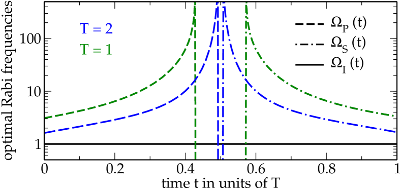
Figure 4: (Color online) Optimal half Rabi frequencies $\Omega_{P}(t)$, $\Omega_{I}(t)$, and $\Omega_{S}(t)$ (Case 2) for finite control times $T$ with relaxation rate $k=1$ and the amplitude bound on $\Omega_{I}$ set to one, $A=1$. For very short $T$ (Case 1), the optimal Rabi frequencies $\Omega_{S}(t)$ and $\Omega_{P}(t)$ correspond to instantaneous pulses of infinite power at $t=0$ and $t=T$; for $T\to\infty$, the hold period with zero $\Omega_{S}(t)$, $\Omega_{P}(t)$ in the middle of the time interval disappears.

For $0\leq t\leq\tau$, where $\tau$ is a function of $T$, $u_{2}^{*}(t)=1$ and $u_{1}^{*}(t)$ is increased gradually from a value $u_{1}^{*}(0)<1$ to $u_{1}^{*}(\tau)=1$. This corresponds to $\Omega_{p}(t)$ rising from its initial value $\Omega_{p}(0)$ to infinity while $\Omega_{s}(t)$ remains zero throughout the first phase, cf. Fig. 4. In the second phase, for time $\tau\leq t\leq T-\tau$, the optimal controls are $u_{1}^{*}(t)=u_{2}^{*}(t)=1$. This corresponds to both $\Omega_{p}(t)$ and $\Omega_{s}(t)$ being zero. Finally, for $t\geq T-\tau$, $u_{1}^{*}(t)=1$ and $u_{2}^{*}(t)$ is decreased from $u_{2}^{*}(T-\tau)=1$ to $u_{2}^{*}(T)=u_{1}(0)$. $\Omega_{s}(t)$ is thus decreased from infinity to its final value $\Omega_{s}(T)$ which is equal to $\Omega_{p}(0)$, while $\Omega_{p}(t)$ remains zero. The parameter $\tau$ determining the switching times is calculated from the following equation,

$$T=2\tau+{{\gamma_{2}-\gamma_{1}}\over{A}}\,,$$ (17)

where

$$\gamma_{1}=\cot^{-1}\left(\frac{1-\kappa(\tau)}{2\xi\kappa(\tau)}\right)\,,\ \ \gamma_{2}=\tan^{-1}\left(\frac{1-\kappa(\tau)}{2\xi}\right)\,,$$

and

$$\kappa(\tau) = 1+2\xi^{2}-$$

$$2\xi\sqrt{1+\xi^{2}}\coth\left(A\sqrt{1+\xi^{2}}\ \tau+2\sinh^{-1}\xi\right)\,.$$

In the limit of infinite time, $\tau=\frac{T}{2}$; in this case the ’hold’ phase in the middle, where only $\Omega_{I}(t)$ is non-zero, disappears (cf. the blue and green curves in Fig. 4). The optimal solution thus corresponds to the intuitive pulse sequence of pump first, then Stokes, not a STIRAP-like solution characterized by a counter-intuitive pulse sequence.

The efficiency of the population transfer, $\eta_{T}$, in case 2 is expressed for finite time $T$ in terms of the angles as

$$\eta_{T}=\frac{\exp(\xi(\gamma_{1}-\gamma_{2}))(1-\xi\sin 2\theta_{2})}{\sin(\gamma_{1}+\gamma_{2})}\,.$$ (18)

In the limit that $T$ goes to infinity, $\gamma_{1}=\gamma_{2}=\tan^{-1}\left(\sqrt{1+\xi^{2}}-\xi\right)$, and $\eta_{T}$ approaches $\eta$, the maximum transfer efficiency given by

$$\eta=\sqrt{1+\xi^{2}}-\xi\,.$$ (19)

We see that the transfer efficiency can reach unity only for $\xi=0$, i.e., $\frac{k}{A}=0$. This is the case of infinite power, i.e., the decay is much smaller than the maximum Rabi frequency coupling the intermediate states. When only limited power is available, the transfer efficiency is always less than unity.

Even for the case of a multiphoton resonance, no analytical optimal solutions are known for non-zero detunings. As shown in Refs. Vitanov et al. (1998); Nakajima (1999), adiabatically eliminating one of the two decaying intermediate levels allows one to recover a three-level system and thus the STIRAP solution. However, perfect adiabatic elimination in the presence of decay requires infinite power of the field coupling the intermediate levels. We believe that our conclusion for a finite power transfer efficiency of less than unity holds also for non-zero detunings.

To support this claim, consider the four-level system with non-zero detunings $\Delta_{2}$, $\Delta_{3}$,

$$\frac{d}{dt}\left(\begin{array}[]{c}x_{1}\\ x_{2}\\ x_{3}\\ x_{4}\end{array}\right)=-i\left(\begin{array}[]{cccc}0&\Omega_{p}&0&0\\ \Omega_{p}&\Delta_{2}-ik&\Omega_{i}&0\\ 0&\Omega_{i}&\Delta_{3}-ik&\Omega_{s}\\ 0&0&\Omega_{s}&0\end{array}\right)\left(\begin{array}[]{c}x_{1}\\ x_{2}\\ x_{3}\\ x_{4}\end{array}\right)\,.$$ (20)

Assume complete population transfer is possible in this system. Clearly, for this to hold the population of the intermediate states must remain zero during the process. If this is the case, the values of the detunings would not affect the transfer and we can therefore replace the detunings by zero. However, in this case the system reduces to Eq. (20), which we showed to be uncontrollable with finite power, leading to a contradiction with our assumption of controllability. Thus we claim that even with non-zero detunings, complete population transfer is not possible with finite pulse power if there are multiple decaying intermediate states. Since detuning relative to the intermediate states is known not to affect STIRAP efficiency Bergmann et al. (1998), this result is fully consistent with our prior expectations.

IV Generalization to $N$-level systems

In the previous section we showed that with two consecutive intermediate decaying states, the transfer efficiency with finite power is always less than one. If more than two intermediate decaying states are present, the transfer efficiency gets even worse. For example, suppose we have a chain of five states with three intermediate decaying states,

$$\frac{d}{dt}\left(\begin{array}[]{c}x^{\prime}_{1}\\ x^{\prime}_{2}\\ x^{\prime}_{3}\\ x^{\prime}_{4}\\ x^{\prime}_{5}\end{array}\right)=-i\left(\begin{array}[]{ccccc}0&\Omega_{p}&0&0&0\\ \Omega_{p}&-ik&\Omega_{1}&0&0\\ 0&\Omega_{1}&-ik&\Omega_{2}&0\\ 0&0&\Omega_{2}&-ik&\Omega_{s}\\ 0&0&0&\Omega_{s}&0\end{array}\right)\left(\begin{array}[]{c}x^{\prime}_{1}\\ x^{\prime}_{2}\\ x^{\prime}_{3}\\ x^{\prime}_{4}\\ x^{\prime}_{5}\end{array}\right)\,.$$

With a change of variables, letting $x_{1}=x_{1}^{\prime}$, $x_{2}=ix^{\prime}_{2}$, $x_{3}=-x_{3}^{\prime}$, $x_{4}=-ix_{4}^{\prime}$ and $x_{5}=x^{\prime}_{5}$, the dynamics become

$$\frac{d}{dt}\left(\begin{array}[]{c}x_{1}\\ x_{2}\\ x_{3}\\ x_{4}\\ x_{5}\end{array}\right)=\left(\begin{array}[]{ccccc}0&-\Omega_{p}&0&0&0\\ \Omega_{p}&-k&-\Omega_{1}&0&0\\ 0&\Omega_{1}&-k&-\Omega_{2}&0\\ 0&0&\Omega_{2}&-k&-\Omega_{s}\\ 0&0&0&\Omega_{s}&0\end{array}\right)\left(\begin{array}[]{c}x_{1}\\ x_{2}\\ x_{3}\\ x_{4}\\ x_{5}\end{array}\right)\,.$$

Introducing new variables $y_{i}$, the fifth state and fourth state can be combined,

$$y_{1}=x_{1}\,,\,y_{2}=x_{2}\,,\,y_{3}=x_{3}\,,\,y_{4}=\sqrt{x_{4}^{2}+x_{5}^{2}}\,.$$

This reduces the system to an effective four-state system,

$$\frac{d}{dt}\left(\begin{array}[]{c}y_{1}\\ y_{2}\\ y_{3}\\ y_{4}\end{array}\right)=\left(\begin{array}[]{cccc}0&-\Omega_{p}&0&0\\ \Omega_{p}&-k&-\Omega_{1}&0\\ 0&\Omega_{1}&-k&-\Omega_{2}\cos\theta\\ 0&0&\Omega_{2}\cos\theta&-k\cos^{2}\theta\end{array}\right)\left(\begin{array}[]{c}y_{1}\\ y_{2}\\ y_{3}\\ y_{4}\end{array}\right)\,,$$ (21)

where $\tan\theta=\frac{x_{5}}{x_{4}}$. The transfer efficiency for the dynamics of $y_{1},\ldots,y_{4}$, represents an upper bound to the transfer efficiency for the dynamics of $x_{1},\ldots,x_{5}$, since $y_{4}\geq x_{5}$: If a control scheme transfers an amount of population, $\eta$, from $x_{1}$ to $x_{5}$ then this scheme also transfers at least an amount of population $\eta$ from $y_{1}$ to $y_{4}$. Next we show that the efficiency of transfer from $y_{1}$ to $y_{4}$ according to the dynamics of Eq. (21) is upper bounded by the transfer efficiency for the dynamics of Eq. (13) of the four-level chain. To make the comparison transparent, we consider the following dynamics,

$$\frac{d}{dt}\left(\begin{array}[]{c}y^{\prime}_{1}\\ y^{\prime}_{2}\\ y^{\prime}_{3}\\ y^{\prime}_{4}\end{array}\right)=\left(\begin{array}[]{cccc}0&-\Omega_{p}&0&0\\ \Omega_{p}&-k&-\Omega_{1}&0\\ 0&\Omega_{1}&-k&-\Omega_{2}\cos\theta\\ 0&0&\Omega_{2}\cos\theta&0\end{array}\right)\left(\begin{array}[]{c}y^{\prime}_{1}\\ y^{\prime}_{2}\\ y^{\prime}_{3}\\ y^{\prime}_{4}\end{array}\right)\,.$$ (22)

Clearly the efficiency of transfer from $y_{1}$ to $y_{4}$ is upper bounded by the efficiency of transfer from $y^{\prime}_{1}$ to $y^{\prime}_{4}$ since the only difference between these two dynamics is that $y_{4}$ is subject to decay while $y^{\prime}_{4}$ is not. The efficiency of transfer from $y^{\prime}_{1}$ to $y^{\prime}_{4}$ in turn is upper bounded by the transfer efficiency for the four-level chain, Eq. (13), since the controls in Eq. (22) are more restricted than the controls in Eq. (13). This can be seen as follows: If a control scheme for the dynamics, Eq. (22), reaches an efficiency $\eta$, then simply setting $\Omega_{s}=\Omega_{2}\cos\theta$ in Eq. (13), the same transfer efficiency $\eta$ is obtained for the four-level chain. The inverse step of setting $\Omega_{2}=\frac{\Omega_{s}}{\cos\theta}$ is, however, not always possible, since this may lead to infinite $\Omega_{2}$.

From this line of argument, we see that the transfer efficiency of the five-state chain with three intermediate decaying states is upper bounded by the transfer efficiency of the four-state chain with two intermediate decaying states. Analogously, we can show that the transfer efficiency of the $N$-state chain $(N\geq 4)$ with $N-2$ intermediate decaying states is upper bounded by the transfer efficiency of the $N$-state chain with $N-3$ intermediate decaying states. That is for chains where all intermediate states are subject to decay, the transfer efficiency is monotonically decreasing with increasing length of the chain. In particular, we have the interesting result that for any chain with two or more consecutive intermediate decaying states, the efficiency will be less than unity.

Our analytical results allow us to draw a general inference about previous work on population transfer in $N$-level systems. Extensions of STIRAP from the three-level system to multi-level chains have been investigated since the early days of STIRAP (see Ref. Bergmann et al. (1998) and references therein). Although these mechanisms are designed to keep the population in the intermediate levels as small as possible, close inspection reveals that none of these succeed in completely avoiding intermediate population for finite power pulses, even for $T\to\infty$. In particular, we note that none of these schemes can keep the population for two consecutive intermediate states at zero. We illustrate this with three of the generalized STIRAP schemes. In Ref. Shore et al. (1991), a generalization of STIRAP for $N$-level chains was proposed for $N$ odd. In this scheme, the population in all the intermediate even levels can be kept at zero but placing population in the intermediate odd levels cannot be avoided. Clearly it is impossible to keep two neighbouring states empty. In Ref. Malinovsky and Tannor (1997), a STIRAP-like solution for $N$-level chains was found numerically, and termed straddling STIRAP. It consists in choosing the Rabi frequencies coupling the intermediate states to be at least one order of magnitude larger than $\Omega_{s}$ and $\Omega_{p}$ and overlapping in time with both $\Omega_{s}$ and $\Omega_{p}$. Inspection of the solution reveals that all intermediate levels acquire some population, and therefore it is impossible to keep two consecutive levels empty without using infinite power. The straddling STIRAP was analyzed further both analytically and numerically Vitanov et al. (1998); Nakajima (1999). It was clarified that for $N$ even, a non-zero detuning of the lasers coupling the intermediate states is required to obtain a STIRAP-like solution while for zero detunings, an intuitive (Rabi) pulse sequence is found. Moreover, it was shown that in the dressed state picture, a very strong coupling between the intermediate states moves the intermediate states out of resonance such that they are decoupled and effectively a two-level system ($N$ even with zero detuning) or a three-level system ($N$ odd or $N$ even with non-zero detuning) are recovered. It can be seen that whether $N$ is odd or even, avoiding population in two consecutive levels requires infinite power. Taking dissipation explicitly into account, it is clear that if two consecutive intermediate levels are subject to decay, unit transfer efficiency is impossible at finite power. Our analytical results including dissipation are consistent with this analysis.

V Controllability in the relaxation-free subspace

In this section, we will generalize the results of the previous sections to state-to-state controllability on relaxation-free subspaces $S$. Based on the results of the previous sections, we will characterize the relaxation-free subspaces that are finite-power controllable on the pure state space. Our argument is based on the assumption of selective control, i.e. the assumption that $\Omega_{s}$, $\Omega_{p}$ and any other coupling, can be tuned independently. This corresponds to the bare, field-free Hamiltonian having no degenerate levels or frequencies. With selective control, controllability on the relaxation-free subspace becomes equivalent to connectivity Polack et al. (2009).

Our central result is that a relaxation-free subspace is controllable on the pure state space if and only if any two eigenstates in the subspace can be connected by a path that never visits two consecutive states that both suffer relaxation. This is illustrated in Fig. 5

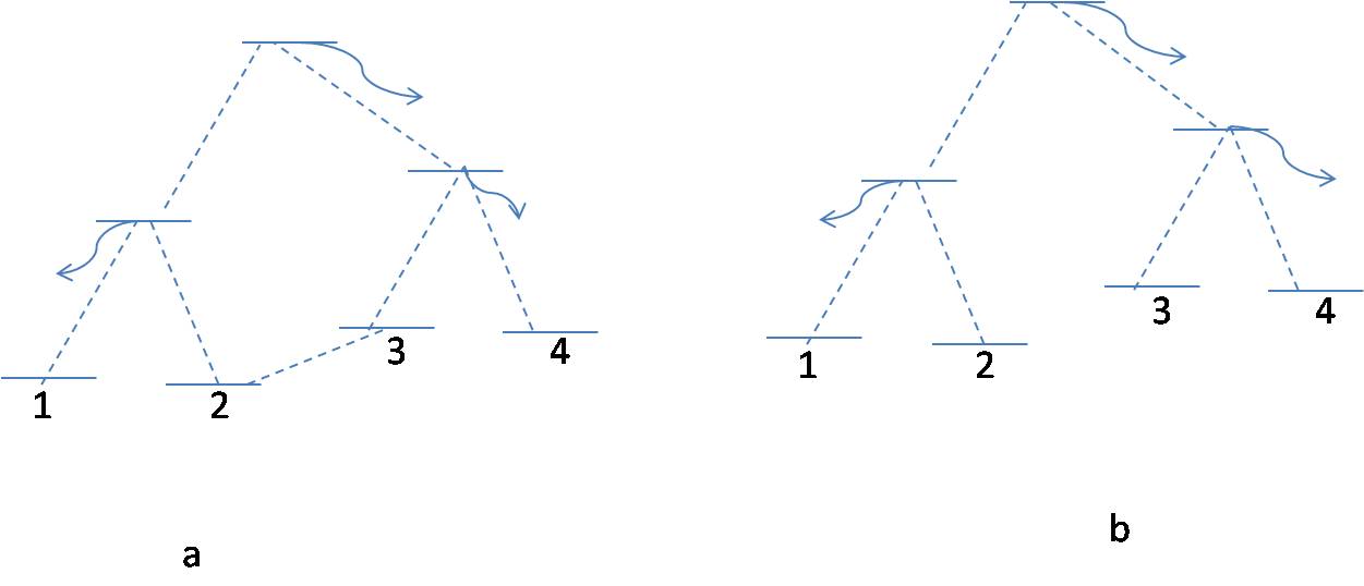
Figure 5: (Color online) Examples for (a) a system that is controllable in the subspace $\{|1\rangle,|2\rangle,|3\rangle,|4\rangle\}$ since any pair of eigenstates can be connected by a path that never visits two consecutive states that suffer relaxation; (b) a system that is not controllable in the subspace $\{|1\rangle,|2\rangle,|3\rangle,|4\rangle\}$ since one has to pass through three consecutive states that suffer relaxation to connect the states $|1\rangle$ and $|4\rangle$.

with part (a) displaying an example where any pair of eigenstates in the relaxation-free subspace $S=\{|1\rangle,|2\rangle,|3\rangle,|4\rangle\}$ can be connected by a path that never visits two consecutive states suffering relaxation, i.e. this system is state-to-state controllable in the space $S=\{|1\rangle,|2\rangle,|3\rangle,|4\rangle\}$. The system shown in Fig. 5(b) is not controllable in the relaxation-free subspace $S=\{|1\rangle,|2\rangle,|3\rangle,|4\rangle\}$ since one has to pass through three consecutive states that suffer relaxation in order to connect the states $|1\rangle$ and $|4\rangle$.

Clearly the condition is necessary. As from the previous section, we know that if any path has two intermediate states outside of the relaxation-free space, complete population transfer is not possible. Hence the system is not controllable. The condition is also sufficient. If there are never two states in a row that suffer relaxation, the control found in Section II allows us to traverse one intermediate relaxing state without losses. Concatenating such processes gives the result.

We can connect the controllability condition with the coupling topology of the system: The condition is fulfilled if and only if the eigenstates in the relaxation-free subspace are (I) directly connected via paths in the subspace; (II) connected by one intermediate state which suffers relaxation; (III) connected by concatenations of paths of type I and type II as sketched in Fig. 6.

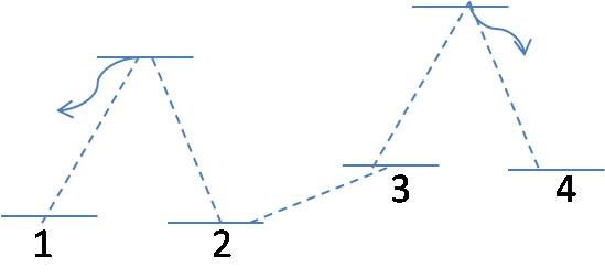
Figure 6: (Color online) The eigenstates $|1\rangle$ and $|4\rangle$ are connected by concatenating paths of type (I) and type (II).

Note that this coupling topology includes degenerate levels in the relaxation-free and the relaxing subspaces provided that a generalized Morris-Shore transformation can be employed to replace the coupled multi-level system by a set of two- and three-level systems and dark states (single levels) Rangelov et al. (2006).

We first show that with this coupling topology we can achieve coherent population transfer between any two eigenstates. Controllability is then achieved by applying sequences of these operations. First, if two eigenstates are connected via (I) we can obviously achieve coherent population transfer between them. It remains to be shown that coherent transformation is possible for two eigenstates that are connected by one intermediate state suffering relaxation. This is achieved by combining our results of Section II with the fractional STIRAP developed by Vitanov et al. Vitanov et al. (1999) to generate arbitrary coherent superpositions of $|1\rangle$ and $|3\rangle$ from the initial state $|1\rangle$. For two eigenstates $|1\rangle$ and $|3\rangle$ that are connected by an intermediate state $|2\rangle$ suffering relaxation, a coherent transformation from state $|1\rangle$ to $\cos\beta|1\rangle-e^{i\phi}\sin\beta|3\rangle$ is implemented by (i) adding a phase $\phi$ to the Stokes pulse such that the equations of motion read

$$\frac{d}{dt}\left(\begin{array}[]{c}x^{\prime}_{1}\\ x^{\prime}_{2}\\ x^{\prime}_{3}\end{array}\right)=-i\left(\begin{array}[]{ccc}0&\Omega_{p}&0\\ \Omega_{p}&-ik&\Omega_{s}e^{-i\phi}\\ 0&\Omega_{s}e^{i\phi}&0\end{array}\right)\left(\begin{array}[]{c}x^{\prime}_{1}\\ x^{\prime}_{2}\\ x^{\prime}_{3}\end{array}\right)\,,$$ (23)

and (ii) varying $\frac{\Omega_{p}}{\Omega_{s}}$ adiabatically from $0$ to $\tan\beta$. A general coherent transformation can be implemented by first applying the time-reversed version of this procedure in order to transfer the initial state to $|1\rangle$ and then to transfer $|1\rangle$ to the desired final state with the control scheme of Section II. We have thus shown controllability for eigenstates connected by (II). Obviously the results for (I) and (II) can be combined which yields controllability for (III) completing the proof of sufficiency.

So far we have considered only zero detunings. However, the result of controllability on the relaxation-free subspace also holds for non-zero detunings that can be represented by complex values for the decays. To see this, consider first a three-level system. It is well-known that the values of the detuning and the relaxation rate of the intermediate state do not affect the STIRAP efficiency Bergmann et al. (1998). This argument carries over to general N-level systems with non-zero detunings of the decaying states. If the system is controllable it can be viewed as a concatenation of two or more three-level STIRAP systems (and possibly type (I) paths), and then the detuning is irrelevant. If the system is uncontrollable, the detuning cannot make it controllable, based on the argument presented at the end of Section III.

VI Discussion and conclusions

We have considered the optimal control problem of transferring population in a quantum system between states in a subspace free of dissipation, where the transfer has to proceed via states that are subject to decay. We treated only the case of resonant controls with fixed carrier frequency and phases, controlling only the amplitudes of our pulses as a function of time. Such situations occur frequently in atomic and molecular physics applications. For example, transfer between different levels in the electronic ground manifold can proceed via Raman transitions. In quantum information applications, stable qubit states are often connected via auxiliary states that are subject to decay. In particular, this may be the case for logical qubits encoded in a decoherence-free subspace.

We have obtained analytical solutions to this optimal control problem by solving the Hamilton-Jacobi-Bellman equation for the optimal return function. For a single intermediate decaying state, we have recovered the Stimulated Raman Adiabatic Passage process Bergmann et al. (1998) as the globally optimal solution in the limit of infinite time. Perfect state transfer is achieved only in this limit. This is in accordance with experimental realizations where at best 99.5% state transfer were achieved Bergmann .

In Ref. Boscain et al. (2002), the STIRAP solution in a three-level system was previously obtained using geometric control methods. There, the optimal return function was specifically designed to avoid the hard pulses obtained by us (which cause the sudden population transfer from level 1 to 2 at $t=0$). Note that generalizing the results of Ref. Boscain et al. (2002) from the three-level system to $N$-level systems is hampered by the system’s state being represented in terms of six real variables, compared to two variables, $r_{1}$ and $r_{2}$, in our case.

In contrast to the analytical solutions presented here and in Ref. Boscain et al. (2002), Refs. Band and Magnes (1994); Wang and Rabitz (1996); Solá et al. (1999); Kis and Stenholm (2002) employ numerical optimization procedures based on the calculus of variations. Our current work may help to clarify the disagreement in the literature on whether STIRAP is obtained as a solution to an optimal control problem Band and Magnes (1994); Malinovsky and Tannor (1997); Solá et al. (1999): the assertion of Ref. Band and Magnes (1994) that adiabatic passage population transfer cannot be obtained as the solution to an optimal control problem implicitly assumes finite pulse fluence and finite control time. Yet adiabaticity, strictly speaking, does not comply with these assumptions.

We have also presented analytical solutions for the case of population transfer that proceeds via two consecutive intermediate decaying states. In particular, we have shown that the optimal control does not yield perfect state transfer even in the limit of infinite time, unless the pulse coupling the intermediate levels has infinite power. This gives an analytical framework for understanding an earlier control solution termed straddling STIRAP that was obtained numerically Malinovsky and Tannor (1997) and that is essentially based on adiabatically eliminating the intermediate levels Vitanov et al. (1998); Nakajima (1999). Taking dissipation explicitly into account, we have clarified that the adiabatic elimination of the decaying levels is possible only in the limit of infinite power.

Finally, we have generalized these results to characterize the topologies of paths that can be achieved in $N$-level systems by finite-power controls and in the presence of dissipation. Population transfer with unit efficiency is only possible if each decaying state is connected to two non-decaying states. Complete population transfer is then achieved in the adiabatic limit, i.e., in a sequence of STIRAP processes. Finite-power state-to-state controllability on the relaxation-free subspace is thus equivalent to connectivity Polack et al. (2009), augmented by the condition that only one out of two consecutive levels may be subject to dissipation.

Appendix A Optimal control for the three-level system

In this Appendix, we derive the solution of the optimal control problem for the three level system. As introduced in Section II, we are going to solve the Hamilton Jacobi Bellman equation, Eq. (5) with the classical Hamiltonian of the control problem defined in Eq. (6). Introducing adjoint variables $\lambda_{1}$, $\lambda_{2}$,

$$\lambda_{1}=\frac{\partial V}{\partial r_{1}}\,,\,\lambda_{2}=\frac{\partial V}{\partial r_{2}}\,,$$ (24)

where $V$ denotes the optimal return function, the Hamiltonian of the optimal control problem can be expressed as

$$\begin{aligned} H(u)&=-k\lambda_{1}r_{1}u^{2}-A\lambda_{1}r_{2}u+A\lambda_{2}r_{1}u=-k\lambda_{1}r_{1}\left[u^{2}+\frac{A}{k}\left(\frac{r_{2}}{r_{1}}-\frac{\lambda_{2}}{\lambda_{1}}\right)u\right]\\ &=-k\lambda_{1}r_{1}\left\{\left[u-\frac{A}{2k}\left(\frac{\lambda_{2}}{\lambda_{1}}-\frac{r_{2}}{r_{1}}\right)\right]^{2}-\left[\frac{A}{2k}\left(\frac{\lambda_{2}}{\lambda_{1}}-\frac{r_{2}}{r_{1}}\right)\right]^{2}\right\}\,.\end{aligned}$$ (25)

We rewrite the ratios appearing in Eq. (25) in terms of variables $a$ and $b$,

$$a=\frac{\lambda_{2}}{\lambda_{1}}\,,\,b=\frac{r_{2}}{r_{1}}\,.$$ (26)

The optimal return function is a non-decreasing function of $r_{1}$, $r_{2}$ [starting from a larger $r_{1}(0)$ or $r_{2}(0)$, one can achieve a larger $r_{2}(T)$]. Due to Eq. (24) we therefore find $\lambda_{1}\geq 0$, $\lambda_{2}\geq 0$ and hence $a\geq 0$. Since $\lambda_{1}\geq 0$ and $r_{1}\geq 0$, maximizing $H$ with respect to $u$ is equivalent to minimizing the function

$$f(u)=\left[u-\frac{A}{2k}(a-b)\right]^{2}\,.$$

If $a-b<0$, then the solution is the trivial one, $u^{*}=0$. We therefore conclude that obtaining a non-zero control requires $a-b\geq 0$. Later we will show explicitly that $a-b$ is a non-decreasing function of time. Since $b(0)=0$ and $a(0)\geq 0$, we have $a(t)-b(t)\geq 0$ for all times $t$. We further distinguish two cases.

Case I: If $\frac{A}{2k}(a-b)\geq 1$, then the minimum of $f(u)$ is achieved at the maximum value that $u=\cos\theta$ can take, $u^{*}=1$.

Case II: If $0\leq\frac{A}{2k}(a-b)<1$, then the minimum of $f(u)$ is achieved at $u^{*}=\frac{A}{2k}(a-b)$.

It is a standard result that, along the optimal trajectory $(r_{1}(t),r_{2}(t))$, the adjoint variables $(\lambda_{1}(t),\lambda_{2}(t))$ satisfy the equations

$$\frac{d\lambda_{1}}{dt} = -\frac{\partial H}{\partial r_{1}}\,,$$

$$\frac{d\lambda_{2}}{dt} = -\frac{\partial H}{\partial r_{2}}\,,$$

i.e.,

$$\frac{d}{dt}\left(\begin{array}[]{c}\lambda_{1}\\ \lambda_{2}\\ \end{array}\right)=\left(\begin{array}[]{cc}ku^{2}&-Au\\ Au&0\\ \end{array}\right)\left(\begin{array}[]{c}\lambda_{1}\\ \lambda_{2}\\ \end{array}\right)$$ (27)

with the terminal condition $\lambda_{1}(T)=0$, $\lambda_{2}(T)=1$.

With Eqs. (27) and (4), we can derive the dynamics for $a$ and $b$ along the optimal trajectory,

$$\frac{d}{dt}a =Aua^{2}-ku^{2}a+Au\,,$$ (28a)

$$\frac{d}{dt}b =Aub^{2}+ku^{2}b+Au\,.$$ (28b)

Therefore

$$\frac{d}{dt}(a-b)=(a+b)u[A(a-b)-ku]\,.$$ (29)

For the optimal trajectory starting at $(r_{1},r_{2})=(1,0)$, $b(0)=0$. Depending on $a(0)$ we have the following cases.

Case A: If $a(0)\geq\frac{2k}{A}$, we start in Case I, $u^{*}=1$. From equation (29), it follows that

$$\frac{d}{dt}(a-b)=(a+b)[A(a-b)-k]\geq k(a+b)\geq 0\,,$$

i.e., $a-b$ is non-decreasing. Therefore we will remain in Case I for the whole time interval. Substituting $u^{*}=1$ into the dynamical equation for $(\lambda_{1},\lambda_{2})$, Eq. (27), and running it backwards, we obtain

$$\frac{d}{dt}\left(\begin{array}[]{c}\lambda_{1}(T-t)\\ \lambda_{2}(T-t)\\ \end{array}\right)=\left(\begin{array}[]{cc}-k&A\\ -A&0\\ \end{array}\right)\left(\begin{array}[]{c}\lambda_{1}(T-t)\\ \lambda_{2}(T-t)\\ \end{array}\right)$$ (30)

with the initial condition $\lambda_{1}(T)=0$, $\lambda_{2}(T)=1$. Integrating this equation yields

$$\left(\begin{array}[]{c}\lambda_{1}(t)\\ \lambda_{2}(t)\end{array}\right)=\left(\begin{array}[]{c}\frac{1}{\omega}\left[-Ae^{-\frac{1}{2}(k+\omega)(T-t)}+Ae^{-\frac{1}{2}(k-\omega)(T-t)}\right]\\ \frac{1}{2\omega}\left[-e^{-\frac{1}{2}(k+\omega)(T-t)}(k-\omega)+e^{-\frac{1}{2}(k-\omega)(T-t)}(k+\omega)\right]\end{array}\right)\,,$$ (31e)

where

$$\omega=\left\{\begin{array}[]{ll}\sqrt{k^{2}-4A^{2}}&\textrm{if $k^{2}>4A^{2}$}\\ i\sqrt{4A^{2}-k^{2}}&\textrm{if $k^{2}<4A^{2}$}\\ \end{array}\right.$$

and

$$\left(\begin{array}[]{c}\lambda_{1}(t)\\ \lambda_{2}(t)\end{array}\right)=\left(\begin{array}[]{c}Ae^{-A(T-t)}(T-t)\\ e^{-A(T-t)}[A(T-t)+1]\end{array}\right)$$ (31j)

for $k^{2}=4A^{2}$. Solving the equation $a(0)=\frac{\lambda_{2}(0)}{\lambda_{1}(0)}=\frac{2k}{A}$ for $T$, we obtain a critical time, $T_{M}$. When $T\leq T_{M}$, the optimal control is to set $u^{*}=1$ for the whole time $[0,T]$. An analytical expression can be derived for $T_{M}$. For example, when $k^{2}>4A^{2}$,

$$T_{M}=\frac{\log\left[\frac{-2A^{2}+5k^{2}+3k\sqrt{k^{2}-4A^{2}}}{2(A^{2}+2k^{2})}\right]}{\sqrt{k^{2}-4A^{2}}}\,.$$ (32)

The other cases can also be worked out. The critical time $T_{M}$ as a function of the decay rate $k$ and the amplitude bound $A$ is displayed in Fig. 7.

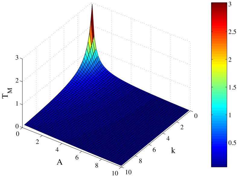
Figure 7: (Color online) The critical time $T_{M}$ as a function of decay rate $k$ and amplitude bound $A$. For control times $T$ shorter than $T_{M}$ the optimal control is simply set to $u^{*}=1$ for all $t\in[0,T]$, for control times larger than $T_{M}$, Eq. (7) applies.

$T_{M}$ takes large values corresponding to the trivial optimal solution $u^{*}=1$ for all $t\in[0,T]$ only for small decay rates and small amplitude bounds. As $k$ and $A$ increase, $T_{M}$ quickly becomes fairly small (for example, $T_{M}=0.06$ for $k=A=10$) and the optimal solution is determined according to Eq. (7).

Case B: If $a(0)<\frac{2k}{A}$, we start in Case II, $u^{*}=\frac{A}{2k}(a-b)$. From Eq. (29), we get in this case

$$\frac{d}{dt}(a-b) = (a+b)\frac{A}{2k}(a-b)\left[A(a-b)-\frac{A}{2}(a-b)\right]$$ (33)

$$= \frac{A^{2}}{4k}(a+b)(a-b)^{2}\geq 0$$

If $a(0)-b(0)=0$, then it will remain zero for the whole time. We will see that this only occurs as $T\rightarrow\infty$. If $a(0)>0$, then $a(t)-b(t)$ is strictly increasing, and at some time $\tau$, it will reach $\frac{2k}{A}$. We then switch to Case I, setting $u^{*}=1$ afterwards. So in this case, the optimal control is $u^{*}(t)=\frac{A}{2k}[a(t)-b(t)]$ for $t\leq\tau$ and $u^{*}(t)=1$ for $\tau<t\leq T$.

We now show how to calculate the switching time $\tau$ of Case B. Using Eqs. (28) and $u^{*}=\frac{A}{2k}(a-b)$, one can show that within the time interval $[0,\tau]$,

$$\frac{d}{dt}\left(\frac{a-b}{a+b}\right)=-\frac{A^{2}}{k}\left(\frac{a-b}{a+b}\right)^{2}\,.$$ (34)

Together with the initial condition, $\frac{a(0)-b(0)}{a(0)+b(0)}=1$, keeping in mind that $b(0)=0$, this yields

$$\frac{a(\tau)-b(\tau)}{a(\tau)+b(\tau)}=\frac{1}{\frac{A^{2}}{k}\tau+1}\,.$$ (35)

Since at time $t=\tau$, $a(\tau)-b(\tau)=\frac{2k}{A}$, we obtain

$$a(\tau) = A\tau+\frac{2k}{A}\,,$$ (36a)

$$b(\tau) = A\tau\,.$$ (36b)

In the time interval $[\tau,T]$, $u^{*}=1$, and we can again run Eq. (30) for $(\lambda_{1},\lambda_{2})$ backwards in time from $T$ to $\tau$. This yields another expression of $a(\tau)$ from Eqs. (31e) and (31j). Setting it equal to $A\tau+\frac{2k}{A}$, we obtain the switching time $\tau$.

Note that $T-\tau\leq T_{M}$. From Eqs. (36), the fact that $b(t)$ is non-negative for all times $t$ and $a(t)-b(t)$ is an increasing function, it follows that

$$a(t)>\frac{2k}{A}\quad\mathrm{for}\quad t\in[\tau,T]\,.$$

The assumption $T-\tau>T_{M}$ then leads to a contradiction: If $T-\tau>T_{M}$, then $a(T-T_{M})=2k/A$ at time $t=T-T_{M}$.

Next we evaluate the value of the optimal control $u^{*}(t)=\frac{A}{2k}[a(t)-b(t)]$ for $t\leq\tau$. We know that in the interval $[0,\tau]$, $a-b$ satisfies the dynamical equation, Eq. (33), which can be rewritten

$$\frac{d}{dt}(a-b)=\frac{A^{2}}{4k}\frac{a+b}{a-b}(a-b)^{3}\,.$$ (37)

From Eq. (35), we get $\frac{a+b}{a-b}=\frac{A^{2}}{k}t+1$. Substituting it into the above differential equation and solving it, we obtain $a(t)-b(t)$ for $t\in[0,\tau]$,

$$a(t)-b(t)=\frac{2k}{A}\frac{1}{\sqrt{A^{2}(\tau^{2}-t^{2})+2k(\tau-t)+1}}\,.$$ (38)

So in Case B, the optimal control is obtained to be

$$u^{*}(t)=\left\{\begin{array}[]{ll}\frac{1}{\sqrt{A^{2}(\tau^{2}-t^{2})+2k(\tau-t)+1}}&\textrm{for $t\in[0,\tau]$}\\ 1&\textrm{for $t\in[\tau,T]$}\\ \end{array}\right.\,.$$ (41)

In summary, there is a critical time, $T_{M}$, which depends on the relaxation rate $k$ and the amplitude bound $A$ and determines whether the control is switched or not: For $T\leq T_{M}$ the optimal control is just set to one, $u^{*}(t)=1$, for all times $t\in[0,T]$, and for $T>T_{M}$,

$$u^{*}(t)=\left\{\begin{array}[]{ll}\frac{1}{\sqrt{A^{2}(\tau^{2}-t^{2})+2k(\tau-t)+1}}&\textrm{for $t\in[0,\tau]$}\\ 1&\textrm{for $t\in[\tau,T]$}\\ \end{array}\right.\,.$$

The optimal control $u^{*}(t)$ is thus determined by the system parameters $A$ and $k$ and the switching time $\tau$ which is obtained by matching the dynamics of $a(t)$ at $t=\tau$, cf. Eqs. (36a) and (31).

We derive the optimal Rabi frequency, $\Omega_{p}(t)$, from $r_{1}(t)$, $r_{2}(t)$ and $u^{*}(t)$. From Eq. (2), it follows that

$$\frac{d}{dt}x_{2}=\Omega_{p}x_{1}-kx_{2}-\Omega_{s}x_{3}\,.$$ (42)

Substituting in Eq. (42) $x_{2}=r_{1}u$, $x_{1}=r_{1}\sqrt{1-u^{2}}$, and $x_{3}=r_{2}$, we obtain

$$\Omega_{p}=\frac{-ku^{2}r_{1}-Aur_{2}+r_{1}\dot{u}+kr_{1}u+Ar_{2}}{r_{1}\sqrt{1-u^{2}}}\,.$$ (43)

It is difficult to obtain a closed form of $\Omega_{p}(t)$, but Fig. 2 shows a few numerical examples. The solution $u^{*}(t)=1$ occurs toward the end of the interval $[0,T]$. For finite control times $T$, this solution for $u^{*}(t)$ corresponds to $\Omega_{p}(t)$ being infinity. For $T\to\infty$, a rescaling of time leads to finite $\Omega_{p}(t)$ as explained in Section II.2.

The interpretation of the optimal pulses is as follows: For small control time $T$, the major limitation for the population transfer is not due to relaxation, but the limited available time. The optimal choice $u^{*}=1$ maximizes the transfer speed, but also maximizes the decay of $r_{1}(t)$, respectively $x_{2}(t)$, as can be seen from Eq. (4). However, for a small available control time $T$, the gain obtained by maximizing the desired transfer at each moment is more important than the relaxation losses. As the control time $T$ increases, the relaxation degrades the performance more and more and the choice $u=1$ ceases to be optimal. For finite time the optimal solution becomes a compromise between maximizing the transfer speed and minimizing the decay. When time goes to infinity, minimizing the relaxation loss becomes more important than the transfer speed.

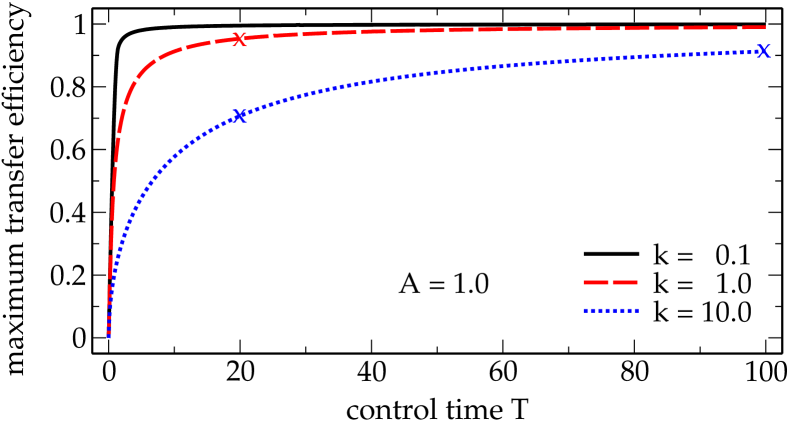
Figure 8: (Color online) The optimal transfer efficiency, $r_{2}(T)$ as a function of the control time $T$ for different relaxation rates $k$ (the maximum Rabi frequency, or pulse power, respectively, is limited by $A=1$). The curves are fairly concave, reaching a high transfer efficiency in relatively short time. This is compatible with the fact that in real experiments stimulated Raman adiabatic passage is actually done in relatively short time. To reach 100% transfer efficiency, however, infinite time is needed.

Substituting the optimal control $u^{*}(t)$ into the dynamics, Eq.(4), and integrating it yields the value of $r_{2}(T)$. For finite $T$ this gives an upper bound for the maximum achievable population transfer due to the possibility of $\Omega_{p}(t)$ going to infinity. As shown in Fig. 8 the upper bound approaches unity in the limit $T\to\infty$ even for large decay rates $k$, illustrating the recovery of STIRAP. For small and moderate decay rates, the convergence toward unit efficiency is much faster, reflecting the easier control problem.

References

- Bergmann et al. (1998) K. Bergmann, H. Theuer, and B. W. Shore, Rev. Mod. Phys. 70, 1003 (1998).
- Gaubatz et al. (1990) U. Gaubatz, P. Rudecki, S. Schiemann, and K. Bergmann, The Journal of Chemical Physics 92, 5363 (1990).
- Lang et al. (2008) F. Lang, K. Winkler, C. Strauss, R. Grimm, and J. H. Denschlag, Phys. Rev. Lett. 101, 133005 (2008).
- Ni et al. (2008) K.-K. Ni, S. Ospelkaus, M. H. G. de Miranda, A. Pe’er, B. Neyenhuis, J. J. Zirbel, S. Kotochigova, P. S. Julienne, D. S. Jin, and J. Ye, Science 322, 231 (2008).
- Shore et al. (1991) B. W. Shore, K. Bergmann, J. Oreg, and S. Rosenwaks, Phys. Rev. A 44, 7442 (1991).
- Malinovsky and Tannor (1997) V. S. Malinovsky and D. J. Tannor, Phys. Rev. A 56, 4929 (1997).
- Vitanov et al. (1998) N. V. Vitanov, B. W. Shore, and K. Bergmann, Eur. Phys. J. D 4, 15 (1998).
- Nakajima (1999) T. Nakajima, Phys. Rev. A 59, 559 (1999).
- Lidar and Whaley (2003) D. A. Lidar and K. B. Whaley, in Irreversible Quantum Dynamics, edited by F. Benatti and R. Floreani (Berlin, 2003), vol. 622 of Springer Lecture Notes in Physics, pp. 83–120.
- Monz et al. (2009) T. Monz, K. Kim, A. S. Villar, P. Schindler, M. Chwalla, M. Riebe, C. F. Roos, H. Häffner, W. Hänsel, M. Hennrich, et al., Phys. Rev. Lett. 103, 200503 (pages 4) (2009).
- Fortunato et al. (2002) E. M. Fortunato, L. Viola, J. Hodges, G. Teklemariam, and D. G. Cory, New J. Phys. 4, 5 (2002).
- Hornung et al. (2002) T. Hornung, S. Gordienko, R. de Vivie-Riedle, and B. J. Verhaar, Phys. Rev. A 66, 043607 (2002).
- Bertsekas (2005) D. P. Bertsekas, Dynamic Programming and Optimal Control (Athena Scientific, Belmont, Massachussetts, 2005), 3rd ed.
- Khaneja et al. (2003) N. Khaneja, T. Reiss, B. Luy, and S. J. Glaser, J. Magnet. Reson. 162, 311 (2003).
- Polack et al. (2009) T. Polack, H. Suchowski, and D. J. Tannor, Phys. Rev. A 79, 053403 (2009).
- Rangelov et al. (2006) A. A. Rangelov, N. V. Vitanov, and B. W. Shore, Phys. Rev. A 74, 053402 (2006).
- Vitanov et al. (1999) N. V. Vitanov, K.-A. Suominen, and B. W. Shore, J. Phys. B: At. Mol. Opt. Phys. 32, 4535 (1999).
- (18) K. Bergmann, private communication.
- Yatsenko et al. (1998) L.P. Yatsenko, B.W. Shore, K. Bergmann, and V.I. Romanenko, Eur. Phys. J. D 4, 47-56 (1998).
- Band and Magnes (1994) Y. B. Band and O. Magnes, J. Chem. Phys. 101, 7528 (1994).
- Wang and Rabitz (1996) N. Wang and H. Rabitz, J. Chem. Phys. 104, 1173 (1996).
- Solá et al. (1999) I. R. Solá, V. S. Malinovsky, and D. J. Tannor, Phys. Rev. A 60, 3081 (1999).
- Kis and Stenholm (2002) Z. Kis and S. Stenholm, J. Mod. Opt. 49, 111 (2002).
- Boscain et al. (2002) U. Boscain, G. Charlot, J.-P. Gauthier, S. Guérin, and H.-R. Jauslin, J. Math. Phys. 43, 2107 (2002).